Viability of Boosted Light Dark Matter in a Two-Component Scenario

Abstract

We study the two-component boosted dark matter (DM) scenario in a neutrinophilic two-Higgs doublet model ($\nu 2$HDM), which comprises of one extra Higgs doublet with a MeV scale CP-even scalar H. This model is extended with a light ($\sim 10$ MeV) singlet scalar DM $\phi_{3}$, which is stabilized under the existing $Z_{2}$ symmetry and can only effectively annihilate through scalar $H$. As the presence of a light H modify the oblique parameters to put tight constraints on the model, introduction of vectorlike leptons (VLL) can potentially salvage the issue. These additional vector-like doublet $N$ and one vector-like singlet $\chi$ are also stabilized through the $Z_{2}$ symmetry. The lightest vectorlike mass eigenstate $\chi_{1}$ ($\sim 100$ GeV) can be the potential second DM component of the model. Individual scalar and fermionic DM candidates have Higgs/Z mediated annihilation, restricting the fermion DM in a narrow mass region while a somewhat broader mass region is allowed for the scalar DM. In a coupled scenario, light DM $\phi_{3}$ gets its boost from the $\chi_{1}$ annihilation while the fermionic DM opens up new annihilation channel $\chi_{1}\chi_{1}\to\phi_{3}\phi_{3}$: decreases the relic density. This paves way for more fermionic DM mass with under-abundant relic, a region of [35-60] GeV compared to a smaller [40-50] GeV window for the single component fermion DM. On the other hand, the $\phi_{3}$ resonant annihilation gets diluted due to boosting effects in kinematics, which increases the DM relic leading to a smaller allowed region. To achieve an under-abundant relic, the total DM relic will be dominated by the $\chi_{1}$ contribution. While there is a region with $\phi_{3}$ contribution dominating the total DM, the combined relic becomes over-abundant. Therefore, a sub-dominant ($\sim 5\%$) boosted scalar is the most favorable light DM candidate to be probed for detection.

1 Introduction

One of the main ignition behind our quest for new physics is the existence of Dark Matter (DM) whose presence is already established in the experiments, but only through indirect gravitational probes, such as galaxy rotation curves, cosmic microwave background radiation and gravitational lensing Zwicky:1933gu ; Begeman:1991iy ; Bertone:2010zza ; Bauer:2017qwy ; Bertone:2004pz ; Lisanti:2016jxe among others. Precise measurements at these experiments predict the amount of DM in the present Universe to be around ($\sim 26.8\%$) of the total energy density of the Universe. In the conventional relic density terms, the DM abundance varies in the range $\Omega h^{2}\sim[0.11-0.13]$ at $3\sigma$ confidence level Planck:2015fie . The information from the structure formation in the early universe typically prefers the cold dark matter (CDM) scenario as it fits all the evidences. If we assume the CDM to be of a particle nature Bertone:2004pz , then the experiments are yet to ascertain the exact nature of the dark matter candidate/s. Similar to the visible sector, the dark sector may as well consist of multiple dark matter candidates Zurek:2008qg ; Bhattacharya:2019tqq . Dark matter candidates can be of different types as well – fermion, scalar or gauge boson.

Plethora of dark matter direct and indirect detection experiments are searching for dark matter signal. So far, these experiments are only successful to give us some hints and limits on the dark matter masses and interaction strengths DAMA:2008jlt ; XENON:2020rca ; XENON:2022ltv . Traditionally, weakly interacting massive particles (WIMPs) refId0 ; Arcadi:2017kky are proposed as dark matter candidates, with masses at the TeV scale, but none of them have been detected so far. Hence, the hunt for detecting dark matter in a territory below the GeV scale, which is hitherto not so explored has begun. In the Direct Detection experiments, the DM particles collide with the nuclei of target material and transfer a part of their kinetic energy to the target. In conventional DM direct detection method, the nuclear recoil energy is then measured by the detectors. When the dark matter is light, to be precise at the sub-GeV level, the roadblock to their detection comes from their inability to make the nuclei recoil. This is because the dark matter particles coming from the galaxies are non-relativistic, with velocity ($v\sim 10^{5}$ m/s). Hence the Kinetic energy of the recoiled particle is not sufficient to overcome the threshold $\sim\mathcal{O}$ (1 keV-1 MeV) in the direct detection experiments such as Xenon XENON:2020gfr etc.

A light dark matter can only make a massive nuclei recoil if it is boosted to relativistic velocities. Examples of boosted DM are Cosmic Rays Bringmann:2018cvk ; Das:2021lcr ; Xia:2022tid , Diffuse Supernova Neutrino Back- ground (DSNB) Arguelles:2017atb ; Das:2021lcr and blazers Bhowmick:2022zkj ; Wang:2021jic ; Granelli:2022ysi ; Maity:2022exk . In that case the light DM can deposit a recoil energy greater than the recoil threshold energy. This boost not only enhances it detectability in the DM direct detection experiments but also have intricate connections with the relic density related phenomenology also. The detection of lower DM masses is possible only if the scattering cross section is large because the flux of the boosted Dark matter is much smaller than the CDM population in the galaxies. There had been many studies to address the Boosted Dark Matter (BDM) in the literature (Ref 8-20 of Bardhan:2022bdg where boost is achieved via different mechanisms. One of the popular mechanism is when DM inside the galaxy collide with the high energy cosmic ray particles and gets a boost.

In this paper, we analyse an alternate mechanism following the footsteps of Agashe:2015xkj , where the heavier dark dark matter annihilates to light dark matter candidate and the mass difference between them plays the key role to produce the boost. We choose this framework of two-component dark matter scenario which is very interesting on its own merit Belanger:2011ww . There are papers in the literatures where particular models had been proposed to address the interaction of the boosted Dark matter via different models mostly in the framework of Self Interacting Dark Matter (SIDM) Dutta:2021wbn ; Borah:2021yek ; Baek:2021yos or others Ko:2022kvl . In such studies dark matter either interacts with the dark gauge boson or portal interactions are assumed. Most of the earlier works focus on different external mechanism to have a boosted DM and their possible detection intricacies. On the other hand, our work concentrate on a different side of the boosted DM sector, focusing on the relic density aspects of the combined two component DM paradigm, where one of the DM candidate is boosted from the annihilation of the other relatively heavier DM of the model.

We incorporate the boosted dark matter in a two component model framework, which can be embedded in a larger theory. Moreover, this framework not only addresses the relic abundance, but also satisfies other phenomenological constraints Grimus:2007if ; Grimus:2008nb ; Haber:2010bw from different experiments such as the LEP, LHC etc. In this paper, we have considered a neutrinophilic two Higgs doublet model ($\nu\rm 2HDM$) Machado:2015sha ; Nomura:2017jxb , where one CP even neutral scalar ($H$) can be very light in addition to a light right-handed (RH) neutrinos $N_{R_{i}}$. This model can successfully generate neutrino mass via Type II seesaw mechanism as well as the correct relic density, which has been discussed in Ref. Mohanty:2018iop . The $\nu\rm 2HDM$Ellis:2014dza is further extended with a scalar DM sector to incorporate one gauge singlet scalar $\phi_{3}$, which is the scalar dark matter candidate in our Model. We also extend the model with vectorlike fermions. Addition of the vectorlike fermions do allow for more favorable parameter space when precision observable constrains are considered in the extended $\nu 2HDM$ model. We choose one vector-like doublet ($N$) and one vector-like singlet ($\chi$) and we obtain the fermionic DM $\chi_{1}$ from the mixing of the former two vectorlike particles.

In this two component DM model, the boosting is achieved through the annihilation $\chi_{1}\chi_{1}\to\phi_{3}\phi_{3}$. This is the process that couples the vectorlike lepton and the scalar dark sector. The relic density of the dark matter is achieved by solving the Boltzmann Equations (BE) for two cases: I. When the scalar and vectorlike sectors are uncoupled, and II. when these two sectors are coupled. We study both the scenarios in detail and present a comparison of the individual and coupled scenario of the DM. In both the scenarios, we obtain the correct relic density for some selected benchmark points. We also show that scalar DM gets sufficient boost in the coupled scenario, leading to significant modification in its DM phenomenology. Moreover, unlike other scenarios studied in the literature, both the DM particles interact with the SM giving a very rich phenomenology. Overall, we present an well established Beyond Standard Model scenario to arrange a complete two component dark matter model, boosted DM being important feature of it.

2 Two Component Dark Matter Model

We consider the Two component Dark Matter scenario with the neutrinophilic Two-Higgs doublet model, in-short $\nu$2HDM, with an additional scalar singlet $\phi_{3}$, one vector-like doublet ($N$) and one vector-like singlet ($\chi$) Machado:2015sha ; Mohanty:2018iop ; Drees:2021rsg In this model, $\phi_{3}$ is the scalar Dark matter candidate and the combination of the Vectorlike particles gives the second component of the DM. Whereas, the neutral scalars of $\nu$2HDM provides the portal interaction between the two DM components. The $\nu$2HDM theory is based on the symmetry group $SU(3)_{c}\times SU(2)_{L}\times U(1)_{Y}\times Z_{2}$. The model contains electro-weak gauge singlet right-handed (RH) neutrinos, $N_{R_{i}}$ ($i$=1,2,3), for each flavor of Standard Model (SM) leptons and two Higgs doublets, $\Phi_{1}$ and $\Phi_{2}$. All the charged fermions of SM and the Higgs doublet $\Phi_{1}$, are even under the discrete symmetry, $Z_{2}$, while RH neutrinos and the Higgs doublet $\Phi_{2}$ are odd under $Z_{2}$. The complete particle/field content is listed in Table: 1

Particle Name	$SU(2)_{L}$ Charges	$U(1)_{Y}$ Charges	$Z_{2}$ Charges
Scalar Fields
$\Phi_{1}$	2	1	1
$\Phi_{2}$	2	1	-1
$\phi_{3}$	1	0	-1
Fermionic Fields
N	2	-1	-1
$\chi$	1	0	-1

Table 1: The BSM fields and their charge assignments.

The most general scalar potential for a CP-conserving 2HDM Branco:2011iw can be written as,

$$V = m_{11}^{2}\Phi_{1}^{{\dagger}}\Phi_{1}+m_{22}^{2}\Phi_{2}^{{\dagger}}\Phi_{2}-(m_{12}^{2}~{}\Phi_{1}^{{\dagger}}\Phi_{2}+h.c.)+\frac{\lambda_{1}}{2}(\Phi_{1}^{{\dagger}}\Phi_{1})^{2}+\frac{\lambda_{2}}{2}(\Phi_{2}^{{\dagger}}\Phi_{2})^{2}$$ (1)

$$+ \lambda_{3}(\Phi_{1}^{{\dagger}}\Phi_{1})(\Phi_{2}^{{\dagger}}\Phi_{2})+\lambda_{4}(\Phi_{1}^{{\dagger}}\Phi_{2})(\Phi_{2}^{{\dagger}}\Phi_{1})$$

$$+ \Bigg{[}\frac{\lambda_{5}}{2}(\Phi_{1}^{{\dagger}}\Phi_{2})^{2}+\lambda_{6}(\Phi_{1}^{\dagger}\Phi_{1})(\Phi_{1}^{\dagger}\Phi_{2})+\lambda_{7}(\Phi_{2}^{\dagger}\Phi_{2})(\Phi_{1}^{\dagger}\Phi_{2})+h.c.\Bigg{]}.$$

where $\Phi_{1}$ and $\Phi_{2}$ are two $SU(2)_{L}$ Higgs doublets. If we assume a $Z_{2}$ symmetry under which $\Phi_{1}$ is even and $\Phi_{2}$ is odd, then the coefficients $m_{12}$ = $\lambda_{6}$ = $\lambda_{7}$ = 0. However, one can allow a softly broken $Z_{2}$ symmetry assuming small non-zero values of $m_{12}$ while keeping $\lambda_{6}$ = $\lambda_{7}$ = 0.

The elements of the two Higgs doublets are in general complex and can be written (in unitary gauge) as,

$$\Phi_{1}=\frac{1}{\sqrt{2}}\left(\begin{array}[]{c}\sqrt{2}(v_{2}/v)H^{+}\\ h_{0}+v_{1}+i(v_{2}/v)A\\ \end{array}\right),$$ (4)

$$\Phi_{2}=\frac{1}{\sqrt{2}}\left(\begin{array}[]{c}-\sqrt{2}(v_{1}/v)H^{+}\\ H_{0}+v_{2}-i(v_{1}/v)A\\ \end{array}\right)$$ (7)

where $v_{1}$ and $v_{2}$ are the vacuum expectation values (vev) of the two Higgs doublets, namely $v_{1}=\langle\Phi_{1}\rangle$ and $v_{2}=\langle\Phi_{2}\rangle$ with $v^{2}=v^{2}_{1}+v^{2}_{2}$. After the electroweak symmetry breaking (EWSB), the two Higgs doublets mix with each other to produce two CP-even neutral Higgs bosons (h and H), one CP-odd neutral Higgs boson (A) and a pair of charged Higgs boson ($H^{\pm}$). Three massless Goldstone bosons are also generated which resulted into the longitudinal modes of the W and Z bosons.

The mass eigenstates h, and H are related to the weak eigenstates $h_{0}$, and $H_{0}$ by,

$$h_{0}=H\cos\alpha-h\sin\alpha,~{}H_{0}=H\sin\alpha+h\cos\alpha.$$ (8)

There is an orthogonal mixing between the charged and CP-odd Higgs states with corresponding charged and neutral Goldstone modes with a mixing angle $\beta$, where $\tan\beta=\frac{v_{2}}{v_{1}}$.

The masses of physical Higgs bosons (both charged and neutral) can be written as,

$$m_{h}^{2} = M^{2}c_{\beta-\alpha}^{2}+v^{2}\Big{[}\lambda_{1}s_{\alpha}^{2}c_{\beta}^{2}+\lambda_{2}c_{\alpha}^{2}s_{\beta}^{2}-\frac{1}{2}\lambda_{345}~{}\sin 2\alpha~{}\sin 2\beta\Big{]}$$ (9)

$$m_{H}^{2} = M^{2}s_{\beta-\alpha}^{2}+v^{2}\Big{[}\lambda_{1}c_{\alpha}^{2}c_{\beta}^{2}+\lambda_{2}s_{\alpha}^{2}s_{\beta}^{2}+\frac{1}{2}\lambda_{345}~{}\sin 2\alpha~{}\sin 2\beta\Big{]}$$ (10)

$$m_{A}^{2} = M^{2}-\lambda_{5}~{}v^{2}$$ (11)

$$m_{H^{\pm}}^{2} = M^{2}-\frac{\lambda_{45}}{2}~{}v^{2}$$ (12)

where $\lambda_{345}=\lambda_{3}+\lambda_{4}+\lambda_{5}$, $\lambda_{45}=\lambda_{4}+\lambda_{5}$, $M^{2}=\frac{m_{12}^{2}}{s_{\beta}~{}c_{\beta}}$, and

$$\tan 2\alpha=\frac{-m_{12}^{2}+\lambda_{345}~{}v^{2}\sin 2\beta}{-2m_{12}^{2}~{}\cot 2\beta+v^{2}(\lambda_{1}~{}c_{\beta}^{2}-\lambda_{2}~{}s_{\beta}^{2})+v^{2}~{}\lambda_{345}\cos 2\beta}.$$ (13)

One can always choose to work in the physical mass basis over the gauge basis, and assume the physical masses being the free parameters along with the Higgs mixing angle and $v_{2}$. In this basis, the quartic couplings can be expressed in terms of the physical masses, vevs, and mixing angles. We ensure that all the quartic couplings satisfy the limits coming from the stability of the vacuum and tree-level perturbative unitarity.

The triple Higgs coupling constants, in terms of the free parameters of the model, can be written as,

$$\lambda_{hHH} = \frac{1}{2}(\lambda_{3}+\lambda_{4}+\lambda_{5})\Big{[}v_{2}c_{\alpha}^{3}-v_{1}s_{\alpha}^{3}+2v_{1}s_{\alpha}c_{\alpha}^{2}-2v_{2}s_{\alpha}^{2}c_{\alpha}\Big{]}$$ (14)

$$+ \Big{[}3\lambda_{2}v_{2}c_{\alpha}s_{\alpha}^{2}-3\lambda_{1}v_{1}s_{\alpha}c_{\alpha}^{2}\Big{]}$$

$$\lambda_{hhH} = \frac{1}{2}(\lambda_{3}+\lambda_{4}+\lambda_{5})\Big{[}v_{2}s_{\alpha}^{3}+v_{1}c_{\alpha}^{3}-2v_{2}s_{\alpha}c_{\alpha}^{2}-2v_{1}s_{\alpha}^{2}c_{\alpha}\Big{]}$$ (15)

$$+ \Big{[}3\lambda_{1}v_{1}c_{\alpha}s_{\alpha}^{2}+3\lambda_{2}v_{2}s_{\alpha}c_{\alpha}^{2}\Big{]}$$

$$\lambda_{hhh} = (\lambda_{3}+\lambda_{4}+\lambda_{5})\Big{[}v_{2}c_{\alpha}s_{\alpha}^{2}-v_{1}s_{\alpha}c_{\alpha}^{2}\Big{]}+\Big{[}\lambda_{2}v_{2}c_{\alpha}^{3}-\lambda_{1}v_{1}s_{\alpha}^{3}\Big{]}$$ (16)

$$\lambda_{HHH} = (\lambda_{3}+\lambda_{4}+\lambda_{5})\Big{[}v_{2}c_{\alpha}^{2}s_{\alpha}+v_{1}s_{\alpha}^{2}c_{\alpha}\Big{]}+\Big{[}\lambda_{2}v_{2}s_{\alpha}^{3}+\lambda_{1}v_{1}c_{\alpha}^{3}\Big{]}$$ (17)

The Yukawa interaction in this model in the flavor basis takes the form,

$$\mathcal{L}_{Y}=Y^{d}_{\alpha\beta}\bar{Q}_{L,\alpha}\Phi_{1}d_{R,\beta}+Y^{u}_{\alpha\beta}\bar{Q}_{L,\alpha}\tilde{\Phi}_{1}u_{R,\beta}+Y^{l}_{\alpha\beta}\bar{L}_{L,\alpha}\Phi_{1}l_{R,\beta}+Y^{\nu}_{\alpha\beta}\bar{L}_{L,\alpha}\tilde{\Phi}_{2}N_{R,\beta}+\mathrm{h.c.}$$ (18)

where the doublets are $\bar{Q}_{L}^{T}=(u_{L}\ \ d_{L})$ and $\bar{L}_{L}^{T}=(\nu_{L}\ \ l_{L})$. The added three right handed neutrinos are gauge singlet Majorana neutrinos $N_{R,\beta}$, all of which transform as odd under the $Z_{2}$ symmetry, while all the SM fermions being $Z_{2}$ invariant.

If we restrict our model to only one right handed Majorana neutrino $N_{R}$, then the relevant Yukawa and mass terms of the right handed neutrino in the mass basis of the SM neutrinos are written as,

$$\mathcal{L_{N_{R}}}=y_{i}\bar{L}_{i}\tilde{\Phi}_{2}N_{R}+\frac{m_{N_{R}}}{2}N_{R}N_{R}.$$ (19)

Here the Yukawa couplings $y_{i}$ are mixture of flavor basis Yukawas $Y_{\alpha\beta}$ for one particular right handed Majorana neutrino. The neutrino mass matrix takes the form:

$$M_{\nu_{i}}=\begin{pmatrix}0\ \ \frac{y_{i}v_{2}}{\sqrt{2}}\\ \frac{y_{i}v_{2}}{\sqrt{2}}\ \ \frac{m_{N_{R}}}{2}\end{pmatrix}.$$ (20)

Diagonalizing this matrix we compute Majorana neutrino mass to be

$$m_{\nu_{i}}=\frac{y_{i}^{2}v_{2}^{2}}{m_{N_{R}}}.$$ (21)

This allows us to achieve a low scale seesaw mechanism, which was first proposed in the Ref. Ma:2000cc . With a Yukawa coupling $y_{i}\sim O(0.1)$, we get the Majorana neutrino mass of $0.1$ eV for $v_{2}\approx 10$ keV with right handed neutrino mass $m_{N_{R}}\sim 10$ MeV.

After the EW symmetry breaking, the couplings of the Higgs bosons h and H with the right-handed Neutrino are given by,

$$\lambda_{hN_{R}\nu_{L}}=-\frac{Y_{\nu}}{\sqrt{2}}s_{\beta}~{}~{};~{}~{}\lambda_{HN_{R}\nu_{L}}=\frac{Y_{\nu}}{\sqrt{2}}c_{\beta}.$$ (22)

We extend the model further to include a gauge singlet scalar $\phi_{3}$ which is odd under $Z_{2}$ symmetry. The scalar potential is now extended with the following additional term,

$$V_{DM}=\frac{1}{2}m_{\phi_{3}}^{2}\phi_{3}^{2}+\frac{\lambda_{\phi_{3}}}{4!}\phi_{3}^{4}+\kappa_{1}\Phi_{1}^{{\dagger}}\Phi_{1}\phi_{3}^{2}+\kappa_{2}\Phi_{2}^{{\dagger}}\Phi_{2}\phi_{3}^{2}.$$ (23)

The above potential includes four free parameters, namely $m_{\phi_{3}}$, $\lambda_{\phi_{3}}$, $\kappa_{1}$ and $\kappa_{2}$, among these $\lambda_{\phi_{3}}$ does not play any role for Higgs-portal interactions, so we set this to unity. The couplings between the DM particle ($\phi_{3}$) with the other neutral scalars play crucial role in the production of the light DM particle ($\phi_{3}$). In the alignment limit $c_{\beta-\alpha}=0$, these couplings can be expressed as:

$$\lambda_{\phi_{3}\phi_{3}h}=(\kappa_{1}c_{\beta}^{2}+\kappa_{2}s_{\beta}^{2})v$$ (24)

$$\lambda_{\phi_{3}\phi_{3}H}=\frac{1}{2}(\kappa_{1}-\kappa_{2})\sin 2\beta~{}v$$ (25)

$$\lambda_{\phi_{3}\phi_{3}hh}=\frac{1}{2}(\kappa_{1}c_{\beta}^{2}+\kappa_{2}s_{\beta}^{2})$$ (26)

$$\lambda_{\phi_{3}\phi_{3}HH}=\frac{1}{2}(\kappa_{1}s_{\beta}^{2}+\kappa_{2}c_{\beta}^{2})$$ (27)

$$\lambda_{\phi_{3}\phi_{3}hH}=\frac{1}{2}(\kappa_{1}-\kappa_{2})\sin 2\beta.$$ (28)

At this point, let us discuss the mass spectrum of the particles introduced till now. We choose the mass parameter $m_{\phi_{3}}$ in such a manner such that the mass of the scalar DM particle lies in the MeV scale (or at maximum up to a GeV), which in turn helps us to incorporate a light mediator particle in the model. The values of $\kappa_{1}$ and $\kappa_{2}$, which are essentially the Higgs-portal couplings, are kept small, namely we set them at 0.001 and 0.002 respectively. To achieve the small mediator mass, we set $v_{1}$ = 246 GeV and vary $v_{2}$ between 1 MeV to 1 GeV, such that the alignment limit is satisfied i.e., $\beta-\alpha\approx\frac{\pi}{2}$. This results in very small $\tan\beta\sim$ $\mathcal{O}(10^{-4})$, which in turn gives very small values of $\cos(\beta-\alpha)$. Hence, the neutral scalar $h$ effectively behaves like a SM Higgs boson at 125 GeV and a very light CP-even neutral Higgs boson ($H$) mediator with mass around 20 MeV is obtained.

Hence, we expect that the constraint on the various couplings of the SM Higgs boson are also satisfied by $h$. Furthermore, the existence of a light mediator particle ($H$) and light scalar DM candidate leads to additional contribution to the SM Higgs boson width through the invisible mode $h\to HH$ and $h\to\phi_{3}\phi_{3}$. We have checked that total rate at which the SM-like Higgs boson (h) decays invisibly is less that 10%, being consistent with the measurements CMS:2023sdw . In fact, using HiggsTools Bahl:2022igd , we check the choices of the masses and couplings used for the benchmark point for later sections are consistent with the measurements of the SM-like Higgs boson ($h$) at the LHC. Note that, due to the suppressed coupling with the $Z$ boson, no additional contributions are expected to come to the invisible width of the $Z$ boson, so the current bounds will be satisfied trivially CMS:2022ett .

The charged Higgs production at the LHC in the context of $\nu$2HDM is same as in 2HDM, however, due to the smallness of the mixing between the two Higgs bosons, the decays of charged Higgs to quarks are highly suppressed by the mixing factor $\tan\beta$. Charged scalars decaying through $H^{\pm}\rightarrow l^{\pm}\nu$ modes were already searched at the LEP and the mass the charged Higgs was constrained as $m_{H^{\pm}}$> 80 GeV ALEPH:2013htx . The smallness of $v_{2}$ and given the mass spectrum, the dominant decay mode of $H^{\pm}$ is $H^{\pm}\rightarrow W^{\pm}H$ with $H$ decaying to neutrinos. Evidently, search for charged Higgs boson through this mode will receive large irreducible SM backgrounds. Further, note that charged Higgs bosons can also contribute to the rate of the SM-like Higgs boson decay into diphoton through loops Seto:2015rma and the Pseudoscalar Higgs $A$ couples dominantly to neutrinos. In this work, we set the masses of the charged Higgs boson and the CP-odd neutral Higgs boson at 500 GeV. With these choices the above-mentioned bounds, including the constraints from flavor physics and astrophysical observations will be easily satisfied Bertuzzo:2015ada ; Sher:2011mx .

Due to the above-mentioned choice of the masses of the scalar particles, we expect that the oblique parameters ($S,T,U$) Peskin:1991sw will play a crucial role in constraining the parameter space Grimus:2007if ; Grimus:2008nb ; Haber:2010bw . In particular, the $S$ parameter is highly sensitive to the new physics effects at scales lower than $M_{Z}$, while $T$ controls the breaking of the custodial symmetry. The $U$ parameter is sensitive to the additional contributions to $W$ mass originating from loops involving light charged scalars. In the context of neutrinophilic 2HDM, it has been shown already that these oblique parameters play a decisive role in constraining the model space, see for example  Machado:2015sha ; Mohanty:2018iop .

To resolve this issue we add two vectorlike leptons that couple with the Higgs boson doublets, specifically one vectorlike doublet $N$ and one vectorlike singlet $\chi$. We can take both of them either even or odd under the existing $Z_{2}$ symmetry. If we assume both of the vectorlike fermions to be odd under the $Z_{2}$ symmetry, then they can be stabilized as potential dark matter candidates, along with improving the oblique parameter limits. This charge assignment restricts the vectorlike leptons to mix with the SM leptons, which would have been the case if both (or even one of them) of them were even under $Z_{2}$.

The Lagrangian that will be added to the neutrinophilic 2HDM in this case

$$L_{VLL}=m_{N}\bar{N}N+m_{\chi}\bar{\chi}\chi+y_{N}\bar{N}\tilde{\Phi_{1}}\chi+h.c.,$$ (29)

where the VLL doublet $N$ with hypercharge $Y=-1$ can be written as $N^{T}=(N_{0}\ \ N_{-})$ and the Yukawa terms initiate the mixing between $N_{0}$ and $\chi$ with hypercharge $0$, to finally produce two potential dark matter candidates $\chi_{1}$ and $\chi_{2}$. The Lagrangian in terms of the charged and neutral vectorlike leptons ($N$ and $\chi$) is,

$$L_{VLL}^{mass}=m_{N}\bar{N_{-}}N_{+}+(\bar{N_{0}}\ \ \bar{\chi})\begin{pmatrix}m_{N}&\frac{y_{N}v_{1}}{\sqrt{2}}\\ \frac{y_{N}v_{1}}{\sqrt{2}}&m_{\chi}\end{pmatrix}\begin{pmatrix}N_{0}\\ \chi\end{pmatrix}.$$ (30)

This mass matrix involving the neutral fields can be further diagonalized to get the mass eigenstate ($\chi_{1},\chi_{2}$). Assuming $N_{0}=c_{\theta}\chi_{2}-s_{\theta}\chi_{1}$, and $\chi=s_{\theta}\chi_{2}+c_{\theta}\chi_{1}$ with $\theta$ being the mixing angle of these fermionic states, the masses of the physical eigenstates $\chi_{1}$ and $\chi_{2}$ are,

$$m_{\chi_{1}}\;=\;m_{\chi}c_{\theta}^{2}+m_{N}s_{\theta}^{2}-\frac{y_{N}~{}v_{1}}{\sqrt{2}}\sin 2\theta$$ (31)

$$m_{\chi_{2}}\;=\;m_{N}c_{\theta}^{2}+m_{\chi}s_{\theta}^{2}+\frac{y_{N}~{}v_{1}}{\sqrt{2}}\sin 2\theta$$

and the mixing angle can be written as,

$$\tan 2\theta\;=\;\;\frac{\sqrt{2}~{}(y_{N}~{}v_{1})}{(m_{N}-m_{\chi})}$$ (32)

The model provides three free parameters: $m_{N}$, $m_{\chi}$ and $y_{N}$. We choose $m_{N}$ = 3 TeV to be safe from the existing bounds on charged fermions at the collider experiments, which leads to the fact that the heavier $m_{\chi_{2}}$ also becomes very heavy. Therefore the $m_{\chi_{1}}$ plays the role of potential DM candidate which supposedly contributes as the second component DM in our case study. The Higgs portal coupling $y_{N}$ contributes to the Higgs and Z invisible decay widths. After performing a scan in the $y_{N}-m_{\chi}$ plane, we find that strong bounds exist in the region with $y_{N}\geq$ 0.5 from the invisible decay width measurements. Therefore, we fix $y_{N}=$0.4 and vary $m_{\chi}$ over the range of $10~{}{\rm GeV}$ to $1~{}{\rm TeV}$, to get the physical masses and the parameter dependent couplings constants of the fermionic DM candidate.

In Table 2, we list the couplings relevant to our study, mainly those involving the two fermionic DM particles and the SM particles. Before we proceed to calculate dark matter relic density in the context of 2-component dark matter framework, in Table 3 we also display the benchmark point (in terms of the masses and couplings) used for the remaining analysis.

Coupling	Mathematical expression
$\lambda_{\chi_{1}\chi_{1}h}$	$\frac{y_{N}}{2\sqrt{2}}s_{\alpha}\sin 2\theta$
$\lambda_{\chi_{1}\chi_{1}H}$	$-\frac{y_{N}}{2\sqrt{2}}c_{\alpha}\sin 2\theta$
$\lambda_{\chi_{2}\chi_{2}h}$	$-\frac{y_{N}}{2\sqrt{2}}s_{\alpha}\sin 2\theta$
$\lambda_{\chi_{2}\chi_{2}H}$	$\frac{y_{N}}{2\sqrt{2}}c_{\alpha}\sin 2\theta$
$\lambda_{\chi_{1}\chi_{2}h}$	$-\frac{y_{N}}{\sqrt{2}}c_{\alpha}\cos 2\theta$
$\lambda_{\chi_{1}\chi_{2}H}$	$\frac{y_{N}}{\sqrt{2}}s_{\alpha}\cos 2\theta$

Coupling	Mathematical expression
$\lambda_{\chi_{1}N_{-}W^{+}}$	$-\frac{e~{}\sin\theta}{\sqrt{2}~{}sin\theta_{w}}$
$\lambda_{\chi_{2}N_{-}W^{+}}$	$\frac{e~{}\cos\theta}{\sqrt{2}~{}sin\theta_{w}}$
$\lambda_{\chi_{1}N_{+}W^{-}}$	$-\frac{e~{}\sin\theta}{\sqrt{2}~{}sin\theta_{w}}$
$\lambda_{\chi_{2}N_{+}W^{-}}$	$\frac{e~{}\cos\theta}{\sqrt{2}~{}sin\theta_{w}}$
$\lambda_{\chi_{1}\chi_{1}Z}$	$\frac{e~{}\sin^{2}{\theta}}{2\sin\theta_{w}~{}cos\theta_{w}}$
$\lambda_{\chi_{1}\chi_{2}Z}$	$\frac{e~{}\sin\theta~{}\cos\theta}{\sin\theta_{w}~{}\cos\theta_{w}}$

Table 2: Couplings involving the the vectorlike DM particles and the SM particles.

Benchmark point
$m_{H}$	$m_{h}$	$\alpha$	$\tan\beta$	$\kappa_{1}$	$\kappa_{2}$	$Y_{\nu}$	$m_{N_{R}}$
20 MeV	125 GeV	89.998	$1.8\times 10^{-4}$	0.001	0.002	1	10 MeV

A few selected couplings
$\lambda_{hHH}$	$\lambda_{hhH}$	$\lambda_{hhh}$	$\lambda_{\phi_{3}\phi_{3}h}$	$\lambda_{\phi_{3}\phi_{3}H}$	$\lambda_{\nu_{L}N_{R}h}$	$\lambda_{\nu_{L}N_{R}H}$
-1.04	0.001	63.5	0.24	$-2.95\times 10^{-5}$	$-2.83\times 10^{-5}$	0.70

Table 3: The Benchmark point in terms of the masses and couplings involved in our study. These parameters are kept fixed in rest of our analysis.

3 Dark Matter: Relic density Aspects

Freeze out mechanism is an important artefact of the thermal DM physics. In the early Universe, most of its constituents were in thermal equilibrium with each other. However, as time progresses and the Universe cools down, the DM cannot interact enough to stay in a thermal equilibrium with the SM. This instance of the decoupling of weakly-interacting massive particles (WIMPs) determines the amount of dark matter present at the current Universe, which for a vanilla DM case is termed as the freeze out. To incorporate the freeze out phenomenon in the thermal history of the Universe, we study the comparison of the interaction rate of the particle with the expansion rate of the Universe, denoted by the Hubble constant H. As the interaction rate $\Gamma$ of the particles gradually comes down, and become smaller than the Hubble constant, this evolution and eventual decoupling from the SM plasma is incorporated through a Boltzmann Equation Kolb:1990vq .

In the model set up we motivated the presence of two possible dark matter candidates, one fermionic DM which is relatively heavy (mass around $\sim 100~{}$GeV) while the other one a light scalar with mass around $10~{}$MeV. The fermionic DM $\chi_{1}$ is a vectorlike fermion, while the scalar DM $\phi_{3}$ is a singlet scalar. Both of the DM candidates are analysed using a thermal DM treatment, where DM abundance is set up through a freeze out mechanism. Here, we first discuss the Boltzmann Equation for the single component DM candidates: both the scalar DM and fermion DM candidates separately, assuming that one of them is present in the model at one instant. After that, we explore the case where both the fermionic and the scalar DM candidates are present together and they interact with each other. Their thermal evolution is connected through a set of coupled Boltzmann Equations. In each of these scenarios Boltzmann equations are solved to find out the freeze out temperature (defined through $x_{f}\equiv m/T_{f}$) and using this temperature corresponding relic abundances are computed.

3.1 Single-component DM

For each of the DM components, the relic density is determined by the Boltzmann equation which is driven by the corresponding DM annihilation cross-section. Here we assume that there is no interaction between the two potential dark matter candidates $\phi_{3}$ and $\chi_{1}$, as only one of them can be introduced, building a consistent theory. Both of them have their own role in the phenomenology of the neutrinophilic model. We discuss the scalar DM first, then study the fermionic DM and discuss the results together.

• Scalar DM $\phi_{3}$
  The scalar DM here is a singlet scalar $\phi_{3}$ introduced in the neutrinophilic two Higgs doublet model. For single component DM, the Boltzmann equation is written as:

  $$\frac{dn_{\phi_{3}}}{dt}+3Hn_{\phi_{3}}=-\langle\sigma_{\phi_{3}}v\rangle(n_{\phi_{3}}^{2}-n_{\phi_{3},\rm eq}^{2})$$ (33)

  Here $\sigma_{\phi_{3}}$ is the annihilation cross section of the scalar dark matter candidate, when $\phi_{3}$ annihilates to the visible sector (as shown in Fig. 1), expressed as,

  $$\sigma_{\phi_{3}}(s) = \sigma(s)_{\phi_{3}\phi_{3}\to f\bar{f}}+\sigma(s)_{\phi_{3}\phi_{3}\to N_{R}\nu_{L}}+\sigma(s)_{\phi_{3}\phi_{3}\to HH}+\sigma(s)_{\phi_{3}\phi_{3}\to hh}+\sigma(s)_{\phi_{3}\phi_{3}\to hH},$$

  

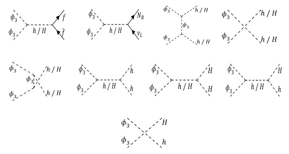
  Figure 1: Feynman diagrams for annihilation processes of scalar DM $\phi_{3}$.

  where the $\langle\sigma_{\phi_{3}}v\rangle$ is the thermal averaged cross-section. The mathematical expression of cross section for each processes are given in Appendix A.1. Thermal evolution of the DM, together with the DM relic density computation requires the thermal-averaged annihilation cross-section as an input.

  For a non-relativistic regime, the whole process of calculating a thermal averaged cross-section boils down to $\langle\sigma v\rangle\equiv\sigma v$ Bauer:2017qwy through s-wave scattering analysis Gondolo:1990dk . Here $v$ is the relative velocity between two DM particles, given through $s=m_{\phi_{3}}^{2}v^{2}+4m_{\phi_{3}}^{2}$. Expanding the term $\sigma v$ in Taylor series for $x\gg 1$, i.e. in the non-relativistic limit, we get

  $$\langle\sigma v\rangle~{}=~{}\sigma_{0}~{}+~{}\frac{\sigma_{1}}{x},$$ (34)

  where, parameter $x=m_{\phi_{3}}/T$, T being the temperature of the thermal bath. In the case of light dark matter as is the case for the scalar DM here, the DM has the potential chances to be boosted. At the same time, one can also have a light DM which is not boosted, for which the thermal averaging mechanism is outlined above. We later show that, in the context of the model described above, $\phi_{3}$ can actually be produced through $\chi_{1}~{}\chi_{1}\rightarrow\phi_{3}~{}\phi_{3}$ process, which will lead to boosted DM due to kinematic factors. The effect of the boost is separately explored in the next section Sec. 4. Hence, considering the fact that $\phi_{3}$ here may or may not get enough velocity to become relativistic, we decide to go ahead with the most general thermal averaged cross section computation method. For the scalar DM $\phi_{3}$, the thermal averaged cross-section is given by,

  $${\langle\sigma v\rangle}_{\phi_{3}\phi_{3}\to SM}=\frac{x}{8m_{\phi_{3}}^{5}K_{2}^{2}\Bigl{(}x\Bigl{)}}~{}\int_{4m_{\phi_{3}}^{2}}^{\infty}~{}\sigma(s)_{\phi_{3}}\times(s-4m_{\phi_{3}}^{2})\sqrt{s}K_{1}\Bigl{(}\frac{x\sqrt{s}}{m_{\phi_{3}}}\Bigl{)}ds,$$ (35)

  where $K_{n}$ are modified Bessel functions of order n. In Eq. 33, we can scale the number density with respect to the total entropy of the Universe, $s$, to work with a quantity called comoving density $Y_{i}=n_{i}/s$ that evolves with respect to a parameter $x=m/T$, T being the temperature of the Universe. With this scaling the Boltzmann equations are modified as:

  $$\frac{dY_{\phi_{3}}}{dx} = -\frac{1}{x^{2}}\frac{s(m_{\phi_{3}})}{H(m_{\phi_{3}})}\langle\sigma v\rangle_{\phi_{3}\phi_{3}\to SM}(Y_{\phi_{3}}^{2}-Y_{\phi_{3},\rm eq}^{2})$$ (36)

  Notice that the lower limit of the integration over the CM energy is $4m_{\phi_{3}}^{2}$ for the thermal averaged cross-section. It means that the particular DM particle can not annihilate to a particle which has mass greater than the DM mass. The reason being the fact the cross-section of the DM annihilation contains a factor $\sqrt{s-4m_{i}^{2}}$, which ceases to be real when $m_{\rm DM}\leq m_{i}$, $m_{i}$ being the mass of $i$-th particle, that the DM pairs can annihilate to. Therefore, based on the constraint, only kinematically available annihilation channels will open for the light scalar DM $\phi_{3}$ annihilation.

• Fermion DM $\chi_{1}$
  For the vectorlike fermion component of the DM, the equation takes the form,

  $$\frac{dn_{\chi_{1}}}{dt}+3Hn_{\chi_{1}}=-\frac{1}{2}\langle\sigma_{\chi_{1}}v\rangle(n_{\chi_{1}}^{2}-n_{\chi_{1},\rm eq}^{2})$$ (37)

  Here $\sigma_{\chi_{1}}$ is the annihilation cross section of the fermionic dark matter with $\chi_{1}$ annihilating to the visible sector as:

  $$\sigma_{\chi_{1}}(s) = \sigma(s)_{\chi_{1}\chi_{1}\to f\bar{f}}+\sigma(s)_{\chi_{1}\chi_{1}\to N_{R}\nu_{L}}+\sigma(s)_{\chi_{1}\chi_{1}\to hh}+\sigma(s)_{\chi_{1}\chi_{1}\to ZZ}$$ (38)

  $$+ \sigma(s)_{\chi_{1}\chi_{1}\to W^{+}W^{-}}$$

  and $\langle\sigma_{\chi_{1}}v\rangle$ are the thermal averaged cross-section. The Feynman diagrams are presented in Fig. 2, and the cross-section of each annihilation processes are described in Appendix A.2.

  

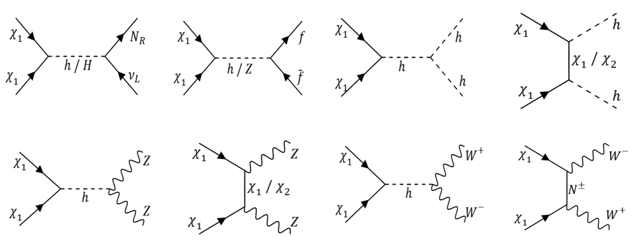
  Figure 2: Feynman diagrams for annihilation processes of fermionic DM $\chi_{1}$.

  Like the previous case, the thermal averaged cross-section of the fermionic DM, $\chi_{1}$ is given by,

  $${\langle\sigma v\rangle}_{\chi_{1}\chi_{1}\to SM}=\frac{x}{8m_{\phi_{3}}^{5}K_{2}^{2}\Bigl{(}x\Bigl{)}}~{}\int_{4m_{\chi_{1}}^{2}}^{\infty}~{}\sigma(s)_{\chi_{1}}\times(s-4m_{\chi_{1}}^{2})\sqrt{s}K_{1}\Bigl{(}\frac{x\sqrt{s}}{m_{\chi_{1}}}\Bigl{)}ds$$ (39)

  Scaling the number density with respect to the total entropy of the Universe, $s$, be defining a comoving density $Y_{\chi_{1}}=n_{\chi_{1}}/s$ and it’s evolution with respect to a parameter $x=m/T$, the modified Boltzmann equation for fermionic DM is modified to,

  $$\frac{dY_{\chi_{1}}}{dx} = -\frac{1}{2}\frac{1}{x^{2}}\frac{s(m_{\chi_{1}})}{H(m_{\chi_{1}})}\langle\sigma v\rangle_{\chi_{1}\chi_{1}\to SM}(Y_{\chi_{1}}^{2}-Y_{\chi_{1},\rm eq}^{2})$$ (40)

  where, the comoving number density at the equilibrium for the $i$-th particle is given by $Y_{i,eq}=0.145~{}\frac{g_{i}}{100}~{}x^{3/2}~{}e^{-x}$, with internal degrees of freedom $g_{i}=2$ for fermionic particles.
  

• Numerical Results
  The solution of the Boltzmann Equation for scalar DM (Eq. 36) and for fermionic DM (Eq. 40) candidates separately gives the Fig. 3 and Fig. 4 respectively. We show the freeze-out plot for one benchmark point with a fixed mass of both the DM candidates, $\phi_{3}$ and $\chi_{1}$. Solving Eq. 41 and following Eq. 43, we get the freeze out temperature, DM density at the freeze out and consequent relic abundance for the scalar DM $\phi_{3}$ and fermionic DM $\chi_{1}$ which are plotted in the right panel of Fig. 3 and 4 respectively. The relic abundance, can be expressed as Drees:2021rsg

  $$\Omega h^{2}=\frac{2.14\times 10^{9}~{}\rm{GeV^{-1}}}{\sqrt{g_{\ast}}~{}M_{pl}}\frac{1}{J(x_{f})}$$ (41)

  where $M_{\rm Pl}=1.22\times 10^{19}~{}\rm{GeV}$ is the Plank Mass and $J(x_{f})$ is given by

  $$J(x_{f})=\int_{x_{f}}^{\infty}~{}\frac{\langle\sigma v\rangle(x)}{x^{2}}~{}dx$$ (42)

  where $x_{f}=m/{T_{f}}$ with $T_{f}$ be the freeze-out temperature, obtained solving the Boltzmann equation governing DM thermal evolution.

  

  

  Figure 3: Left: Illustration of the freeze-out phenomenon for scalar dark matter $\phi_{3}$ annihilation from the thermal evolution using single Boltzmann equation. Right: Scalar dark matter relic density $\Omega_{\phi_{3}}h^{2}$ variation with the scalar DM mass $m_{\phi_{3}}$. The red band shows the relic density observed by the Plank experiment.

  In Fig. 3 we present the phenomenology of a scalar DM. In these plots, a single component Boltzmann Equation is solved for individual scalar DM $\phi_{3}$, to obtain the timeline and nature of freeze-out phenomenon for $\phi_{3}$. The left panel of Fig. 3 is drawn for different values of $m_{\phi_{3}}$, with other model parameters being fixed to particular benchmark values. We obtain the freeze-out phenomenon around $x\sim 15-20$, with the largest x obtained for a scalar dark matter mass $m_{\phi_{3}}\approx 10~{}$MeV. This is a sign of a relatively late freeze-out which happens due to enhanced annihilation, dominantly aided due to the DM mass being around the H-resonant region.

  The the right panel of Fig. 3, scalar DM relic density is shown with its variation as a function of scalar DM mass. The DM annihilation is enhanced by resonant $H$ mediated processes, leading to a resonant drop at $m_{\phi_{3}}\sim m_{H}/2$ in the relic density variation. The allowed relic density region is in the vicinity of $m_{\phi_{3}}\sim 10$ MeV for $m_{H}=20~{}$MeV. Relic density dip does not get much broader even as the resonant relic drop is followed by the onset of new t-channel $\phi_{3}\phi_{3}\to HH$ annihilation around $m_{\phi_{3}}\sim m_{H}$. Once these two annihilation processes continue to contribute with no new annihilation channels contributing anything significant, the relic density gradually increases with DM mass. The red band shows the 3$\sigma$ limit obtained from the experimentally measured of the relic density by the Planck collaboration Planck:2015fie .

  In Fig. 3 (right), the scalar DM mass $m_{\phi_{3}}\approx 100$ MeV produces the correct relic density according to the measurements. The resonance drop is due the $H$ mediated $s$ channel diagrams in the $\phi_{3}$ annihilation. Below 100 MeV, for most of the lower $m_{\phi_{3}}$ values relic density is under-abundant, while for DM masses higher than $m_{\phi_{3}}\approx 100~{}{\rm MeV}$ provide over abundant relic.

  From Eq. 43, following a non-relativistic approach for a heavy mass DM, the $\langle\sigma v\rangle$ is not a function of $x$. Therefore, the relic density expression for the fermionic DM becomes,

  $$\Omega h^{2}=\frac{2.14\times 10^{9}~{}x_{f}}{\sqrt{g_{\ast}}M_{pl}~{}\langle\sigma v\rangle}$$ (43)

  Using this, Eq. 41 and Eq. 43 are followed here to plot freeze-out diagrams and to find the relic density for the fermionic DM $\chi_{1}$ in Fig. 4.

  

  

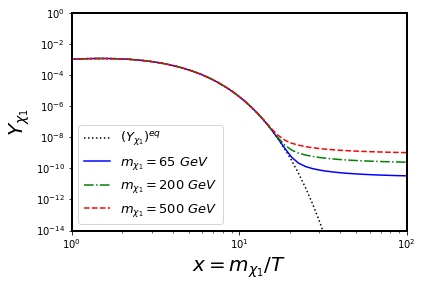
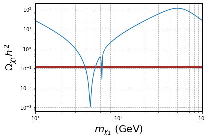
  Figure 4: Left: Solution of the Boltzmann Equation for the single component fermionic DM $\chi_{1}$, with showing freeze-out phenomenon for different masses of fermionic DM candidate $\chi_{1}$. Right: Fermionic DM relic density with the variation of fermionic DM mass. The grey band shows the correct relic density band measured by the Plank experiment.

  Scalar DM		Fermion DM
  Mass	Relic density	Mass	Relic density
  10 MeV	$2.75\times 10^{-6}$	45 GeV	0.001
  100 MeV	0.057	65 GeV	0.59
  1 GeV	39.16	200 GeV	17.16

  Table 4: The relic densities of the scalar and fermionic dark matter in single component scenario, showing their individual contributions corresponding to different dark matter masses.

  The relic density for the fermionic DM is shown by the Fig. 4 (right), where the two resonance drops in the relic density happen due to the contribution coming from the $Z$ and $h$ mediated $s$ channel diagrams respectively, with the $Z$ resonance drop being way more significant that the other. These two resonant drops at observed respectively at $m_{\chi_{1}}\sim m_{Z}/2$ and $m_{\chi_{1}}\sim m_{h}/2$ as evident from the Fig. 4 (right). Note, we have considered the Breit-Wigner resonance width of 2.5 GeV and 4 MeV for the $Z$ and $h$ bosons respectively. The relevant Feynman diagrams are shown in Fig. 2 and in Sec. A.2, we present the expression for the cross-section for each diagrams of the $\chi_{1}$ annihilation. A similar conclusion can be drawn from Fig. 4 where only a small region of fermionic DM, $\chi_{1}$ mass is allowed with an under abundant or exact relic density, touching the experimentally measured relic density band. The observations of Fig. 3, Fig. 4 are highlighted in Table 4 displaying a few points for different masses of $\phi_{3}$ and $\chi_{1}$ and their corresponding relic densities respectively.

3.2 Two Component Dark Matter: Coupled Boltzmann Equation

In the neutrinophilic model that is being explored here, the fermionic dark matter will be heavier and then it can annihilate to lighter scalar dark matter that we intend to analyze here. Their relic density together can be obtained only when we consider their number densities evolve through a set of coupled Boltzmann equations (CBE). The Boltzmann equations are expressed as:

$$\frac{dn_{\chi_{1}}}{dt}+3Hn_{\chi_{1}} = -\frac{1}{2}\langle\sigma_{\chi_{1}\chi_{1}\to\phi_{3}\phi_{3}}v\rangle(n_{\chi_{1}}^{2}-n_{\phi_{3}}^{2}\frac{n_{\chi_{1},\rm eq}^{2}}{n_{\phi_{3},\rm eq}^{2}})-\frac{1}{2}\langle\sigma_{\chi_{1}}v\rangle(n_{\chi_{1}}^{2}-n_{\chi_{1},\rm eq}^{2})$$

$$\frac{dn_{\phi_{3}}}{dt}+3Hn_{\phi_{3}} = -\langle\sigma_{\phi_{3}}v\rangle(n_{\phi_{3}}^{2}-n_{\phi_{3},\rm eq}^{2})-\langle\sigma_{\phi_{3}\phi_{3}\to\chi_{1}\chi_{1}}v\rangle(n_{\phi_{3}}^{2}-n_{\chi_{1}}^{2}\frac{n_{\phi_{3},\rm eq}^{2}}{n_{\chi_{1},\rm eq}^{2}})$$ (44)

Here $\sigma_{\chi_{1}\chi_{1}\to\phi_{3}\phi_{3}}$ (expression given in Appendix. 55) provides the cross-section of the fermionic DM annihilating to the scalar DM candidates, whereas $\sigma_{\phi_{3}\phi_{3}\to\chi_{1}\chi_{1}}$ provides the same for the reverse process. The $\chi_{1}\chi_{1}\to\phi_{3}\phi_{3}$ annihilation, which acts as the interaction term between the two DM candidates in our model, can be drawn as a Feynman diagram like Fig. 5. Here the $H$ mediated process is highly suppressed due to the very weak interaction strength of the H involved vertices $H\chi_{1}\chi_{1}$ and $H\phi_{3}\phi_{3}$ compared to those involving the SM Higgs, $h\chi_{1}\chi_{1}$ and $h\phi_{3}\phi_{3}$.

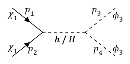
Figure 5: Higgs boson (h/H) mediated $\chi_{1}\chi_{1}\to\phi_{3}\phi_{3}$ annihilation diagram.

Scaling Eq. 44 with the comoving density $Y_{i}=n_{i}/s$ and the parameter $x\equiv x_{\phi_{3}}=m_{\phi_{3}}/T$ we get,

$$\frac{dY_{\chi_{1}}}{dx} = -\frac{1}{2}\frac{\lambda_{\chi\phi}}{x^{2}}\left(Y_{\chi_{1}}^{2}-Y_{\phi_{3}}^{2}\frac{Y_{\chi_{1},\rm eq}^{2}}{Y_{\phi_{3},\rm eq}^{2}}\right)-\frac{1}{2}\frac{\lambda_{\chi}}{x^{2}}\left(Y_{\chi_{1}}^{2}-Y_{\chi_{1},\rm eq}^{2}\right)$$

$$\frac{dY_{\phi_{3}}}{dx} = -\frac{\lambda_{\phi}}{x^{2}}\left(Y_{\phi_{3}}^{2}-Y_{\phi_{3},\rm eq}^{2}\right)+\frac{\lambda_{\chi\phi}}{x^{2}}\left(Y_{\chi_{1}}^{2}-Y_{\phi_{3}}^{2}\frac{Y_{\chi_{1},\rm eq}^{2}}{Y_{\phi_{3},\rm eq}^{2}}\right)$$

with

$$\lambda_{\chi\phi}=\frac{s(m_{\phi_{3}})}{H(m_{\phi_{3}})}\langle\sigma v\rangle_{\chi_{1}\chi_{1}\to\phi_{3}\phi_{3}}$$

,

$$\lambda_{\chi}=\frac{s(m_{\phi_{3}})}{H(m_{\phi_{3}})}\langle\sigma_{\chi_{1}}v\rangle\hskip 14.22636pt\lambda_{\phi}=\frac{s(m_{\phi_{3}})}{H(m_{\phi_{3}})}\langle\sigma_{\phi_{3}}v\rangle$$

where $s(m_{\phi_{3}})=\frac{2\pi^{2}}{45}g^{*}m_{\phi_{3}}^{3}$, $H(m_{\phi_{3}})=\frac{\pi}{90}\frac{\sqrt{g^{*}}}{M_{\rm Pl}}m_{\phi_{3}}^{2}$ with $g^{*}=106$ as the effective number of degrees of freedom and reduced plank mass $M_{\rm Pl}=2.44\times 10^{18}~{}{\rm GeV}$.

Solution of the coupled Boltzmann equation (CBE), i.e., Eq. LABEL:eq:cbe2, provides the freeze-out plots of the fermionic DM $\chi_{1}$ and the scalar DM $\phi_{3}$ together, where the $\langle\sigma v\rangle$ is the thermal averaged annihilation cross-section as discussed above. We implement the approximation $\langle\sigma v\rangle=\sigma\ v$ for the non-relativistic regime. This approximation is justified, because for a heavy mass dark matter, the fermionic one here, the parameter $x=m_{\chi_{1}}/T\gg 1$ is large and this is a non-relativistic limit. In the center of mass (CM) frame energy can be written in terms of the DM mass and $x$ parameter is $s=4m_{\chi_{1}}^{2}+2m_{\chi_{1}}^{2}/x$, and for $x\gg 1$, $s\approx 4~{}m_{\chi_{1}}^{2}$. Therefore the heavy mass of fermionic DM $\chi_{1}$ is the justified reason to take the non-relativistic limit in the calculation of $\langle\sigma_{\chi_{1}}v\rangle$. Based on the discussion in Eq. 34, we have taken $\langle\sigma_{\chi_{1}}v\rangle~{}=~{}\sigma_{0}+\sigma_{1}/x~{}\cong~{}\sigma_{0}$, with $x$ being very very large $\sigma_{0}\approx\sigma_{\chi_{1}}(s=4m_{\chi_{1}}^{2})$. In the two benchmark scenarios studied below we show a comparative analysis of individual dark matter candidates and two-component dark matter scenario, where the DM particles interact among each other.

The Figures in the left of the freeze-out diagrams of Scenario-I and II, depict the freeze-out for the individual fermionic DM $\chi_{1}$ and the scalar DM $\phi_{3}$ candidates, each one as a solution of the corresponding single component Boltzmann Equation (BE). The results show that a $\sim 45$ GeV fermionic DM can have an efficient resonant annihilation to have a relatively lower yield at the freeze-out, while at higher DM masses like $m_{\chi_{1}}\sim 200$GeV it goes to relic values that is over-abundant. For the scalar DM, relic density at freeze out will be relatively higher as the DM relic comes close to the measured number around $m_{\phi_{3}}\sim 20~{}$MeV, while it goes down to smaller values while exact resonance region is explored at $m_{\phi_{3}}\sim 10~{}$MeV.

Below plots shows the coupled two-component dark matter scenario for two different combinations of scalar and fermionic DM masses. For the two DM coupled cases, two x variables are possible: we choose $x=m_{\phi_{3}}/T$. It is observed that then the freeze-out phenomenon for the scalar and fermionic DM happens for very different x values, the fermion DM getting frozen out at a very smaller $x\sim 10^{-2}$ values while scalar DM freeze out happens at $x\sim 15$. Taking into effect the rescaling of $x$ for the heavier fermion DM, we observe that the freeze out happens almost at a similar era as the scalar one. Compared to the individual DM candidate case $x$ for the fermion DM sees a minor increase, which is an artefact of increased annihilation. The fermionic DM in this coupled sector has one additional mode to annihilate to which reduces the relic density, which is reflected in the lower DM yield. The dark matter yield for the fermionic DM decreases for both the cases with lower order of $Y_{\infty}$ ($Y_{\infty}=Y_{eq}(x_{f})$), compared to the individual DM scenarios. The scalar DM yield remains same albeit increases a bit in the coupled scenario. That happens because the scalar DM gets boosted being produced from the fermionic DM annihilation. This boost is not always sufficient enough to help the scalar DM to annihilate into new modes which was hitherto unavailable due to kinematic conditions. Due to the boost effects the s-channel resonant annihilation becomes less efficient which increases the relic.

• Scenario-I:

  

  

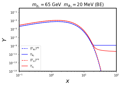
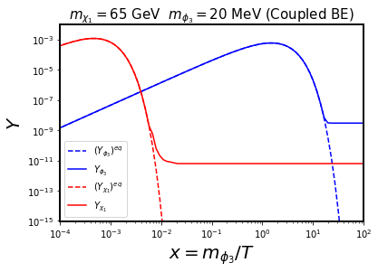
  Figure 6: Freeze-out plot for Coupled Boltzmann Equation (right panel) with $m_{\chi_{1}}=65~{}{\rm GeV}$ $m_{\phi_{3}}=20~{}{\rm MeV}$ and its comparison with the case of individual DM candidates (left panel).

  In this case (shown in Fig. 6) we take the fermionic DM mass in its Higgs mediated resonant annihilation region, where its individual relic density will be under-abundant albeit not in a way that happens in $Z$ resonance region. The scalar DM mass is taken as $m_{\phi_{3}}\sim 20$ MeV which is slightly away from the resonant region of $m_{H}/2\sim 10~{}$MeV, still with a relic density very close to the measured one. When we look at their individual dark matter phenomenology, the scalar DM freezes out at a smaller $x$ value with higher $Y_{\phi_{3}}$, even though the higher $Y_{\phi_{3}}$ could only manage to provide DM relic orders of magnitude lower than the fermionic DM here. For the fermionic DM, $Y_{\chi_{1}}$ is smaller by one order of magnitude, but results in a larger relic density.

  In the two component dark matter case using the coupled Boltzmann equation, the fermionic dark matter yield $Y_{\chi_{1}}$, decreases further due to its extra annihilation to the scalar DM channel. Even if the scalar DM is boosted, it does not gather enough energy to include any more significant annihilation channels. On the other hand its s-channel resonance contribution gets diluted due to a modified resonance condition in presence of a boost: so that its annihilation decreases and yield $Y_{\phi_{3}}$ increases further. This is reflected in the increased gap of the frozen out yield values for the fermionic and scalar DM cases in the coupled DM scenario. The fermionic contribution to the DM relic comes down in the coupled case compared to the individual fermionic DM case for the same mass. The scalar DM relic density increases to be at the same order of magnitude as the fermionic one, which is quite contrary to the individual DM case where their relic were far apart. Overall the total DM density goes down for a coupled DM case compared to the same scenario case with two individual DM candidates evolving through single Boltzmann equation, though still not enough to be under-abundant.

• Scenario-II:

  

  

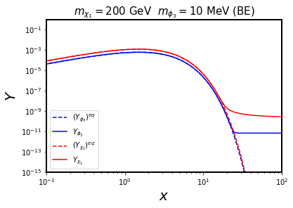
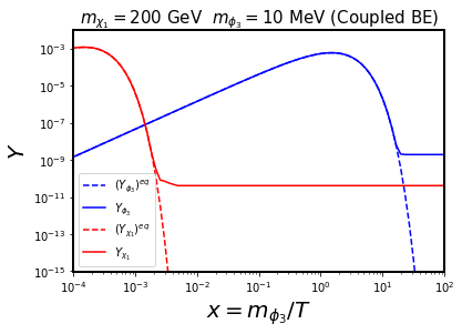
  Figure 7: Freeze-out plot for coupled Boltzmann equation (right panel) with $m_{\chi_{1}}=200~{}{\rm GeV}$ and $m_{\phi_{3}}=10~{}{\rm MeV}$, and its comparison with the case of individual DM candidates (left panel).

  In this case (shown in Fig. 7) we take the fermionic DM mass in a region where it is quiet away from the resonant region, which opens up the possibility of a higher yield of fermionic DM in the freeze out compared to the scenario-I. This is because the resonant contribution is absent in this VLL dark matter mass region; other annihilation contributions are not so significant. Here the fermionic DM relic density is over-abundant ($\sim 170$ times the observed relic density) when we take individual fermionic DM contribution. The scalar dark matter here stays exactly in the resonant region, where 20 MeV scalar $H$ mediated s-channel annihilation play dominant role. This makes the individual scalar DM relic density severely under-abundant to negligible values. This is reflected in the Fig. 7 (left) where even $Y_{\phi_{3}}$ freezes out at smaller values than the $Y_{\chi_{1}}$ which is completely opposite to what we get in the scenario-I.

Now we look at the relative importance of two dark matter components in the total relic density. Total relic abundance of the two-component DM scenario in this model-dependent study can be evaluated directly from the freeze-out plot using,

$$\Omega~{}h^{2}=\Omega_{\phi_{3}}h^{2}+\Omega_{\chi_{1}}h^{2}$$

, where $\Omega_{\phi_{3}}h^{2}$ and $\Omega_{\chi_{1}}h^{2}$ are computed as:

$$\Omega_{\phi_{3}}h^{2}~{}=~{}\frac{m_{\phi_{3}}~{}s_{0}~{}Y_{\phi_{3}}(\infty)}{\rho_{c}/h^{2}}\hskip 19.91684pt\Omega_{\chi_{1}}h^{2}=\frac{m_{\chi_{1}}~{}s_{0}~{}Y_{\chi_{1}}(\infty)}{\rho_{c}/h^{2}}$$ (46)

where $s_{0}=2890~{}{\rm cm^{-3}}$ is the current entropy density of the Universe and $\rho_{c}/h^{2}~{}=~{}1.05\times 10^{-5}~{}{\rm GeV/cm^{3}}$ is the critical density. The asymptotic value of $Y$’s, both $Y_{\phi_{3},\chi_{1}}(\infty)$ is the $Y_{\phi_{3},\chi_{1}}$ values computed at the freeze out point, that remains constant till date.

$m_{\chi_{1}}$ (GeV)	$m_{\phi_{3}}$ (MeV)	$\Omega_{\chi_{1}}h^{2}$	$\Omega_{\phi_{3}}h^{2}$	$\Omega h^{2}$
$65$	$20$	0.132	0.035	0.167
$65$	$100$	0.116	0.67	0.786
$65$	$1000$	0.105	277.8	277.9
$200$	$10$	9.35	0.00275	9.352
$200$	$100$	7.50	2.6	10.1
$200$	$1000$	4.13	345.09	349.22

Table 5: Tabulated form of the scalar and fermionic dark matter relic density in a coupled two component dark matter scenario, showing their relative contribution to the total relic density with their variation with the corresponding dark matter mass.

The results of the Fig. 6 and Fig. 7 are also shown numerically with variation of the relic density numbers with the DM mass. In Table 5, relic abundance numbers for both the dark matter candidates in the two-component dark matter coupled scenario, for the different masses of the fermionic DM and scalar DM, are tabulated showing their individual contribution to the total relic, listed separately along with the total relic density. From these values it can be concluded that only the $\chi_{1}$ masses around 50 GeV are able to produce under abundant relic density for both the scalar DM masses of 10 and 20 MeV. For the two component coupled scenario, the fermionic DM around 65-70 GeV case is the one that is able to satisfy the exact relic density.

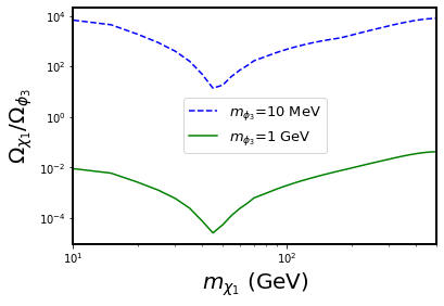
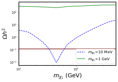
Figure 8: Left: Ratio of the abundances $\Omega_{\chi_{1}}/\Omega_{\phi_{3}}$ as a function of Fermion DM mass $m_{\chi_{1}}$ for two different scalar DM masses. Right: The total relic abundance $\Omega h^{2}=\Omega_{\phi_{3}}h^{2}+\Omega_{\chi_{1}}h^{2}$ as a function of fermion DM mass $m_{\chi_{1}}$. The red band shows the correct relic density band measured by the Planck experiment.

For the Fig. 8, we have scanned over the fermionic DM mass $m_{\chi_{1}}$ from 10 GeV to 500 GeV and compute total relic density summing up the contributions from both the fermionic and scalar DM components for a two component coupled DM scenario. We vary the fermion DM mass for the two cases with the scalar DM mass $m_{\phi_{3}}$ fixed at 10 MeV and 1 GeV respectively. We have also probed the relative importance of fermionic and scalar DM contributions in the total relic density. In the left plot, the ratio of the relic abundances $\Omega_{\chi_{1}}h^{2}$ and $\Omega_{\phi_{3}}h^{2}$ is shown as a function of fermionic dark matter mass $m_{\chi_{1}}$. Here $\Omega_{\phi_{3}}h^{2}$ and $\Omega_{\chi_{1}}h^{2}$ are respectively the relative contributions of the scalar and fermionic DM into the total DM relic density, when they are present together in the model. Over the full $m_{\chi_{1}}$ that is explored, accompanying scalar DM with two different masses lead to two completely opposite predictions. For a scalar DM with mass 10 MeV the fermionic component is dominant for the whole fermion DM mass range, with the scalar DM contributing less than 1% to 5% of the total relic. If the total DM behavior is studied for this scalar DM mass as shown in the Fig. 8 (right), observationally under-abundant or exact relic can be obtained upto fermion DM mass $m_{\chi_{1}}\sim 70~{}$GeV. This is an interesting modification in the fermion DM phenomenology as, a single component VLL DM was only viable in a narrow mass region $40-50$ GeV, which is now broadened upto $\sim 70$ GeV. This happens due to coupled nature of the DM sector, as a new annihilation channel for the fermionic DM opens up in the form $\chi_{1}\chi_{1}\to\phi_{3}\phi_{3}$. The grey solid band depicts the experimentally measured correct relic abundance within a $3\sigma$ range.

When the scalar DM mass is increased to 1 GeV, its relic density increases at par with the single scalar DM case, to gradually become the dominant component of total DM relic. Scalar DM is the dominant contributor to the dark matter relic, for all the fermionic DM masses explored here, reducing the fermionic contribution to at best of (3-4)% for $m_{\chi_{1}}\sim 1~{}$TeV and then decreasing further to all the lower DM values with below 1% contribution around $m_{\chi_{1}}\sim 45~{}$GeV. This is a significant deviation from the case where individual DM candidates are studied. In that case, for $m_{\chi_{1}}\geq 100~{}$GeV the relic was always higher than a 1 GeV scalar DM relic. With the boost the light scalar DM getting in the case of coupled DM scenario, the effect of resonance fades away even more for a 1 GeV scalar DM, which makes its annihilation less efficient and therefore results in higher relic.

To summarize, when the total DM relic is either under abundant or exact being compatible with the experimental measurements, the fermionic DM contribution always dominates the scalar one. Obviously there is parameter region where the scalar DM contribution is way greater than the fermionic counterpart. But in that scenario, total relic density is always over abundant i.e. ruled out by the experimental measurement.

4 Boost Effects in Dark Matter Phenomenology

In this paper we choose a two component dark matter scenario and the model satisfy the correct relic density for some specific values of the model parameters, as we have explained in the previous section. We have also found very different behavior of the scalar DM in one component and two component scenarios. The interplay of the scalar and vectorlike dark matter changes the properties of the DM candidates in the two component scenario. In the two component model, the light scalar DM obtains a boost which comes naturally from the annihilation $\chi_{1}\chi_{1}\to\phi_{3}\phi_{3}$. But before addressing that, let us first discuss the boost of a single component scalar dark matter. The annihilation processes have been discussed in the previous section already.

In the single component DM scenario ($\phi_{3}$), the DM can be boosted due to astrophysical phenomena such as collision due to cosmic rays etc. In such cases, the boost ($\gamma$) of the DM can be a free parameter and it is defined as,

$$\gamma_{\phi_{3}}=\frac{1}{\sqrt{1-v_{\phi_{3}}^{2}}}$$ (47)

The COM energy in the annihilation processes is expressed as

$$s=~{}4m_{\phi_{3}}^{2}+4m_{\phi_{3}}^{2}v_{\phi_{3}}^{2}.$$ (48)

In the presence of boosting effect, the COM energy increased due to the second term. As a result, the lower limit of the integration for the thermal averaged cross-section also change with the new COM energy. Therefore, additional annihilation channels opens up for $\phi_{3}$, even at the lower masses. The effect of additional annihilation channels will add up in the total cross-section. Hence for larger boost, the relic density will be higher. We plot the relic density of a single component scalar DM as a function of it’s mass for different boost ($\gamma_{\phi_{3}}$) in Fig.9. We also plot the no boost scenario, that is, $\gamma_{\phi_{3}}=0$ which is represented by the blue line. After the resonance drop at $m_{\phi_{3}}=m_{H}/2$ we get the broader region because the $t$ channel $\phi_{3}\phi_{3}\to HH$ process opens up. Interestingly, inclusion of the boost shifts the resonance drop towards left.

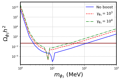
Figure 9: Variation of the relic density of the scalar DM with its mass for single component scalar DM scenario is shown. The blue line corresponds to the situation with no boost, $\gamma_{\phi_{3}}=0$. The red and green line represents two cases with arbitrary values of the boost. The red horizontal line represents the correct relic band as measured by Planck experiment.

Now let us discuss the boost effect in the two component scenario. The scalar DM achieves boost via the annihilation process $\chi_{1}\chi_{1}\to\phi_{3}\phi_{3}$. From the relativistic kinematic computation we obtain the the boosted velocity of the scalar DM as:

$$v_{\phi_{3}}^{2} = 1-\frac{m_{\phi_{3}}^{2}}{m_{\chi_{1}}^{2}}~{}(1-v_{\chi_{1}}^{2})\quad{\rm and~{}the~{}boost}\quad\gamma_{\phi_{3}}\sim\frac{m_{\chi_{1}}}{m_{\phi_{3}}}$$

The COM energy is expressed as

$$s=~{}4m_{\phi_{3}}^{2}+4m_{\phi_{3}}^{2}~{}\big{(}1-\frac{m_{\phi_{3}}^{2}}{m_{\chi_{1}}^{2}}~{}(1-v_{\chi_{1}}^{2})\big{)}$$ (49)

Note that, here the boosted COM energy $s$ is now a function of $m_{\phi_{3}}$ and $m_{\chi_{1}}$. We choose $v_{\chi_{1}}=~{}220~{}{\rm Km/s}$ according to the Maxwell-Boltzmann distribution of the DM velocity distribution in Standard Halo Model (SHM) Evans:2005tn ; Zemp:2008gw . In Fig.10 (Left) we show the DM relic density as a function of the scalar DM mass for two Benchmark masses of the vectorlike dark matter. The blue line shows the no boost scenario, as before. Here the scalar and the vectorlike dark matter together satisfy the total DM density as discussed in the previous section or in other words, the scalar DM satisfies only a fraction of the total DM density. When the vectorlike DM mass is 65 GeV, the Total relic is satisfied in this We also show in Fig.10 (Right) that a significant amount of boost can be achieved in our benchmark cases and the amount of boost increases with the mass of the vectorlike DM.

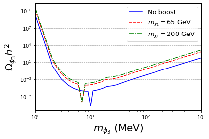
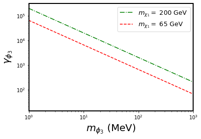
Figure 10: Left: The relic density of the boosted scalar DM as a function of its mass is shown for two benchmark values of the vectorlike DM. The blue solid line is the relic density of the scalar DM in the single component case with no boost. Right: The boost of the scalar DM and its variation with the scalar mass is shown for two benchmark values of the vectorlike DM in the two component scenario.

In Fig.10 (Left), the boost changes at every point of the plot as it depends on the masses of the scalar and the vectorlike dark matter. Thus, even if Fig.10 (Left) and Fig.9 look almost similar, the boost of the scalar DM is not similar in the two cases. In the two component model, correct relic density is achievable if the scalar DM mass and vectorlike DM mass are in the window 5-35 MeV and 35-60 GeV respectively. For these masses, the boost factor of the scalar around $\mathcal{O}({10^{3}})$. Note that this is only true for the particular benchmark points that we choose in this model. A slight variation in the couplings of the vectorlike DM changes these limits. From Table 5 in the previous section and Fig.10, it is clear that for the scalar DM mass around 10 MeV and vectorlike DM mass $\leq 65$ GeV the relic density is exact and under abundant, also a significant boost is achieved. Even higher boost is achievable for larger masses of the vectorlike DM, however, this tends to make the total relic to be overabundant in the particular benchmark points of the model parameters that we have chosen.

Detection Prospects of MeV scale Boosted DM

For the Scalar Dark matter, the strongest constraints are by XENON1T ⁸B XENON:2020gfr and PandaX-4T ⁸B PandaX:2022aac in the limit 4-10 GeV. Other experiments such as XENON1T XENON:2018voc , XENONnT XENONCollaboration:2023orw , PandaX-4T PandaX-4T:2021bab impose constraints on the spin-independent cross-section when mass of the dark matter is more than 10 GeV. However, the strongest limit comes from the LZ LUX-ZEPLIN:2022xrq experiment. Dark matter direct detection searches become challenging in the lower mass region and thus a because the threshold for nuclear recoil energy is very low. Hence in the lower mass region, the strong limit comes from the electron scattering experiments such as DarkSide DarkSide:2018bpj , PICO-60 PICO:2017tgi ; PICO:2019vsc and CRESST CRESST:2019jnq and a series of other projects. In Earth-based direct detection experiments, the dark matter particle interacts with either the nucleon or the electron of the atom. After the collision, the electron or the nucleon is recoiled with the energy transferred from the incoming dark matter particles. This recoil energy is then detected and measured by the experiments. If the mass of the DM particle is small (sub-GeV) it produces very small recoil energy, if not sufficiently boosted. On the other hand, if the DM travels with large amount of kinetic energy, small mass DM can transfer large amount of energy to the recoil electron ($\phi_{3}e^{-}\rightarrow\phi_{3}e^{-}$) or nucleon ($\phi_{3}n\rightarrow\phi_{3}n$).

The existing limits on the scalar DM can alter significantly if the particle is boosted. We discuss the effect of boost on the scalar DM $\phi_{3}$ in detail and it is shown that in the two component scenario, the MeV scale dark matter that satisfies the total relic density together with the VLDM, is $\sim 10$ MeV. For MeV scale DM in this range, sufficient amount of boost can be obtained which can overcome the detector thresholds. There are challenges in the detection the boosted Dark Matter in direct detection experiments. First of all, the flux of the boosted DM particle is small and nearly mono-energetic (Agashe:2015xkj, ). Hence for boosted dark matter, large volume detectors are preferred. We aim to discuss the detection prospect of the MeV scalar dark matter in detail in an upcoming work.

5 Summary and Discussions

In summary, we have arranged a low-mass scalar DM and a comparatively heavy-mass fermionic DM candidate in a modified $\nu 2HDM$ scenario and discuss the DM phenomenology in the context of relic density. In the $\nu 2HDM$ discussed here, there is one light CP even neutral scalar ($\approx 20~{}{\rm MeV}$) in addition to right-handed (RH) neutrinos $N_{R_{i}}$. One gauge singlet neutral scalar $\phi_{3}$ is added to the model which is stabilized to be the DM under the $Z_{2}$ symmetry. The vector-like lepton Lagrangian $L_{VLL}$ leads to one vector-like doublet ($N$) and one vector-like singlet ($\chi$). Mixing of the vector-like doublet ($N$) and vector-like singlet ($\chi$) gives the second DM candidate of our model i.e. the fermionic DM $\chi_{1}$. The Yukawa sector of the $2HDM$ contains the interaction of the SM fermions with the Higgs bosons. Along with other constraints, the oblique parameters could have constrained the model because of the light scalar $H$, but the addition of vector-like doublet and singlet do allow for more favorable parameter space. After imposing different constraints such as Higgs and $Z$ boson invisible widths, stability of the potential etc, we choose the benchmark points from the allowed region of the parameter space.

In this model, both the DM candidates annihilate to different SM particles, aided by s-channel resonant processes, along with some t-channel contributions. The Higgs (also the CP even scalar $H$) mediated channels play a dominant role for both the DM candidates in this scenario. Boltzmann equations are constructed to assess thermal evolution of both the DM candidates: first individually for them and then in a coupled DM scenario. To construct the Boltzmann Equation, thermal averaged cross sections are used as inputs. Thermal averaging of a cross-section is re-explained in both the relativistic and non-relativistic regimes. In the process of thermal-averaging of the cross-section, the limits on mandelstam parameter $s$ is found to be important to distinguish between relativistic and non-relativistic approaches. First we analyze the freeze out of the scalar and fermionic DM in the uncoupled scenario. We find that the fermionic DM is very restricted while a light DM is somewhat favorable from context of the relic density. Even then the scalar DM cannot be detected due to its inability to do nuclear/electron recoils. Then we consider the coupled scenario, where we have solved the CBE (Coupled Boltzmann Equation ) for the DM particles. The cross-term in the CBE allows for additional annihilation channels for the fermion DM, and this is reflected in the delayed freeze-out of the fermion DM. On the other hand, for the scalar DM the s-channel resonant condition gets diluted, leading to less effective DM annihilation. Scalar DM relic density gets enhanced to allow for smaller mass range of [5-35] MeV. Therefore, we have found that the DM candidates satisfy the correct relic abundance for $m_{\chi_{1}}\approx[35-60]~{}{\rm GeV}$ for different $m_{\phi_{3}}$ values around $10-20$ MeV.

The choice of a light MeV scalar DM and a heavy fermionic DM, is crucial to have a boosted DM in two component DM scenario. The fermionic DM is said to be non-relativistic with an rms velocity $\approx 220~{}{\rm Km/s}$ in the galactic halo. But due to the heavy mass, it can annihilate to $\phi_{3}$ (based on our study), and the energy conservation rule-wise the $\phi_{3}$ gets huge kinetic energy. We observe that the boost received from the $\chi_{1}\chi_{1}\to\phi_{3}\phi_{3}$ annihilation is equivalent to a relativistic factor $\gamma\sim[10^{3}-10^{4}]$. One crucial observation in our work is that the boosted light DM relic density phenomenology is almost independent of how it is boosted. The allowed $\phi_{3}$ DM mass range gets curtailed from the stand alone scalar DM, whether boost is obtained in the coupled scenario or from any other sources. This boosted DM has special importance in the DM direct detection study, where a DM candidate hits a detector-level particle (electron or nucleon) and generates the electron recoil energy $E_{e}$ or the nucleon recoil energy $E_{NR}$, which is detected by the detector. Therefore, a more energetic DM candidate (DM with boost) will produce more recoil energy, and thus the possibility of its detection gets enhanced. In our future work, we discuss the direct detection prospects of MeV scale light scalar DM, which is boosted from heavier fermionic DM. As both the DM candidates in the two component model interacts with the SM, the future study in the detection prospect of the light dark matter will shed new light in the DM physics here.

Appendix A Dark Matter Annihilation cross sections

A.1 Scalar DM annihilation diagrams and cross sections

• $\phi_{3}\phi_{3}\rightarrow f\bar{f}$

  $$\sigma(s)_{\phi_{3}\phi_{3}\rightarrow f\bar{f}} = \frac{1}{16\pi s}\frac{\sqrt{s-4m_{f}^{2}}~{}(s-4m_{f}^{2})}{\sqrt{s-4m_{\phi_{3}}^{2}}}\Bigg{[}\frac{\lambda_{\phi_{3}\phi_{3}h}^{2}~{}\lambda_{ffh}^{2}}{(s-m_{h}^{2})^{2}}$$ (50)

  $$+ \frac{\lambda_{\phi_{3}\phi_{3}H}^{2}~{}\lambda_{ffH}^{2}}{(s-m_{H}^{2})^{2}}$$

  $$+ \frac{2\lambda_{\phi_{3}\phi_{3}h}~{}\lambda_{ffh}\lambda_{\phi_{3}\phi_{3}H}~{}\lambda_{ffH}}{(s-m_{h}^{2})(s-m_{H}^{2})}\Bigg{]}$$

• $\phi_{3}\phi_{3}\rightarrow N_{R}\;\nu_{L}$

  $$\sigma(s)_{\phi_{3}\phi_{3}\to N_{R}\nu_{L}} = \frac{1}{16\pi s}\frac{\sqrt{s-m_{N_{R}}^{2}}~{}(s-m_{N_{R}}^{2})}{\sqrt{s-4m_{\phi_{3}}^{2}}}\Bigg{[}\frac{\lambda_{\phi_{3}\phi_{3}h}^{2}~{}\lambda_{h\nu_{L}N_{R}}^{2}}{(s-m_{h}^{2})^{2}}$$ (51)

  $$+ \frac{\lambda_{\phi_{3}\phi_{3}H}^{2}~{}\lambda_{H\nu_{L}N_{R}}^{2}}{(s-m_{H}^{2})^{2}}$$

  $$+ \frac{2~{}\lambda_{\phi_{3}\phi_{3}h}~{}\lambda_{\phi_{3}\phi_{3}H}~{}\lambda_{h\nu_{L}N_{R}}~{}\lambda_{H\nu_{L}N_{R}}}{(s-m_{h}^{2})(s-m_{H}^{2})}\Bigg{]}$$

• $\phi_{3}\phi_{3}\;\rightarrow\;hh$

  $$\sigma(s)_{\phi_{3}\phi_{3}\to hh} = \frac{(\lambda_{\phi_{3}\phi_{3}h})^{4}}{\pi s}\frac{\sqrt{s-4m_{h}^{2}}}{\sqrt{s-4m_{\phi_{3}}^{2}}}\frac{1}{4m_{h}^{4}-16m_{h}^{2}m_{\phi_{3}}^{2}+4sm_{\phi_{3}}^{2}}+\frac{1}{16\pi s}\frac{\sqrt{s-4m_{h}^{2}}}{\sqrt{s-4m_{\phi_{3}}^{2}}}\Bigg{[}(\lambda_{\phi_{3}\phi_{3}}^{hh})^{2}$$

  $$+ \frac{(\lambda_{\phi_{3}\phi_{3}h}~{}\lambda_{hhh})^{2}}{(s-m_{h}^{2})^{2}}+\frac{(\lambda_{\phi_{3}\phi_{3}H}~{}\lambda_{hhH})^{2}}{(s-m_{H}^{2})^{2}}+\frac{2\lambda_{\phi_{3}\phi_{3}}^{hh}\lambda_{\phi_{3}\phi_{3}h}\lambda_{hhh}}{(s-m_{h}^{2})}$$

  $$+ \frac{2\lambda_{\phi_{3}\phi_{3}}^{hh}\lambda_{\phi_{3}\phi_{3}H}\lambda_{hhH}}{(s-m_{H}^{2})}+\frac{2\lambda_{\phi_{3}\phi_{3}h}\lambda_{hhh}~{}\lambda_{\phi_{3}\phi_{3}H}~{}\lambda_{hhH}}{(s-m_{h}^{2})(s-m_{H}^{2})}\Bigg{]}$$

  $$+ \log\frac{2m_{h}^{2}-s+\sqrt{s-4m_{\phi_{3}}^{2}}\sqrt{s-4m_{h}^{2}}}{2m_{h}^{2}-s-\sqrt{s-4m_{\phi_{3}}^{2}}~{}\sqrt{s-4m_{h}^{2}}}\Bigg{[}\frac{\lambda_{\phi_{3}\phi_{3}}^{hh}(\lambda_{\phi_{3}\phi_{3}h})^{2}}{4\pi s(s-4m_{\phi_{3}}^{2})}$$

  $$+ \frac{(\lambda_{\phi_{3}\phi_{3}h})^{3}\lambda_{hhh}}{4\pi s(s-4m_{\phi_{3}}^{2})(s-m_{h}^{2})}+\frac{(\lambda_{\phi_{3}\phi_{3}h})^{2}\lambda_{\phi_{3}\phi_{3}H}\lambda_{hhH}}{4\pi s(s-4m_{\phi_{3}}^{2})(s-m_{H}^{2})}\Bigg{]}$$

• $\phi_{3}\phi_{3}\;\rightarrow\;HH$

  $$\sigma(s)_{\phi_{3}\phi_{3}\to HH} = \frac{(\lambda_{\phi_{3}\phi_{3}H})^{4}}{\pi s}\frac{\sqrt{s-4m_{H}^{2}}}{\sqrt{s-4m_{\phi_{3}}^{2}}}\frac{1}{4m_{H}^{4}-16m_{H}^{2}m_{\phi_{3}}^{2}+4sm_{\phi_{3}}^{2}}+\frac{1}{16\pi s}\frac{\sqrt{s-4m_{H}^{2}}}{\sqrt{s-4m_{\phi_{3}}^{2}}}\Bigg{[}(\lambda_{\phi_{3}\phi_{3}}^{HH})^{2}$$

  $$+ \frac{(\lambda_{\phi_{3}\phi_{3}H}\lambda_{HHH})^{2}}{(s-m_{H}^{2})^{2}}+\frac{(\lambda_{\phi_{3}\phi_{3}h}~{}\lambda_{hHH})^{2}}{(s-m_{h}^{2})^{2}}+\frac{2\lambda_{\phi_{3}\phi_{3}}^{HH}\lambda_{\phi_{3}\phi_{3}H}~{}\lambda_{HHH}}{(s-m_{H}^{2})}$$

  $$+ \frac{2\lambda_{\phi_{3}\phi_{3}}^{HH}\lambda_{\phi_{3}\phi_{3}h}\lambda_{hHH}}{(s-m_{h}^{2})}+\frac{2\lambda_{\phi_{3}\phi_{3}h}\lambda_{HHH}\lambda_{\phi_{3}\phi_{3}H}\lambda_{hHH}}{(s-m_{h}^{2})(s-m_{H}^{2})}\Bigg{]}$$

  $$+ \log\frac{2m_{H}^{2}-s+\sqrt{s-4m_{\phi_{3}}^{2}}\sqrt{s-4m_{H}^{2}}}{2m_{H}^{2}-s-\sqrt{s-4m_{\phi_{3}}^{2}}\sqrt{s-4m_{H}^{2}}}\Bigg{[}\frac{\lambda_{\phi_{3}\phi_{3}}^{HH}(\lambda_{\phi_{3}\phi_{3}H})^{2}}{4\pi s(s-4m_{\phi_{3}}^{2})}$$

  $$+ \frac{(\lambda_{\phi_{3}\phi_{3}H})^{3}\lambda_{HHH}}{4\pi s(s-4m_{\phi_{3}}^{2})(s-m_{H}^{2})}+\frac{(\lambda_{\phi_{3}\phi_{3}H})^{2}\lambda_{\phi_{3}\phi_{3}h}\lambda_{hHH}}{4\pi s(s-4m_{\phi_{3}}^{2})(s-m_{h}^{2})}\Bigg{]}$$

• $\phi_{3}\phi_{3}\;\rightarrow\;hH$

  $$\sigma(s)_{\phi_{3}\phi_{3}\to hH} = \frac{1}{16\pi s}\frac{\sqrt{s-(m_{h}+m_{H})^{2}}}{\sqrt{s-4m_{\phi_{3}}^{2}}}\Bigg{[}~{}\frac{(\lambda_{\phi_{3}\phi_{3}h}~{}\lambda_{hhH})^{2}}{(s-m_{h}^{2})^{2}}+\frac{(\lambda_{\phi_{3}\phi_{3}H}~{}\lambda_{hHH})^{2}}{(s-m_{H}^{2})^{2}}+(\lambda_{\phi_{3}\phi_{3}}^{hH})^{2}$$

  $$+ \frac{2\lambda_{\phi_{3}\phi_{3}h}~{}\lambda_{\phi_{3}\phi_{3}H}~{}\lambda_{hhH}~{}\lambda_{hHH}}{(s-m_{h}^{2})(s-m_{H}^{2})}+\frac{2\lambda_{\phi_{3}\phi_{3}}^{hH}~{}\lambda_{\phi_{3}\phi_{3}h}~{}\lambda_{hhH}}{(s-m_{h}^{2})}+\frac{2\lambda_{\phi_{3}\phi_{3}}^{hH}~{}\lambda_{\phi_{3}\phi_{3}H}~{}\lambda_{hHH}}{(s-m_{H}^{2})}~{}\Bigg{]}$$

A.2 Fermionic DM annihilation diagrams and cross sections

• $\chi_{1}\;\chi_{1}\rightarrow\;\phi_{3}\;\phi_{3}$

  $$\sigma_{\chi_{1}\chi_{1}\to\phi_{3}\phi_{3}} = \frac{1}{16\pi}\;\frac{\sqrt{s-4m_{\phi_{3}}^{2}}}{\sqrt{s-4m_{\chi_{1}}^{2}}}\Bigg{[}\frac{(\lambda_{\chi_{1}\chi_{1}h}~{}\lambda_{\phi_{3}\phi_{3}h})^{2}}{(s-m_{h}^{2})^{2}}+\frac{(\lambda_{\chi_{1}\chi_{1}H}~{}\lambda_{\phi_{3}\phi_{3}H})^{2}}{(s-m_{H}^{2})^{2}}$$ (55)

  $$+ \frac{\lambda_{\chi_{1}\chi_{1}h}~{}\lambda_{\phi_{3}\phi_{3}h}~{}\lambda_{\chi_{1}\chi_{1}H}~{}\lambda_{\phi_{3}\phi_{3}H}}{(s-m_{h}^{2})(s-m_{H}^{2})}\Bigg{]}$$

• $\chi_{1}\chi_{1}\rightarrow f\bar{f}$

  $$\sigma(s)_{\chi_{1}\chi_{1}\to f\bar{f}} = \frac{(\lambda_{\chi_{1}\chi_{1}h~{}\lambda_{hf\bar{f}}})^{2}~{}(s-4m_{f}^{2})^{3/2}}{4\pi\big{(}(s-m_{h}^{2})^{2}+{\Gamma_{h}^{2}m_{h}^{2}}\big{)}\sqrt{s-4m_{\chi_{1}}^{2}}}~{}+\frac{\lambda_{\chi_{1}\chi_{1}Z}^{2}\sqrt{s-4m_{f}^{2}}}{4\pi s\sqrt{s-4m_{\chi_{1}}^{2}}~{}\big{(}(s-M_{Z}^{2})^{2}+\Gamma_{Z}^{2}M_{Z}^{2}\big{)}}$$ (56)

  $$\times \Bigg{[}\frac{1}{3}(c_{A}^{2}+c_{V}^{2})(4s^{2}+16m_{f}^{2}m_{\chi}^{2}-4s(m_{\chi}^{2}+m_{f}^{2}))$$

  $$+ 2m_{\chi}^{2}(c_{A}^{2}+c_{V}^{2})(s-2m_{f}^{2})+2m_{f}^{2}s(c_{A}^{2}-c_{V}^{2})\Bigg{]}$$

• $\chi_{1}\chi_{1}\rightarrow N_{R}\nu_{L}$

  $$\sigma(s)_{\chi_{1}\chi_{1}\to N_{R}\nu_{L}} = \frac{1}{16\pi}\frac{\sqrt{s-m_{N_{R}}^{2}}(s-m_{N_{R}}^{2})}{\sqrt{s-4m_{\chi_{1}}^{2}}}\Bigg{[}\frac{(\lambda_{\chi_{1}\chi_{1}H}~{}\lambda_{HN_{R}\nu_{L}})^{2}}{(s-m_{H}^{2})^{2}}+\frac{(\lambda_{\chi_{1}\chi_{1}h}\lambda_{hN_{R}\nu_{L}})^{2}}{(s-m_{h}^{2})^{2}}$$ (57)

  $$+ \frac{\lambda_{\chi_{1}\chi_{1}H}~{}\lambda_{\chi_{1}\chi_{1}h}~{}\lambda_{HN_{R}\nu_{L}}~{}\lambda_{hN_{R}\nu_{L}}}{(s-m_{h}^{2})~{}(s-m_{H}^{2})}\Bigg{]}$$

• $\chi_{1}~{}\chi_{1}\;\rightarrow\;h~{}h~{}$(t channel)

  $$\sigma(s)_{\chi_{1}\chi_{1}\to hh} = \frac{\lambda_{\chi_{1}\chi_{1}h}^{4}}{\pi(s-4m_{\chi_{1}}^{2})}~{}\Bigg{[}\frac{8m_{\chi_{1}}^{2}\sqrt{s-4m_{\chi_{1}}^{2}}\sqrt{s-4m_{h}^{2}}}{4m_{h}^{4}-16m_{h}^{2}m_{\chi_{1}}^{2}+4sm_{\chi_{1}}^{2}}-\log\frac{2m_{h}^{2}-s-\sqrt{s-4m_{\chi_{1}}^{2}}\sqrt{s-4m_{h}^{2}}}{2m_{h}^{2}-s+\sqrt{s-4m_{\chi_{1}}^{2}}\sqrt{s-4m_{h}^{2}}}\Bigg{]}$$ (58)

  $$+ \frac{\lambda_{\chi_{1}\chi_{2}h}^{4}}{\pi(s-4m_{\chi_{1}}^{2})}\Bigg{[}~{}\frac{4(m_{\chi_{1}}^{2}+m_{\chi_{2}}^{2})\sqrt{s-4m_{\chi_{1}}^{2}}\sqrt{s-4m_{h}^{2}}}{(2m_{\chi_{1}}^{2}-2m_{\chi_{2}}^{2}+2m_{h}^{2}-s)^{2}-(s-4m_{\chi_{1}}^{2})(s-4m_{h}^{2})}$$

  $$- \log\frac{2m_{\chi_{1}}^{2}+2m_{h}^{2}-2m_{\chi_{2}}^{2}-s-\sqrt{s-4m_{\chi_{1}}^{2}}\sqrt{s-4m_{h}^{2}}}{2m_{\chi_{1}}^{2}+2m_{h}^{2}-2m_{\chi_{2}}^{2}-s+\sqrt{s-4m_{\chi_{1}}^{2}}\sqrt{s-4m_{h}^{2}}}\Bigg{]}+\frac{\lambda_{\chi_{1}\chi_{1}h}^{2}\lambda_{hhh}^{2}}{8\pi(s-m_{h}^{2})^{2}}\frac{\sqrt{s-4m_{h}^{2}}}{\sqrt{s-4m_{\chi_{1}}^{2}}}$$

  $$+ \frac{\lambda_{\chi_{1}\chi_{1}h}^{2}~{}\lambda_{\chi_{1}\chi_{2}h}^{2}}{\pi(s-4m_{\chi_{1}}^{2})}~{}\Bigg{[}\log\frac{2m_{\chi_{1}}^{2}+2m_{h}^{2}-2m_{\chi_{2}}^{2}-s+\sqrt{s-4m_{\chi_{1}}^{2}}\sqrt{s-4m_{h}^{2}}}{2m_{\chi_{1}}^{2}+2m_{h}^{2}-2m_{\chi_{2}}^{2}-s-\sqrt{s-4m_{\chi_{1}}^{2}}\sqrt{s-4m_{h}^{2}}}+\frac{2m_{\chi_{1}}^{2}}{(m_{\chi_{1}}^{2}-m_{\chi_{2}}^{2})}$$

  $$\times \Bigg{[}\log\frac{2m_{h}^{2}-s+\sqrt{s-4m_{\chi_{1}}^{2}}\sqrt{s-4m_{h}^{2}}}{2m_{h}^{2}-s-\sqrt{s-4m_{\chi_{1}}^{2}}\sqrt{s-4m_{h}^{2}}}$$

  $$- \log\frac{2m_{\chi_{1}}^{2}+2m_{h}^{2}-2m_{\chi_{2}}^{2}-s+\sqrt{s-4m_{\chi_{1}}^{2}}\sqrt{s-4m_{h}^{2}}}{2m_{\chi_{1}}^{2}+2m_{h}^{2}-2m_{\chi_{2}}^{2}-s-\sqrt{s-4m_{\chi_{1}}^{2}}\sqrt{s-4m_{h}^{2}}}\Bigg{]}\Bigg{]}$$

  $$+ \frac{\lambda_{\chi_{1}\chi_{1}h}\lambda_{hhh}~{}m_{\chi_{1}}}{4\pi(s-m_{h}^{2})(s-4m_{\chi_{1}}^{2})}\Bigg{[}\lambda_{\chi_{1}\chi_{1}h}^{2}\log\frac{2m_{h}^{2}-s+\sqrt{s-4m_{\chi_{1}}^{2}}\sqrt{s-4m_{h}^{2}}}{2m_{h}^{2}-s-\sqrt{s-4m_{\chi_{1}}^{2}}\sqrt{s-4m_{h}^{2}}}$$

  $$+ \lambda_{\chi_{1}\chi_{2}h}^{2}\log\frac{2m_{\chi_{1}}^{2}+2m_{h}^{2}-2m_{\chi_{2}}^{2}-s+\sqrt{s-4m_{\chi_{1}}^{2}}\sqrt{s-4m_{h}^{2}}}{2m_{\chi_{1}}^{2}+2m_{h}^{2}-2m_{\chi_{2}}^{2}-s-\sqrt{s-4m_{\chi_{1}}^{2}}\sqrt{s-4m_{h}^{2}}}\Bigg{]}$$

• $\chi_{1}~{}\chi_{1}\;\rightarrow\;Z~{}Z~{}$

  $$\sigma(s)_{\chi_{1}\chi_{1}\to ZZ} = \frac{\sqrt{s-4m_{Z}^{2}}}{16\pi\sqrt{s-4m_{\chi_{1}}^{2}}}\Bigg{[}\frac{\lambda_{\chi_{1}\chi_{1}Z}^{4}(12m_{Z}^{4}+s^{2}-4sm_{Z}^{2})}{m_{Z}^{2}(m_{Z}^{4}-4m_{Z}^{2}m_{\chi_{1}}^{2}+sm_{\chi_{1}}^{2})}+\frac{(\lambda_{\chi_{1}\chi_{1}h}~{}\lambda_{hZZ})^{2}(12m_{Z}^{4}+s^{2}-4sm_{Z}^{2})}{(s-m_{h}^{2})^{2}~{}4m_{Z}^{4}}$$ (59)

  $$+ \frac{\lambda_{\chi_{1}\chi_{2}Z}^{4}(12m_{Z}^{4}+s^{2}-4sm_{Z}^{2})}{m_{Z}^{2}\Big{(}(2m_{\chi_{1}}^{2}+2m_{h}^{2}-2m_{\chi_{2}}^{2}-s)^{2}-(s-4m_{\chi_{1}}^{2})(s-4m_{Z}^{2})\Big{)}}\Bigg{]}$$

  $$+ \frac{1}{16\pi}\frac{\lambda_{\chi_{1}\chi_{1}h}~{}\lambda_{hZZ}~{}m_{\chi_{1}}}{(s-4m_{\chi_{1}}^{2})(s-m_{h}^{2})m_{Z}^{4}}\Bigg{[}\lambda_{\chi_{1}\chi_{1}Z}^{2}(12m_{Z}^{4}+s^{2}-4sm_{Z}^{2})$$

  $$\times \log\frac{2m_{Z}^{2}-s+\sqrt{s-4m_{Z}^{2}}\sqrt{s-4m_{\chi_{1}}^{2}}}{2m_{Z}^{2}-s-\sqrt{s-4m_{Z}^{2}}\sqrt{s-4m_{\chi_{1}}^{2}}}$$

  $$+ \lambda_{\chi_{1}\chi_{2}Z}^{2}(12m_{Z}^{4}+s^{2}-4sm_{Z}^{2})\log\frac{2m_{\chi_{1}}^{2}+2m_{Z}^{2}-2m_{\chi_{2}}^{2}-s+\sqrt{s-4m_{Z}^{2}}\sqrt{s-4m_{\chi_{1}}^{2}}}{2m_{\chi_{1}}^{2}+2m_{Z}^{2}-2m_{\chi_{2}}^{2}-s-\sqrt{s-4m_{Z}^{2}}\sqrt{s-4m_{\chi_{1}}^{2}}}\Bigg{]}$$

  $$+ \frac{\lambda_{\chi_{1}\chi_{1}Z}^{2}\lambda_{\chi_{1}\chi_{2}Z}^{2}}{16\pi}\frac{12m_{Z}^{4}+s^{2}-4sm_{Z}^{2}}{m_{z}^{2}(s-4m_{\chi_{1}}^{2})(m_{\chi_{1}}^{2}-m_{\chi_{2}}^{2})}\Bigg{[}\log\frac{2m_{Z}^{2}-s+\sqrt{s-4m_{Z}^{2}}\sqrt{s-4m_{\chi_{1}}^{2}}}{2m_{Z}^{2}-s-\sqrt{s-4m_{Z}^{2}}\sqrt{s-4m_{\chi_{1}}^{2}}}$$

  $$- \log\frac{2m_{\chi_{1}}^{2}+2m_{Z}^{2}-2m_{\chi_{2}}^{2}-s+\sqrt{s-4m_{Z}^{2}}\sqrt{s-4m_{\chi_{1}}^{2}}}{2m_{\chi_{1}}^{2}+2m_{Z}^{2}-2m_{\chi_{2}}^{2}-s-\sqrt{s-4m_{Z}^{2}}\sqrt{s-4m_{\chi_{1}}^{2}}}\Bigg{]}$$

• $\chi_{1}~{}\chi_{1}\;\rightarrow\;W^{+}~{}W^{-}$

  $$\sigma(s)_{\chi_{1}\chi_{1}\to W^{+}W^{-}}=\frac{\sqrt{s-4m_{W}^{2}}}{4\pi\sqrt{s-4m_{\chi_{1}}^{2}}}~{}\Bigg{[}\frac{(\lambda_{\chi_{1}\chi_{1}h}~{}\lambda_{hW^{+}W^{-}})^{2}(12m_{W}^{4}+s^{2}-4sm_{W}^{2})}{16m_{W}^{2}(s-m_{h}^{2})^{2}}$$

  $$+\frac{\lambda_{\chi_{1}N_{-}W^{+}}^{2}\lambda_{\chi_{1}N_{+}W^{-}}^{2}~{}(12m_{W}^{4}+s^{2}-4sm_{W}^{2})}{m_{W}^{2}(4m_{\chi_{1}}^{4}+4m_{W}^{4}+m_{N}^{4}-4m_{\chi_{1}}^{2}m_{N}^{2}-4m_{W}^{2}m_{N}^{2}-8m_{\chi_{1}}^{2}m_{W}^{2}+2m_{N}^{2}s)}\Bigg{]}$$

  $$+\frac{1}{16\pi}\frac{(\lambda_{\chi_{1}\chi_{1}h}~{}\lambda_{hW^{+}W^{-}}~{}\lambda_{\chi_{1}N_{-}W^{+}}~{}\lambda_{\chi_{1}N_{+}W^{-}})~{}m_{\chi_{1}}~{}(12m_{W}^{4}+s^{2}-4sm_{W}^{2})}{(s-4m_{\chi_{1}}^{2})~{}(s-m_{h}^{2})~{}4m_{W}^{4}}$$

  $$\times\log\frac{2m_{\chi_{1}}^{2}+2m_{W}^{2}-m_{N}^{2}-s+\sqrt{s-4m_{W}^{2}}\sqrt{s-4m_{\chi_{1}}^{2}}}{2m_{\chi_{1}}^{2}+2m_{W}^{2}-m_{N}^{2}-s-\sqrt{s-4m_{W}^{2}}\sqrt{s-4m_{\chi_{1}}^{2}}}$$ (60)

References

- (1) F. Zwicky, Die Rotverschiebung von extragalaktischen Nebeln, Helv. Phys. Acta 6 (1933) 110.
- (2) K.G. Begeman, A.H. Broeils and R.H. Sanders, Extended rotation curves of spiral galaxies: Dark haloes and modified dynamics, Mon. Not. Roy. Astron. Soc. 249 (1991) 523.
- (3) J. Silk et al., Particle Dark Matter: Observations, Models and Searches, Cambridge Univ. Press, Cambridge (2010), 10.1017/CBO9780511770739.
- (4) M. Bauer and T. Plehn, Yet Another Introduction to Dark Matter: The Particle Physics Approach, vol. 959 of Lecture Notes in Physics, Springer (2019), 10.1007/978-3-030-16234-4, [1705.01987].
- (5) G. Bertone, D. Hooper and J. Silk, Particle dark matter: Evidence, candidates and constraints, Phys. Rept. 405 (2005) 279 [hep-ph/0404175].
- (6) M. Lisanti, Lectures on Dark Matter Physics, in Theoretical Advanced Study Institute in Elementary Particle Physics: New Frontiers in Fields and Strings, pp. 399–446, 2017, DOI [1603.03797].
- (7) Planck collaboration, Planck 2015 results. XIII. Cosmological parameters, Astron. Astrophys. 594 (2016) A13 [1502.01589].
- (8) K.M. Zurek, Multi-Component Dark Matter, Phys. Rev. D 79 (2009) 115002 [0811.4429].
- (9) S. Bhattacharya, N. Chakrabarty, R. Roshan and A. Sil, Multicomponent dark matter in extended : neutrino mass and high scale validity, JCAP 04 (2020) 013 [1910.00612].
- (10) DAMA collaboration, First results from DAMA/LIBRA and the combined results with DAMA/NaI, Eur. Phys. J. C 56 (2008) 333 [0804.2741].
- (11) XENON collaboration, Excess electronic recoil events in XENON1T, Phys. Rev. D 102 (2020) 072004 [2006.09721].
- (12) XENON collaboration, Search for New Physics in Electronic Recoil Data from XENONnT, Phys. Rev. Lett. 129 (2022) 161805 [2207.11330].
- (13) Planck Collaboration, Aghanim, N., Akrami, Y., Ashdown, M., Aumont, J., Baccigalupi, C. et al., Planck 2018 results - vi. cosmological parameters, A&A 641 (2020) A6.
- (14) G. Arcadi, M. Dutra, P. Ghosh, M. Lindner, Y. Mambrini, M. Pierre et al., The waning of the WIMP? A review of models, searches, and constraints, Eur. Phys. J. C 78 (2018) 203 [1703.07364].
- (15) XENON collaboration, Search for Coherent Elastic Scattering of Solar 8B Neutrinos in the XENON1T Dark Matter Experiment, Phys. Rev. Lett. 126 (2021) 091301 [2012.02846].
- (16) T. Bringmann and M. Pospelov, Novel direct detection constraints on light dark matter, Phys. Rev. Lett. 122 (2019) 171801 [1810.10543].
- (17) A. Das and M. Sen, Boosted dark matter from diffuse supernova neutrinos, Phys. Rev. D 104 (2021) 075029 [2104.00027].
- (18) C. Xia, Y.-H. Xu and Y.-F. Zhou, Azimuthal asymmetry in cosmic-ray boosted dark matter flux, Phys. Rev. D 107 (2023) 055012 [2206.11454].
- (19) C.A. Argüelles, A. Kheirandish and A.C. Vincent, Imaging Galactic Dark Matter with High-Energy Cosmic Neutrinos, Phys. Rev. Lett. 119 (2017) 201801 [1703.00451].
- (20) S. Bhowmick, D. Ghosh and D. Sachdeva, Blazar boosted dark matter — direct detection constraints on e: role of energy dependent cross sections, JCAP 07 (2023) 039 [2301.00209].
- (21) J.-W. Wang, A. Granelli and P. Ullio, Direct Detection Constraints on Blazar-Boosted Dark Matter, Phys. Rev. Lett. 128 (2022) 221104 [2111.13644].
- (22) A. Granelli, P. Ullio and J.-W. Wang, Blazar-boosted dark matter at Super-Kamiokande, JCAP 07 (2022) 013 [2202.07598].
- (23) T.N. Maity and R. Laha, Cosmic-ray boosted dark matter in Xe-based direct detection experiments, 2210.01815.
- (24) D. Bardhan, S. Bhowmick, D. Ghosh, A. Guha and D. Sachdeva, Bounds on boosted dark matter from direct detection: The role of energy-dependent cross sections, Phys. Rev. D 107 (2023) 015010 [2208.09405].
- (25) K. Agashe, Y. Cui, L. Necib and J. Thaler, (In)Direct Detection of Boosted Dark Matter, J. Phys. Conf. Ser. 718 (2016) 042041 [1512.03782].
- (26) G. Belanger and J.-C. Park, Assisted freeze-out, JCAP 03 (2012) 038 [1112.4491].
- (27) M. Dutta, S. Mahapatra, D. Borah and N. Sahu, Self-interacting Inelastic Dark Matter in the light of XENON1T excess, Phys. Rev. D 103 (2021) 095018 [2101.06472].
- (28) D. Borah, M. Dutta, S. Mahapatra and N. Sahu, Boosted self-interacting dark matter and XENON1T excess, Nucl. Phys. B 979 (2022) 115787 [2107.13176].
- (29) S. Baek, Inelastic dark matter, small scale problems, and the XENON1T excess, JHEP 10 (2021) 135 [2105.00877].
- (30) P. Ko, C.-T. Lu and U. Min, Crossing two-component dark matter models and implications for 511 keV -ray and XENON1T excesses, 2202.12648.
- (31) W. Grimus, L. Lavoura, O.M. Ogreid and P. Osland, A Precision constraint on multi-Higgs-doublet models, J. Phys. G 35 (2008) 075001 [0711.4022].
- (32) W. Grimus, L. Lavoura, O.M. Ogreid and P. Osland, The Oblique parameters in multi-Higgs-doublet models, Nucl. Phys. B 801 (2008) 81 [0802.4353].
- (33) H.E. Haber and D. O’Neil, Basis-independent methods for the two-Higgs-doublet model III: The CP-conserving limit, custodial symmetry, and the oblique parameters S, T, U, Phys. Rev. D 83 (2011) 055017 [1011.6188].
- (34) P.A.N. Machado, Y.F. Perez, O. Sumensari, Z. Tabrizi and R.Z. Funchal, On the Viability of Minimal Neutrinophilic Two-Higgs-Doublet Models, JHEP 12 (2015) 160 [1507.07550].
- (35) T. Nomura and H. Okada, Neutrinophilic two Higgs doublet model with dark matter under an alternative gauge symmetry, Eur. Phys. J. C 78 (2018) 189 [1708.08737].
- (36) S. Mohanty and S. Sadhukhan, Explanation of IceCube spectrum with neutrino splitting in a 2HDM model, JHEP 10 (2018) 111 [1802.09498].
- (37) S.A.R. Ellis, R.M. Godbole, S. Gopalakrishna and J.D. Wells, Survey of vector-like fermion extensions of the Standard Model and their phenomenological implications, JHEP 09 (2014) 130 [1404.4398].
- (38) M. Drees and W. Zhao, for light dark matter, , the 511 kev excess and the hubble tension, Phys. Lett. B 827 (2022) 136948 [2107.14528].
- (39) G.C. Branco, P.M. Ferreira, L. Lavoura, M.N. Rebelo, M. Sher and J.P. Silva, Theory and phenomenology of two-Higgs-doublet models, Phys. Rept. 516 (2012) 1 [1106.0034].
- (40) E. Ma, Naturally small seesaw neutrino mass with no new physics beyond the TeV scale, Phys. Rev. Lett. 86 (2001) 2502 [hep-ph/0011121].
- (41) T. Binder, S. Chakraborti, S. Matsumoto and Y. Watanabe, A global analysis of resonance-enhanced light scalar dark matter, JHEP 01 (2023) 106 [2205.10149].
- (42) CMS collaboration, A search for decays of the Higgs boson to invisible particles in events with a top-antitop quark pair or a vector boson in proton-proton collisions at = 13 TeV, 2303.01214.
- (43) H. Bahl, T. Biekötter, S. Heinemeyer, C. Li, S. Paasch, G. Weiglein et al., HiggsTools: BSM scalar phenomenology with new versions of HiggsBounds and HiggsSignals, Comput. Phys. Commun. 291 (2023) 108803 [2210.09332].
- (44) CMS collaboration, Precision measurement of the Z boson invisible width in pp collisions at s=13 TeV, Phys. Lett. B 842 (2023) 137563 [2206.07110].
- (45) ALEPH, DELPHI, L3, OPAL, LEP collaboration, Search for Charged Higgs bosons: Combined Results Using LEP Data, Eur. Phys. J. C 73 (2013) 2463 [1301.6065].
- (46) O. Seto, Large invisible decay of a Higgs boson to neutrinos, Phys. Rev. D 92 (2015) 073005 [1507.06779].
- (47) E. Bertuzzo, Y.F. Perez G., O. Sumensari and R. Zukanovich Funchal, Limits on Neutrinophilic Two-Higgs-Doublet Models from Flavor Physics, JHEP 01 (2016) 018 [1510.04284].
- (48) M. Sher and C. Triola, Astrophysical Consequences of a Neutrinophilic Two-Higgs-Doublet Model, Phys. Rev. D 83 (2011) 117702 [1105.4844].
- (49) M.E. Peskin and T. Takeuchi, Estimation of oblique electroweak corrections, Phys. Rev. D 46 (1992) 381.
- (50) E.W. Kolb and M.S. Turner, The Early Universe, vol. 69 (1990), 10.1201/9780429492860.
- (51) P. Gondolo and G. Gelmini, Cosmic abundances of stable particles: Improved analysis, Nucl. Phys. B 360 (1991) 145.
- (52) N.W. Evans and J.H. An, Distribution function of the dark matter, Phys. Rev. D 73 (2006) 023524 [astro-ph/0511687].
- (53) M. Zemp, J. Diemand, M. Kuhlen, P. Madau, B. Moore, D. Potter et al., The Graininess of Dark Matter Haloes, Mon. Not. Roy. Astron. Soc. 394 (2009) 641 [0812.2033].
- (54) PandaX collaboration, Search for Solar B8 Neutrinos in the PandaX-4T Experiment Using Neutrino-Nucleus Coherent Scattering, Phys. Rev. Lett. 130 (2023) 021802 [2207.04883].
- (55) XENON collaboration, Dark Matter Search Results from a One Ton-Year Exposure of XENON1T, Phys. Rev. Lett. 121 (2018) 111302 [1805.12562].
- (56) (XENON Collaboration)††, XENON collaboration, First Dark Matter Search with Nuclear Recoils from the XENONnT Experiment, Phys. Rev. Lett. 131 (2023) 041003 [2303.14729].
- (57) PandaX-4T collaboration, Dark Matter Search Results from the PandaX-4T Commissioning Run, Phys. Rev. Lett. 127 (2021) 261802 [2107.13438].
- (58) LUX-ZEPLIN collaboration, First Dark Matter Search Results from the LUX-ZEPLIN (LZ) Experiment, Phys. Rev. Lett. 131 (2023) 041002 [2207.03764].
- (59) DarkSide collaboration, Low-Mass Dark Matter Search with the DarkSide-50 Experiment, Phys. Rev. Lett. 121 (2018) 081307 [1802.06994].
- (60) PICO collaboration, Dark Matter Search Results from the PICO-60 C3F8 Bubble Chamber, Phys. Rev. Lett. 118 (2017) 251301 [1702.07666].
- (61) PICO collaboration, Dark Matter Search Results from the Complete Exposure of the PICO-60 C3F8 Bubble Chamber, Phys. Rev. D 100 (2019) 022001 [1902.04031].
- (62) CRESST collaboration, First results from the CRESST-III low-mass dark matter program, Phys. Rev. D 100 (2019) 102002 [1904.00498].