BIPP: An efficient HPC implementation of the Bluebild algorithm for radio astronomy

Abstract

The Bluebild algorithm is a new technique for image synthesis in radio astronomy which forms a least-squares estimate of the sky intensity function using the theory of sampling and interpolation operators. We present an HPC implementation of the Bluebild algorithm for radio-interferometric imaging: Bluebild Imaging++ (BIPP). BIPP is a spherical imager that leverages functional PCA to decompose the sky into distinct energy levels. The library features interfaces to C++, C and Python and is designed with seamless GPU acceleration in mind. We evaluate the accuracy and performance of BIPP on simulated observations of the upcoming Square Kilometer Array Observatory and real data from the Low-Frequency Array (LOFAR) telescope. We find that BIPP offers accurate wide-field imaging with no need for a w-term approximation and has comparable execution time with respect to the interferometric imaging libraries CASA  and WSClean. Futhermore, due to the energy level decomposition, images produced with BIPP can reveal information about faint and diffuse structures before any cleaning iterations. The source code of BIPP is publicly released.

1 Introduction

Radio astronomers are engaged in ambitious new projects to detect faster, fainter, and more distant astrophysical phenomena. The flagship project is the Square Kilometer Array Observatory (SKAO) (Dewdney et al., 2009), a next-generation radio astronomy facility that will revolutionize our understanding of the Universe and the laws of fundamental physics.

The SKAO is one of the major “Big Data” challenges of the next decade. According to the SKA estimates (Broekema et al., 2015), the Science Data Processor (SDP) workflow will need to be able to deal with a data flow rate of around 1 TB/s at full capacity. The SKAO will require a supercomputer of around 100 Pflops to transform the data before it is sent to the regional centres around the world for storage and final analysis by scientists. A major task of the SDP workflow will be reconstructing images of the sky from radio signals recorded across all array elements. However, image formation is a complicated problem.

The goal of image synthesis in radio astronomy is to reconstruct an estimate of the sky intensity function $I$ from finite measurements of visibility space $V\in\mathbb{C}^{L\times L}$. The state-of-the art radio-interferometry imaging software such as WSClean (Offringa et al., 2014) use the CLEAN family of algorithms (Högbom, 1974), which back project the visibilities into the image domain to create the “dirty” image of the sky. Then, assuming a point-source model, the algorithms deconvolve iteratively to extract a final “clean” image of the sky. However, these algorithms will struggle to meet the requirements of SKA: they often require thousands of iterations on the same data to converge. Additionally, the increased sensitivity and resolution of the SKAO imply that future observations may have more complex structure distributions across the field of view than simple point source fields. Thus, next-generation imaging algorithms will not only have to cope with large data but also leverage more complex signal models or become entirely model-agnostic.

One option is the Bluebild algorithm (Kashani, 2017), an imager based on the theory of sampling and interpolation operators (Vetterli et al., 2014), which produces a least-squares consistent image of the sky. Image formation is formulated as a continuous inverse problem, and a key innovation of Bluebild is to use functional PCA (fPCA) decomposition to simplify calculations of the sky image.

Using the Bluebild algorithm as part of an imaging pipeline has the following advantages:

• It incorporates instrument knowledge to construct a least-squares estimate of the sky, which the dirty image only approximates.

• It naturally incorporates spherical imaging, making it very suitable for wide field of view imaging.

• It performs a functional PCA decomposition of the sky, thus producing several images of varying energy levels rather than a single one, facilitating new analysis techniques.

• As we show, it can be implemented with comparable runtime as dirty image generation using CASA or WSClean.

In this paper, we provide a brief overview of the Bluebild algorithm and present our HPC implementation BIPP: Bluebild Imaging++. We show extensive validation results, comparing the output of BIPP to WSClean  and CASA (McMullin et al., 2007), and evaluate the performance of the BIPP library. Finally, we explore the effect of the fPCA decomposition on image reconstruction and discuss scientific applications and future directions.

2 The Bluebild Algorithm

For a full discussion and derivation of the Bluebild algorithm, we refer the reader to Kashani (2017) and Matthieu Simeoni (In preparation).

Over a single frequency, let the sky emissions we wish to observe be described by a continuous complex distribution $S(\vec{r})$, where $\vec{r}$ is a (unit) direction vector. A radio antenna $l$ with gain $g_{l}(\vec{r})$ will measure a voltage $x_{l}$ given by (Simeoni & Hurley, 2019):

$$x_{l}=\int_{S^{2}}S(\vec{r})~{}g_{l}(\vec{r})~{}\phi_{l}(\vec{r})~{}d\Omega~{},$$ (1)

where $\phi_{l}(\vec{r})\equiv\exp{\bigr{(}-\frac{2\pi i}{\lambda}\langle\vec{p}_{l},\vec{r}\rangle\bigl{)}}$ is the steering vector of the instrument and $\vec{p}_{l}$ is the instantaneous antenna position. If we sample $S(\vec{r})$ using a grid of ($N_{\mathrm{pixel}}$,3) International Celestial Reference System (ICRS) coordinates $\vec{x}_{p}$, we get a discrete form of Eq. 1:

$$x_{l}=\sum_{p}^{N_{\mathrm{pixel}}}S_{p}~{}g_{lp}~{}e^{-\frac{2\pi i}{\lambda}\langle\vec{p}_{l},\vec{x}_{p}\rangle}=\sum_{p}^{N_{\mathrm{pixel}}}\Psi^{*}_{lp}S_{p}~{},$$ (2)

where $\Psi^{*}\in\mathbb{C}^{L\times N_{\mathrm{pixel}}}$ is a matrix known as the sampling operator, which defines a mapping from the $N_{\mathrm{pixel}}$ sky coordinates $\vec{x}_{\mathrm{pix}}$ to the $L$ antenna indices.

The correlation between antennas is then given by the visibility matrix $V\in\mathbb{C}^{L\times L}$ (van der Veen & Wijnholds, 2013):

$$V_{lm}\equiv\mathbb{E}[x_{l}~{}x^{*}_{m}]=\sum^{N_{\mathrm{pixel}}}_{p}\sum^{N_{\mathrm{pixel}}}_{q}\Psi^{*}_{lp}~{}\mathbb{E}[S_{p}~{}S_{q}^{*}]~{}\Psi_{mq}~{}.$$ (3)

This is the discrete version of the radio interferometer measurement equation (RIME) (Hamaker et al., 1996; Rau et al., 2009; Smirnov, 2011). We can also write Equation 5 more compactly in matrix form:

$$V=\Psi^{*}~{}B~{}\Psi,$$ (4)

where $B\in\mathbb{C}^{N_{\mathrm{pixel}}\times N_{\mathrm{pixel}}}$ denotes the covariance matrix of the discretized sky emission $S$.

Because signals coming from different directions in the sky are uncorrelated (Taylor et al., 1999) we can write $B=\text{diag}(I)$, where $I_{p}=|S_{p}|^{2}$ is the diagonal of $B$. Visibilities can then be rewritten as:

$$V_{lm}=\sum^{N_{\mathrm{pixel}}}_{p}g_{lp}~{}I_{p}~{}g_{mp}^{*}~{}e^{-\frac{2\pi i}{\lambda}\langle\vec{p}_{lm},\vec{x}_{p}\rangle}~{},$$ (5)

where $\vec{p}_{lm}\equiv\vec{p}_{l}-\vec{p}_{m}$.

The least-squares covariance kernel $\widetilde{B}$ estimated by Bluebild is obtained by post-processing visibilities with a pseudo-inverse operator (Kashani, 2017). When written in discrete matrix form, this yields:

$$\widetilde{B}=\Psi G_{\Psi}^{-1}~{}V~{}G_{\Psi}^{-1}\Psi^{*}~{},$$ (6)

where $G_{\Psi}\in\mathbb{C}^{L\times L}$ is the Gram matrix of the instrument defined as $G_{\Psi}\equiv\Psi^{*}\Psi$. In the discrete formulation $G_{\Psi}$ is given by

$$(G_{\Psi})_{lm}=\langle\Psi_{l},\Psi_{m}\rangle=\sum_{p}^{N_{\mathrm{pixel}}}g_{lp}~{}g_{mp}^{*}~{}e^{-\frac{2\pi i}{\lambda}\langle\vec{p}_{lm},\vec{x}_{p}\rangle}~{}.$$ (7)

Note that the expression for the Gram matrix maps the instrument response in antenna indices. In the case of calibrated omnidirectional antennas we can write $g_{p}(\vec{r})=1$, and the Gram matrix can be shown to have the following analytical closed form (at the continuous level):

$$(G_{\Psi})_{lm}=\mathrm{sinc}~{}\Bigl{(}2~{}\Bigl{|}\Bigl{|}\frac{\vec{p}_{lm}}{\lambda}\Bigr{|}\Bigr{|}\Bigr{)}~{}.$$ (8)

Unfortunately, the Gram matrix can be ill-conditioned (Taylor, 1978), hence evaluating Eq. 6 is prone to error. One approach is to approximate the equation by setting the off-diagonal elements of $G_{\Psi}$ to zero, which reduces $G_{\Psi}$ to the identity matrix. Plugging this back into equation 6 and using $g_{p}(r)=1$ we obtain:

$$\widetilde{I}_{p}=\widetilde{B}_{pp}=\sum^{L}_{l}\sum^{L}_{m}V_{lm}~{}e^{\frac{2\pi i}{\lambda}\langle\vec{p}_{lm},\vec{x}_{p}\rangle}~{},$$ (9)

where $\widetilde{I}_{p}$ is our estimate of the sky intensity. By choosing an appropriate index $b$ for the baselines created by antenna pairs $l$ and $m$, this reduces to the expression for the non-uniform discrete Fourier transform of type 3 (Bagchi & Mitra, 1999):

$$\widetilde{I}_{p}=\sum_{b}^{L\times L}V_{b}~{}e^{-\frac{2\pi i}{\lambda}\langle\vec{p}_{b},\vec{x}_{p}\rangle}~{},$$ (10)

where $\vec{p}_{b}$ are the baselines, $V_{b}$ are the visibilities, and $\vec{x}_{p}$ are the Fourier frequencies.

Note that the familiar expression for the dirty image $I_{D}$ can be obtained by replacing the Gram matrix with the identity matrix, choosing a regular sampling of the sky pixels $x_{\mathrm{pix}}$ in $lmn$ coordinates while assuming negligible curvature of the sky ($\sqrt{1-l^{2}-m^{2}}\simeq 0$), and translating the antenna baselines $\vec{p}_{b}$ into the familiar $uvw$ frame:

$$I_{D}[l,m]=\sum_{u}\sum_{v}V[u,v]e^{-2\pi i(ul+vm)}~{},$$ (11)

where $V[u,v]$ is the map of samples in the $uv$ plane with sample positions given by the baseline vectors and sample strength given by $V$. Note that in the equation above, $(l,m)$ represent sky coordinates rather than antenna indices, as they do in the rest of this paper.

This dirty image is the starting point for current radio interferometry imaging software such as WSClean (Offringa et al., 2014). These algorithms calculate $I_{D}$, assume that all radio sources in the sky are point sources, and then iteratively subtract a distortion called the “dirty beam” around these points using the CLEAN family of algorithms (Högbom, 1974). However, they do not produce a least-squares estimate of the sky intensity. Many modern interferometers are implicitly designed such that the off-diagonal terms of the Gram matrix can be small, and the dirty image can be a reasonable approximation of the least-squares solution. However, for instruments with redundant baselines or low frequencies, the off-diagonal terms are larger, and the Gram matrix has a stronger effect.

2.1 Functional Principle Component Analysis

We want to calculate $\widetilde{B}$ and thus $\widetilde{I}$ from Equation 6 without using any approximations to ensure $\widetilde{B}$ always minimizes the least-squares optimization problem. Bluebild achieves this by directly finding a decomposition of $\widetilde{B}$ in a compact orthogonal basis, namely

$$\widetilde{B}=\sum_{a}\lambda_{a}\epsilon_{a}\epsilon_{a}^{H}=\sum_{a}\lambda_{a}\Psi\alpha_{a}\alpha_{a}^{H}\Psi^{*},$$ (12)

where $\{(\lambda_{a},\epsilon_{a}\equiv\Psi\alpha_{a})\}\in\mathbb{R}\times\mathbb{C}^{N_{\mathrm{pixel}}}$ are eigenpairs of $\widetilde{B}$. The relation $\epsilon_{a}=\Psi\alpha_{a}$, where $\alpha_{a}\in\mathbb{C}^{L}$ follows since $\epsilon_{a}\subset\text{span}(\Psi)$. The parameters $\{(\lambda_{a},\alpha_{a})\}$ can easily be inferred starting from the eigenvalue property:

$$\widetilde{B}\epsilon_{a}=\lambda_{a}\epsilon_{a}~{}.$$

Combining the above with the expression for $\widetilde{B}$ in Equation 6 and using $\epsilon_{a}\equiv\Psi\alpha_{a}$ we obtain:

$$\bigl{(}\Psi G_{\Psi}^{-1}~{}V~{}G_{\Psi}^{-1}\Psi^{*}\bigr{)}~{}\Psi\alpha_{a}=\lambda_{a}\Psi\alpha_{a}$$

Using $G_{\Psi}=\Psi^{*}\Psi$, this reduces to:

$$V\alpha_{a}=\lambda_{a}G_{\Psi}\alpha_{a}.$$ (13)

Thus the parameters $\{(\lambda_{a},\alpha_{a})\}$ are obtained by solving the generalized eigenvalue problem $V\alpha_{a}=\lambda_{a}G_{\Psi}\alpha_{a}$. This allows us to calculate the least-squares solution without inverting $G_{\Psi}$, giving:

$$\widetilde{I}=\sum_{a}\lambda_{a}|\epsilon_{a}|^{2}=\sum_{a}\lambda_{a}|\Psi\alpha_{a}|^{2}~{}.$$ (14)

The eigenvalue decomposition can be computed in $\mathcal{O}(L^{3})$ operations, where $L$ is the number of beams or dishes in the interferometer. The computational cost of the decomposition does not contribute significantly to the overall computation time because $L$ remains small. Indeed, SKA-Mid in South Africa is expected to have $L=197$ dishes, and SKA-Low in Australia is expected to have $L=512$ stations.

2.2 Image Synthesis

2.2.1 Standard Image Synthesis

After obtaining our eigenpairs $(\lambda_{a},\alpha_{a})$, we can reconstruct $\epsilon_{a}$ by applying $\Psi$:

$$\epsilon_{ap}=\sum_{l}\Psi_{pl}\alpha_{al}=\sum_{l}e^{\frac{2\pi i}{\lambda}\langle\vec{p}_{l},\vec{x}_{p}\rangle}\alpha_{al}~{}.$$ (15)

Directly calculating this result via matrix multiplication is called Standard Synthesis.

Radio interferometers typically collect data for hours, averaging the voltage data down into discrete timesteps. Because $\vec{p}_{l}$ is comprised of the instantaneous antenna positions, $\Psi$ is a time-dependent operator which must be evaluated at each timestep.

2.2.2 NUFFT Image Synthesis

We can improve Standard Synthesis by levering algorithms for the type 3 non-uniform FFT (Lee & Greengard, 2005). The expression for our least-squares reconstructed sky can be expanded as

$$\widetilde{I}=\sum_{a}\lambda_{a}|\epsilon_{a}|^{2}=\Psi~{}V^{\prime}~{}\Psi^{*}~{},$$ (16)

where $V^{\prime}$ are the Gram-corrected visibilities

$$V^{\prime}=\alpha_{a}~{}\mathrm{diag}(\lambda_{a})~{}\alpha_{a}^{H}~{}.$$ (17)

By rewriting the antenna indices $l,m$ into one baseline index $b$, we can write Equation 16 in the form of the type 3 non-uniform FFT to reconstruct the least-squares estimate of the sky (Kashani et al., 2023):

$$\widetilde{I}_{p}=\sum_{n}^{N}V^{\prime}_{n}e^{i\langle b_{n},x_{p}\rangle}~{},$$ (18)

where the $N$ samples of the visibilities $V^{\prime}_{n}$ correspond to coordinates $b_{n}$ in the $uvw$ plane. This allows us to stack the visibility samples across timesteps and perform only one call to NUFFT, greatly simplifying computational complexity with respect to Standard Synthesis.

2.3 Beamforming

For certain telescopes, the $L$ antenna samples $x_{l}$ are not available directly but are instead beamformed together into $K$ beams using a weighting matrix $W\in\mathbb{C}^{L\times K}$ (Æçal et al., 2015). The beamformed samples $x^{\prime}_{k}$ are then given by:

$$x^{\prime}_{k}=\sum_{l}W_{kl}^{*}x_{l}~{}.$$ (19)

Thus, the beamforming matrix $W$ defines a mapping between the $L$ antennas and $K$ stations. We can define a modified sampling operator, which includes beamforming $\Phi^{*}=W^{H}\Psi^{*}$. The beamformed visibilities $V^{W}\in\mathbb{C}^{K\times K}$ are thus given by:

$$V^{W}=\Phi^{*}~{}B~{}\Phi=W^{H}~{}\Psi^{*}~{}B~{}\Psi~{}W~{},$$ (20)

and with beamforming, the Gram matrix $G_{\Psi}^{W}\in\mathbb{C}^{K\times K}$ becomes:

$$G_{\Psi}^{W}=\Phi^{*}~{}\Phi=W^{H}~{}\Psi^{*}~{}\Psi~{}W~{}.$$ (21)

Beamforming can easily be accommodated in Standard Synthesis and NUFFT Synthesis with this redefined sampling operator.

2.4 Energy Levels & Partitioning

A key aspect of the Bluebild algorithm is decomposing the sky into distinct energy levels defined by $\{(\lambda_{a},\alpha_{a})\}$ pairs as shown in Equation 14. These levels can be manipulated via truncation, partitioning, or filtering to create different output images.

Truncation: not every eigenvector $\alpha_{a}$ needs to be used for constructing the LSQ sky intensity estimate $\widetilde{I}$. As the eigenvectors with the smallest eigenvalues often correspond to noise, BIPP includes an option only to construct images using $N_{\mathrm{eig}}\leq L$ leading eigenvectors. $N_{\mathrm{eig}}$ can be set to the total number of eigenvalues $L$, a custom value defined by the user, or estimated from a given observation by determining the minimum number of leading eigenvectors that account for a user-defined percentage of the total energy. Discarding the smallest-energy levels allows for automatic suppression of noise in the reconstructed image.

Partitioning: for the imaging process, the $\{(\lambda_{a},\alpha_{a})\}$ pairs can optionally be partitioned into levels. For example combining $n$ eigenvectors into one level $\widetilde{I}_{i_{0},i_{n}}$ gives:

$$\widetilde{I}_{i_{0},i_{n}}=\sum_{a=i_{0}}^{i_{n}}\lambda_{a}\epsilon_{a}~{}.$$ (22)

Level partitions can be automatically determined using $k$-means clustering on the eigenvalues $\{\lambda_{a}\}$, or defined as intervals by the user. Combining the $L$ eigenvectors into a smaller number of levels reduces the total number of calls to Standard Synthesis or NUFFT Synthesis during imaging. Examples of partitioned images output by BIPP are shown in Section 6.

Finally, eigenvalues and eigenvectors can be combined into a single level using user-defined filters to create different images. One possible filter is Least-Squares (LSQ), which combines the eigenvectors $\epsilon_{a}$ after re-weighting them at their true scale $\lambda_{a}$ as in Equation 14, thus producing an image minimizing the least-squares optimization problem. Alternatively, a Standardized image can be constructed by performing a uniform sum across eigenvectors $\{\epsilon_{a}\}$.

2.4.1 Previous implementations

A Python implementation of Bluebild currently exists on GitHub, which includes extra software modules for reading in astronomical data, creating simulated data, interpolating output from the sphere to the plane, and writing output to the FITS file format (Pence et al., 2010).

3 Bluebild Imaging++

Bluebild Imaging++ (BIPP ) is an HPC implementation of Bluebild inspired by the Python implementation by Kashani (2017), where the core Bluebild algorithm has been rewritten in C++.

The BIPP library features interfaces to C++, C and Python and is designed with seamless GPU acceleration in mind. An additional Python module offers data preprocessing functionality for common input formats used in radio astronomy. The initial release of BIPP targets non-distributed computations only, but MPI support is planned for a later stage. The source code is publically available on GitHub.

3.1 Interface

The interface to BIPP is structured around two types. A Context, which holds any reusable resources such as memory for either CPU or GPU processing, and an imaging handle called StandardSynthesis or NUFFTSynthesis, depending on which Bluebild image synthesis strategy is used.

An imaging handle can iteratively collect input data at each time step for a given set of filters and partitioning applied to eigenvalues. Through shared use of a Context, multiple imaging handles can share resources to reduce overall consumption. When using a GPU as a processing unit, most input data can be located in the host or device memory. BIPP will automatically transfer any data to device memory or vice versa as required. When using CPU processing, BIPP can utilize any LAPACK and BLAS compatible library for solving the eigenproblem and linear algebra operations.

For computing the NUFFT, FINUFFT (Barnett et al., 2019) is used. On GPU, BIPP relies on CUDA for Nvidia hardware and HIP for AMD hardware. With either programming framework, the corresponding BLAS and LAPACK libraries cuBLAS, cuSOLVER, hipBLAS or MAGMA (Tomov et al., 2010) are utilized, in addition to the cuFINUFFT library, for which a special fork with the required transform type and HIP support is available.

3.2 Input data

BIPP uses a single function to process all data from a given single time step to enable better usage of GPU acceleration and overall interface simplicity. In the initialization stage, an imaging handle requires the coordinates for each pixel, the set of filters to apply to the eigenvectors, and the number of expected eigenvalue partitions in the form of intervals. The collect function expects the following input in column-major memory layout for a given number of antennas $L$, beams $K$, and eigenvalue interval partitions $N_{i}$:

$N_{\mathrm{eig}}$	:	Number of requested eigenvalues.
$S\in\mathbb{C}^{K\times K}$	:	Visibility matrix.
$W\in\mathbb{C}^{L\times K}$	:	Beamforming matrix.
$P_{\mathrm{icrs}}\in\mathbb{R}^{L\times 3}$	:	Stacked antenna positions in ICRS coords.
$P_{uvw}\in\mathbb{R}^{L^{2}\times 3}$	:	Stacked UVW coordinates.
$X_{\mathrm{pix}}\in\mathbb{R}^{N_{\mathrm{pixel}}\times 3}$	:	Stacked image pixel coordinates.
$I\in\mathbb{R}^{N_{i}\times 2}$	:	Stacked eigenvalue partition intervals
		of form [min, max].

Aside from the user-defined $N_{\mathrm{eig}}$ and $I$, all of these quantities can be extracted from real or simulated observations. BIPP is configured to read these quantities from standard CASA MeasurementSet files.

3.3 Standard Synthesis

Our implementation of the Standard Synthesis algorithm described in Section 2.2.1 is described in Algorithm 1. It uses a custom kernel for computing Eq. 15 for each pixel, interval and filter, such that the number of complex exponential evaluations is minimized as shown in Algorithm 2.

Algorithm 1 Standard Synthesis

1:procedure collect($N_{\mathrm{eig}},W,S,I,P_{\mathrm{icrs}},X_{\mathrm{pix}}$)

2:     $G\leftarrow$ Compute Gram matrix $(W,P_{\mathrm{icrs}})$

3:     $A,\lambda\leftarrow$ Generalized eigenvalue decomposition $(S,G)$

4:     $A,\lambda\leftarrow$ Select $N_{\mathrm{eig}}$ largest eigenvalues ($A,\lambda$)

5:     $E\leftarrow\textsc{gemmexp}(A,W,P_{\mathrm{icrs}},X_{\mathrm{pix}})$

6:     for $n_{f}\in\{1,...,N_{f}\}$ do

7:         $\lambda_{f}\leftarrow$ Apply filter ($n_{f},\lambda$)

8:         for $n_{i}\in\{1,...,N_{i}\}$ do

9:              $K\leftarrow$ Indices of eigenvalues in interval $I^{(n_{i})}$

10:              $B^{(n_{i},n_{f})}\leftarrow B^{(n_{i},n_{f})}+\sum_{i\in K}d_{f}^{(i)}E^{(i)}$

11:         end for

12:     end for

13:     Store $B$

14:end procedure

Algorithm 2 GEMMEXP kernel

1:procedure gemmexp($\lambda,A,W,P_{\mathrm{icrs}},X_{\mathrm{pix}}$)

2:     $U\leftarrow WA$

3:     for $n_{p}\in\{1,...,N_{\mathrm{pixel}}\}$ do

4:         $R\leftarrow 0$

5:         for $n_{a}\in\{1,...,N_{a}\}$ do

6:              $p\leftarrow e^{i\frac{2\pi}{\lambda}(P_{\mathrm{icrs}}^{(n_{a})}\cdot X_{\mathrm{pix}}^{(n_{p})})}$

7:              for $n_{e}\in\{1,...,N_{\mathrm{eig}}\}$ do

8:                  $R^{(n_{e})}\leftarrow R^{(n_{e})}+pU^{(n_{a},n_{e})}$

9:              end for

10:         end for

11:         for $n_{e}\in\{1,...,N_{\mathrm{eig}}\}$ do

12:              $E^{(n_{e},n_{p})}\leftarrow E^{(n_{e},n_{p})}+{\lVert R^{(n_{e})}\rVert}^{2}$

13:         end for

14:     end for

15:     Return $E$

16:end procedure

3.4 NUFFT Synthesis

We also implement the NUFFT Synthesis algorithm described in Section 2.2.2. However, direct evaluation of the $N$ complex terms of equation 18 would involve computing exponential sums that naively require $O(N_{\mathrm{baseline}}N_{\mathrm{pixel}})$ effort. Instead, the FINUFFT library (Barnett et al., 2019) approximates the coefficients to within user-specified relative tolerance $\epsilon$, in close to linear time in $N_{\mathrm{baseline}}$ and $N_{\mathrm{pixel}}$. As neither the antenna baseline coordinates nor $3D$ sky pixel coordinates are uniformly distributed, we use the type-III (nonuniform to nonuniform) NUFFT.

The first step is to rescale the 3D coordinates $b_{n}$ to lie within $[-\pi,\pi)^{3}$ with dilation factors $\gamma_{i}$. We then write equation  18 as:

$$\widetilde{B}_{\mathrm{pix}}=\sum_{n}^{N}V^{\prime}_{n}e^{ix_{\mathrm{pix}}^{\prime}\cdot b_{n}^{\prime}}~{},$$ (23)

where $x_{\mathrm{pix}}^{\prime(i)}=\gamma_{i}x_{\mathrm{pix}}^{(i)}$ and $b_{n}^{\prime(i)}=\gamma_{i}b_{n}^{(i)}$. These rescaled baseline coordinates are then spread onto a fine regular grid $b_{x}$ using a periodized kernel such that

$$b_{x}=\sum^{N}_{n}V_{n}\phi\bigl{(}x_{1}h_{1}-b^{\prime(1)}_{n},~{}x_{2}h_{2}-b^{\prime(2)}_{n},~{}x_{3}h_{2}-b^{\prime(3)}_{n}\bigr{)}~{},$$ (24)

where $h_{i}$ is the fine grid spacing and $\phi$ is the normalized and periodicized “exponential of semicircle” kernel from FINUFFT. The user-requested tolerance $\epsilon$ sets the kernel width and sampling. These $b_{x}$ can be treated as Fourier series coefficients, and we can evaluate this series at rescaled target points using the type 2 NUFFT (uniform to nonuniform):

$$b_{\mathrm{pix}}=\sum_{x}b_{x}e^{ix\cdot\bigl{(}h_{i}\gamma_{i}x_{\mathrm{pix}}^{(i)}\bigr{)}}~{}.$$ (25)

Lastly, in order to compensate for the spreading step, a diagonal correction is needed:

$$\widetilde{B}_{\mathrm{pix}}=p_{\mathrm{pix}}b_{\mathrm{pix}}~{},$$ (26)

where the correction factors $p_{\mathrm{pix}}$ come from samples of the kernel Fourier transform. The grid size of the FFT coordinates $b_{l}$ scales according to the kernel and the input dimensions $b_{n}$.

The cuFINUFFT library (Shih et al., 2021) includes implementations for the type-1 and type-2 NUFFT but not for type-3. We use a modified version of cuFINUFFT, where we implement the missing transform type. The procedure for the full image synthesis is shown in Algorithm 3.

Algorithm 3 NUFFT Synthesis

1:procedure collect($N_{\mathrm{eig}},W,S,I,P_{\mathrm{icrs}},P_{\mathrm{uvw}},X_{\mathrm{pix}}$)

2:     $G\leftarrow$ Compute gram matrix $(W,P_{\mathrm{icrs}})$

3:     $A,\lambda\leftarrow$ Generalized eigenvalue decomposition $(S,G)$

4:     $A,\lambda\leftarrow$ Select $N_{\mathrm{eig}}$ largest eigenvalues ($A,\lambda$)

5:     for $n_{f}\in\{1,...,N_{f}\}$ do

6:         for $n_{i}\in\{1,...,N_{i}\}$ do

7:              $A_{I},\lambda_{I}\leftarrow$ Eigenvalues / vectors in interval $I^{(n_{i})}$

8:              $\lambda_{f}\leftarrow$ Apply filter ($n_{f},\lambda_{I}$)

9:              $A_{f}\leftarrow A_{I}$ $\textsc{diag}(d_{f})$

10:              $V\leftarrow A_{f}A_{I}^{H}$

11:              $B^{(n_{i},n_{f})}\leftarrow B^{(n_{i},n_{f})}+\textsc{NUFFT}(V,P_{\mathrm{uvw}},X_{\mathrm{pix}})$

12:         end for

13:     end for

14:     Store $B$

15:end procedure

3.4.1 Domain Partitioning

(a)

(b)

(c)

(d)

Figure 1: Domain partitioning of the input uvw (a) and output image pixel (b) coordinates for a simulated SKA-Low antenna array. (c) shows the mean memory size of the uniform FFT grid used for computing the NUFFT for a domain partition grid of size $(n,n,1)$. The coloured area indicates the total spread between the minimum and maximum size. (d) shows the fraction of non-empty cells in the partition grid.

Computing a NUFFT requires spreading the nonuniform points onto a uniform 3D grid, allowing us to calculate the FT using an implementation of the Fast Fourier Transform (Frigo & Johnson, 1997, 2005). The size of the grid is directly proportional to the extent of the input and output coordinates. Therefore, the efficiency of a NUFFT approximation compared to the direct evaluation of the sum in Equation 18 depends on the spatial distribution of the input and output.

Tightly clustered data is typically most suited for NUFFTs. However, multiple clusters with some distance in between, such as certain antenna configurations used in radio astronomy, can be sub-optimal. In some cases, the required grid size may even exceed the available system memory.

We, therefore, implement a spatial domain partitioning of the input and output data, which splits a single NUFFT into multiple independent NUFFTs, such that the FFT grid size of each individual transform can be kept as small as possible. For input partitioning into $I$ domain cells, this is equivalent to splitting the sum for each pixel into multiple sums:

$$\widetilde{B}_{\mathrm{pix}}=\sum_{n=1}^{N_{1}}V^{\prime}_{n}e^{ix_{\mathrm{pix}}^{\prime}\cdot b_{n}^{\prime}}+...+\sum_{n=N_{I-1}+1}^{N_{I}}V^{\prime}_{n}e^{ix_{\mathrm{pix}}^{\prime}\cdot b_{n}^{\prime}}~{}.$$ (27)

When combined with output partitioning into $O$ domain cells, the total number of NUFFTs is $O\times I$, where the pair-wise combination of input and output domain cells provides the input and output of a NUFFT.

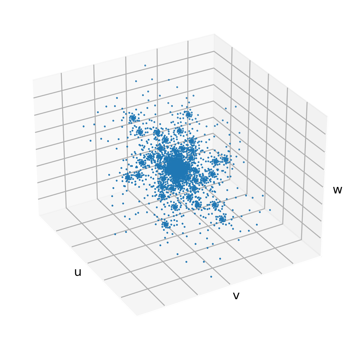
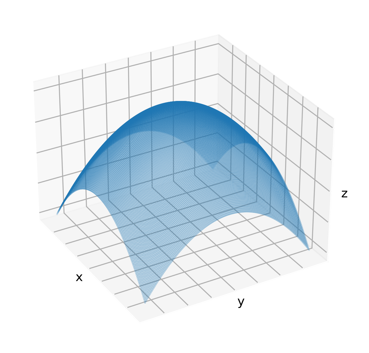
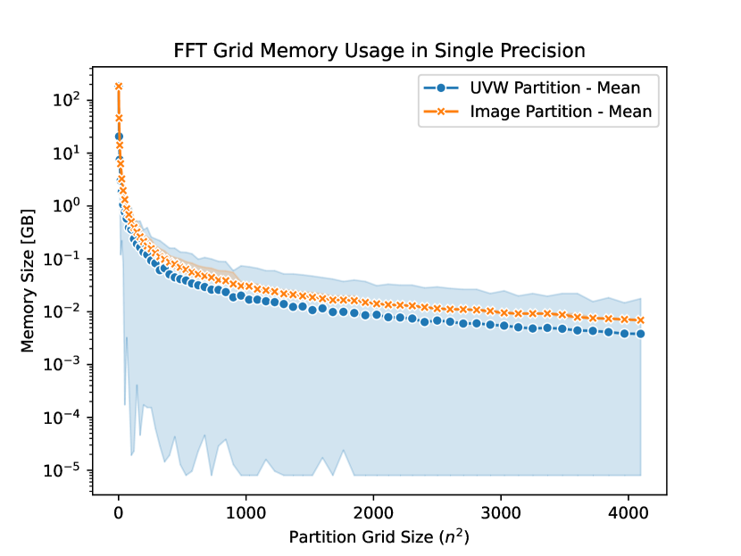
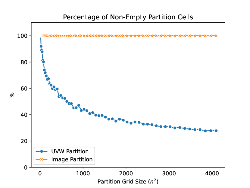
We implemented domain partitioning using a regular 3D grid for both input and output. Figure 1 shows the results for simulated SKA-Low data with partitioning of the input UVW domain and output image domain. The input data consists of clustered points with some individually scattered around the domain, while output points are evenly spaced on a curved surface.

In Figure 1(c), the memory usage per FFT is shown using a partitioning grid of size $(n,n,1)$. For output partitioning of the more evenly spaced points, there is barely any difference in FFT grid size between each domain cell. In contrast, there is a wide variability in FFT grid size for the input UVW partitioning. This is also reflected in Figure 1(d), which shows the percentage of domain cells containing any data points. For large partition grid sizes, as little as 30% of the domain cells require the computation of a NUFFT, which may, therefore, reduce the total number of operations required. However, a NUFFT will also require the spreading of input data and interpolation to output data, which only partially benefit from a smaller FFT grid size.

Whether domain partitioning provides a performance benefit is, therefore, highly dependent on the input and output distribution. It does, however, provide an avenue for parallelization and, as shown in Figure 1(c), can reduce memory usage from over 200 GB to less than 1 GB.

3.5 Discussion

The Bluebild algorithm does not include any additional regularization terms. As such, the images produced by BIPP are comparable to the “dirty” images produced by standard radio astronomy imaging algorithms, i. e. the true image of the sky is convolved with the instrument’s point spread function (Taylor et al., 1999). Additional deconvolution is required to produce a comparable “clean” image. Nevertheless, the eigenvalue decomposition offers some interesting advantages, as discussed in Section 6.

Currently, BIPP does not support image weighting. Output images are equivalent to “natural weighting”, causing scales that have more baselines to dominate the image. Without reweighting, the system noise has the smallest effect on the image, but resolution and sidelobe noise are worse.

BIPP reconstructs the image, including all baselines, even if those baselines provide a resolution higher than the imaging resolution. In other radio astronomical imaging libraries, these longer baselines are discarded to improve performance. The effect of baseline truncation must be kept in mind when comparing BIPP to other imaging software.

Finally, while BIPP has been extensively validated against MS files from MWA and LOFAR, as discussed in Section 4, we have not exhaustively tested MS input files from every telescope. BIPP reads in time-varying antenna and station positions, which are not necessarily structured the same in CASA MeasurementSet files from different telescopes.

4 Validation

To validate our implementation of Bluebild, we compare the outputs of BIPP with the outputs of the original Python implementation. Furthermore, we compare the consistency of our implementations of Standard Synthesis with NUFFT synthesis and the CPU and GPU implementations. In total, we compare five different implementations of the Bluebild algorithm:

• BluebildSsCpu: Original implementation in Python of the Standard Synthesis algorithm from the pypeline library (Kashani, 2017), running on CPU

• BippSsCpu: C++ implementation of the Standard Synthesis algorithm, running on CPU

• BippSsGpu: C++ implementation of the Standard Synthesis algorithm, running on GPU

• BippNufftCpu: C++ implementation of the NUFFT Synthesis algorithm, running on CPU

• BippNufftGpu: C++ implementation of the NUFFT Synthesis algorithm, running on GPU

For the validation tests, the NUFFT user-requested tolerance $\epsilon$ was set to $10^{-5}$.

Furthermore, we compare the BIPP output images to those produced with two reference packages in the field: WSClean (version 3.2) (Offringa et al., 2014) and the tclean task from CASA (version 6.5.3) (McMullin et al., 2007). For both of these imaging libraries, the number of cleaning iterations is set to zero. Thus, we only compare dirty images to BIPP outputs.

4.1 Dataset

For our validation checks, we use OSKAR (Mort et al. (2010), release 2.8.3) to create four simulated SKA-Low telescope observations with a configuration of 512 stations and variable field-of-view (FoV) of 17, 34, 68 or 136 arcmin. We create a radio sky with 9 point sources of 1 Jy spread over a regular grid over the FoV. 50 time steps were generated spread over an observing period of 6 hours.

The simulated visibility data are then processed with CASA, WSClean and all five implementations of Bluebild. In all cases, no cleaning was performed, and Bluebild LSQ images $\widetilde{I}$ are compared to the CASA and WSClean so-called "dirty" images. To ensure a fair comparison, the resolution was fixed to 4 arcsec, so to prevent the visibility truncation of WSClean and CASA as discussed in Section 3.5. This results in square images with $256^{2}$, $512^{2}$, $1024^{2}$ and $2048^{2}$ pixels.

These same datasets and imaging strategies are used for the performance benchmarks described in Section 5.

4.2 Impact of the energy clustering

For each of the five implementations of Bluebild we assess the impact of the energy level clustering (see Sect. 2.4) on image reconstruction. All eigenvalues (positive and negative) are considered, with no eigenvalue truncations, such that $N_{\text{eig}}=L$. Eigenvectors $\alpha_{a}$ with positive eigenvalues are clustered into 1, 2, 4, or 8 distinct energy levels, and all eigenvectors with negative eigenvalues are clustered into a single separate layer. The resulting LSQ-filtered energy levels $\widetilde{I}_{i}$ are summed together to create the complete LSQ image $\widetilde{I}$.

Solution	Im. size	Levels	Maximal range	RMS
	[pixel]		[Jy/beam]	[Jy/beam]
BluebildSsCpu	256	1 & 4	[-5.36e-7, 4.17e-7]	8.93e-8
BippSsGpu	2048	1 & 8	[-1.61e-6, 7.75e-7]	2.09e-8
BippSsCpu	2048	1 & 8	[-1.85e-6, 6.56e-7]	2.10e-8
BippNufftGpu	256	1 & 4	[-1.26e-4, 1.43e-4]	2.80e-5
BippNufftCpu	256	1 & 8	[-2.03e-6, 2.50e-6]	6.41e-7

Table 1: Maximal range of intensity differences reported for each implementation of Bluebild when comparing images obtained using different number of energy levels for the clustering of the eigenvalues.

For each implementation and each image size we assess the impact of the energy clustering by computing differences between images. Results are summarized in Table 1, which gathers, for each solution, the largest interval of differences between two energy levels overall image sizes. We emphasize here that Table 1 reports the worst-case scenarios for each implementation. We find that the energy clustering scheme has a negligible impact on the resulting image, as expected from Eq. 28. The errors observed are consistent with single-point floating precision used in the calculation for Standard Synthesis implementations and consistent with the tolerance $\epsilon=10^{-5}$ tolerance for NUFFT implementations, as expected.

4.3 Consistency between implementations

Figure 2: Inter-solution consistency between the different implementations of Bluebild for images of 1024 x 1024 pixels and produced using a single positive energy layer. Similar results are obtained when using 2, 4 or 8 positive energy levels, see Section 2.4. For completeness, similar plots for image sizes 256, 512 and 2048 are provided in Appendix 9.

Figure 3: Top plot: recovered intensities given in percentage of the simulated intensity (1 Jy point sources) and bottom plot: distance between the recovered source positions and the simulated ones, in pixels, all plotted against the distance in pixels to the centre of the field of view. A recovery superior to 100% indicates an overestimation of the simulated source, and vice versa. The BIPP solution (in red) was obtained with BIPP NUFFT GPU (BippNufftGpu) implementation for an image of $2048\times 2048$ pixels.

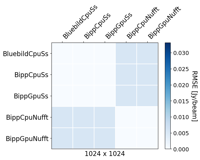
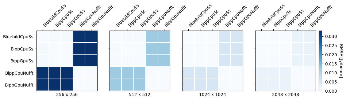
We evaluate the consistency of the images produced by our five implementations of Bluebild. Consistency here is measured as the RMS of pixel intensity differences between two images, referred to as the RMS error or RMSE. Figure 2 presents the inter-solution consistency for the $1024^{2}$ pixel image. For completeness, similar plots for the remaining image sizes ($256^{2}$, $512^{2}$ and $2048^{2}$ pixels) are provided in Appendix 9.

We observe excellent agreement between all Standard Synthesis images and excellent agreement between the two NUFFT Synthesis images. However, there is a percent-level disagreement between the Standard Synthesis and NUFFT Synthesis implementations. In Figures 4(a) and 4(b) for the $2048^{2}$ pixel images it appears that Standard Synthesis slightly underestimates fluxes compared to NUFFT Synthesis over the entire field of view. As the agreement between the NUFFT solution and WSClean and CASA is excellent, this indicates that our implementation of Standard Synthesis underestimates flux values in reconstruction.

Standard Synthesis and NUFFT synthesis should produce equivalent LSQ images $\widetilde{I}$. The principle difference between these algorithms is the treatment of the sampling operator. NUFFT synthesis uses the $uvw$ coordinates directly read from an observation file, in the same way as WSClean or CASA. Standard Synthesis must calculate the instantaneous antenna positions. To do this, it uses the instrument geometry, the observation time, and the coordinate transform operations from astropy (Astropy Collaboration et al., 2013, 2018, 2022). This may introduce additional offset errors compared to the other methods. Due to this, we recommend that users of BIPP use the NUFFT Synthesis implementation.

4.4 Recovering simulated point sources

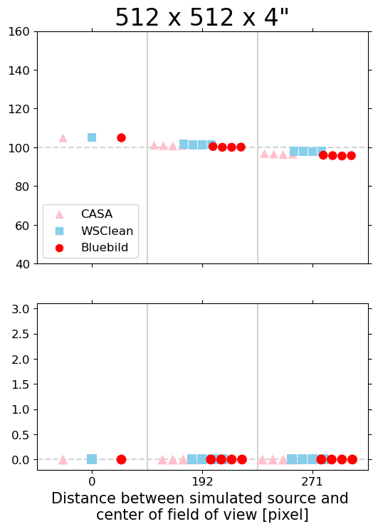
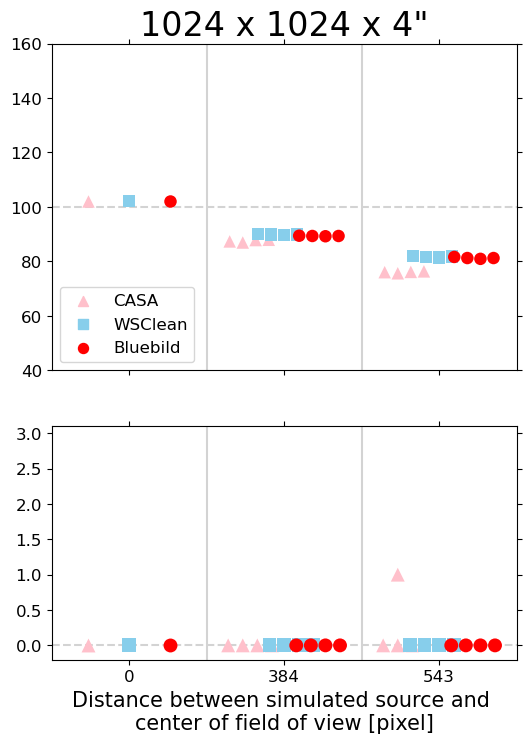
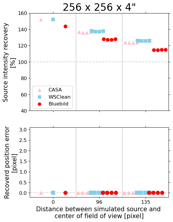
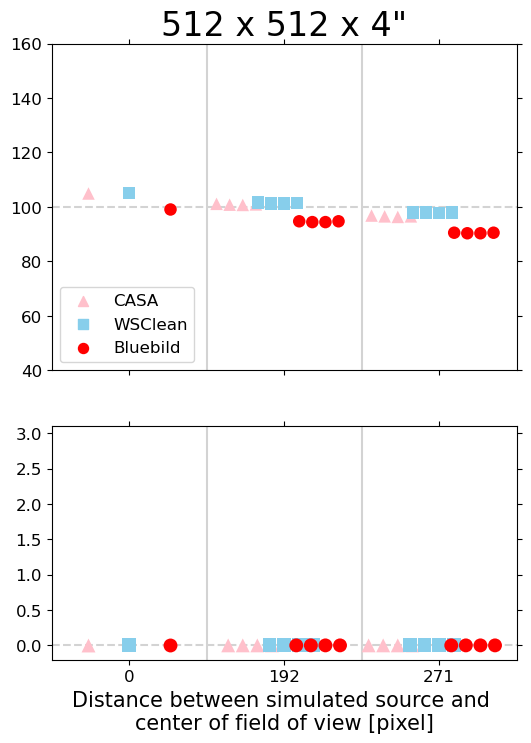
In addition to checking the per-pixel consistency between imaging solutions, we also evaluate the ability of the three packages CASA, WSClean, and BIPP to recover properties of the simulated point sources in our validation dataset. We calculate:

1. The distance (in pixels) between recovered and simulated sources’ positions.

2. The intensity of the recovered sources compared to the simulated ones (1 Jy everywhere).

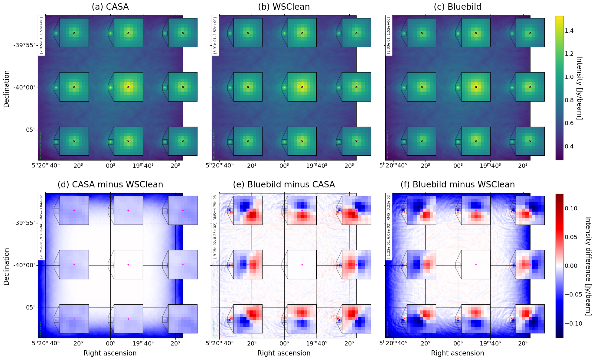
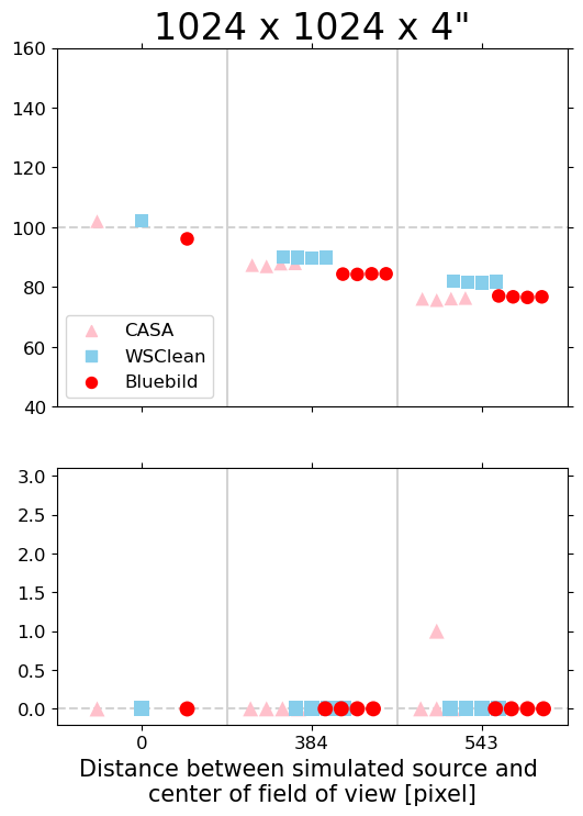
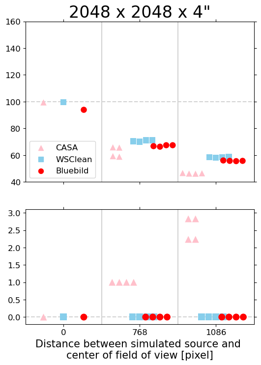
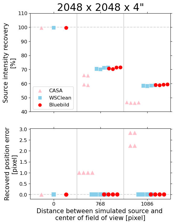
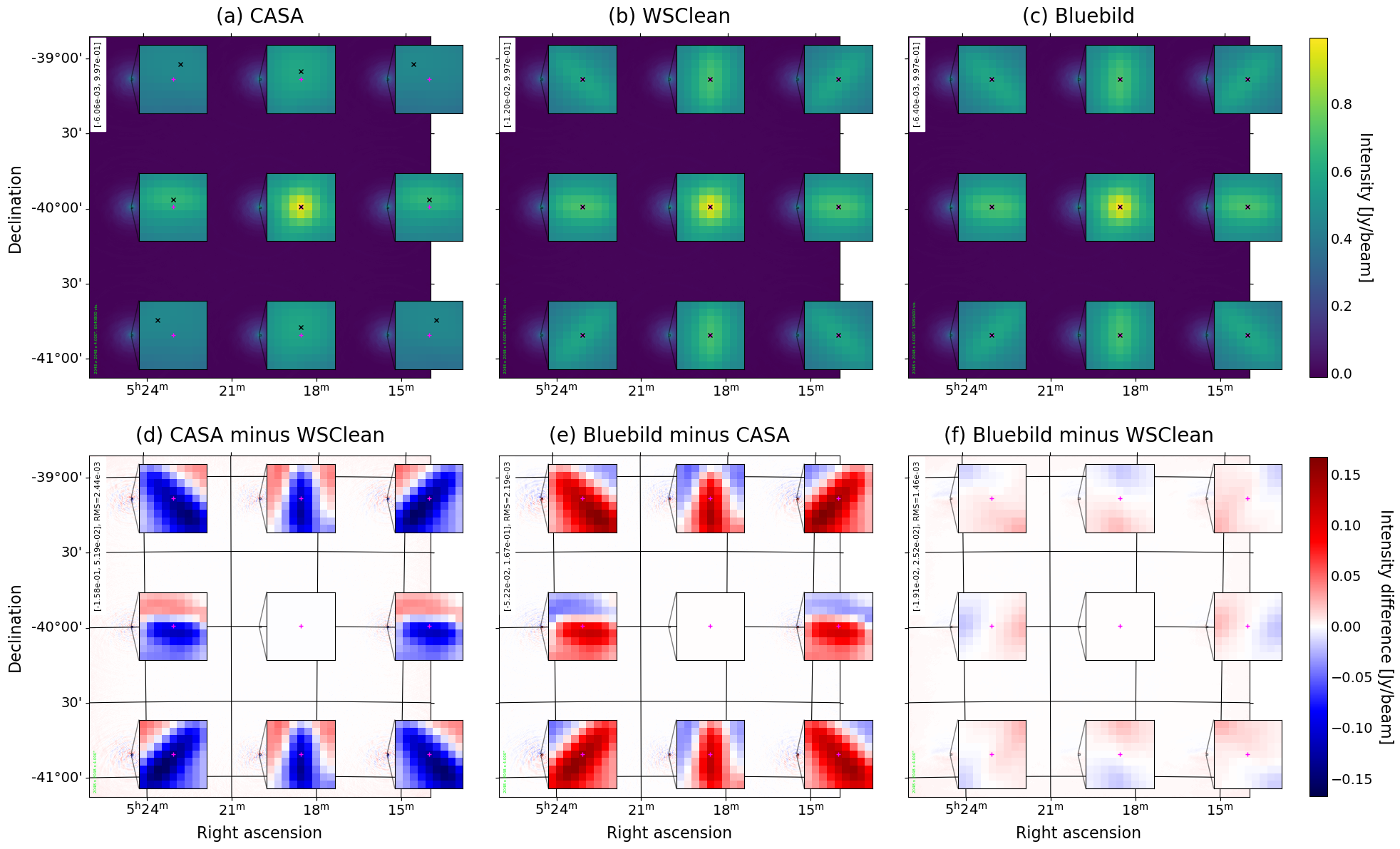
In Figure 4 we show the outputs of CASA, WSClean, and BIPP imaging the same visiblities to create $2048^{2}$ images with 4" resolution. Pink crosses indicate the true/simulated positions of the point sources, and dark crosses indicate their recovered positions, taken as the position of the pixel of highest intensity in the vicinity of the location of the simulated source ($9\times 9$ pixels square area centred on the source’s true location).

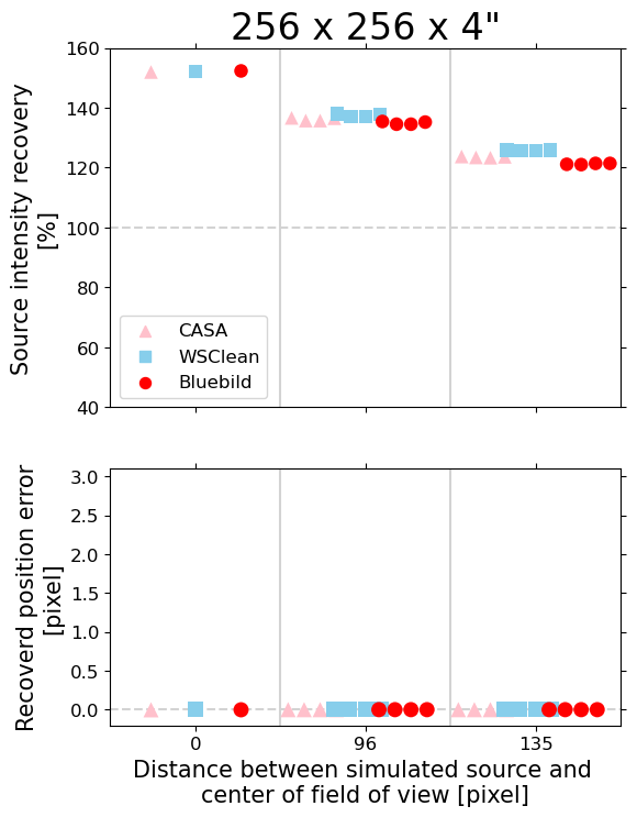
Figure 3 provides a summary of the recovery of the point sources for the BippNufftGpu solution for an image of $2048^{2}$ pixels. The results for all image sizes for the solutions of solutions BippNufftGpu and BippSsCpu are provided in Appendix 9. With an image size $\geq 1024^{2}$ pixels, all three software packages are very similar in the reconstruction of the simulated sky, nicely recovering the position and intensity of the central source. However, for the largest image size with FoV = 32 arcmins, CASA starts to exhibit worse performance compared to WSClean and BIPP, which stay very consistent and able to recover the simulated positions perfectly. This is likely due to the lack of a w-term correction in the default CASA imaging call.

Overall, BIPP is on par with WSClean when it comes to recovering simulated point sources, as shown by the bottom right plot in Figure 4(a). The difference between their two images ranges between -0.019 and +0.026 Jy/beam whereas between CASA and WSClean the difference ranges from -0.157 and +0.052 Jy/beam. The RMS differences also reflect the overall better agreement between Bluebild and WSClean than between CASA and WSClean, with RMS of $1.46\times 10^{-3}$ Jy/beam compared to $2.44\times 10^{-3}$ Jy/beam, respectively.

(a) Using BIPP NUFFT Synthesis GPU (BippNufftGpu)

(b) Using BIPP Standard Synthesis CPU (BippSsCpu)

Figure 4: Recovered simulated 1 Jy point sources by CASA, WSClean and BIPP and differences between output images. Images are of $2048\times 2048\times 4$" resolution. Pink crosses indicate the positions of the simulated sources whereas the black ones indicate the position of recovered sources, i.e. the position of pixel of highest intensity in the vicinity of the true position. On the top part of the figure, the BIPP solution was obtained with the NUFFT Synthesis algorithm and running on GPU, whereas on the bottom part of the figure, the BIPP solution was obtained with the Standard Synthesis algorithm running on CPU.

4.5 Processing real LOFAR data

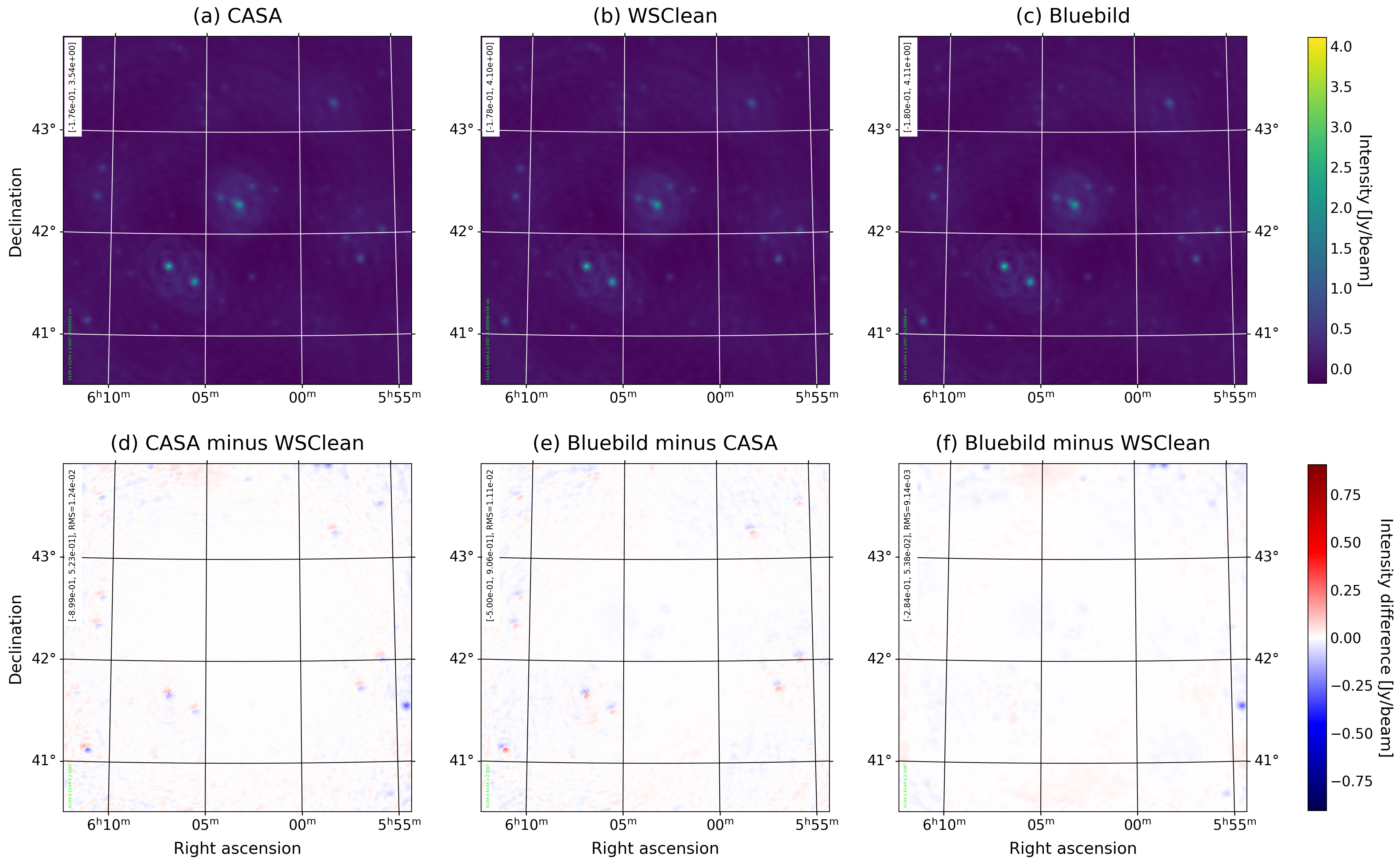
Finally, we also check the output of BIPP on real data collected by the Low-Frequency Array (LOFAR) telescope. We use dataset IV from Pan et al. (2017), a LOFAR observation of the “Toothbrush” cluster RX J0603.3+4214 from 36 stations over the period 2013-02-24-15:32:01.42 to 2013-02-25-00:09:24.51, resulting into 3,123 observation epochs. Dirty images of $6144\times 6144$ pixels of 2" angular resolution were computed with CASA and WSClean, and compared to the LSQ image $\widetilde{I}$ produced by BIPP. The BIPP solution was obtained with the BippNufftGpu implementation with a convergence criterion of $\epsilon=10^{-5}$.

The results are shown in Figure 5. The overall similarity between the three solutions is excellent. We observe that (i) CASA and WSClean slightly disagree on the recovered source locations as indicated by the positive and negative regions (red and blue lobes in subplot (d) of Fig. 5) around sources’ locations, (ii) BIPP and WSClean perfectly agree in recovered sources’ positions and intensities, and (iii) WSClean seems to detect a light source at around (5h54m, 41.5^∘) that does not show up in CASA and BIPP output images. Apart from that, the dirty images from WSClean the LSQ images from BIPP are in remarkable agreement.

Figure 5: Top row: dirty maps produced with (a) CASA, (b) WSClean, (c) BIPP using real LOFAR data from the Toothbrush cluster RX J0603.3+4214 dataset from Pan et al. (2017). Images produced are 6144 by 6144 pixels of $2"$ angular resolution. Bottom row: differences between the following pairs of dirty maps: (d) CASA minus WSClean, (e) BIPP minus CASA and (f) BIPP minus WSClean.

5 Performance Tests

In this section we examine the computational performance of the five implementations of the Bluebild algorithm (i.e. BluebildSsCpu, BippSsCpu, BippSsGpu, BippNufftCpu and BippNufftCpu as described in Section 4) to the reference packages CASA and WSClean. As in Section 4, we only compare the execution time for CASA and WSClean to create dirty images.

For the benchmark, we use the same sets of data as described in Section 4.1. We process 50 epochs of OSKAR simulated SKA-Low observations based on 512 observing stations. The pixel angular resolution was fixed to 4 arcsec while the size of the image was set to either $256^{2}$, $512^{2}$, $1024^{2}$ or $2048^{2}$ pixels, resulting in a varying FoV. For each of these image sizes, all five Bluebild implementations were run with 1, 2, 4 and 8 positive energy levels on top of a single negative energy level containing all of the negative eigenvalues. So, in total, our benchmark contains, for each image size, $4\times 5=20$ Bluebild results.

All the computations were carried out using single-precision (32-bits) floating-point numbers. NUFFT partitioning for both uvw and image domains was set to (4, 4, 1), as described in Section 1. The code was compiled using the GCC v11.3.0 and NVCC v11.8.89 compilers.

Each solution is run with exclusive access to one of the large memory nodes of the GPU cluster of EPFL called Izar. Each node has 384 GB of DDR4 RAM, 2 Intel Xeon Gold 6230 CPUs running at 2.10 GHz with 20 physical cores each (one thread per physical core), and 2 NVidia V100 PCIe 32 GB GPUs. Multi-threaded regions of the code use the 40 CPU cores available. GPU-accelerated parts of the code use a single GPU out of the two available.

5.1 Times to solutions and speedup factors

Figure 6: Top row: times to solutions for 1 energy level (left) and 8 energy levels (right). Bottom row: corresponding speedup factors computed over the reference BluebildSsCpu solution.

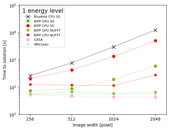
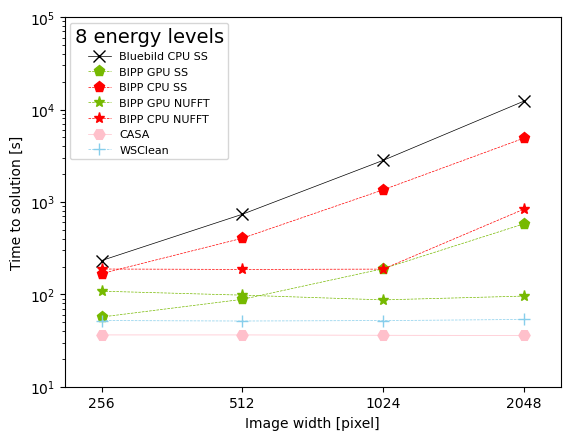
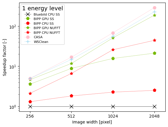
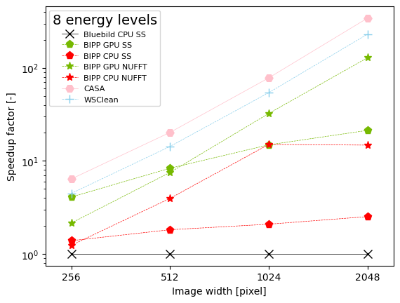
We analyse the times to solutions (TTS) and speedup factors (SF) obtained with the different BIPP implementations when compared to the reference Python implementation of Bluebild. Results are displayed in Figure 6 for 1 energy level (left) and 8 energy levels (right).

Figure 6 clearly highlights the superiority of NUFFT Synthesis compared to the Standard Synthesis. Furthermore, the NUFFT GPU implementation outperforms its CPU counterpart. Table 2 provides the speedup factors of all BIPP solutions, CASA and WSClean when compared to Bluebild in producing images. We see that lower resolutions and a single energy level, BippNufftGpu performs on a similar level than WSClean, or slightly better, but CASA remains the fastest imaging library.

The creation of multiple energy levels with BIPP impacts the performances of the NUFFT-based implementations, but only by adding a constant multiplicative factor. This is expected, as imaging with $N$ energy levels results in at least $N$ calls to the NUFFT operation.

Solution	Speedup factors [-]
	1 energy level					8 energy levels
Image size	$256^{2}$	$512^{2}$	$1024^{2}$	$2048^{2}$		$256^{2}$	$512^{2}$	$1024^{2}$	$2048^{2}$
FoV [arcmin]	17	34	68	136		17	34	68	136
BippSsCpu	1.58	2.10	2.44	3.01		1.55	2.12	2.43	2.82
BippSsGpu	4.69	8.58	18.47	28.78		4.81	8.74	18.18	28.94
BippNufftCpu	1.98	5.91	23.92	100.97		1.19	3.49	13.05	55.23
BippNufftGpu	5.05	15.05	57.77	196.47		3.39	11.13	38.73	159.69
CASA	7.66	24.21	89.40	363.32		7.53	24.42	91.01	373.38
WSClean	4.37	13.83	53.14	228.31		4.26	14.04	53.11	223.59

Table 2: Speedup factors for BIPP, CASA and WSClean solutions compared to the reference Bluebild Python implementation to produce images with 256, 512, 1024 and 2048 pixels resolutions. BIPP speedups in the left part of the table were obtained, setting up 1 positive energy level, while on the right-hand side are given the speedup factors obtained when setting up 8 positive energy levels. The small differences observed for CASA and WSClean results between the 1 and 8 energy levels setups stem from instabilities inherent to using shared resources (CASA and WSClean were run by default along each solution).

5.2 Possible improvements

Process	TTS [s]	% Total
Total	57.72	100%
Reading visibilities (Parameter Estimation)	17.0	29.5 %
Reading visibilities (Imaging)	15.9	27.6 %
Imaging	14.4	25.0 %
Parameter Estimation	4.1	7.1 %
Plotting	2.0	3.5 %
Other	4.2	7.2 %

Table 3: Decomposition of the times to solution (TTS) for the BIPP NUFFT GPU solution obtained with a single positive energy level when generating a 1024 x 1024 pixel image. Parameter Estimation and Imaging are the two main processing blocks of a standard imaging pipeline with BIPP, but we separately time the process to read the visibilities from a MS dataset and pre-process them.

Table 3 presents the decomposition of the time to solutions for the best performing BIPP solution, namely the BIPP NUFFT GPU implementation when constructing the LSQ image using only a single energy level. Performance-wise, this solution is almost on par with WSClean (see left column of Fig. 6).

A striking point from Table 3 is the significant amount of time spent by BIPP on reading and pre-processing the visibilities from the MS input files. Ongoing work is aiming to reduce that time by an order of magnitude. Currently, approximately 33 s of the total 58 s TTS is spent on reading input files. Reducing this operation to about 4 s would lower the TTS down to 29 s, resulting in a better TTS for BIPP over WSClean (55 s) and CASA (35 s).

6 Scientific Applications

One of the unique aspects of BIPP compared to other imagers is that the sky is reconstructed in distinct orthonormal eigenimages:

$$\widetilde{I}=\sum_{a}\lambda_{a}|\epsilon_{a}|^{2}=\sum_{a}\lambda_{a}|\Psi\alpha_{a}|^{2}~{}.$$ (28)

The eigenimages $|\epsilon_{a}|^{2}$ can be reconstructed from each visibility eigenvector $\alpha_{a}$ in parallel. These eigenimages and eigenvisibilities can be sorted and clustered by their eigenvalues $\lambda_{a}$, allowing for natural separation of radio sources in the sky based on their intensity.

For example, for a model field consisting of many point sources which are imaged into three levels using k-means clustering, we are likely to find the brightest intensity sources in the first combined energy level, the intermediate intensity sources in the second energy level and the weakest intensity sources as well as noise in the last energy level. This source separation is a unique benefit of the algorithm, and we present a few examples of this energy separation. These examples make use of BIPP’s inbuilt k-means clustering to combine different eigenimages into distinct energy levels.

6.1 Point sources

Figure 7: Simulated data of the MWA-GLEAM catalogue and decomposition into four energy levels with BIPP. The top-left Figure shows the least-squared image of the combined eigenvectors, producing the LSQ image. The eigenvectors are separated into five energy levels based on their intensity, shown in order of decreasing intensity from left to right, top to bottom.

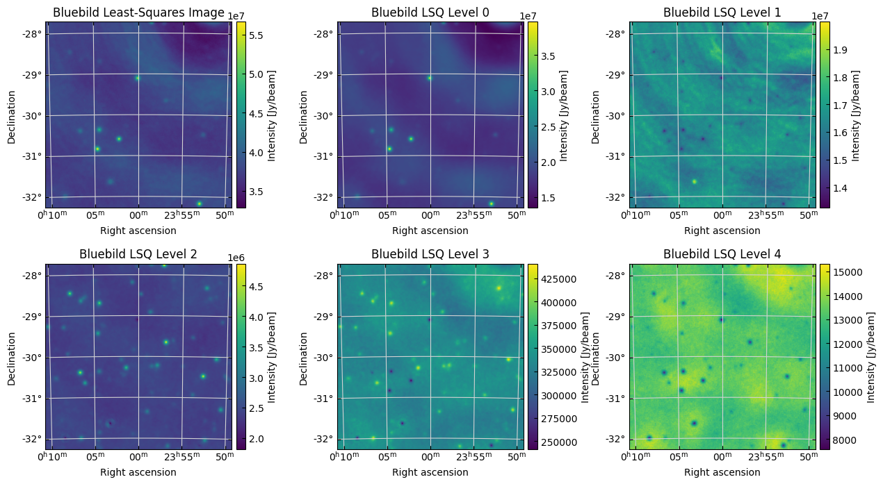
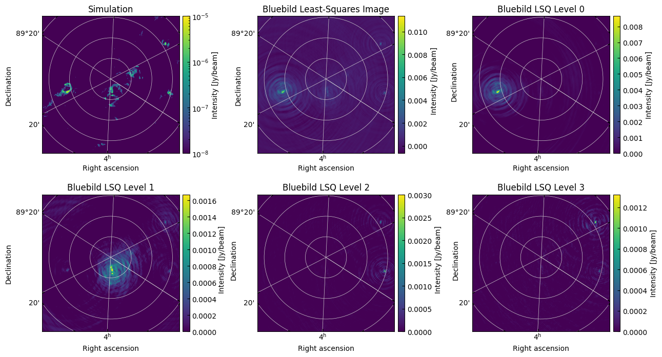
In Figure 7, we show an example of the point source separation performed by BIPP on simulated data of the GaLactic and Extragalactic All-sky MWA Survey (GLEAM) catalogue (Hurley-Walker et al., 2017). We simulate the visibilities with the OSKAR code (Mort et al., 2010) for a field of view (FoV) of $4.55\,\rm deg$, image pixel size of $N_{\rm pix}=1024^{2}$, pointing at $({\rm RA},{\rm Dec})=(0{\rm h},\,-30\,{\rm deg})$ for the SKA-Low layout. The integrated flux of the point sources has been normalised for frequency depth of $\Delta\nu=100\,{\rm kHz}$ and scaled for an observed frequency of $\nu_{\rm obs}=181\,{\rm MHz}$.

Within BIPP we perform eigenvalue truncation, using only the $N_{\text{eig}}$ leading eigenvisibilities $\alpha_{a}$, where the $N_{\text{eig}}$ leading eigenvisibilities correspond to 95% of the total energy of the LSQ image. The remaining eigenvisibilities are partitioned into five distinct levels by grouping their eigenvalues $\lambda_{a}$, and used to reconstruct four distinct images.

In the first panel of Figure 7, top-left, we show the combined LSQ image obtained by adding together all five energy levels. This is equivalent to summing all of the distinct eigenimages before clustering or summing all of the eigenvalues before imaging. As shown in Section 4, the combined image is very similar to the dirty image produced by WSClean.

The images corresponding to the five energy levels are shown in the subsequent panels in decreasing order of energy. Level 0, the top-middle panel, collects the brightest sources in the image. In level 1, top-right panel, we can notice that the algorithm picks most of the residual of the synthesised beam from a radio point source located outside of the FoV as well as one source of the same intensity at $({\rm RA},{\rm Dec})=(0{\rm h}3{\rm m}18{\rm s},\,-31.63\,{\rm deg})$. Meanwhile, from levels 1 to 3, we find the sources separated into levels from the highest to the lowest intensity. The last level contains the majority of residual noise from the sources themselves. We note that due to the functional PCA decomposition, in levels 2 and 3, we can discern sources that otherwise would be too faint and, therefore, difficult to detect from the reduced image (top-left) when in the presence of brighter sources. For levels 1 and higher, the images show ’holes’ with low intensity where the brightest sources are located, indicating that their intensity is completely removed from these lower-level images.

For a real scientific use case, one can imagine that higher levels can be removed in order to reduce the contamination from the point-spread function of bright point sources on dimmer point sources.

6.2 Diffuse emission

In Figure 8, we show another example of source separation, but in this case, for diffuse radio emission. Here, we employ the LoSiTo python package (Edler et al., 2021) to produce simulated LOFAR visibilities. As a sky model, we employ an image with $\text{FoV}=1.1\,\rm deg$, pointing at $({\rm RA},\,{\rm Dec})=(3{\rm h}49{\rm m}11{\rm s},\,90\,{\rm deg})$ and with $N_{\rm pix}=2000$ obtained from the LoTTS data release 1 catalogue (Shimwell et al., 2019). In Figure 8 top-left panel, we show the image employed as a sky model in LoSiTo.

As we mention in Section 3.5, BIPP does not yet include image weighting. We pre-process the visibilities by applying a simple radial weight, $W_{i}=\sqrt{u^{2}_{i}+v^{2}_{i}}$ in order to resolve the small-scale structures that we see in the sky model.

We use BIPP to reconstruct the leading $N_{\text{eig}}$ eigenvisibilities in five distinct levels using k-means clustering, where the $N_{\text{eig}}$ leading eigenvisibilities correspond to 95% of the total energy. Similar to the previous case, we show the combined LSQ image as a reference and highlight the advantage of the functional PCA. In this case, we notice that the only visible feature in the LSQ image is the bright emission at $({\rm RA},\,{\rm Dec})=(4{\rm h}24{\rm m}27{\rm s},\,89.59\,{\rm deg})$. The same feature appears in level 0, whereas a more broad but fainter emission, close to the field centre, is now apparent in level 1 thanks to the decomposition. In this example, levels 2 and 3 both contain traces of the two faint sources at $(15{\rm h}13{\rm m}21{\rm s},\,89.56\,{\rm deg})$ and $(18{\rm h}28{\rm m}20{\rm s},\,89.48\,{\rm deg})$ as they have similar intensities. However, level 2 contains the brightest source of the two, thus proving that the energy level clustering performed by BIPP can further help separate point and diffuse sources as far as their emission is of the same intensity.

Figure 8: Simulated data with the LoSiTo code decomposed into four eigen-levels by BIPP functional PCA. The top-left panel shows the sky model employed as input for LoSiTo. The top-centre panel shows the least-squared image of the combined eigenimages, equivalent to a dirty image. From left to right, top to bottom, the four eigenimages are separated into five levels based on the k-means algorithm.

7 Conclusions

We have presented BIPP, an HPC implementation of the Bluebild algorithm. BIPP offers an alternative strategy for interferometric imaging, producing LSQ estimates of the sky, using fPCA to reconstruct the sky in distinct energy levels, and levering the NUFFT for fast image synthesis. We demonstrate the BIPP reconstructs observations with competitive image fidelity compared to the WSClean  $w$-stacking implementation and similar time-to-solution.

Because BIPP can reconstructs images in distinct energy levels, it may offer considerable performance advantages over classical imaging algorithms. For example, dim sources can be reconstructed without performing any iterative “peeling” (Williams et al., 2019). We note that while traditional imaging software must pass their outputs through multiple rounds of iterative cleaning to recover dim sources, with BIPP these sources are immediately visible in the smaller-energy levels, as shown in figures 7 and 8. As the time-to-solution comparisons in Section 5 only compare WSClean  and CASA  dirty images to BIPP output images, we note that considerable performance increases may be offered by BIPP if the WSClean  and CASA  dirty images require thousands of additional iterations of cleaning to prepare them for scientific analysis.

Manipulation of the eigenvectors may also allow for scientific analysis that is not possible with combined images. For example, noise suppression can be obtained by discarding the lowest eigenlevels, and foreground removal can be achieved by discarding the highest eigenlevels. The full advantages that this functional PCA can offer for scientific analysis are a future direction of exploration.

Future HPC developments of BIPP will focus on scalability, node-level parallelism of the NUFFT, and optimizing our GPU implementation of the type-3 nufft for radio astronomy data.

Data Availability

Most of the datasets used in validation are simulated observations generated by open-source libraries as documented in the text. These simulated datasets can be made available upon reasonable request to the authors. The real LOFAR data used for validation are available at DOI:10.5281/zenodo.1042525. The BIPP source code is publically available on GitHub.

Appendix A Additional Validation Results

In this Appendix, we present additional validation results and checks of BIPP, for all four image sizes described in Section 4.

The increasing SS and NUFFT solution consistency with the increasing image size is shown in Figure 9. We observe excellent agreement between all Standard Synthesis images, and excellent agreement between the two NUFFT Synthesis images, at all image sizes. However, there is a %-level disagreement between the Standard Synthesis and NUFFT Synthesis implementations which grows as image size and FoV decrease.

The exact cause of this disagreement, and why it increases with smaller FoV size, is not well understood. Standard Synthesis and NUFFT synthesis should produce equivalent LSQ images $\widetilde{I}$. However, there is an important difference between these algorithms in the treatment of the sampling operator. NUFFT synthesis uses the $uvw$ coordinates directly read from an observation file, in the same way as WSClean or CASA. Standard Synthesis must calculate the instantaneous antenna positions. To do this, it uses the instrument geometry, the observation time, and the coordinate transform operations from astropy (Astropy Collaboration et al., 2013, 2018, 2022). This may introduce additional offset errors compared to the other methods.

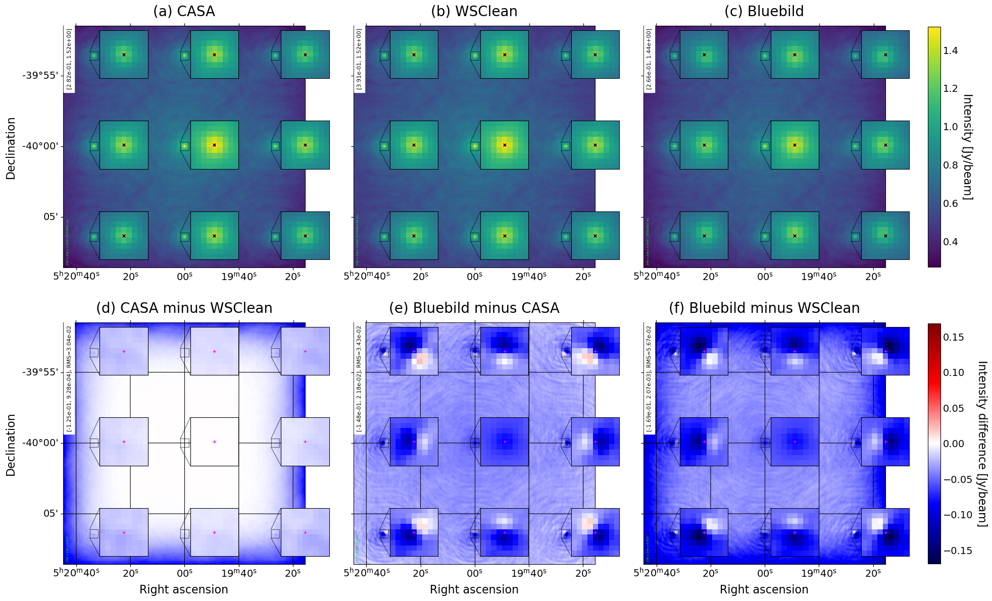
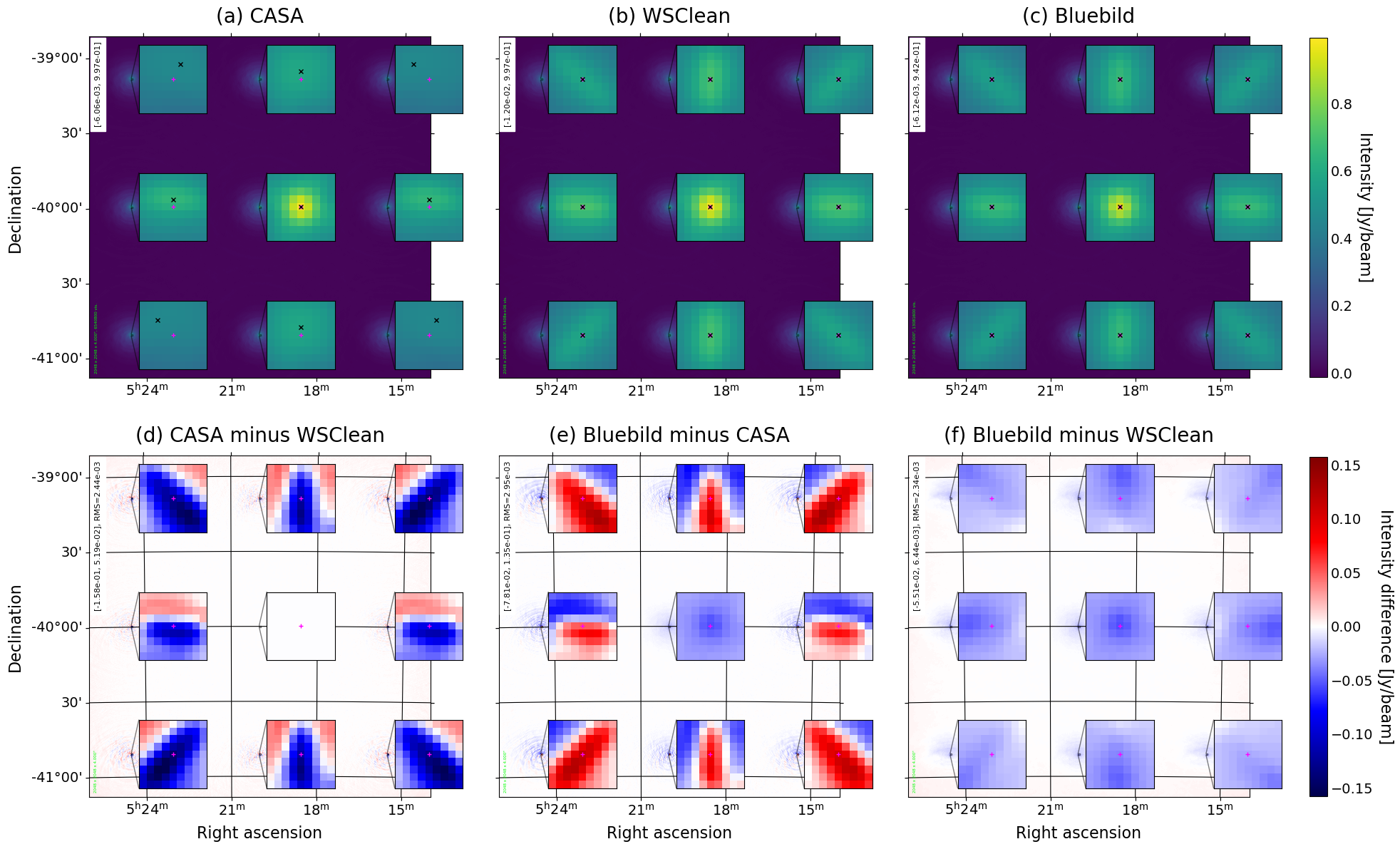
We also compare the output of BIPP , WSClean, and CASA for the small 4.3 arcmin FoV / $256\times 256$ pixel images in Figure 10. This has a FoV divided by 4 compared to Figure 4. The situation is similar, i.e. Standard Synthesis overall underestimates fluxes compared to NUFFT Synthesis and WSClean. We note that this does mean that the Standard Synthesis algorithm is incorrect, as overall, for the smaller FoV images tested here, there is a general overestimation in the recovery of the simulated sources of background noise. For higher resolutions images like Figures 4(a) and 4(b) we see that the range for recovered intensities is comprised between 0.0 and 1.0 Jy/beam, which matches the input of the simulation (1 Jy point sources on a 3 x 3 grid, zero elsewhere). However, if we look at images with lower sizes presented in Figures 10(a) and 10(b), the recovered range of intensity is (a) positively shifted and (b) expanded, resulting in ranges of [2.82e-1, 1.52e0] and [3.91e-1, 1.52e0] for CASA and WSClean, whereas for BIPP Standard Synthesis the range is [2.66e-1, 1.44e-1].

Figure 12 summarizes the point source recovery tests for the three imaging libraries. We see that the Standard Synthesis solution for low-size images is, in fact, closer to the true simulated sky, although for higher resolution, a general underestimation of fluxes by a few per cent is observed. For the smallest FoV and image size, all packages tend to overestimate the intensity of the sources (up to 152.1%), likely due to effects from the point spread function of the instrument. An excellent reconstruction is obtained for images of $512^{2}$ pixels, with only a slight overestimation of the point source located in the centre of FoV and a slight underestimation of the intensity of the 4 point sources the furthest apart from the image centre (at a distance of 271 pixels).

Figure 9: Inter-solution consistency between the different implementations of Bluebild decomposed over image resolution, for images produced considering a single positive energy layer. Similar results are obtained using 2, 4 or 8 positive energy levels.

(a) Using BIPP NUFFT GPU

(b) Using BIPP SS CPU

Figure 10: Recovered simulated 1 Jy point sources by CASA, WSClean and Bluebild and differences between dirty images. Images are of 256 x 256 x 4" resolution. Pink crosses indicate the positions of the simulated sources, whereas the black ones indicate the position of recovered sources, i.e. the position of the pixel of highest intensity in the vicinity of the true position. On the top part of the figure, the BIPP solution was obtained with the NUFFT algorithm and running on GPU, whereas on the bottom part of the figure the BIPP solution was obtained with the SS algorithm running on CPU.

Figure 11: Top plots: recovered intensities given in percentage of the simulated intensity (1 Jy point sources) and bottom plots: distance between the recovered source positions and the simulated ones, in pixels, all plotted against the distance in pixels to the centre of the field of view. The size of the images increases from the left to the right from 256 to 2048 pixels. A recovery superior to 100% indicates an overestimation of the simulated source, and vice versa. The Bluebild solution (in red) was obtained with BIPP NUFFT GPU implementation.

Figure 12: Top plots: recovered intensities given in percentage of the simulated intensity (1 Jy point sources) and bottom plots: distance between the recovered source positions and the simulated ones, in pixels, all plotted against the distance in pixels to the centre of the field of view. The size of the images increases from the left to the right from 256 to 2048 pixels. A recovery superior to 100% indicates an overestimation of the simulated source, and vice versa. The Bluebild solution (in red) was obtained with BIPP SS CPU implementation.

References

- Astropy Collaboration et al. (2013) Astropy Collaboration, Robitaille, T. P., Tollerud, E. J., Greenfield, P., Droettboom, M., Bray, E., Aldcroft, T., Davis, M., Ginsburg, A., Price-Whelan, A. M., Kerzendorf, W. E., Conley, A., Crighton, N., Barbary, K., Muna, D., Ferguson, H., Grollier, F., Parikh, M. M., Nair, P. H., Unther, H. M., Deil, C., Woillez, J., Conseil, S., Kramer, R., Turner, J. E. H., Singer, L., Fox, R., Weaver, B. A., Zabalza, V., Edwards, Z. I., Azalee Bostroem, K., Burke, D. J., Casey, A. R., Crawford, S. M., Dencheva, N., Ely, J., Jenness, T., Labrie, K., Lim, P. L., Pierfederici, F., Pontzen, A., Ptak, A., Refsdal, B., Servillat, M., & Streicher, O., 2013. Astropy: A community Python package for astronomy, A&A, 558, A33.
- Astropy Collaboration et al. (2018) Astropy Collaboration, Price-Whelan, A. M., Sipőcz, B. M., Günther, H. M., Lim, P. L., Crawford, S. M., Conseil, S., Shupe, D. L., Craig, M. W., Dencheva, N., Ginsburg, A., Vand erPlas, J. T., Bradley, L. D., Pérez-Suárez, D., de Val-Borro, M., Aldcroft, T. L., Cruz, K. L., Robitaille, T. P., Tollerud, E. J., Ardelean, C., Babej, T., Bach, Y. P., Bachetti, M., Bakanov, A. V., Bamford, S. P., Barentsen, G., Barmby, P., Baumbach, A., Berry, K. L., Biscani, F., Boquien, M., Bostroem, K. A., Bouma, L. G., Brammer, G. B., Bray, E. M., Breytenbach, H., Buddelmeijer, H., Burke, D. J., Calderone, G., Cano Rodríguez, J. L., Cara, M., Cardoso, J. V. M., Cheedella, S., Copin, Y., Corrales, L., Crichton, D., D’Avella, D., Deil, C., Depagne, É., Dietrich, J. P., Donath, A., Droettboom, M., Earl, N., Erben, T., Fabbro, S., Ferreira, L. A., Finethy, T., Fox, R. T., Garrison, L. H., Gibbons, S. L. J., Goldstein, D. A., Gommers, R., Greco, J. P., Greenfield, P., Groener, A. M., Grollier, F., Hagen, A., Hirst, P., Homeier, D., Horton, A. J., Hosseinzadeh, G., Hu, L., Hunkeler, J. S., Ivezić, Ž., Jain, A., Jenness, T., Kanarek, G., Kendrew, S., Kern, N. S., Kerzendorf, W. E., Khvalko, A., King, J., Kirkby, D., Kulkarni, A. M., Kumar, A., Lee, A., Lenz, D., Littlefair, S. P., Ma, Z., Macleod, D. M., Mastropietro, M., McCully, C., Montagnac, S., Morris, B. M., Mueller, M., Mumford, S. J., Muna, D., Murphy, N. A., Nelson, S., Nguyen, G. H., Ninan, J. P., Nöthe, M., Ogaz, S., Oh, S., Parejko, J. K., Parley, N., Pascual, S., Patil, R., Patil, A. A., Plunkett, A. L., Prochaska, J. X., Rastogi, T., Reddy Janga, V., Sabater, J., Sakurikar, P., Seifert, M., Sherbert, L. E., Sherwood-Taylor, H., Shih, A. Y., Sick, J., Silbiger, M. T., Singanamalla, S., Singer, L. P., Sladen, P. H., Sooley, K. A., Sornarajah, S., Streicher, O., Teuben, P., Thomas, S. W., Tremblay, G. R., Turner, J. E. H., Terrón, V., van Kerkwijk, M. H., de la Vega, A., Watkins, L. L., Weaver, B. A., Whitmore, J. B., Woillez, J., Zabalza, V., & Astropy Contributors, 2018. The Astropy Project: Building an Open-science Project and Status of the v2.0 Core Package, AJ, 156(3), 123.
- Astropy Collaboration et al. (2022) Astropy Collaboration, Price-Whelan, A. M., Lim, P. L., Earl, N., Starkman, N., Bradley, L., Shupe, D. L., Patil, A. A., Corrales, L., Brasseur, C. E., N"othe, M., Donath, A., Tollerud, E., Morris, B. M., Ginsburg, A., Vaher, E., Weaver, B. A., Tocknell, J., Jamieson, W., van Kerkwijk, M. H., Robitaille, T. P., Merry, B., Bachetti, M., G"unther, H. M., Aldcroft, T. L., Alvarado-Montes, J. A., Archibald, A. M., B’odi, A., Bapat, S., Barentsen, G., Baz’an, J., Biswas, M., Boquien, M., Burke, D. J., Cara, D., Cara, M., Conroy, K. E., Conseil, S., Craig, M. W., Cross, R. M., Cruz, K. L., D’Eugenio, F., Dencheva, N., Devillepoix, H. A. R., Dietrich, J. P., Eigenbrot, A. D., Erben, T., Ferreira, L., Foreman-Mackey, D., Fox, R., Freij, N., Garg, S., Geda, R., Glattly, L., Gondhalekar, Y., Gordon, K. D., Grant, D., Greenfield, P., Groener, A. M., Guest, S., Gurovich, S., Handberg, R., Hart, A., Hatfield-Dodds, Z., Homeier, D., Hosseinzadeh, G., Jenness, T., Jones, C. K., Joseph, P., Kalmbach, J. B., Karamehmetoglu, E., Kaluszy’nski, M., Kelley, M. S. P., Kern, N., Kerzendorf, W. E., Koch, E. W., Kulumani, S., Lee, A., Ly, C., Ma, Z., MacBride, C., Maljaars, J. M., Muna, D., Murphy, N. A., Norman, H., O’Steen, R., Oman, K. A., Pacifici, C., Pascual, S., Pascual-Granado, J., Patil, R. R., Perren, G. I., Pickering, T. E., Rastogi, T., Roulston, B. R., Ryan, D. F., Rykoff, E. S., Sabater, J., Sakurikar, P., Salgado, J., Sanghi, A., Saunders, N., Savchenko, V., Schwardt, L., Seifert-Eckert, M., Shih, A. Y., Jain, A. S., Shukla, G., Sick, J., Simpson, C., Singanamalla, S., Singer, L. P., Singhal, J., Sinha, M., SipHocz, B. M., Spitler, L. R., Stansby, D., Streicher, O., Sumak, J., Swinbank, J. D., Taranu, D. S., Tewary, N., Tremblay, G. R., Val-Borro, M. d., Van Kooten, S. J., Vasovi’c, Z., Verma, S., de Miranda Cardoso, J. V., Williams, P. K. G., Wilson, T. J., Winkel, B., Wood-Vasey, W. M., Xue, R., Yoachim, P., Zhang, C., Zonca, A., & Astropy Project Contributors, 2022. The Astropy Project: Sustaining and Growing a Community-oriented Open-source Project and the Latest Major Release (v5.0) of the Core Package, apj, 935(2), 167.
- Bagchi & Mitra (1999) Bagchi, S. & Mitra, S. K., 1999. The Nonuniform Discrete Fourier Transform and Its Applications in Signal Processing, Kluwer Academic Publishers, USA.
- Barnett et al. (2019) Barnett, A. H., Magland, J., & af Klinteberg, L., 2019. A Parallel Nonuniform Fast Fourier Transform Library Based on an “Exponential of Semicircle” Kernel, SIAM Journal on Scientific Computing, 41(5), C479–C504.
- Broekema et al. (2015) Broekema, P. C., van Nieuwpoort, R. V., & Bal, H. E., 2015. The Square Kilometre Array Science Data Processor. Preliminary compute platform design, Journal of Instrumentation, 10(7), C07004.
- Dewdney et al. (2009) Dewdney, P. E., Hall, P. J., Schilizzi, R. T., & Lazio, T. J. L. W., 2009. The Square Kilometre Array, IEEE Proceedings, 97(8), 1482–1496.
- Edler et al. (2021) Edler, H. W., de Gasperin, F., & Rafferty, D., 2021. Investigating ionospheric calibration for LOFAR 2.0 with simulated observations, A&A, 652, A37.
- Frigo & Johnson (1997) Frigo, M. & Johnson, S. G., 1997. The fastest Fourier transform in the west, Tech. Rep. MIT-LCS-TR-728, Massachusetts Institute of Technology.
- Frigo & Johnson (2005) Frigo, M. & Johnson, S. G., 2005. The design and implementation of FFTW3, Proceedings of the IEEE, 93(2), 216–231, Special issue on “Program Generation, Optimization, and Platform Adaptation”.
- Hamaker et al. (1996) Hamaker, J. P., Bregman, J. D., & Sault, R. J., 1996. Understanding radio polarimetry. I. Mathematical foundations., A&AS, 117, 137–147.
- Högbom (1974) Högbom, J. A., 1974. Aperture Synthesis with a Non-Regular Distribution of Interferometer Baselines, A&AS, 15, 417.
- Hurley-Walker et al. (2017) Hurley-Walker, N., Callingham, J. R., Hancock, P. J., Franzen, T. M. O., Hindson, L., Kapińska, A. D., Morgan, J., Offringa, A. R., Wayth, R. B., Wu, C., Zheng, Q., Murphy, T., Bell, M. E., Dwarakanath, K. S., For, B., Gaensler, B. M., Johnston-Hollitt, M., Lenc, E., Procopio, P., Staveley-Smith, L., Ekers, R., Bowman, J. D., Briggs, F., Cappallo, R. J., Deshpande, A. A., Greenhill, L., Hazelton, B. J., Kaplan, D. L., Lonsdale, C. J., McWhirter, S. R., Mitchell, D. A., Morales, M. F., Morgan, E., Oberoi, D., Ord, S. M., Prabu, T., Shankar, N. U., Srivani, K. S., Subrahmanyan, R., Tingay, S. J., Webster, R. L., Williams, A., & Williams, C. L., 2017. GaLactic and Extragalactic All-sky Murchison Widefield Array (GLEAM) survey - I. A low-frequency extragalactic catalogue, MNRAS, 464(1), 1146–1167.
- Kashani (2017) Kashani, S., 2017. Towards real-time high-resolution interferometric imaging with bluebild.
- Kashani et al. (2023) Kashani, S., Rué Queralt, J., Jarret, A., & Simeoni, M., 2023. HVOX: Scalable Interferometric Synthesis and Analysis of Spherical Sky Maps, arXiv e-prints, p. arXiv:2306.06007.
- Lee & Greengard (2005) Lee, J.-Y. & Greengard, L., 2005. The type 3 nonuniform fft and its applications, Journal of Computational Physics, 206(1), 1–5.
- Matthieu Simeoni (In preparation) Matthieu Simeoni, Paul Hurley, S. K., In preparation. Bluebild: Consistent functional principal component imaging for radio astronomy.
- McMullin et al. (2007) McMullin, J. P., Waters, B., Schiebel, D., Young, W., & Golap, K., 2007. CASA Architecture and Applications, in Astronomical Data Analysis Software and Systems XVI, vol. 376 of Astronomical Society of the Pacific Conference Series, p. 127.
- Mort et al. (2010) Mort, B. J., Dulwich, F., Salvini, S., Adami, K. Z., & Jones, M. E., 2010. Oskar: Simulating digital beamforming for the ska aperture array, in 2010 IEEE International Symposium on Phased Array Systems and Technology, pp. 690–694.
- Offringa et al. (2014) Offringa, A. R., McKinley, B., Hurley-Walker, et al., 2014. WSClean: an implementation of a fast, generic wide-field imager for radio astronomy, MNRAS, 444(1), 606–619.
- Pan et al. (2017) Pan, H., Simeoni, M., Hurley, P., Blu, T., & Vetterli, M., 2017. Leap: Looking beyond pixels with continuous-space estimation of point sources, Astronomy & Astrophysics, 608.
- Pence et al. (2010) Pence, W. D., Chiappetti, L., Page, C. G., Shaw, R. A., & Stobie, E., 2010. Definition of the Flexible Image Transport System (FITS), version 3.0, A&A, 524, A42.
- Rau et al. (2009) Rau, U., Bhatnagar, S., Voronkov, M. A., & Cornwell, T. J., 2009. Advances in calibration and imaging techniques in radio interferometry, Proceedings of the IEEE, 97(8), 1472–1481.
- Shih et al. (2021) Shih, Y., Wright, G., Anden, J., Blaschke, J., & Barnett, A. H., 2021. cufinufft: a load-balanced gpu library for general-purpose nonuniform ffts, in 2021 IEEE International Parallel and Distributed Processing Symposium Workshops (IPDPSW), pp. 688–697, IEEE Computer Society, Los Alamitos, CA, USA.
- Shimwell et al. (2019) Shimwell, T. W., Tasse, C., Hardcastle, M. J., Mechev, A. P., Williams, W. L., Best, P. N., Rottgering, H. J. A., Callingham, J. R., Dijkema, T. J., de Gasperin, F., Hoang, D. N., Hugo, B., Mirmont, M., Oonk, J. B. R., Prandoni, I., Rafferty, D., Sabater, J., Smirnov, O., van Weeren, R. J., White, G. J., Atemkeng, M., Bester, L., Bonnassieux, E., Bruggen, M., Brunetti, G., Chyzy, K. T., Cochrane, R., Conway, J. E., Croston, J. H., Danezi, A., Duncan, K., Haverkorn, M., Heald, G. H., Iacobelli, M., Intema, H. T., Jackson, N., Jamrozy, M., Jarvis, M. J., Lakhoo, R., Mevius, M., Miley, G. K., Morabito, L., Morganti, R., Nisbet, D., Orru, E., Perkins, S., Pizzo, R. F., Schrijvers, C., Smith, D. J. B., Vermeulen, R., Wise, M. W., Alegre, L., Bacon, D. J., van Bemmel, I. M., Beswick, R. J., Bonafede, A., Botteon, A., Bourke, S., Brienza, M., Calistro Rivera, G., Cassano, R., Clarke, A. O., Conselice, C. J., Dettmar, R. J., Drabent, A., Dumba, C., Emig, K. L., Ensslin, T. A., Ferrari, C., Garrett, M. A., Genova-Santos, R. T., Goyal, A., Gurkan, G., Hale, C., Harwood, J. J., Heesen, V., Hoeft, M., Orellou, C. H., Jackson, C., Kokotanekov, G., Kondapally, R., Kunert-Bajraszewska, M., Mahatma, V., Mahony, E. K., Mandal, S., McKean, J. P., Merloni, A., Mingo, B., Miskolczi, A., Mooney, S., Nikiel-Wroczynski, B., O’Sullivan, S. P., Quinn, J., Reich, W., Roskowinski, C., Rowlinson, A., Savini, F., Saxena, A., Schwarz, D. J., Shulevski, A., Sridhar, S. S., Stacey, H. R., Urquhart, S., van der Wiel, M. H. D., Varenius, E., Webster, B., & Wilber, A., 2019. VizieR Online Data Catalog: LOFAR Two-metre Sky Survey DR1 source catalog (Shimwell+, 2019), VizieR Online Data Catalog, pp. J/A+A/622/A1.
- Simeoni & Hurley (2019) Simeoni, M. & Hurley, P., 2019. Graph spectral clustering of convolution artefacts in radio interferometric images, in ICASSP 2019 - 2019 IEEE International Conference on Acoustics, Speech and Signal Processing (ICASSP), pp. 4260–4264.
- Smirnov (2011) Smirnov, O. M., 2011. Revisiting the radio interferometer measurement equation. I. A full-sky Jones formalism, A&A, 527, A106.
- Taylor et al. (1999) Taylor, G. B., Carilli, C. L., & Perley, R. A., 1999. Synthesis imaging in radio astronomy ii, in Synthesis Imaging in Radio Astronomy II, vol. 180 of Astronomical Society of the Pacific Conference Series.
- Taylor (1978) Taylor, J. M., 1978. The condition of gram matrices and related problems, Proceedings of the Royal Society of Edinburgh Section A: Mathematics, 80(1-2), 45–56.
- Tomov et al. (2010) Tomov, S., Dongarra, J., & Baboulin, M., 2010. Towards dense linear algebra for hybrid GPU accelerated manycore systems, Parallel Computing, 36(5-6), 232–240.
- van der Veen & Wijnholds (2013) van der Veen, A.-J. & Wijnholds, S. J., 2013. Signal Processing Tools for Radio Astronomy, pp. 421–463, Springer New York, New York, NY.
- Vetterli et al. (2014) Vetterli, M., Kovačević, J., & Goyal, V. K., 2014. Foundations of Signal Processing, Cambridge University Press.
- Williams et al. (2019) Williams, P. K. G., Allers, K. N., Biller, B. A., & Vos, J., 2019. A tool and workflow for radio astronomical “peeling” in casa, Research Notes of the AAS, 3(7), 110.
- Æçal et al. (2015) Æçal, O., Hurley, P., Cherubini, G., & Kazemi, S., 2015. Collaborative randomized beamforming for phased array radio interferometers, in 2015 IEEE International Conference on Acoustics, Speech and Signal Processing (ICASSP), pp. 5654–5658.