Does Graph Distillation See Like Vision Dataset Counterpart?

Abstract

Training on large-scale graphs has achieved remarkable results in graph representation learning, but its cost and storage have attracted increasing concerns. Existing graph condensation methods primarily focus on optimizing the feature matrices of condensed graphs while overlooking the impact of the structure information from the original graphs. To investigate the impact of the structure information, we conduct analysis from the spectral domain and empirically identify substantial Laplacian Energy Distribution (LED) shifts in previous works. Such shifts lead to poor performance in cross-architecture generalization and specific tasks, including anomaly detection and link prediction. In this paper, we propose a novel Structure-broadcasting Graph Dataset Distillation (SGDD) scheme for broadcasting the original structure information to the generation of the synthetic one, which explicitly prevents overlooking the original structure information. Theoretically, the synthetic graphs by SGDD are expected to have smaller LED shifts than previous works, leading to superior performance in both cross-architecture settings and specific tasks. We validate the proposed SGDD across 9 datasets and achieve state-of-the-art results on all of them: for example, on the YelpChi dataset, our approach maintains 98.6% test accuracy of training on the original graph dataset with 1,000 times saving on the scale of the graph. Moreover, we empirically evaluate there exist 17.6% $\sim$ 31.4% reductions in LED shift crossing 9 datasets. Extensive experiments and analysis verify the effectiveness and necessity of the proposed designs. The code is available in the https://github.com/RingBDStack/SGDD.

1 Introduction

Graphs have been applied in many research areas and achieved remarkable results, including social networks [26, 65, 71, 77], physical [15, 3, 55, 10], and chemical interactions [2, 91, 109, 78]. Graph neural networks (GNNs), a classical and wide-studied graph representation learning method [38, 82, 97, 61], is proposed to extract information via modeling the features and structures from the given graph. Nevertheless, the computational and memory costs are extremely heavy when training on a large graph [46, 87, 98, 73]. One of the most straightforward ideas is to reduce the redundancy of the large graph. For example, graph sparsification [64, 75] and coarsening [51, 50, 44] are proposed to achieve this goal by dropping redundant edges and grouping similar nodes. These methods have shown promising results in reducing the size and complexity of large graphs while preserving their essential properties.

However, graph sparsification and coarsening heavily rely on heuristics [5] (e.g., the largest principle eigenvalues [76], pairwise distances [64, 79]), which may lead to poor generalization on various architectures or tasks and sub-optimal for the downstream GNNs training [35]. Most recently, as shown in Fig. 1(a), GCond [35] follows the vision dataset distillation methods [86, 104, 102] and proposes to condense the original graph by the gradient matching strategy. The feature of the synthetic graph dataset is optimized by minimizing the gradient differences between training on original and synthetic graph datasets. Then, the synthetic feature is fed into the function $f(\mathbf{X^{\prime}}$) (e.g., pair-wise feature similarity [72]) to obtain the structure of the graph. The synthetic graph dataset (including feature and structure) is expected to preserve the task-relevant information and achieve comparable results as training on the original graph dataset at an extremely small cost.

(a) Condense scheme of GCond

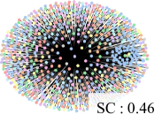
(b) $\mathbf{A^{\prime}}$ of GCond

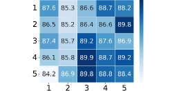
(c) Cross-arch. Acc. of GCond

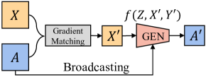
(d) Condense scheme of SGDD

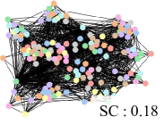
(e) $\mathbf{A^{\prime}}$ of SGDD 

(f) Cross-arch. Acc. of SGDD

Figure 1: (a) and (d) illustrate that the pipelines of SGDD  and GCond [35]. One can find that SGDD  broadcast $\mathbf{A}$ from the original graph to the generation of $\mathbf{A^{\prime}}$ while GCond synthesizes $\mathbf{A^{\prime}}$ via the operation $f(\cdot)$ (e.g., pair-wise feature similarity [72]) on $\mathbf{X^{\prime}}$. We also show the condensed graph and its shift coefficient (SC) of GCond and SGDD  in (b) and (e), respectively. Note that we introduce $SC$ as an approximation of the LED shift. We show the cross-architecture performance of GCond and SGDD in (c) and (f), 1, 2, 3, 4, and 5 denote APPNP [40], Cheby [13], GCN [39], SAGE [25], and SGC [90], more cross-architecture results can be found in Tab. 2.

Although the gradient matching strategy has achieved significant success in graph dataset condensation, most of these works [35, 34, 48] follow the previous vision dataset distillation methods to synthesize the condensed graphs, which results in the following limitations: 1) In Fig. 1(b), we can find that the original graph structure information is not well preserved in the condensed graph. That’s because they build the structure ($\mathbf{A^{\prime}}$) upon the learned feature ($\mathbf{X^{\prime}}$) (Fig. 1(a)), which may cause the loss of original structure information. 2) In vision dataset distillation, applying the gradient matching strategy may result in an entanglement between the synthetic dataset and the architecture that is used for condensing [105, 103, 37]. This can detrimentally impact their performance, especially when it comes to generalizing to unseen architectures [21]. This issue is compounded when dealing with graph data that comprise both features and structures. As shown in Fig. 1(c) and Tab. 2, GCond [35] explicitly displays inferior performance, demonstrating that generating structure only based on the feature degrades the generalization of the condensed graph.

To investigate the relation between the structure of the condensed graph and the performance of training on it, we follow previous works [80, 1, 13, 76] to analyze it from a spectral view. Specifically, we explore the relationship between the Laplacian Energy Distribution (LED) shift [80, 24, 12] and the generalization performance of the condensed graph. We empirically find a positive correlation between LED shift and the performance in cross-architecture settings. To address these issues, we introduce a novel Structure-broadcasting Graph Dataset Distillation (SGDD) scheme to condense the original graph dataset by broadcasting the original adjacency matrix to the generation of the synthetic one, named SGDD, which explicitly prevents overlooking the original structure information. As shown in Fig. 1(d), we propose the graphon approximation to broadcast the original structure $\mathbf{A}$ as supervision to the generation of condensed graph structure $\mathbf{A^{\prime}}$. Then, we optimize $\mathbf{A^{\prime}}$ by minimizing the optimal transport distance of these two structures. For $\mathbf{X^{\prime}}$, we follow the  [35] to synthesize the feature of the condensed graph. The $\mathbf{A^{\prime}}$ and $\mathbf{X^{\prime}}$ are jointly optimized in a bi-level loop. Both theoretical analysis (Sec. 3.2) and empirical studies (Fig. 1(c) and 1(f)) consistently show that our method reduces the LED shift significantly (0.46 $\rightarrow$ 0.18).

We further evaluate the impact of LED shifts and conduct experiments in the cross-architecture setting. Comparing Fig. 1(f), 1(c), and Tab. 2, the improvement of SGDD is up to 11.3%. To evaluate the generalization of our method, we extend SGDD to node classification, anomaly detection, and link prediction tasks. SGDD achieves state-of-the-art results on these tasks in most cases. Notably, we obtain new state-of-the-art results on YelpChi and Amazon with 9.6% and 7.7% improvements, respectively. Our main contributions can be summarized as follows:

• Based on the analysis of the difference between graph and vision dataset distillation, we introduce SGDD, a novel framework for graph dataset distillation via broadcasting the original structure information to the generation of a condensed graph.

• In SGDD, the graphon approximation provides a novel scheme to broadcast the original structure information to condensed graph generation, and the optimal transport is proposed to minimize the LED shifts between original and condensed graph structures.

• SGDD effectively reduces the LED shift between the original and the condensed graphs, consistently surpassing the performance of current state-of-the-art methods across a variety of datasets.

2 Related Work

Dataset Distillation & Dataset Condensation. Dataset distillation (DD) [86, 105, 23, 49, 108, 22, 84, 47, 85, 6, 7, 23] aims to distill a large dataset into a smaller but informative synthetic one. The proposed method imposes constraints on the synthetic samples by minimizing the training loss difference, while ensuring that the samples remain informative. This technique is useful for applications such as continual learning [104, 105, 37, 42, 103], as well as neural architecture search [59, 60, 94]. Recently, GCond [35] is proposed to reduce a large-scale graph to a smaller one for node classification using the gradient matching scheme in DC [104]. Unlike GCond [35], who build the structure only through the learned feature, we explicitly broadcast the original graph structure to the generations to prevent the overlooking of the original graph structure information.

Graph Coarsening & Graph Sparsification. Graph Coarsening [51, 50, 14] follows the intuition that nodes in the original graph can naturally group the similiar node to a super-nodes. Graph Sparsification [64, 36, 76] is aimed at reducing the edges in the original graph, as there are many redundant relations in the graphs. We can simply sum up both two methods by trying to reduce the “useless” component in the graph. Nevertheless, these methods primarily rely on unsupervised techniques such as the largest $k$ eigenvalue [64] or the multilevel incomplete LU factorization [14], which cannot guarantee the behavior of the synthetic graph in downstream tasks. Moreover, they fail to reduce the graph size to an extremely small degree (e.g., reduce the number of nodes to 0.1% of the original). In contrast, graph condensation can aggregate information into a smaller yet informative graph in a supervised way, thereby overcoming the aforementioned limitations.

3 Preliminary and Analysis

3.1 Formulation of graph condensation

Consider a graph dataset $\mathcal{G}=\{\mathbf{A},\mathbf{X},\mathbf{Y}\}$, where $\mathbf{A}\in\mathbb{R}^{N\times N}$ denotes the adjacency matrix, $\mathbf{X}\in\mathbb{R}^{N\times d}$ is the feature, and $\mathbf{Y}\in\mathbb{R}^{N\times 1}$ represents the labels. $\mathcal{S}=\{\mathbf{A^{\prime}},\mathbf{X^{\prime}},\mathbf{Y^{\prime}}\}$ is defined as the synthetic dataset, the first dimension of $\mathbf{A^{\prime}}$, $\mathbf{X^{\prime}}$, and $\mathbf{Y^{\prime}}$ are $N^{\prime}$ ($N^{\prime}\ll N$).

The goal of graph condensation is achieving comparable results as training on the original graph dataset $\mathcal{G}$ via training on the synthetic one $\mathcal{S}$. The optimization process can be formulated as follow,

$$\mathcal{S}^{*}=\arg\min_{\mathcal{S}}\mathrm{M}(\mathbf{\theta}^{*}_{\mathcal{S}},\mathbf{\theta}^{*}_{\mathcal{G}})\quad\text{s.t}\quad\theta_{t}^{*}=\arg\min_{\theta}\mathrm{Loss}(\textrm{GNN}_{\theta}(t)),$$ (1)

where $\textrm{GNN}_{\theta}(t)$ denotes a GNN parameterized with $\theta$, $\theta_{\mathcal{S}}$ and $\theta_{\mathcal{G}}$ are the parameters that are trained on $\mathcal{S}$ and $\mathcal{G}$, and $t\in\{\mathcal{S},\mathcal{G}\}$, $\mathrm{M}(\cdot)$ denotes a matching function and $\mathrm{Loss}(\cdot)$ is the loss function.

3.2 Analysis of the structure of the condensed graph and its effects

In this section, we first introduce the definition of Laplacian Energy Distribution (LED), then analyze the LED in previous work, and finally explore its influence on generalization performance.

Laplacian Energy Distribution. Following the previous works [24, 12, 80], we introduce Laplacian energy distribution (LED) to analyze the structure of graph data. Given an adjacency matrix $\mathbf{A}\in\mathbb{R}^{N\times N}$, the Laplacian matrix $\mathbf{L}$ is defined as $\mathbf{D}-\mathbf{A}$, where the $\mathbf{D}$ is the degree matrix of $\mathbf{A}$. We utilize the normalized Lapalacian matrix $\tilde{\mathbf{L}}=\mathbf{I}-\mathbf{D}^{-1/2}\mathbf{A}\mathbf{D}^{-1/2}$, where $\mathbf{I}$ is an identity matrix. The eigenvalues of $\tilde{\mathbf{L}}$ are then defined as $\lambda_{1},\dots\lambda_{n},\dots\lambda_{N}$ by ascending order, i.e., $\lambda_{1}\leq\cdots\lambda_{n}\leq\dots\leq\lambda_{N}$, with orthonormal eigenvectors $\boldsymbol{U}=(\mathrm{u}_{1},\cdots\mathrm{u}_{n},\cdots\mathrm{u}_{N})$ correspond to these eigenvalues.

Definition 1 (Laplacian Energy Distribution [24, 12, 80]).

Let $\mathbf{X}=(x_{1},\cdots x_{n},\cdots x_{N})^{\top}\in\mathbb{R}^{N\times d}$ be the feature of graph, we have $\hat{\mathbf{X}}=\left(\hat{x}_{1}\cdots\hat{x}_{n}\cdots\hat{x}_{N}\right)^{\top}=\boldsymbol{U}^{\top}\mathbf{X}$ as the post-Graph-Fourier-Transform of $\mathbf{X}$. The formulation of LED is defined as:

$$\eta_{n}(\mathbf{X},\tilde{\mathbf{L}})=\frac{\hat{x}_{n}^{2}}{\sum_{i=1}^{N}\hat{x}_{i}^{2}}=\bar{x_{n}}.$$ (2)

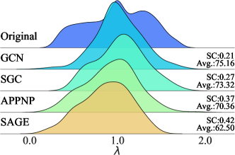
(a) LEDs in various architectures

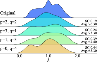
(b) LEDs in BWGNN [80]

Figure 2: (a): Illustrations of the LEDs (use the density plotting, each peak represents the LED of a graph), SC, and Avg. (average test performances on GCN, SGC, APPNP, and SAGE) in various architectures. (b): Evaluation of these three metrics in frequency-adaptive BWGNN. We empirically find that the LED shifts (i.e., SC) are high-consistent with Avg. performances, thus SC could be a good indicator to evaluate the performance of the condensed graph.

LED analysis of previous work. First, we define $\eta^{\mathcal{G}}$ and $\eta^{\mathcal{S}}$ as the LED of the original graph and condensed graph, respectively. Then the LED shift of the above two graphs can be formulated as: $||\eta^{\mathcal{G}}-\eta^{\mathcal{S}}||=||\sum_{i=1}^{N}\eta_{i}(\mathbf{X},\tilde{\mathbf{L}})-\sum_{j=1}^{N^{\prime}}\eta_{j}(\mathbf{X^{\prime}},\tilde{\mathbf{L}}^{\prime})||$. In GCond [35], the matching function $\mathrm{M}$ defaults as the MSE loss. Therefore, the objective of GCond can be written as $||\theta_{\mathcal{G}}-\theta_{\mathcal{S}}||\leq\epsilon$, where $\epsilon$ is a small number as expected. Incorporating such an objective in the LED shift formula, the lower bound is shown as follows.

Proposition 1.

Refer to [1, 4, 80], the GNN can be recognized as the bandpass filter. Assume the frequency response area of GNN is $(a,b)$, where $(a,b)$ is architecture-specific. The lower bound of GCond is shown in Eq. (3). Detailed proof can be found in Appendix B.1.

$$||\eta^{\mathcal{G}}-\eta^{\mathcal{S}}||\geq\epsilon+\sum_{i=1}^{a}||\boldsymbol{\bar{x}_{i}^{2}}-\boldsymbol{\bar{x}_{i}^{{}^{\prime}2}}||+\sum_{j=b}^{N^{\prime}}||\boldsymbol{\bar{x}_{j}^{2}}-\boldsymbol{\bar{x}_{j}^{{}^{\prime}2}}||.$$ (3)

According to Eq. (3), we find the lower bond of LED in GCond is related to the frequency response area $(a,b)$ (i.e., specific GNN). For example, GCN [38] or SGC  [90] (utilized in GCond) is a low-pass filter [1], which emphasizes the lower Laplacian energy. As shown in Fig. 1(a), the $\mathbf{A^{\prime}}$ is built upon the learned “low-frequency” feature $\mathbf{X^{\prime}}$, which may fail to generalize to cross-architectures (i.e., high-pass filters) and specific tasks.

Exploration of the effects of LED shift on the generalization performance. Although the LED shift phenomenon occurs in GCond, quantifying the LED shift is challenging because $\mathcal{G}$ and $\mathcal{S}$ have different numbers of nodes. To enable comparison, we follow an intuitive assumption that two nodes with similar eigenvalue distribution proportions can be aligned in comparison. Thus, we first convert LEDs of $\mathcal{G}$ and $\mathcal{S}$ into probability distributions using the Kernel Density Estimation (KDE) method [58]. Then we quantify the LED shifts as the distance of the probability distributions using the Jensen-Shannon (JS) divergence [45]. We define the LED shift coefficient ($SC$) in Definition 2:

Definition 2 (LED shift coefficient, $SC$).

The LED shift coefficient between $\mathcal{G}$ and $\mathcal{S}$ is:

$$SC=\operatorname{JS}\left(\frac{1}{|V_{\mathcal{G}}|h}\sum_{\bar{x}_{i}\in X_{\mathcal{G}}}K(\frac{x-\bar{x}_{i}}{h})\Big{|}\Big{|}\frac{1}{|V_{\mathcal{S}}|h}\sum_{\bar{x}_{j}\in X_{\mathcal{S}}}K(\frac{x-\bar{x}_{j}}{h})\right),$$ (4)

where the $\operatorname{JS}(\cdot||\cdot)$ denotes the JS-divergence, the $|V_{\mathcal{G}}|$ and the $|V_{\mathcal{S}}|$ is the number of the nodes to corresponding graphs, the $K(\cdot)$ represents the Gaussian kernel function with bandwidth parameter $h$. $SC\in[0,1]$ reflects the divergence between $\mathcal{G}$ and $\mathcal{S}$ (a smaller $SC$ indicates more similar).

In Fig. 2, we empirically study the influences of $SC$ in two settings: various GNNs in Fig. 2(a) and fixed BWGNN [80] with adaptive bandpass in Fig. 2(b). Based on the results in Fig. 2, We have several observations: (1) The entangled learning paradigm that building structure (i.e., adjacency matrix) upon on feature matrix will significantly lead to the LED shift phenomenon. (2) The positive correlation exists between the LED shift and the generalization performance of the condensed graph. (3) Preserving more information about the original graph structure may alleviate the LED shift phenomenon and improve the generalization performance of the condensed graph.

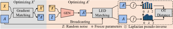
Figure 3: The Training pipeline of the SGDD (left). We first fix $\mathbf{A^{\prime}}$ to optimize $\mathbf{X^{\prime}}$ through the gradient matching strategy and we broadcast the supervision of $\mathbf{A}$ to the generation of the graph structure $\mathbf{A^{\prime}}$. To mitigate the Laplacian Energy Distribution (LED) shift phenomenon, we propose the LED Matching strategy to optimize the $\mathbf{A^{\prime}}$, which optimizes the learned structure with the optimal transport (OT) distance (right).

4 Structure-broadcasting Graph Dataset Distillation

In this section, we first present the pipeline and overview of SGDD in Fig. 3. Then, we introduce two modules of SGDD. Finally, we summarize the training pipeline of our SGDD.

4.1 Learning graph structure via graphon approximation

To prevent overlooking the original structure $\mathbf{A}$ from $\mathcal{G}$, we broadcast $\mathbf{A}$ as supervision for the generation of $\mathbf{A^{\prime}}$. Considering the different shapes between $\mathbf{A}$ and $\mathbf{A^{\prime}}$ ($N^{\prime}\ll N$), we introduce graphon [20, 67, 16, 31, 92] to distill the original structure information to the condensed structure $\mathbf{A^{\prime}}$. Specifically, given random noise $\mathcal{Z}(N^{\prime})\in\mathbb{R}^{N^{\prime}\times N^{\prime}}$ as the input coordinates, through the generative model, we then synthesize an adjacency matrix $\mathbf{A^{\prime}}$ with $N^{\prime}$ nodes. This process can be formulated as $\mathbf{A^{\prime}}=\mathrm{GEN}(\mathcal{Z}(N^{\prime});\Phi)$, where the $\mathrm{GEN}(\cdot)$ is a generative model with parameter $\Phi$, and the optimization process is then defined as:

$$\mathcal{L}_{\textbf{structure}}=\mathrm{Distance}(\mathbf{A},\mathrm{GEN}(\mathcal{Z}(N^{\prime});\Phi)),$$ (5)

where $\mathbf{A}$ is supervision and $\mathrm{Distance}$$(\cdot)$ is a metric that measure the difference of $\mathbf{A}$ and $\mathbf{A^{\prime}}$. The details of $\mathrm{Distance}$$(\cdot)$ can be found in Sec. 4.2. To avoid overlooking of the inherent relation  [30, 71] between $\mathbf{A^{\prime}}$ and the corresponding node information (i.e., $\mathbf{X^{\prime}}$ and $\mathbf{Y^{\prime}}$), we jointly input $\mathbf{X^{\prime}}$ and $\mathbf{Y^{\prime}}$ as conditions to generate $\mathbf{A^{\prime}}$. Therefore, the final version of the generative model can be written as $\mathbf{A^{\prime}}=\mathrm{GEN}(\mathcal{Z}(N^{\prime})\oplus\mathbf{X^{\prime}}\oplus\mathbf{Y^{\prime}};\Phi)$, the $\oplus$ denotes the concatenate operation.

To study the performance of SGDD in the above paradigm, we theoretically prove the upper bound of LED shift in SGDD  by invoking graphon theory. The result can be presented as follows.

Proposition 2.

The upper bound of the LED shift on SGDD  is shown as:

$$||\eta^{\mathcal{G}}-\eta^{\mathcal{S}}||\leq\delta_{\square}(W_{\mathbf{A}},\mathbf{A^{\prime}}),$$ (6)

where $\delta_{\square}$ denotes the cut distance [52] and $W_{\mathbf{A}}$ is the graphon of $\mathbf{A}$. See details in Appendix B.2.

Note minimizing the upper bound of Eq. (6) is equal to optimizing the $L_{structure}$ on Eq. (5). Compared to the lower bound in (Eq. (3)), our upper bound is not related to any frequency response of specific GNN (i.e., the terms of $\sum_{i=1}^{a}||\boldsymbol{\bar{x}_{i}^{2}}-\boldsymbol{\bar{x}_{i}^{{}^{\prime}2}}||+\sum_{i=b}^{N^{\prime}}||\boldsymbol{\bar{x}_{i}^{2}}-\boldsymbol{\bar{x}_{i}^{{}^{\prime}2}}||$). As a result, SGDD  may perform better than the previous work, especially in the cross-architecture setting and specific tasks.

4.2 Optimizing the graph structure via optimal transport

To mitigate the LED shift between $\mathbf{A}$ and $\mathbf{A^{\prime}}$, ideally, we can directly minimize the proposed $SC$. However, $SC$ requires an extremely time-consuming ($O(N^{3}$)) [4, 56] eigenvalue decomposition operation. Therefore, we propose the LED Matching strategy based on the optimal transport theory to form an efficient optimizing process.

Recall in the Eq.(4) of calculating $SC$, we first decompose the eigenvalue, followed by aligning the node through the JS divergence, which essentially compares the distribution proportions. The key point is to decide the node mapping strategy to align such two graphs. Alternatively, assuming we know the prior distribution of the alignment of $\mathcal{S}$ (i.e., we know the bijection of nodes in $\mathcal{S}$ to the $\mathcal{G}$) and denoting such alignment as $\mathcal{S}*$, we can directly measure the distance between $\mathcal{G}$ and $\mathcal{S}*$ by employing the 2-Wasserstein metric[96, 54].

$$||\eta^{\mathcal{G}}-\eta^{\mathcal{S}*}|| =W_{2}^{2}\left(\eta^{\mathcal{G}},\eta^{\mathcal{S}*}\right)$$ (7)

Furthermore, following the assumption in previous work[54, 96], we have $\eta^{G}\sim\mathcal{N}\left(0,L_{\mathcal{G}}^{\dagger}\right)$ and $\eta^{S}\sim\mathcal{N}\left(0,L_{\mathcal{S}*}^{\dagger}\right)$. Then, the Eq.(7) have a closed-form expression[96] as follows:

$$||\eta^{\mathcal{G}}-\eta^{\mathcal{S}*}|| =N\operatorname{tr}\left(L_{\mathcal{G}}^{\dagger}\right)+N^{\prime}\operatorname{tr}\left(L_{\mathcal{S}*}^{\dagger}\right)-2\operatorname{tr}\left(\sqrt{L_{\mathcal{S}*}^{\frac{\ddagger}{2}}L_{\mathcal{G}}^{\dagger}L_{\mathcal{S}*}^{\frac{\dagger}{2}}}\right),$$ (8)

the $L_{\mathbf{\cdot}}^{\dagger}$ denotes the Laplacian pseudo-inverse operation and the $\operatorname{tr}$ indicates the trace operation of matrix. Therefore, even though we could not know the actual mapping strategy $\mathcal{S}*$, we can use the infimum of all possible strategies as a proxy solution. Formally, following the prior work [54], we employ the function $T$ as a transport plan in the metric space $\mathcal{X}$ to represent all feasible mapping strategies. Then, we use the $T_{\#}\eta^{\mathcal{S}}$ to represent the pushing forward process of transferring the distribution of $\eta^{\mathcal{S}}$ to the $\eta^{\mathcal{G}}$. As a result, the distance can be regarded as finding the infimum.

$$||\eta^{\mathcal{G}}-\eta^{\mathcal{S}}|| =\inf_{T_{\#}\eta^{\mathcal{S}}=\eta^{\mathcal{G}}}\int_{\mathcal{X}}\|x-T(x)\|^{2}d\eta^{\mathcal{S}}(x)$$ (9)

$$=N^{\prime}\operatorname{tr}(L_{\mathcal{S}}^{\dagger})-2\operatorname{tr}\left(\left((L_{\mathcal{S}}^{\dagger})^{1/2}P^{T}L_{\mathcal{G}}^{\dagger}P\left(L_{\mathcal{S}}^{\dagger}\right)^{1/2}\right)^{1/2}\right).$$

Here, due to the transport plan $T$ is impractical in optimizing, following the previous work[96], we use $P\in\mathbb{R}^{N^{\prime}\times N}$ denotes as a free parameter serving as the direct mapping strategy between nodes. Thus, the $\operatorname{Distance}$ in the Eq. (5) could be directly optimized by the Eq.(9) (i.e., use the $P$ represents all possible mapping strategies, the optimizing of $P$ is equal to choosing a more optimal mapping strategy). In the experimental setting, we use the Sinkhorn-Knopp[9] algorithm to optimize $P$.

The overall time complexity is reduced to the $O(N^{\omega})\leq O(N^{2.373})$[96]. Note that the $L_{\mathcal{G}}^{\dagger}$ may be too large for computing, so we empirically sample a medium size (e.g., 2,000 nodes) sub-structure in the experiment and ablate its influence in Appendix C.7.

4.3 Training pipeline of SGDD

As illustrated in Fig. 1(d) and Fig. 3, we commence by introducing a novel graph structure learning paradigm termed "graphon approximation". This paradigm integrates both the feature $X^{\prime}$ and auxiliary information $Z$ to generate the structure. Subsequently, the learned structure $A^{\prime}$ is forced to be closer to the original graph structure $A$ in terms of Laplacian energy distribution.

Additionally, our proposed methodology, SGDD, implements a bi-loop optimization schema. Within this framework, we concurrently optimize the parameters $X^{\prime}$ and $A^{\prime}$. More specifically, the refinement of $X^{\prime}$ is achieved through a gradient matching strategy, whereas the $A^{\prime}$ is enhanced using the LED matching technique. During each step, the other component is frozen to ensure effective refinement.

Our overall training loss function can be summarized as $\mathcal{L}=\mathcal{L}_{feature}+\alpha\mathcal{L}_{structure}+\beta||\mathbf{A}||_{2}$, where the $||\mathbf{A}||_{2}$ is proposed as a sparsity regularization term and $\mathcal{L}_{feature}$ denotes the gradient matching strategy [35]. $\alpha$ and $\beta$ are trade-off parameters, we study their sensitiveness in the Sec. 5.3. The algorithm can be found in Appendix C.3.

5 Experiments

Table 1: Comparisons to state-of-the-art methods. SGDD  achieves the highest results in most cases on node classification (NC), anomaly detection (AD), and link prediction (LP) tasks. We report test accuracy (%) on NC datasets (including Citeseer, Cora, Ogbn-arxiv, Flickr, and Reddit), F1-macro (%) on AD datasets (including YelpChi and Amazon), and AUC (%) on LP datasets (including Citeseer-L and DBLP). Bold entries are best results, underline mark the runner-ups.

	Dataset	Ratio ($r$)	Random	Herding	K-Center	Coarsening	GDC	Gcond	SGDD	Whole
NC	Citeseer [39]	0.90%	54.4±4.4	57.1±1.5	52.4±2.8	52.2±0.4	66.8±1.5	70.5±1.2	69.5±0.4	71.7±0.1
		1.80%	64.2±1.7	66.7±1.0	64.3±1.0	59.0±0.5	66.9±0.9	70.6±0.9	70.2±0.8
		3.60%	69.1±0.1	69.0±0.1	69.1±0.1	65.3±0.5	66.3±1.5	69.8±1.4	70.3±1.7
	Cora [39]	1.30%	63.6±3.7	67.0±1.3	64.0±2.3	31.2±0.2	67.3±1.9	79.8±1.3	80.1±0.7	81.2±0.2
		2.60%	72.8±1.1	73.4±1.0	73.2±1.2	65.2±0.6	67.6±3.5	80.1±0.6	80.6±0.8
		5.20%	76.8±0.1	76.8±0.1	76.7±0.1	70.6±0.1	67.7±2.2	79.3±0.3	80.4±1.6
	Ogbn-arxiv [28]	0.05%	47.1±3.9	52.4±1.8	47.2±3.0	35.4±0.3	58.6±0.4	59.2±1.1	60.8±1.3	71.4±0.1
		0.25%	57.3±1.1	58.6±1.2	56.8±0.8	43.5±0.2	59.9±0.3	63.2±0.3	65.8±1.2
		0.50%	60.0±0.9	60.4±0.8	60.3±0.4	50.4±0.1	59.5±0.3	64.0±0.4	66.3±0.7
	Flickr [99]	0.10%	41.8±2.0	42.5±1.8	42.0±0.7	41.9±0.2	46.3±0.2	46.5±0.4	46.9±0.1	47.2±0.1
		0.50%	44.0±0.4	43.9±0.9	43.2±0.1	44.5±0.1	45.9±0.1	47.1±0.1	47.1±0.3
		1.00%	44.6±0.2	44.4±0.6	44.1±0.4	44.6±0.1	45.8±0.1	47.1±0.1	47.1±0.1
	Reddit [25]	0.01%	46.1±4.4	53.1±2.5	46.6±2.3	40.9±0.5	88.2±0.2	88.0±1.8	90.5±2.1	93.9±0.0
		0.05%	58.0±2.2	62.7±1.0	53.0±3.3	42.8±0.8	89.5±0.1	89.6±0.7	91.8±1.9
		0.50%	66.3±1.9	71.0±1.6	58.5±2.1	47.4±0.9	90.5±1.2	90.1±0.5	91.6±1.8
AD	YelpChi  [66]	0.05%	41.8±0.3	46.1±0.9	49.3±1.1	46.2±2.1	47.9±1.1	48.6±3.7	56.2±1.8	61.1±1.8
		0.10%	43.7±1.2	47.1±1.2	44.2±1.8	47.5±1.8	50.2±2.1	49.6±1.8	58.1±2.3
		0.20%	45.9±2.2	46.4±0.8	47.5±0.4	49.1±1.2	49.7±2.0	50.1±2.8	59.7±1.8
	Amazon [101]	0.02%	76.2±0.8	74.1±0.9	73.4±2.1	75.2±2.9	74.1±1.9	77.9±3.1	83.3±2.6	89.5±0.9
		0.20%	76.4±1.6	76.5±2.3	74.2±1.1	76.8±1.0	78.2±2.1	78.1±1.9	84.8±1.7
		2.00%	78.2±0.9	77.2±1.8	73.8±2.2	77.8±2.8	79.3±3.1	79.2±2.0	86.9±2.1
LP	Citeseer-L [95]	0.90%	56.8±0.8	63.1±1.3	78.3±2.6	76.9±0.8	81.5±2.5	83.4±1.9	86.4±1.6	96.8±1.8
		1.80%	61.4±1.8	63.3±1.8	79.1±1.8	77.4±1.7	83.4±1.6	83.8±2.1	87.2±2.1
		3.60%	63.5±0.9	64.7±1.7	80.6±2.7	78.4±0.4	84.2±2.1	83.1±2.7	87.1±1.2
	DBLP [81]	0.05%	64.1±2.6	65.8±0.7	72.4±1.6	77.8±1.3	78.9±2.1	77.2±2.1	81.3±2.8	84.2±0.7
		0.25%	68.3±1.4	71.2±1.7	74.9±2.8	76.9±0.9	77.5±1.9	78.6±1.2	82.1±1.9
		0.50%	68.7±2.6	74.3±0.8	75.2±0.6	76.8±2.1	77.6±2.1	79.9±1.9	82.1±1.8

5.1 Datasets and implementation details

Datasets. We evaluate SGDD on five node classification datasets: Cora [39], Citeseer [39], Ogbn-arxiv [28], Flickr [99], Reddit [25], two anomaly detection datasets: YelpChi [66], Amazon [101], and two link prediction datasets: Citeseer-L [95], DBLP [81]. For the node classification and anomaly detection tasks, we follow the public settings [17] of train and test. To make a fair comparison, we also follow the previous setting [100, 81], we randomly split 80% nodes for training, 10% nodes for validation, and the remaining 10% for testing. To avoid data leakage, we only utilize 80% training samples for condensation. More details of each dataset can be found in Appendix C.1.

Implementation details. Without specific designation, in the condense stage, we adopt the 2-layer GCN with 128 hidden units as the backbone, and we adopt the settings on [92], which use 2-layer MLP to represent the structure generative model (i.e., $\mathrm{GEN}$). The learning rates for structure and feature are set to 0.001 (0.0001 for Ogbn-arxiv and Reddit) and 0.0001, respectively. We set $\alpha$ to 0.1, and $\beta$ to 0.1. In the evaluation stage, we train the same network for 1,000 epochs on the condensed graph with a learning rate of 0.001. Following the settings in [35], we repeat all experiments ten times and report average performance and variance. More details can be found in Appendix C.2.

5.2 Comparison with state-of-the-art methods

We compare our proposed SGDD with six baselines: Random, which randomly selected nodes to form the original graph, corset methods (Herding [88] and K-Center [70]), graph coarsening methods (Corasening [29]), and the state-of-the-art graph condensation methods (GCond [35]). GDC is proposed as a baseline in [35], where cosine similarity is added as a constraint to generate the structure of the condensed graph.

In Table 1, we present the performance metrics including accuracy, F1-macro, and AUC. For clarity and simplicity, percentages are represented without the $\%$ symbol, and variance values are also provided.

Based on the results, we have the following observations: 1) Our proposed SGDD achieves the highest results in most settings, which shows the superiority and generalization of our method. 2) On anomaly detection datasets, the improvements are more significant than other tasks, i.e., improving GCond with 9.6% and 7.7% on YelpChi and Amazon datasets, which can be explained that our method captures the structure information from the original graph dataset more efficiently.

Table 2: Results of cross-architecture setting, we test condensed graphs in APPNP, Cheby, GCN, GraphSAGE, and SGC. Avg. and Std.: the average performance and the standard deviation of the results, the $\Delta$(%) denotes the improvements upon the GDC. We mark the best performance by bold.

		Architectures							Statistics
Datasets	Methods	MLP [11]	GAT [82]	APPNP [40]	Cheby [13]	GCN [39]	SAGE [25]	SGC [90]	Avg.	Std.	$\Delta$(%)
	GDC	50.3	54.8	81.2	77.5	89.5	89.7	90.5	76.2	16.9	-
	GCond	42.5	60.2	87.8	75.5	89.4	89.1	89.6	76.3	18.5	$\uparrow\pagecolor[HTML]{C6EFFC}0.1$
Reddit [25]	Ours	56.1	74.4	89.2	78.4	89.4	89.4	89.4	80.9	12.6	$\uparrow\pagecolor[HTML]{C6EFFC}\textbf{4.7}$
	GDC	67.2	64.2	67.1	67.7	67.9	66.2	72.8	67.6	2.6	-
	GCond	73.1	66.2	78.5	76	80.1	78.2	79.3	75.9	4.9	$\uparrow\pagecolor[HTML]{C6EFFC}8.3$
Cora [39]	Ours	76.7	75.8	78.4	78.5	79.8	80.4	78.5	78.3	1.6	$\uparrow\pagecolor[HTML]{C6EFFC}\textbf{10.7}$
	GDC	74.4	76.8	77.4	76.7	78.9	74.8	78.4	76.8	1.7	-
	GCond	75.3	77.6	78.9	76.1	79.6	77.4	79.9	77.8	1.7	$\uparrow\pagecolor[HTML]{C6EFFC}1.1$
DBLP [81]	Ours	78.4	79.6	80.1	80.6	82.1	80.7	81.4	80.4	1.2	$\uparrow\pagecolor[HTML]{C6EFFC}\textbf{3.6}$
	GDC	30.7	36.4	43.7	41.5	49.6	47.4	50.1	42.8	7.2	-
	GCond	48.9	31.8	46.7	48.6	50.1	42.5	48.7	45.3	6.5	$\uparrow\pagecolor[HTML]{C6EFFC}2.6$
YelpChi [66]	Ours	54.2	56.4	58.2	56.8	59.7	54.1	56.7	56.6	2.0	$\uparrow\pagecolor[HTML]{C6EFFC}\textbf{13.8}$

Table 3: Comparison of the cross-architecture generalization performance between GCond and SGDD on Ogbn-arxiv. Bold entries are the best results. $\uparrow$/$\downarrow$: our method show increase or decrease performance.

C\T	APPNP	Cheby	GCN	SAGE	SGC
	GCond / SGDD	GCond / SGDD	GCond / SGDD	GCond / SGDD	GCond / SGDD
APPNP	60.3 / 60.2$\downarrow$	51.8 / 53.2$\uparrow$	59.9 / 62.4$\uparrow$	59.0 / 60.2$\uparrow$	61.2 / 60.4$\downarrow$
Cheby	57.4 / 58.5$\uparrow$	53.5 / 55.8$\uparrow$	57.4 / 65.3$\uparrow$	57.1 / 57.0$\downarrow$	58.2 / 60.2$\uparrow$
GCN	59.3 / 60.1$\uparrow$	51.8 / 53.7$\uparrow$	60.3 / 64.2$\uparrow$	60.2 / 61.2$\uparrow$	59.2 / 59.8$\uparrow$
SAGE	57.6 / 58.9$\uparrow$	53.9 / 53.8$\uparrow$	58.1 / 63.8$\uparrow$	57.8 / 61.8$\uparrow$	59.0 / 61.1$\uparrow$
SGC	59.7 / 60.0$\uparrow$	49.5 / 52.3$\uparrow$	59.2 / 62.2$\uparrow$	58.9 / 62.9$\uparrow$	60.5 / 61.5$\uparrow$

Table 4: Neural Architecture Search. Methods are compared in validation accuracy correlation and test accuracy on obtained architecture.

	Pearson Correlation / Performance (%)
Dataset	Random	GCond	SGDD	Whole Per. (%)
Ogbn-arxiv	0.63 / 71.1	0.64 / 71.2	0.67 / 71.6	71.9
YelpChi	0.43 / 56.7	0.48 / 58.4	0.56 / 60.6	61.1
DBLP	0.58 / 81.2	0.62 / 83.8	0.68 / 84.0	84.2

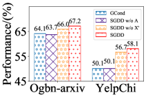
(a) Ablation of $\mathbf{X^{\prime}}$ and $\mathbf{A}$.

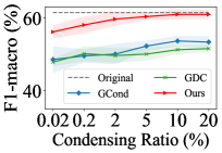
(b) Evaluation of $r$(%)

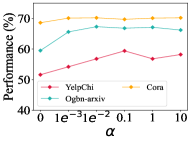
(c) Evaluation of $\alpha$

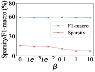
(d) Evaluation of $\beta$

Figure 4: (a) Ablation of components in SGDD. (b) Evaluation of the scalability of SGDD. (c) and (d): the trade-off parameters analysis on $\alpha$ and $\beta$.

5.3 Ablation Study

Cross-architecture generalization analysis. To evaluate the generalization ability of SGDD on unseen architectures, we conduct experiments that train on the condensed graph with different architectures and report their performances in Tab. 2. Here, the condensed graph is obtained by optimizing SGDD with SGC [90]. We test its cross-architecture generalization performances on 2-layer-MLP [11], GAT [82], APPNP [40], Cheby [13], GCN [39], and SAGE [25]. To better understand, we also show several statistics metrics, including Avg., Std., and $\Delta$. SGDD and GCond improves GDC significantly, which indicates there exists a large difference between graph dataset condensation and vision dataset distillation, i.e., the structure information should be specially considered. Compared to GCond, the improvement of our method is up to 11.3%, demonstrating the effectiveness of broadcasting the original structure to the condensed graph structure generation. More experiments on other datasets can be found in Appendix C.6.

Versatility of SGDD. Following the setting of GCond [35], we also study whether our proposed SGDD is robust on various architectures. We first condense the Ogbn-arxiv graph dataset with five architectures, including APPNP [40], Cheby [13], GCN [39], SAGE [25], and SGC [90], respectively. Then, we evaluate these condensed graphs on the above five architectures and report their performances in Tab. 4. The experiment results show that SGDD achieves non-trivial improvements than GCond in most cases, which demonstrates the strong versatility of our method.

Evaluation on neural architecture search. Similar to vision dataset distillation, graph dataset distillation is also expected to reduce the high cost of neural architecture search (NAS). In order to make a fair comparison, we follow the experimental setting in [35]: searching architectures on condensed Obgn-arxiv, YelpChi, and DBLP datasets with 0.25%, 0.2%, and 0.5% condensing ratios. We report Pearson correlation [43] and performance of random, GCond, and SGDD in Tab. 4. Our SGDD consistently achieves the highest Pearson correlations as well as performances, which indicates the architectures searched by our method are efficient for the whole graph dataset training.

Evaluation of components in SGDD. To explore the effect of the conditions (mentioned in Sec. 4.1) in the condensed graph generation, we design the ablation study of $\mathbf{X^{\prime}}$ and $\mathbf{A}$. As shown in Fig 4(a), $\mathbf{X^{\prime}}$ and $\mathbf{A}$ are complementary with each other. SGDD w/o $\mathbf{A}$ performs poorly on Obgn-arxiv and YelpChi datasets, which demonstrates the effect of original graph structure information. Jointly using $\mathbf{X^{\prime}}$ and $\mathbf{A}$ achieves the highest performances on both datasets, improves GCond with 3.1% on Ogbn-arxiv, and 8.0% on YelpChi.

Evaluation of the scalability of SGDD.

To investigate the scalability of SGDD, we evaluate the SGDD on various condensing ratios with $r\in\{0.02,0.2,2,5,10,20\}$. As shown in Fig. 4(b), the performance of our method continuously increase as the condensing ratio rises, which indicates the strong scalability of our method. GCond obtains marginal improvements than GDC at all ratios while our SGDD outperforms them significantly. More important, SGDD achieves lossless performance as training on the original graph data when the condensing ratio is 10%.

Exploring the sensitivity of $\alpha$ and $\beta$. $\alpha$ is a parameter of $\mathcal{L}_{structure}$ that reflects the weight of original graph structure. We conduct experiments to test its sensitivity on YelpChi, Cora, and Ogbn-arxiv. As shown in Fig. 4(c), we empirically find that the performance of our SGDD is not sensitive to the $\alpha$. Specifically, compared to the case that $\alpha$ is zero, we have a significant improvement, which proves the effectiveness of our method. Another finding is that the $\alpha$ should be set higher on anomaly detection than on node classification tasks. It could be explained by the original graph structure information being more important on the complex task (such as anomaly detection). We define $\beta$ as a regularization coefficient to control the sparsity of the condensed graph. As shown in Fig. 4(d), we evaluate the $\beta$ from 0 to 10 on the YelpChi dataset. The results illustrate that the performance is not sensitive with $\beta$ and achieve the highest result (F1-macro) when $\beta$ is set to our default value ($\beta=0.1$). More experiments can be found in Appendix C.5.

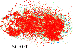
(a) Original Ogbn-arxiv

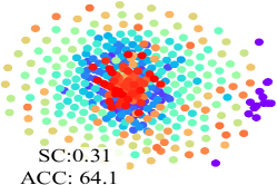
(b) Condensed by GCond [35]

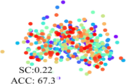
(c) Condensed by SGDD 

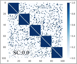
(d) Original synthetic graph

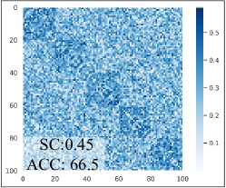
(e) Condensed by GCond [35]

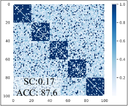
(f) Condensed by SGDD 

Figure 5: Visualizations of the real dataset (a), synthetic dataset (d), and the corresponding condensed graph obtained by GCond (b, e) and SGDD  (c, f). The condensing ratio $r$ is set to 0.5%.

5.4 Visualizations

To better understand the effectiveness of our SGDD, we visualize the condensed graphs of GCond and SGDD that are synthesized from real and synthetic graph datasets. For the synthetic graph dataset, we use the Stochastic Block Model (SBM) [27] to synthesize graphs with $5$ community (Fig. 5(d)). As shown in Fig. 5, one can find that our method consistently achieves better performances and $SC$. SGDD reduces 29.0% (comparing 5(b) and 5(c)) and 62.2% (comparing 5(e) and 5(f)) $SC$ on Ogbn-arxiv and synthetic datasets.

Visually, the condensed graphs of our method preserve the original graph structure information obviously better than GCond (see the second row of Fig. 5), which proves SGDD is a powerful graph dataset distillation method.

6 Conclusion

We present SGDD, a novel framework for graph dataset distillation via broadcasting the original structure information to the generation of the synthetic one. SGDD shows its robustness on various tasks and datasets, achieving state-of-the-art results on YelpChi, Amazon, Ogbn-arxiv, and DBLP. SGDD reduces the scale of the Yelpchi dataset by 1,000 times while maintaining 98.6% as training on the original data. We provide sufficient experiments and theoretical analysis in this paper and hope it can help the following research in this area.

Limitations and future work: Although broadcasting the original information to the generated graph shows remarkable success, some informative properties (e.g., the heterogeneity) may lose during the current condense process, which results in sub-optimal performance in the downstream tasks. We are going to explore a more general method in the future.

Appendix A More Preliminary and Related Work

A.1 More preliminary

Graphon. A graphon [41, 32, 52] is a bounded, symmetric, and Lebesgue measurable function, denote as $W:\Omega^{2}\to[0,1]$, where $\Omega$ is a probability measure space. By randomly selecting points $\{v_{0},v_{1},\dots,v_{n}\}$ from $\Omega$, we can create a graph of any size by connecting each point with an edge weight $e_{ij}=W(v_{i},v_{j})$. Formally, we can follow the random sampling process to get arbitrarily sized ($n$) graphs :

$$v_{i} \sim\mathrm{Uniform}(\Omega),~{}\text{for}~{}i=1,\cdots,n,$$ (10)

$$e_{ij} \sim\mathrm{Bernoulli}(W(v_{i},v_{j})),~{}\text{for}~{}i,j=1,\cdots,n.$$

Conventionally, we use a deterministic setting to select the node, e.g., the fixed grid $v_{i}=\frac{i-1}{n}$. Graphs derived from the same graphon share several important properties for statistical analysis: such as density [20], clustering coefficient [67], and degree distribution [69], which motivate us to broadcast the original graph structure information to the condensed graph via the graphon approximating.

A.2 More related work

Graph structure learning. Graph structure learning [18, 33, 8, 107, 53] also aims at jointly optimizing the graph structure and the corresponding node features. Most of these methods learn the new structure based on the certain constraints (e.g., low-rank [89], sparsity [8], feature smoothness [33], and homophily [107]). However, these methods are unable to learn a new structure with a significantly reduced node size. In contrast, our method can synthesize a smaller graph structure while simultaneously constructing new node features. The obtained small but informative graph can reduce the training cost in the downstream tasks.

Appendix B Proofs

B.1 Proof of Proposition 1

Proof.

First, the gradient matching objective in GCond [35] can be shown as:

$$\mathrm{Match}( \nabla_{\boldsymbol{\theta}}\mathcal{L}_{cls}\left(\text{GNN}_{\boldsymbol{\theta}}({\bf A},{\bf X}),{\bf Y}\right)), \nabla_{\boldsymbol{\theta}}\mathcal{L}_{cls}\left(\text{GNN}_{\boldsymbol{\theta}}(\mathbf{A}^{\prime},{\bf X^{\prime}}),{\bf Y^{\prime}}\right)),$$ (11)

where $\mathrm{Match}(\cdot)$ is the matching function that measures the distance of the two gradients. $\mathbf{\theta}$ represents the parameters of the GNN, the $\nabla$ denotes the gradient in the backpropagation process, and the $\mathcal{L}_{cls}$ represents the loss function that is used in the supervised tasks, i.e., cross-entropy loss. Following the discussion in the  [4, 1, 80], the GNN can be viewed as a bandpass filter in the spectral domain. Expanding the GNN in the spectral domain, we can rewrite the objective as:

$$\Big{|}\Big{|}\int_{i=0}^{N}\mathbf{U}_{\mathbf{A}}\operatorname{diag}(\mathrm{T}_{i}(\boldsymbol{\lambda_{\mathbf{A}}}))\mathbf{U}_{\mathbf{A}}^{\top}\mathbf{X}-\int_{j=1}^{N^{\prime}}\mathbf{U}_{\mathbf{A}^{\prime}}\operatorname{diag}\left(\mathrm{T}_{j}(\boldsymbol{\lambda_{\mathbf{A}^{\prime}}})\right)\mathbf{U}_{\mathbf{A}^{\prime}}^{\top}\mathbf{X}^{\prime}\Big{|}\Big{|}\leq\epsilon,$$ (12)

where the $\mathrm{T}(\boldsymbol{\lambda})$ denotes the frequency response of the given GNN, the $\boldsymbol{\lambda}$ and the $\mathbf{U}$ is the eigenvalue and eigenvector of the corresponding graph, respectively. Note we drop the $\nabla$, the $\mathcal{L}_{cls}$, and the $\mathbf{Y}$ ($\mathbf{Y}^{\prime}$) terms because they can be viewed as the intermediate process [104, 106] in approximating to Eq.(12). We use the MSE [35] as the matching function $\mathrm{Match}(\cdot)$ for simplicity.

To simplify $\mathrm{T}(\mathbf{\boldsymbol{\lambda}})$, without loss of generality, we assume the bandwidth of the specific GNN’s frequency response is (a, b), which intuitively indicates that only the signal of frequency in (a, b) can pass through the filter on the graph. Then the Eq. (12) can be written as:

$$\Big{|}\Big{|}\int_{i=0}^{N}\int_{k=a}^{b}\mathbf{U}_{\mathbf{A}}\operatorname{diag}(\boldsymbol{\lambda_{\mathbf{A}}}^{k})\mathbf{U}_{\mathbf{A}}^{\top}\mathbf{X}-\int_{j=1}^{N^{\prime}}\int_{k=a}^{b}\mathbf{U}_{\mathbf{A}^{\prime}}\operatorname{diag}(\boldsymbol{\lambda_{\mathbf{A}^{\prime}}}^{k})\mathbf{U}_{\mathbf{A}^{\prime}}^{\top}\mathbf{X}^{\prime}\Big{|}\Big{|}\leq\epsilon,$$ (13)

we further combine the first integration, the objective can thus be summarized as:

$$\Big{|}\Big{|}\int_{k=a}^{b}\left(\mathbf{U}_{\mathbf{A}}\operatorname{diag}(\boldsymbol{\lambda_{\mathbf{A}}}^{k})\mathbf{U}_{\mathbf{A}}^{\top}\mathbf{X}-\mathbf{U}_{\mathbf{A}}\operatorname{diag}(\boldsymbol{\lambda_{\mathbf{A}^{\prime}}}^{k})\mathbf{U}_{\mathbf{A}^{\prime}}^{\top}\mathbf{X}^{\prime}\right)\Big{|}\Big{|}\leq\epsilon.$$ (14)

Then following the transformation in the spectral domain [1], we can briefly summarized:

$$\int_{i=a}^{b}||\bar{x}_{i}^{2}-\bar{x}_{i}^{{}^{\prime}2}||\leq\epsilon.$$ (15)

Take the Eq. (15) into the $\left\|\eta^{\mathcal{G}}-\eta^{\mathcal{S}}\right\|$:

$$||\eta^{\mathcal{G}}-\eta^{\mathcal{S}}||= ||\sum_{i=1}^{N}\bar{x}_{i}^{2}-\sum_{i=j}^{N^{\prime}}\bar{x}_{i}^{2}||$$ (16)

$$\geq \epsilon+||\sum_{i=1}^{a}\bar{x}_{i}^{2}-\sum_{j=1}^{a}\bar{x}_{j}^{2}||+||\sum_{i=b}^{N}\bar{x}_{i}^{2}-\sum_{j=b}^{N^{\prime}}\bar{x}_{j}^{2}||$$

$$\geq \epsilon+\sum_{i=1}^{a}\left\|\bar{x}_{i}^{2}-\bar{x}_{i}^{\prime 2}\right\|+\sum_{i=b}^{N^{\prime}}\left\|\bar{x}_{i}^{2}-\bar{x}_{i}^{\prime 2}\right\|.$$

Note the second inequality is under the assumption: intuitively, the overall distance of $\eta^{\mathcal{G}}$ and $\eta^{\mathcal{S}}$ should be larger than the condition that two graphs have the same size (i.e., $N=N^{\prime}$). ∎

B.2 Proof of Proposition 2

To prove Proposition 2, we first introduce the following notations and theorems in graphon theory.

The cut norm  [19, 52] is defined as:

$$\|W\|_{\square}:=\sup_{\mathcal{X},\mathcal{Y}\subset\Omega}\left|\int_{\mathcal{X}\times\mathcal{Y}}W(x,y)\mathrm{d}x\mathrm{d}y\right|,$$ (17)

where the $\Omega$ is the probability space of a graphon $W$, the supremum is taken over all measurable subsets $\mathcal{X}$ and $\mathcal{Y}$  [93]. Then the cut distance between $W_{1},W_{2}$ [52] can be defined as:

$$\delta_{\square}\left(W_{1},W_{2}\right):=\inf_{\phi\in\mathcal{S}_{\Omega}}\left\|W_{1}-W_{2}^{\phi}\right\|_{\square},$$ (18)

where the $\mathcal{S}_{\Omega}$ is the set of measure-preserving mappings from $\Omega$ to $\Omega$. When two graphons $W_{1},W_{2}$ have $\delta_{\square}(W_{1},W_{2})=0$, they can be seen equivalent, denoted as $W_{1}\cong W_{2}$.

To effectively approximate $W$ in the real world graphs, works [52, 31, 16] introduce an approximation named step function. Let $\mathcal{P}=\left(\mathcal{P}_{1},\ldots,\mathcal{P}_{K}\right)$ be a partition of $\Omega$ into $K$ measurable sets. The step function $W_{\mathcal{P}}:\Omega^{2}\mapsto[0,1]$ is defined as:

$$W_{\mathcal{P}}(x,y)=\sum_{k,k^{\prime}=1}^{K}w_{kk^{\prime}}1_{\mathcal{P}_{k}\times\mathcal{P}_{k^{\prime}}}(x,y),$$ (19)

where the $w_{kk^{\prime}}\in[0,1]$ and the indicator function $1_{\mathcal{P}_{k}\times\mathcal{P}_{k^{\prime}}}(x,y)$ is 1 if $(x,y)\in\mathcal{P}_{k}\times\mathcal{P}_{k^{\prime}}$, or it is 0.

To explore the relationship between step function and the $W$, we introduce the Weak Regularity Lemma as follows.

Theorem 1 (Weak Regularity Lemma [52]).

For every graphon $W\in\mathcal{W}$ and $K\leq 1$, there always exists a step function $W_{\mathcal{P}}$ with $|\mathcal{P}|=K$ steps such that

$$\left\|W-W_{\mathcal{P}}\right\|_{\square}\leq\frac{2}{\sqrt{\log K}}\|W\|_{L_{2}}.$$ (20)

We can further obtain the corollary that $\delta_{\square}\left(W,W_{\mathcal{P}}\right)\leq\frac{2}{\sqrt{\log K}}\|W\|_{L_{2}}$ as the $\delta_{\square}\left(W,W_{\mathcal{P}}\right)\leq\left\|W-W_{\mathcal{P}}\right\|_{\square}$. Intuitively, we can use any step function to approximate the ideal $W$ of real graphs.

Then to investigate the properties of the graphon in the spectral domain, following  [69, 83, 57, 68], we have the conclusion that:

$$\left|\left|S_{W}-S_{W_{\mathcal{P}}}\right|\right|\leq\left\|W-W_{\mathcal{P}}\right\|_{\square},$$ (21)

where the $S$ denotes the signal spectrum of the graphs [83] (i.e., the post-Graph-Fourier-Transform $\mathbf{U^{\top}X}$), Intuitively, the Eq. (21) shows that when the step function $W_{\mathcal{P}}$ is approximated to the $W$, they have similar signal spectrum.

Proof.

By combining the Theorem 1 and Eq.(21), the Proposition 2 replace the $W_{\mathcal{P}}$ with the $W_{\mathbf{A}}^{\prime}$, that’s because we use the generative model (i.e., $\mathrm{GEN}(\cdot)$) to approximate the step function $W_{\mathcal{P}}$. As we aim to learn the graphon of the original structure $\mathbf{A}$, the graphon $W$ can be rewrite as $W_{\mathbf{A}}$,

$$\left|\left|S_{W_{\mathbf{A}}}-S_{W_{\mathbf{A}}^{\prime}}\right|\right|\leq\left\|W_{\mathbf{A}}^{\prime}-W_{\mathbf{A}}\right\|_{\square}.$$ (22)

We notice that the $S$ here is related to the Laplacian energy distribution (LED), where the LED represents the probability distribution of the $S$, then we use the $\sum_{i=1}^{N}\bar{x}_{i}$ and $\sum_{j=1}^{N^{\prime}}\bar{x}_{j}$ to represent the summation of the original signal spectrum and the condensed one, respectively, we have:

$$||\eta^{\mathcal{G}}-\eta^{\mathcal{S}}|| =||\frac{S_{W_{\mathbf{A}}}}{\sum_{i=1}^{N}\bar{x}_{i}}-\frac{S_{W_{\mathbf{A}^{\prime}}}}{\sum_{j=1}^{N^{\prime}}\bar{x}_{j}}||$$ (23)

$$\leq\text{max}(\frac{1}{{\sum_{i=1}^{N}\bar{x}_{i}}},~{}\frac{1}{{\sum_{j=1}^{N^{\prime}}\bar{x}_{j}}})\left|\left|S_{W_{\mathbf{A}}}-S_{W_{\mathbf{A}}^{\prime}}\right|\right|$$

$$\leq\left\|W_{\mathbf{A}}^{\prime}-W_{\mathbf{A}}\right\|_{\square},$$

where in the second inequality, we drop the $\text{max}(\cdot)$ term since it always lower than 1. As the $W_{\mathbf{A}^{\prime}}$ here represents the graphon of the synthetic $\mathbf{A}^{\prime}$, we can use the $\mathbf{A}^{\prime}$ directly in the $\delta_{\square}$ to form a compact upper bound.

$$||\eta^{\mathcal{G}}-\eta^{\mathcal{S}}||\leq\delta_{\square}(\mathbf{A}^{\prime},W_{\mathbf{A}}).$$ (24)

∎

Note that minimizing the upper bound has been proven to be equivalent to minimizing the optimal transport distance between the two graphs [93].

B.3 Time complexity analysis and running time

Time complexity. For simplicity, let the number of MLP layers in $\mathrm{GEN}(\cdot)$ be $L$, and all the hidden units are $d$. In the forward process, we have three steps: first, we calculate the $\mathrm{A^{\prime}}$ by the $\mathrm{GEN}(\cdot)$, which have the complexity of $\mathcal{O}(N^{\prime 2}d^{2})$. Second, the forward process of GNN on the original graph has a complexity of $\mathcal{O}(m^{L}Nd^{2})$, where the $m$ denotes the sampled size per node in training. Third, the complexity of training on the condensed graph is $\mathcal{O}(LN^{\prime}d)$. In the backward process, the complexity of gradient matching strategy (i.e., $\mathcal{L}_{feature}$) is $\mathcal{O}(|\theta||\mathbf{X}^{\prime}|)$ [35]. For the structure optimization term (i.e., $\mathcal{L}_{structure}$), the complexity is $\mathcal{O}(N^{\prime 2}k+NN^{\prime 2})$. The overall complexity of SGDD  can be represented as $\mathcal{O}(N^{\prime 2}d^{2})+\mathcal{O}(m^{L}Nd^{2})+\mathcal{O}(LN^{\prime}d)+\mathcal{O}(|\theta||X^{\prime}|)+\mathcal{O}(N^{\prime 2}k+N^{\prime 2}N)$. Note $N^{\prime}\ll N$, we can drop the terms that only involve $N^{\prime}$ and constants (e.g., the number of $L$ and $m$). The final complexity can be simplified as $\mathcal{O}(m^{L}Nd^{2})+\mathcal{O}(N^{\prime 2}N)$, thus the complexity of SGDD  still be linear to the number of nodes in the original graph.

Running time. We report the running time of the SGDD  in the two datasets: Ogbn-arxiv, and YelpChi. We vary the condensing ratio $r$ in the range of {0.05%, 0.25%, 0.50%} for Ogbn-arxiv and {0.05%, 0.10%, 0.20%} for YelpChi. All experiments are conducted five times on one single A100-SXM4 GPU. We also compare our results to those obtained using GCond [35] under the same settings. As shown in the Tab. 5, our approach achieves a similar running time to GCond when the condensing ratio was low (i.e., $r=0.05\%$ for both datasets), and is 10% faster when the condensing ratio increased. The difference can be explained by the efficient generative model we employed for generating structure, which prevents the consumption of time-complex operations such as calculating the pair-wised feature similarity ($\mathcal{O}(N^{\prime 2})$).

Table 5: Runing time on Ogbn-arxiv and YelpChi for 50 epochs.

Dataset	$r$	GCond	SGDD	Dataset	$r$	GCond	SGDD
Ogbn-arxiv	0.05%	315±1.8s	308±1.6s	YelpChi	0.05%	67±2.6s	47±2.8s
	0.25%	413±2.6s	374±3.2s		0.10%	96±2.8s	74±1.7s
	0.50%	527±2.7s	467±2.1s		0.20%	110±0.8s	93±2.6s

Appendix C Experimental Details and More Experiments

C.1 Dataset statistics

We evaluate the proposed SGDD  on nine datasets, including five node classification datasets: Cora [39], Citeseer [39], Ogbn-arxiv [28], Flickr [99], and Reddit [25]; two anomaly detection datasets: YelpChi [66] and Amazon [101]; two link prediction datasets Citeseer-L [95] and DBLP [81]. We report the dataset statistics in Tab. 6.

Table 6: Dataset statics, including five node classification datasets, two anomaly detection datasets, and two link prediction datasets.

	Datasets	#Nodes	#Edges	#Classes	#Features
ND	Cora [39]	2,708	5,429	7	1,433
	Citeseer [39]	3,327	4,732	6	3,703
	Ogbn-arxiv [28]	169,343	1,166,243	40	128
	Flickr [99]	89,250	899,756	7	500
	Reddit [25]	232,965	57,307,946	210	602
AD	YelpChi [66]	45,954	3,846,979	2	32
	Amazon [101]	11,944	4,398,392	2	25
LP	Citeseer-L [39]	3,327	4,732	2	3,703
	DBLP [81]	26,128	105,734	2	4,057

Citeseer-L: We use the Citeseer in the link prediction setting, named Citeseer-L. We randomly sample 80% nodes in training, 10% nodes in validation, and the remaining 10% nodes for testing. The classes here denote “have edge” and “do not have edge”.

DBLP: We treat the original graph as a homogeneous graph here.

C.2 Implementation details

Structure in GDC. We utilize the DC [106] as our baseline, and to incorporate the structure information, we add the constraint to produce a graph structure, named Graph DC (GDC). Specifically, we use the cosine similarity function [8] (formally, $\mathbf{A}^{\prime}_{ij}=\cos(\mathbf{X}^{\prime}_{i},\mathbf{X}^{\prime}_{j})$) to generate structure, where $\mathbf{X}^{\prime}_{i}$ and $\mathbf{X}^{\prime}_{j}$ are the learned features obtained through the vanilla gradient matching strategy.

$\mathrm{GEN}(\cdot)$ in SGDD. We introduce the $\mathrm{GEN}(\cdot)$ as our generative model in Sec. 4.1. Here, we show the implementation details of this module.

To start, we aim to find a method to broadcast the original graph structure $\mathbf{A}$ to condensed graph $\mathbf{A}^{\prime}$. Motivated by that all graphs with the same graphon $W$ will exhibit similar properties, we can simply calculate the graphon $W$ of $\mathbf{A}$ and leverage it in the condensing process. Nevertheless, directly calculating $W$ of $\mathbf{A}$ is not feasible since conventional graphon learning methods should summarize graphon from a set of graphs [20, 31, 62] (We only have one graph $\mathbf{A}$). Recent advancements of IGNR [92] demonstrate the potential of utilizing the generative approach to approximate the $W$. Specifically, given that the graphon $W$ is defined as $\Omega^{2}\to[0,1]$ (as described in Appendix A.1), we can similarly construct the function $f$ as follows.

$$f:\mathbb{R}^{2}\to[0,1],$$ (25)

the continuous space $\Omega^{2}$ is defined by $\mathbb{R}^{2}$. For computational convenience, the input space can further be limited to $[0,1]^{2}$ [92], then the Eq. (25) is transformed to sample points to reconstruct data, following IGNR[92], we use SIREN[74] as $f$,

$$\mathbf{h}_{0} =\mathrm{PostionalEncoding}(\mathcal{Z}(N^{\prime})),$$ (26)

$$\mathbf{h}_{i} =\mathrm{Sin}(\mathbf{W}_{i}(\mathbf{h}_{i-1})+\mathbf{b}_{i}),~{}i=1,\cdots,l-1,$$

$$\mathbf{h}_{l} =\mathrm{Sigmoid}(\mathbf{W}_{l}\mathbf{h}_{l-1}+\mathbf{b}_{l}),$$

where the $\mathcal{Z}(N^{\prime})\in\mathbb{R}^{N^{\prime}\times N^{\prime}}$ is a random noise that plays as the coordinates, and the learnable weights $\Phi=\{\mathbf{W}_{i}\in\mathbb{R}^{{l}_{i}\times l_{i+1}},\mathbf{b}_{i}\in\mathbb{R}^{{l}_{i}},~{}~{}~{}\text{for}~{}i=1,\cdots,l$ } map the pair of points to the edge probability. $\mathrm{GEN}(\mathcal{Z}(N^{\prime});\Phi)\in\mathbb{R}^{N^{\prime}\times N^{\prime}}$ is equal to represent the adjacency matrix $\mathbf{A}^{\prime}\in\mathbb{R}^{N^{\prime}\times N^{\prime}}$ after transformation, where each entry represents a probability that each node pair should be connected. To incorporate the node information into the structure generation, we adopt them as conditional information that leads the generation process. We can then rewrite Eq. (25) to:

$$f:\mathbb{R}^{d}\times\mathbb{R}^{2}\to[0,1],$$ (27)

where the $\mathbb{R}^{d}$ here is to present the conditional information, thus the learned model considers both the node’s coordinates message along with the node’s specific information. The basic implements can be:

$$\mathbf{h}_{i}=\mathrm{MLP}_{i}(\mathbf{X}^{\prime}~{}\oplus\mathbf{Y}^{\prime})~{}\oplus\mathrm{Sin}(\mathbf{W}_{i}\mathbf{h}_{i-1}+\mathbf{b}_{i}),~{}~{}i=1,\cdots,l,$$ (28)

where the $\oplus$ denotes the concatenate operation, the $\mathbf{Y}^{\prime}$ is treated as a one-hot vector for dimensionality fit through a multilayer perceptron (MLP). This method allows for the incorporation of significant node information into the resulting synthetic graph.

Condensation stage. For GCond [35], we use the 2-layer SGC [90] to serve as the condensing architecture with 256 units, and tune the number of epochs in a range of {400, 500, 6000, 1000, 2000}. For GDC [106, 104], we tune the number of hidden layers in the range of {1, 2, 3} and the number of hidden units in the range of {128, 256}. For SGDD, we use the GCN [38] as the default condensing architecture and tune the number of hidden layers in a range of {1, 2, 3}. We further tune the number of epochs in a range {400, 500, 600, 1000, 2000}, and tune the learning rate in a range of {0.1, 0.01, 0.001, 0.0001}.

Evaluation stage. We set the training epoch to 1000 with an early stopping strategy for evaluating GNNs and set the dropout rate to 0 with the learning rate of 0.1.

Configurations. We conduct all experiments with:

• Operating System: Ubuntu 20.04 LTS.

• CPU: Intel(R) Xeon(R) Platinum 8358 CPU@2.60GHz with 1TB DDR4 of Memory.

• GPU: NVIDIA Tesla A100 SMX4 with 40GB of Memory.

• Software: CUDA 10.1, Python 3.8.12, PyTorch [63] 1.7.0.

C.3 Objective loss function and training algorithm

In this subsection, we present the objective function and provide a detailed training algorithm. Our objective is to jointly learn $\mathbf{X}^{\prime}$ and $\mathbf{A}^{\prime}$. We follow GCond[35] to optimize $\mathbf{X}^{\prime}$ as a free parameter using the gradient matching strategy[103], the loss can be expressed by Eq. (29),

$$\mathcal{L}_{feature}=\mathrm{Match}( \nabla_{\boldsymbol{\theta}}\mathcal{L}_{cls}\left(\text{GNN}_{\boldsymbol{\theta}}({\bf A},{\bf X}),{\bf Y}\right)), \nabla_{\boldsymbol{\theta}}\mathcal{L}_{cls}\left(\text{GNN}_{\boldsymbol{\theta}}(\mathbf{A}^{\prime},{\bf X^{\prime}}),{\bf Y^{\prime}}\right)).$$ (29)

Here, $\mathrm{Match}(\cdot)$ is the matching function that measures the distance of the two gradients, we use the MSE [35] in practice. $\theta$ represents the parameters of the specific backbone GNN, the $\nabla$ denotes the gradient in the backpropagation process, and the $\mathcal{L}_{cls}$ represents the loss function that is used in the supervised tasks, i.e., cross-entropy loss. Our objective loss function can be written as:

$$\mathcal{L}=\mathcal{L}_{feature}+\alpha~{}\mathcal{L}_{strcuture}+\beta~{}||\mathbf{A}^{\prime}||_{2},$$ (30)

where the $\alpha$ controls the contribution of the $L_{strcuture}$ term. To model the low-rank properties of real-world graphs, we use the $||\mathbf{A}^{\prime}||_{2}$ as a regularity to control the sparsification of $\bf A^{\prime}$ with $\beta$.

We summarize our pipeline in Algorithm.  1.

1 Input: Training data $\mathcal{G}=({\bf A},{\bf X},{\bf Y})$, pre-defined condensed labels ${\bf Y^{\prime}}$

2 Initialize $\mathrm{GEN}$ as the structure learning model

3 Initialize $\mathbf{X^{\prime}}$ by randomly selecet node feature from each class

4 for $k=0,\ldots,K-1$ do

5       Randomly initialize $\textrm{GNN}_{\theta}$

6       for $t=0,\ldots,T-1$ do

7             $D^{\prime}=0$

8             for $c=0,\ldots,C-1$ do

9                   Initialize $\mathcal{Z}(N^{\prime})$

10                   Compute $\mathbf{A^{\prime}}=\mathrm{GEN}(\mathcal{Z}(N^{\prime})\oplus\mathbf{X^{\prime}}\oplus\mathbf{Y^{\prime}};\Phi)$ then $\mathcal{S}=\{{\bf A^{\prime}},{\bf X^{\prime}},{\bf Y^{\prime}}\}$

11                   Sample $({\bf A}_{c},{\bf X}_{c},{\bf Y}_{c})\sim\mathcal{G}$ and $({\bf A}_{c}^{\prime},{\bf X}_{c}^{\prime},{\bf Y}_{c}^{\prime})\sim\mathcal{S}$      

12                   Compute $\mathcal{L}_{structure}$         ${\rhd}$ detailed in Eq.  (9)

13                   Compute $\mathcal{L}_{feature}$         ${\rhd}$ detailed in Eq.  (29)

14                   $D^{\prime}\leftarrow{}D^{\prime}+\mathcal{L}_{feature}+\alpha\mathcal{L}_{structure}+\beta||A^{\prime}||_{2}$

15            if $t\%(\tau_{1}+\tau_{2})<\tau_{1}$ then

16                   Update ${\bf X^{\prime}}\leftarrow{\bf X^{\prime}}-\eta_{1}\nabla_{\bf X^{\prime}}D^{\prime}$

17                  

18            else

19                   Update ${\Phi}\leftarrow{\Phi}-\eta_{2}\nabla_{\Phi}D^{\prime}$

20                  

21            Update $\boldsymbol{\theta}_{t+1}\leftarrow\text{opt}_{\boldsymbol{\theta}}(\boldsymbol{\theta}_{t},\mathcal{S},\tau_{\boldsymbol{\theta}})$         ${\rhd}$ $\tau_{\boldsymbol{\theta}}$ is the number of steps for updating $\boldsymbol{\theta}$

22            

23      

24${\bf A^{\prime}}=\mathrm{GEN}(\mathcal{Z}(N^{\prime})\oplus{\bf X^{\prime}}\oplus{\bf Y^{\prime}};\Phi)$

25 ${\bf A}^{\prime}_{ij}={\bf A}^{\prime}_{ij}$ if ${\bf A}^{\prime}_{ij}>0.5$, otherwise $0$

26 Return: $({\bf A^{\prime}},{\bf X^{\prime}},{\bf Y^{\prime}})$

Algorithm 1 SGDD  for Graph Condensation

C.4 Stochastic Block Model experments setting

In Sec. 5.4, we generate a synthetic graph dataset with different community structures using the Stochastic Block Model (SBM) $(N,C,p,q)$  [27]. Here, we show the parameters settings, we set the number of nodes $N$ to 100, while setting the number of communities $C$ to 5. The parameter $p$ represents the edge probability within the same community and $q$ represents the edge probability between communities, we set them to 0.8 and 0.1 in practice, respectively.

C.5 More explorations of the sensitivity of $\beta$

In Fig. 4(d), we demonstrate that SGDD  is not sensitive to the coefficient $\beta$ on the YelpChi dataset. Here, we provide more experiments on the other datasets. In Fig.  6, we can see that increasing $\beta$ leads to more sparsity of the condensed graph, and the corresponding performance does not have a severe drop. These observations demonstrate the effectiveness of the regularity term in our objective.

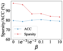
(a) Cora

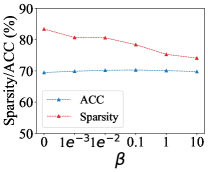
(b) Citeseer

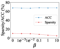
(c) Ogbn-arxiv

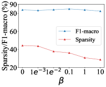
(d) Amazon

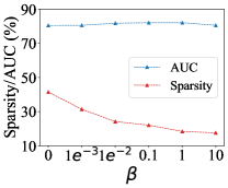
(e) DBLP

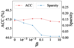
(f) Flickr

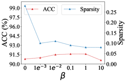
(g) Reddit

Figure 6: Evaluations of $\beta$ in seven datasets. For the Flickr and Reddit datasets, due to the datasets’ low sparsity, we use the shared x-axis form for the Flickr and Reddit figures.

C.6 More cross-architecture experiments

In this subsection, we further report the results of cross-architecture experiments on the YelpChi. As shown in Tab.  7, our SGDD  improves the performance in all cases, the average improvements compared to the GCond [35] is 9.6%, which indicates the strong generalization performance of the condensed graph by SGDD.

Table 7: Comparison of the cross-architecture generalization performance between GCond and SGDD on YelpChi. Bold entries are the best results. $\uparrow$/$\downarrow$: our method show increase or decrease performance.

C/T	APPNP	Cheby	GCN	SAGE	SGC
	GCond / SGDD	GCond / SGDD	GCond / SGDD	GCond / SGDD	GCond / SGDD
APPNP	48.1 / 55.1$\uparrow$	46.5 / 57.4$\uparrow$	50.1 / 58.6$\uparrow$	46.7 / 57.1$\uparrow$	49.6 / 57.6$\uparrow$
Cheby	48.0 / 56.2$\uparrow$	45.9 / 56.8$\uparrow$	49.8 / 58.7$\uparrow$	46.8 / 58.3$\uparrow$	49.8 / 58.4$\uparrow$
GCN	47.6 / 56.5$\uparrow$	46.6 / 56.8$\uparrow$	48.6 / 59.7$\uparrow$	47.4 / 57.6$\uparrow$	50.1 / 57.4$\uparrow$
SAGE	46.7 / 57.6$\uparrow$	46.8 / 57.5$\uparrow$	48.9 / 58.7$\uparrow$	48.6 / 58.6$\uparrow$	48.9 / 58.6$\uparrow$
SGC	47.6 / 57.6$\uparrow$	47.7 / 57.2$\uparrow$	48.6 / 57.8$\uparrow$	47.4 / 59.0$\uparrow$	48.7 / 57.6$\uparrow$

C.7 Ablation of the sampling operation in OT distance

To further reduce condensing time and memory usage, we follow GCond [35] to sample from original graph $\mathbf{A}$ in the condensing stage (line 11 in the Algorithm 1). We evaluate the SGDD  on various sample sizes, i.e., {100, 500, 1000, 2000, 5000}, and report the corresponding performance and $SC$. As shown in Fig. 7, with the increase in the number of nodes, the performance obtains marginal improvements while the $SC$ is decreasing. However, larger sample sizes are not always beneficial to performance. In this study, the highest results are obtained when the sample size is 2000. This result empirically demonstrates the scalability of the structure learning module. Specifically, the module enables efficient condensing on large graphs.

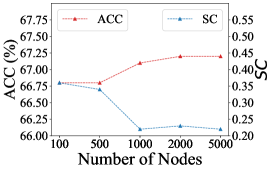
(a) Ogbn-arxiv

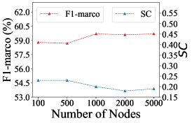
(b) YelpChi

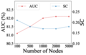
(c) DBLP

Figure 7: Evaluation of the number of sampled nodes to the performance.

C.8 More discussion of the condensed graphs.

We next show the comparison of condensed graphs and original graphs. As shown in Tab. 8, the condensed graphs obviously have fewer nodes and edges, while maintaining comparable accuracy, which shows the effectiveness of our SGDD . We also represent the visualizations of some condensed graphs. In Fig. 8, the black lines denote that edge weights are larger than 0.5 and the gray lines represent as smaller than 0.5. We can observe that there are some patterns in the condensed graph, e.g., the homophily patterns on Cora and Citeseer. However, for the remaining datasets, the visualizations are inadequate in revealing the properties of the condensed graph, which proves the superiority of analyzing structure in spectral view.

Table 8: The comparison between condensed graphs and original graphs.

	Citeseer, r=0.9%		Cora, r=1.3%		Ogbn-arxiv, r=0.5%		Flickr, r=0.1%		Reddit, r=0.1%
	Whole	SGDD	Whole	SGDD	Whole	SGDD	Whole	SGDD	Whole	SGDD
Accuracy	70.7	69.5	81.5	79.6	71.4	65.3	47.1	47.1	94.1	90.5
#Nodes	3k3	60	2k7	70	169k	454	44k	44	153k	153
#Edges	4k7	1k	5k4	2k	1,166k	8k6	218k	331	10,753k	3k
Storage(MB)	47.1	0.8	14.9	0.4	100.4	1.0	86.8	0.1	435.5	0.7

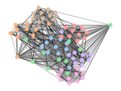
(a) Cora

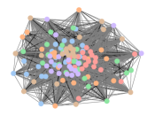
(b) Citeseer

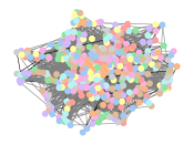
(c) Ogbn-arxiv

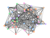
(d) Flickr

Figure 8: Visualizations of condensed graphs, the different colors on the graphs denote the classes.

References

- [1] Muhammet Balcilar, Guillaume Renton, Pierre Héroux, Benoit Gaüzère, Sébastien Adam, and Paul Honeine. Analyzing the expressive power of graph neural networks in a spectral perspective. In 9th International Conference on Learning Representations, ICLR 2021, Virtual Event, Austria, May 3-7, 2021, 2021.
- [2] Peter W Battaglia, Jessica B Hamrick, Victor Bapst, Alvaro Sanchez-Gonzalez, Vinicius Zambaldi, Mateusz Malinowski, Andrea Tacchetti, David Raposo, Adam Santoro, Ryan Faulkner, et al. Relational inductive biases, deep learning, and graph networks. ArXiv preprint, 2018.
- [3] Daniel Bear, Chaofei Fan, Damian Mrowca, Yunzhu Li, Seth Alter, Aran Nayebi, Jeremy Schwartz, Li Fei-Fei, Jiajun Wu, Josh Tenenbaum, and Daniel L. K. Yamins. Learning physical graph representations from visual scenes. In Advances in Neural Information Processing Systems 33: Annual Conference on Neural Information Processing Systems 2020, NeurIPS 2020, December 6-12, 2020, virtual, 2020.
- [4] Joan Bruna, Wojciech Zaremba, Arthur Szlam, and Yann LeCun. Spectral networks and locally connected networks on graphs. In 2nd International Conference on Learning Representations, ICLR 2014, Banff, AB, Canada, April 14-16, 2014, Conference Track Proceedings, 2014.
- [5] Chen Cai, Dingkang Wang, and Yusu Wang. Graph coarsening with neural networks. In 9th International Conference on Learning Representations, ICLR 2021, Virtual Event, Austria, May 3-7, 2021, 2021.
- [6] George Cazenavette, Tongzhou Wang, Antonio Torralba, Alexei A Efros, and Jun-Yan Zhu. Dataset distillation by matching training trajectories. In CVPR, 2022.
- [7] George Cazenavette, Tongzhou Wang, Antonio Torralba, Alexei A Efros, and Jun-Yan Zhu. Generalizing dataset distillation via deep generative prior. In Proceedings of the IEEE/CVF Conference on Computer Vision and Pattern Recognition, pages 3739–3748, 2023.
- [8] Yu Chen, Lingfei Wu, and Mohammed J. Zaki. Iterative deep graph learning for graph neural networks: Better and robust node embeddings. In Advances in Neural Information Processing Systems 33: Annual Conference on Neural Information Processing Systems 2020, NeurIPS 2020, December 6-12, 2020, virtual, 2020.
- [9] Marco Cuturi. Sinkhorn distances: Lightspeed computation of optimal transport. In NIPS, pages 2292–2300, 2013.
- [10] Évariste Daller, Sébastien Bougleux, Luc Brun, and Olivier Lézoray. Local patterns and supergraph for chemical graph classification with convolutional networks. In Structural, Syntactic, and Statistical Pattern Recognition - Joint IAPR International Workshop, S+SSPR 2018, Beijing, China, August 17-19, 2018, Proceedings, volume 11004, pages 97–106, 2018.
- [11] Tuan Van Dao, Hiroshi Sato, and Masao Kubo. Mlp-mixer-autoencoder: A lightweight ensemble architecture for malware classification. Inf., 14(3):167, 2023.
- [12] Kinkar Ch. Das, Seyed Ahmad Mojallal, and Vilmar Trevisan. Distribution of laplacian eigenvalues of graphs. Linear Algebra and its Applications, 508:48–61, 2016.
- [13] Michaël Defferrard, Xavier Bresson, and Pierre Vandergheynst. Convolutional neural networks on graphs with fast localized spectral filtering. In Advances in Neural Information Processing Systems 29: Annual Conference on Neural Information Processing Systems 2016, December 5-10, 2016, Barcelona, Spain, 2016.
- [14] Chenhui Deng, Zhiqiang Zhao, Yongyu Wang, Zhiru Zhang, and Zhuo Feng. Graphzoom: A multi-level spectral approach for accurate and scalable graph embedding. In 8th International Conference on Learning Representations, ICLR 2020, Addis Ababa, Ethiopia, April 26-30, 2020, 2020.
- [15] Holger Ebel and Stefan Bornholdt. Coevolutionary games on networks. Physical Review E, 66(5):056118, 2002.
- [16] Justin Eldridge, Mikhail Belkin, and Yusu Wang. Graphons, mergeons, and so on! Advances in Neural Information Processing Systems, 29, 2016.
- [17] Matthias Fey and JanEric Lenssen. Fast graph representation learning with pytorch geometric, Mar 2019.
- [18] Luca Franceschi, Mathias Niepert, Massimiliano Pontil, and Xiao He. Learning discrete structures for graph neural networks. In Proceedings of the 36th International Conference on Machine Learning, ICML 2019, 9-15 June 2019, Long Beach, California, USA, Proceedings of Machine Learning Research, 2019.
- [19] Alan Frieze and Ravi Kannan. Quick approximation to matrices and applications. Combinatorica, 19(2):175–220, 1999.
- [20] Shuang Gao and Peter E Caines. Graphon control of large-scale networks of linear systems. IEEE Transactions on Automatic Control, 2019.
- [21] Jiahui Geng, Zongxiong Chen, Yuandou Wang, Herbert Woisetschlaeger, Sonja Schimmler, Ruben Mayer, Zhiming Zhao, and Chunming Rong. A survey on dataset distillation: Approaches, applications and future directions. ArXiv, abs/2305.01975, 2023.
- [22] Jianyang Gu, Kai Wang, Wei Jiang, and Yang You. Summarizing stream data for memory-restricted online continual learning. arXiv preprint arXiv:2305.16645, 2023.
- [23] Ziyao Guo, Kai Wang, George Cazenavette, Hui Li, Kaipeng Zhang, and Yang You. Towards lossless dataset distillation via difficulty-aligned trajectory matching. arXiv preprint arXiv:2310.05773, 2023.
- [24] Ivan Gutman and Bo Zhou. Laplacian energy of a graph. Linear Algebra and its Applications, 414(1):29–37, 2006.
- [25] William L. Hamilton, Zhitao Ying, and Jure Leskovec. Inductive representation learning on large graphs. In NeurIPS, 2017.
- [26] Peter D Hoff, Adrian E Raftery, and Mark S Handcock. Latent space approaches to social network analysis. Journal of the american Statistical association, 97(460):1090–1098, 2002.
- [27] Paul W Holland, Kathryn Blackmond Laskey, and Samuel Leinhardt. Stochastic blockmodels: First steps. Social networks, 5(2):109–137, 1983.
- [28] Weihua Hu, Matthias Fey, Marinka Zitnik, Yuxiao Dong, Hongyu Ren, Bowen Liu, Michele Catasta, and Jure Leskovec. Open graph benchmark: Datasets for machine learning on graphs. In NeurIPS, 2020.
- [29] Zengfeng Huang, Shengzhong Zhang, Chong Xi, Tang Liu, and Min Zhou. Scaling up graph neural networks via graph coarsening. In In Proceedings of the 27th ACM SIGKDD Conference on Knowledge Discovery and Data Mining (KDD ’21), 2021.
- [30] Joseph J. Pfeiffer III, Sebastián Moreno, Timothy La Fond, Jennifer Neville, and Brian Gallagher. Attributed graph models: modeling network structure with correlated attributes. In WWW, 2014.
- [31] Svante Janson. Graphons, cut norm and distance, couplings and rearrangements. New York journal of mathematics, 2013.
- [32] Svante Janson and Persi Diaconis. Graph limits and exchangeable random graphs. Rendiconti di Matematica e delle sue Applicazioni. Serie VII, pages 33–61, 2008.
- [33] Wei Jin, Yao Ma, Xiaorui Liu, Xianfeng Tang, Suhang Wang, and Jiliang Tang. Graph structure learning for robust graph neural networks. In KDD, 2020.
- [34] Wei Jin, Xianfeng Tang, Haoming Jiang, Zheng Li, Danqing Zhang, Jiliang Tang, and Bing Yin. Condensing graphs via one-step gradient matching. In Proceedings of the 28th ACM SIGKDD Conference on Knowledge Discovery and Data Mining, Aug 2022.
- [35] Wei Jin, Lingxiao Zhao, Shichang Zhang, Yozen Liu, Jiliang Tang, and Neil Shah. Graph condensation for graph neural networks. In ICLR, 2022.
- [36] David R. Karger. Random sampling in cut, flow, and network design problems. Math. Oper. Res., 24(2):383–413, 1999.
- [37] Jang-Hyun Kim, Jinuk Kim, Seong Joon Oh, Sangdoo Yun, Hwanjun Song, Joonhyun Jeong, Jung-Woo Ha, and Hyun Oh Song. Dataset condensation via efficient synthetic-data parameterization. arXiv:2205.14959, 2022.
- [38] Thomas N. Kipf and Max Welling. Semi-supervised classification with graph convolutional networks. In 5th International Conference on Learning Representations, ICLR 2017, Toulon, France, April 24-26, 2017, Conference Track Proceedings. OpenReview.net, 2017.
- [39] Thomas N. Kipf and Max Welling. Semi-supervised classification with graph convolutional networks. In ICLR, 2017.
- [40] Johannes Klicpera, Aleksandar Bojchevski, and Stephan Günnemann. Predict then propagate: Graph neural networks meet personalized pagerank. In ICLR 2019, 2019.
- [41] Eric D. Kolaczyk. Statistical Analysis of Network Data: Methods and Models. Springer, 2009.
- [42] Saehyung Lee, Sanghyuk Chun, Sangwon Jung, Sangdoo Yun, and Sungroh Yoon. Dataset condensation with contrastive signals. In ICML, 2022.
- [43] Guanzhi Li, Aining Zhang, Qizhi Zhang, Di Wu, and Choujun Zhan. Pearson correlation coefficient-based performance enhancement of broad learning system for stock price prediction. IEEE Trans. Circuits Syst. II Express Briefs, 69(5):2413–2417, 2022.
- [44] Jianxin Li, Qingyun Sun, Hao Peng, Beining Yang, Jia Wu, and S Yu Phillp. Adaptive subgraph neural network with reinforced critical structure mining. IEEE Transactions on Pattern Analysis and Machine Intelligence, 2023.
- [45] Jianhua Lin. Divergence measures based on the shannon entropy. IEEE Trans. Inf. Theory, 37(1):145–151, 1991.
- [46] Zhiqi Lin, Cheng Li, Youshan Miao, Yunxin Liu, and Yinlong Xu. Pagraph: Scaling gnn training on large graphs via computation-aware caching. In Proceedings of the 11th ACM Symposium on Cloud Computing, Oct 2020.
- [47] Hanxiao Liu, Karen Simonyan, and Yiming Yang. DARTS: differentiable architecture search. In ICLR, 2019.
- [48] Mengyang Liu, Shanchuan Li, Xinshi Chen, and Le Song. Graph condensation via receptive field distribution matching. arXiv preprint arXiv:2206.13697, 2022.
- [49] Yanqing Liu, Jianyang Gu, Kai Wang, Zheng Zhu, Wei Jiang, and Yang You. Dream: Efficient dataset distillation by representative matching. arXiv preprint arXiv:2302.14416, 2023.
- [50] Andreas Loukas. Graph reduction with spectral and cut guarantees. J. Mach. Learn. Res., 20:116:1–116:42, 2019.
- [51] Andreas Loukas and Pierre Vandergheynst. Spectrally approximating large graphs with smaller graphs. In Proceedings of the 35th International Conference on Machine Learning, ICML 2018, Stockholmsmässan, Stockholm, Sweden, July 10-15, 2018, Proceedings of Machine Learning Research, 2018.
- [52] László Lovász. Large networks and graph limits, volume 60. American Mathematical Soc., 2012.
- [53] Dongsheng Luo, Wei Cheng, Wenchao Yu, Bo Zong, Jingchao Ni, Haifeng Chen, and Xiang Zhang. Learning to drop: Robust graph neural network via topological denoising. In WSDM, pages 779–787, 2021.
- [54] Hermina Petric Maretic, Mireille El Gheche, Giovanni Chierchia, and Pascal Frossard. Got: An optimal transport framework for graph comparison. In NeurIPS, 2019.
- [55] Brendan D. McKay, Mehmet Aziz Yirik, and Christoph Steinbeck. Surge: a fast open-source chemical graph generator. J. Cheminformatics, 2022.
- [56] Facundo Mémoli. Spectral Gromov-Wasserstein distances for shape matching. In ICCV Workshops, pages 256–263, 2009.
- [57] Matthew W. Morency and Geert Leus. Graphon filters: Graph signal processing in the limit. IEEE Trans. Signal Process., 69:1740–1754, 2021.
- [58] Bilal Nehme, Olivier Strauss, and Kevin Loquin. Estimating the variance of a kernel density estimation. In Christian Borgelt, Gil González-Rodríguez, Wolfgang Trutschnig, María Asunción Lubiano, María Ángeles Gil, Przemyslaw Grzegorzewski, and Olgierd Hryniewicz, editors, Combining Soft Computing and Statistical Methods in Data Analysis, SMPS 2010, Oviedo, Spain, September 29 - October 1, 2010, volume 77 of Advances in Intelligent and Soft Computing, pages 483–490. Springer, 2010.
- [59] Timothy Nguyen, Zhourong Chen, and Jaehoon Lee. Dataset meta-learning from kernel ridge-regression. In ICLR, 2021.
- [60] Timothy Nguyen, Roman Novak, Lechao Xiao, and Jaehoon Lee. Dataset distillation with infinitely wide convolutional networks. NeurIPS, 34, 2021.
- [61] Shirui Pan, Ruiqi Hu, Guodong Long, Jing Jiang, Lina Yao, and Chengqi Zhang. Adversarially regularized graph autoencoder for graph embedding. In Proceedings of the Twenty-Seventh International Joint Conference on Artificial Intelligence, IJCAI 2018, July 13-19, 2018, Stockholm, Sweden, 2018.
- [62] Francesca Parise and Asuman Ozdaglar. Graphon games: A statistical framework for network games and interventions. arXiv preprint arXiv:1802.00080, 2018.
- [63] Adam Paszke, Sam Gross, Francisco Massa, Adam Lerer, James Bradbury, Gregory Chanan, Trevor Killeen, Zeming Lin, Natalia Gimelshein, Luca Antiga, et al. Pytorch: An imperative style, high-performance deep learning library. Advances in neural information processing systems, 32, 2019.
- [64] David Peleg and Alejandro A. Schäffer. Graph spanners. J. Graph Theory, 13(1):99–116, 1989.
- [65] Bryan Perozzi, Rami Al-Rfou, and Steven Skiena. Deepwalk: online learning of social representations. In The 20th ACM SIGKDD International Conference on Knowledge Discovery and Data Mining, KDD ’14, New York, NY, USA - August 24 - 27, 2014, 2014.
- [66] Shebuti Rayana and Leman Akoglu. Collective opinion spam detection: Bridging review networks and metadata. In Proceedings of the 21th ACM SIGKDD International Conference on Knowledge Discovery and Data Mining, KDD ’15, page 985–994, New York, NY, USA, 2015. Association for Computing Machinery.
- [67] Luana Ruiz, Luiz Chamon, and Alejandro Ribeiro. Graphon neural networks and the transferability of graph neural networks. Advances in Neural Information Processing Systems, 33:1702–1712, 2020.
- [68] Luana Ruiz, Luiz F. O. Chamon, and Alejandro Ribeiro. The graphon fourier transform. In ICASSP, 2020.
- [69] Luana Ruiz, Luiz FO Chamon, and Alejandro Ribeiro. Graphon signal processing. IEEE Transactions on Signal Processing, 69:4961–4976, 2021.
- [70] Ozan Sener and Silvio Savarese. Active learning for convolutional neural networks: A core-set approach. In ICLR, 2018.
- [71] Cosma Rohilla Shalizi and Andrew C. Thomas. Homophily and contagion are generically confounded in observational social network studies. CoRR, abs/1004.4704, 2010.
- [72] Chao Shang, Jie Chen, and Jinbo Bi. Discrete graph structure learning for forecasting multiple time series. In International Conference on Learning Representations, 2021.
- [73] Mingjia Shi, Yuhao Zhou, Kai Wang, Huaizheng Zhang, Shudong Huang, Qing Ye, and Jiancheng Lv. PRIOR: Personalized prior for reactivating the information overlooked in federated learning. In Proceedings of the 37th NeurIPS, 2023.
- [74] Vincent Sitzmann, Julien N. P. Martel, Alexander W. Bergman, David B. Lindell, and Gordon Wetzstein. Implicit neural representations with periodic activation functions. In NeurIPS, 2020.
- [75] Daniel A. Spielman and Nikhil Srivastava. Graph sparsification by effective resistances. SIAM J. Comput., 40(6):1913–1926, 2011.
- [76] Daniel A. Spielman and Shang-Hua Teng. Spectral sparsification of graphs. SIAM J. Comput., 40(4):981–1025, 2011.
- [77] Qingyun Sun, Jianxin Li, Hao Peng, Jia Wu, Xingcheng Fu, Cheng Ji, and S Yu Philip. Graph structure learning with variational information bottleneck. In AAAI, volume 36, pages 4165–4174, 2022.
- [78] Qingyun Sun, Jianxin Li, Hao Peng, Jia Wu, Yuanxing Ning, Philip S Yu, and Lifang He. Sugar: Subgraph neural network with reinforcement pooling and self-supervised mutual information mechanism. In WWW 2021, pages 2081–2091, 2021.
- [79] Qingyun Sun, Jianxin Li, Haonan Yuan, Xingcheng Fu, Hao Peng, Cheng Ji, Qian Li, and Philip S Yu. Position-aware structure learning for graph topology-imbalance by relieving under-reaching and over-squashing. In CIKM, pages 1848–1857, 2022.
- [80] Jianheng Tang, Jiajin Li, Ziqi Gao, and Jia Li. Rethinking graph neural networks for anomaly detection. In ICML, May 2022.
- [81] Jie Tang, Jing Zhang, Limin Yao, Juanzi Li, Li Zhang, and Zhong Su. Arnetminer: Extraction and mining of academic social networks. In Proceedings of the 14th ACM SIGKDD International Conference on Knowledge Discovery and Data Mining, KDD ’08, page 990–998, New York, NY, USA, 2008. Association for Computing Machinery.
- [82] Petar Velickovic, Guillem Cucurull, Arantxa Casanova, Adriana Romero, Pietro Liò, and Yoshua Bengio. Graph attention networks. In ICLR, 2018.
- [83] Renato Vizuete, Federica Garin, and Paolo Frasca. The laplacian spectrum of large graphs sampled from graphons. IEEE Transactions on Network Science and Engineering, page 1711–1721, Mar 2021.
- [84] Kai Wang, Jianyang Gu, Daquan Zhou, Zheng Zhu, Wei Jiang, and Yang You. Dim: Distilling dataset into generative model. arXiv preprint arXiv:2303.04707, 2023.
- [85] Kai Wang, Bo Zhao, Xiangyu Peng, Zheng Zhu, Shuo Yang, Shuo Wang, Guan Huang, Hakan Bilen, Xinchao Wang, and Yang You. Cafe: Learning to condense dataset by aligning features. In CVPR, 2022.
- [86] Tongzhou Wang, Jun-Yan Zhu, Antonio Torralba, and Alexei A Efros. Dataset distillation. ArXiv preprint, 2018.
- [87] Yili Wang, Kaixiong Zhou, Rui Miao, Ninghao Liu, and Xin Wang. Adagcl: Adaptive subgraph contrastive learning to generalize large-scale graph training.
- [88] Max Welling. Herding dynamical weights to learn. In ICML, 2009.
- [89] Gert W. Wolf. Facility location: concepts, models, algorithms and case studies. series: Contributions to management science. Int. J. Geogr. Inf. Sci., 25(2):331–333, 2011.
- [90] Felix Wu, Amauri H. Souza Jr., Tianyi Zhang, Christopher Fifty, Tao Yu, and Kilian Q. Weinberger. Simplifying graph convolutional networks. In ICML, 2019.
- [91] Zonghan Wu, Shirui Pan, Fengwen Chen, Guodong Long, Chengqi Zhang, and Philip S Yu. A comprehensive survey on graph neural networks. ArXiv preprint, 2019.
- [92] Xinyue Xia, Gal Mishne, and Yusu Wang. Implicit graphon neural representation. In Proceedings of the 26th International Conference on Artificial Intelligence and Statistics, AISTATS, Nov 2023.
- [93] Hongteng Xu, Dixin Luo, Lawrence Carin, and Hongyuan Zha. Learning graphons via structured Gromov-Wasserstein barycenters. In Proceedings of the AAAI Conference on Artificial Intelligence, volume 35, pages 10505–10513, 2021.
- [94] Shuo Yang, Zeke Xie, Hanyu Peng, Min Xu, Mingming Sun, and Ping Li. Dataset pruning: Reducing training data by examining generalization influence. arXiv preprint arXiv:2205.09329, 2022.
- [95] Zhilin Yang, William W. Cohen, and Ruslan Salakhutdinov. Revisiting semi-supervised learning with graph embeddings. In ICML, JMLR Workshop and Conference Proceedings, 2016.
- [96] W. Sawin Yihe Dong. Copt: Coordinated optimal transport on graphs. In 34th Conference on Neural Information Processing Systems, Vancouver, Canada, 2020.
- [97] Rex Ying, Ruining He, Kaifeng Chen, Pong Eksombatchai, William L. Hamilton, and Jure Leskovec. Graph convolutional neural networks for web-scale recommender systems. In KDD, 2018.
- [98] Haiyang Yu, Limei Wang, Bokun Wang, Meng Liu, Tianbao Yang, and Shuiwang Ji. Graphfm: Improving large-scale gnn training via feature momentum. In ICML, Jun 2022.
- [99] Hanqing Zeng, Hongkuan Zhou, Ajitesh Srivastava, Rajgopal Kannan, and Viktor K. Prasanna. Graphsaint: Graph sampling based inductive learning method. In ICLR, 2020.
- [100] Muhan Zhang and Yixin Chen. Link prediction based on graph neural networks. In Samy Bengio, Hanna M. Wallach, Hugo Larochelle, Kristen Grauman, Nicolò Cesa-Bianchi, and Roman Garnett, editors, NeurIPS, pages 5171–5181, 2018.
- [101] Shijie Zhang, Hongzhi Yin, Tong Chen, Quoc Viet Hung Nguyen, Zi Huang, and Lizhen Cui. Gcn-based user representation learning for unifying robust recommendation and fraudster detection. In SIGIR, pages 689–698. ACM, 2020.
- [102] Yifan Zhang, Daquan Zhou, Bryan Hooi, Kai Wang, and Jiashi Feng. Expanding small-scale datasets with guided imagination. arXiv preprint arXiv:2211.13976, 2022.
- [103] Bo Zhao and Hakan Bilen. Dataset condensation with distribution matching. arXiv preprint arXiv:2110.04181, 2021.
- [104] Bo Zhao, Konda Reddy Mopuri, and Hakan Bilen. Dataset condensation with gradient matching. In ICLR, 2021.
- [105] Bo Zhao, Konda Reddy Mopuri, and Hakan Bilen. Dataset condensation with gradient matching. In Ninth International Conference on Learning Representations 2021, 2021.
- [106] Tong Zhao, Yozen Liu, Leonardo Neves, Oliver Woodford, Meng Jiang, and Neil Shah. Data augmentation for graph neural networks. In AAAI, 2021.
- [107] Cheng Zheng, Bo Zong, Wei Cheng, Dongjin Song, Jingchao Ni, Wenchao Yu, Haifeng Chen, and Wei Wang. Robust graph representation learning via neural sparsification. In ICML, pages 11458–11468, 2020.
- [108] Daquan Zhou, Kai Wang, Jianyang Gu, Xiangyu Peng, Dongze Lian, Yifan Zhang, Yang You, and Jiashi Feng. Dataset quantization. In Proceedings of the IEEE/CVF International Conference on Computer Vision, pages 17205–17216, 2023.
- [109] Jie Zhou, Ganqu Cui, Zhengyan Zhang, Cheng Yang, Zhiyuan Liu, Lifeng Wang, Changcheng Li, and Maosong Sun. Graph neural networks: A review of methods and applications. ArXiv preprint, 2018.