Adiabatic perturbation theory for two-component systems with one heavy component

Abstract

A systematic adiabatic perturbation theory with respect to the kinetic energy of the heavy component of a two-component quantum system is introduced. The effective Schrödinger equation for the heavy system is derived to second order in the inverse mass. It contains a new form of kinetic energy operator with a Hermitian mass tensor and a complex-valued vector potential. All of the potentials in the effective equation can be computed without having to evaluate sums over the eigenstates of the light system. The most salient potential application of the theory is to systems of electrons and nuclei. The accuracy of the theory is verified numerically in a model of a diatomic molecule and analytically in a linear vibronic model.

I Introduction

Perturbation theory with respect to a potential perturbation is very well established, providing successively higher order approximations to an eigenfunction of the Schrödinger equation. In a two-component system with one component that is much heavier than the other, it makes sense to seek a perturbation theory with respect to the kinetic energy of the heavy component. Such a perturbation theory should yield a sequence of approximations that are accurate to successively higher, usually fractional, powers of $M^{-1}$, where $M$ is the mass of the heavy component. The two components could be two different species of particles, such as electrons and nuclei, or two different types of degrees of freedom if one type is effectively heavier than the other.

Born and Oppenheimer Born and Oppenheimer (1927) and Slater Slater (1927) proposed an adiabatic approximation in which the electronic wavefunction is taken to be an eigenstate of the Hamiltonian with the nuclear coordinates held fixed. The corresponding nuclear coordinate-dependent eigenvalue acts as a potential in an effective Schrödinger equation for the nuclei. Solving that effective nuclear Schrödinger equation provides a crude adiabatic approximation. Born and Oppenheimer introduced a method for improving upon this adiabatic approximation by developing a perturbation series in powers of $(m/M)^{1/4}$. Unfortunately, it is impractical to apply in general because it requires the evaluation of infinite sums over the eigenstates of the adiabatic Hamiltonian. No systematic quantum perturbation theory for the $M\rightarrow\infty$ limit that avoids these summations has been found. This is the problem that is solved in this paper.

Our strategy is to perform a sequence of near-identity unitary transformations to decouple a nondegenerate eigenstate of interest from all other states to a given order in $M^{-1}$. The most important antecedents to our theory are Littlejohn and Weigert’s pioneering development of near-identity transformations to diagonalize a coupled-wave Hamiltonian order-by-order in powers of $\hbar$ in the semiclassical limit Littlejohn and Weigert (1993); Weigert and Littlejohn (1993) and Mead and Truhlar’s discovery of effective magnetic gauge potentials in the nuclear Schrödinger equation of a molecule Mead and Truhlar (1979).

Nonadiabatic corrections to the crude adiabatic approximation described above are important in a wide range of problems in condensed matter physics and molecular physics. However, unless two potentials – the Mead-Truhlar vector potential and a geometric scalar potential – are added to the crude nuclear Schrödinger equation, the energy eigenvalue is not accurate to order $M^{-1}$. These two potentials are not usually included. There is growing interest in nonadiabatic effects in electron-phonon systems Ferrari (2007); Basko et al. (2009); Dean et al. (2010); De Fillipis et al. (2010); Klimin et al. (2016); Ponosov and Streltsov (2016, 2017); Lazzeri and Mauri (2006); Bock et al. (2006); Pisana et al. (2007); Piscanec et al. (2007); Calandra et al. (2007); Caudal et al. (2007); Saitta et al. (2008); Calandra et al. (2010); Gonze et al. (2011); Cannuccia and Marini (2012); Marini et al. (2015); Poncé et al. (2015); Antonius et al. (2015); M. d’Astuto et al. (2016); Gali et al. (2016); Nery and Allen (2016); Allen and Nery (2017); Giustino (2017); Long and Prezhdo (2017); Zhou et al. (2017); Caruso et al. (2017); Nery et al. (2018); Marini and Pavlyukh (2018); Novko (2018); Requist et al. (2019); Pellegrini et al. (2022); Talantsev (2023); Girotto and Novko (2023); Brousseau-Couture et al. (2023) and molecules Makhov et al. (2014); Min et al. (2015); Requist et al. (2016); Requist and Gross (2016); Li et al. (2018); Crespo-Otero and Barbatti (2018); Loncarić et al. (2019); Agostini and Curchod (2019); Martinazzo and Burghardt (2022); Villaseco Arribas et al. (2022); Kocák et al. (2023); Manfredi et al. (2023); Gardner et al. (2023); Bombín et al. (2023); Athavale et al. (2021).

The nonrelativistic Hamiltonian of a two-component system is

$$\mathcal{H} =H(x)-\frac{\epsilon}{2}\frac{1}{\sqrt{g_{0}}}\partial_{\mu}\big{(}\sqrt{g_{0}}g_{0}^{\mu\nu}\partial_{\nu}\big{)}{,}$$ (1)

where $x=\{x^{\mu}\}$ denotes the generalized, possibly curvilinear, coordinates of the heavy particles. The first term is the adiabatic Hamiltonian, which includes the light component kinetic energy and all potentials, and the second term is the heavy component kinetic energy containing the Laplace-Beltrami operator, a coordinate-invariant operator expressed in terms of an $x$-dependent metric $g_{0\mu\nu}$; we use the summation convention. The small parameter $\epsilon$ is

$$\epsilon=\frac{\frac{\hbar^{2}}{ML^{2}}}{\Delta}{,}$$ (2)

where $\hbar^{2}/ML^{2}$ is an energy scale for the nuclear kinetic energy and $\Delta$ is an energy scale for the light system, e.g. a characteristic energy gap of $H$; $L$ is a characteristic length and $M$ is a characteristic mass. This definition is useful when the light system is modeled by a Hamiltonian that does not explicitly contain a light mass $m$. However, it includes the more common definition $\epsilon=m/M$ as a special case, as we are free to choose $L$ and $\Delta$ such that $\hbar^{2}/\Delta L^{2}$ equals $m$. Eq. (1) is given in the energy units $\Delta$.

II Results

Our main result is the derivation of the following second-order effective Schrödinger equation for the wave function $\zeta_{n}$ of the heavy component given that the light system predominantly occupies the state $|n\rangle$:

$$-\frac{\epsilon}{2}\frac{1}{\sqrt{g_{0}}}\big{(}\partial_{\mu}-iA^{(2)*}_{\mu}\big{)}\sqrt{g_{0}}h^{(2)\mu\nu}\big{(}\partial_{\nu}-iA^{(2)}_{\nu}\big{)}\zeta_{n}+E_{n}\zeta_{n}+\epsilon V_{geo}\zeta_{n}+\epsilon^{2}V_{2,geo}\zeta_{n}=\lambda_{n}\zeta_{n}{.}$$ (3)

The formulas for all quantities are given below; $h^{(2)\mu\nu}$ is a Hermitian inverse effective mass tensor, $A_{\nu}^{(2)}$ is a complex-valued effective gauge potential, $E_{n}$ is the $x$-dependent eigenvalue of the adiabatic Hamiltonian $H=H(x)$, and $V_{geo}$ and $V_{2,geo}$ are effective potentials. Equation (3) is gauge- and coordinate-invariant and contains a new form of Hermitian kinetic energy operator.

Our strategy is influenced by Littlejohn and Weigert’s calculations Littlejohn and Weigert (1993); Weigert and Littlejohn (1993), in which near-identity transformations were used to diagonalize a molecular or coupled-wave Hamiltonian to successively higher powers of $\hbar$. The eigenvalue equation

$$H|n\rangle=E_{n}|n\rangle$$ (4)

defines an $x$-dependent adiabatic basis $\{|n\rangle\}$. A general state of the two-component system can be expanded in the adiabatic basis as $|\psi\rangle=\sum_{n}|n\rangle\zeta_{n}$. We look for a near-identity unitary operator

$$U_{1}=e^{i\epsilon G_{1}(x,p)}$$ (5)

that transforms the adiabatic basis $\{|n\rangle\}$ to an improved adiabatic basis $\{|n^{(1)}\rangle\}$ in which the coefficient of the $n$th state $\zeta_{n}^{(1)}$ is decoupled from all other states to second order in $\epsilon$, i.e.

$$\mathcal{H}^{(1)}_{ln} =\langle l^{(1)}|U_{1}^{{\dagger}}\mathcal{H}U_{1}|n^{(1)}\rangle$$

$$=\mathcal{O}(\epsilon^{2})\hskip 71.13188pt\mathrm{for}\quad l\neq n{.}$$ (6)

Using the Baker-Campbell-Hausdorff formula to expand the transformed Hamiltonian in powers of $\epsilon$, we obtain the first-order effective Hamiltonian

$$\mathcal{H}^{\rm eff(1)}=H+\epsilon T-i\epsilon[G_{1},H]{.}$$ (7)

The condition in Eq. (6) will be satisfied if $G_{1}$ satisfies

$$\langle l|[G_{1},H]|n\rangle=-i\langle l|T|n\rangle\quad\mathrm{for}\;\mathrm{all}\;l\neq n{.}$$ (8)

Once we have found a suitable $G_{1}$, the coupling to other states will be order $\epsilon^{2}$ and therefore negligible when we are working to first order in $\epsilon$. Thus, the Hamiltonian to be used in the first-order effective Schrödinger equation is the diagonal element $\mathcal{H}^{\rm eff(1)}_{nn}=E_{n}+\epsilon T_{nn}$. Equation (8) does not determine the diagonal elements of $G_{1}$, which we choose to be zero. The first-order effective Schrödinger equation can be written in a gauge- and coordinate-invariant form as

$$-\frac{\epsilon}{2}\frac{1}{\sqrt{g_{0}}}\big{(}\partial_{\mu}-iA_{\mu}\big{)}\sqrt{g_{0}}g_{0}^{\mu\nu}\big{(}\partial_{\nu}-iA_{\nu}\big{)}\zeta_{n}^{(1)}+E_{n}\zeta_{n}^{(1)}+\epsilon V_{geo}\zeta_{n}^{(1)}=\lambda_{n}^{(1)}\zeta_{n}^{(1)}{,}$$ (9)

where $A_{\nu}=i\langle n|\partial_{\nu}n\rangle$ is the Mead-Truhlar-Berry gauge potential Mead and Truhlar (1979); Mead (1980); Berry (1984) and $V_{geo}$ is the first-order geometric scalar potential

$$V_{geo} =\frac{1}{2}g_{0}^{\mu\nu}\sum_{l\neq n}A_{\mu,nl}A_{\nu,ln}$$

$$=\frac{1}{2}g_{0}^{\mu\nu}\mathrm{Re}\langle D_{\mu}n|D_{\nu}n\rangle{,}$$ (10)

and $D_{\mu}=\partial_{\mu}+iA_{\mu}$ is the gauge-covariant derivative acting on $|n\rangle$. All of the potentials in Eq. (9) have been expressed in terms of $|n\rangle$ and its covariant derivatives. In particular, sums over adiabatic eigenstates have been eliminated, so there are no off-diagonal quantities such as $A_{\nu,ln}=i\langle l|\partial_{\nu}n\rangle$. The potentials have geometric significance. For example, the potential $V_{geo}$ was shown to be expressible in terms of the Provost-Vallee metric Provost and Vallee (1980), $g_{\mu\nu}=\mathrm{Re}\langle D_{\mu}n|D_{\nu}n\rangle$, by Berry Berry (1989) and further studied by Berry and Lim Berry and Lim (1990). An effective equation equivalent to Eq. (9) has been derived in the special case of an $x$-independent metric $g_{0\mu\nu}$ Berry (1989).

We now proceed to second order and look for a further unitary transformation $U_{2}=e^{i\epsilon^{2}G_{2}}$ which decouples the $n$th state to order $\epsilon^{3}$. The second-order effective Hamiltonian is

$$\mathcal{H}^{\rm eff(2)}=H+\epsilon T-i\epsilon[G_{1},H]-i\frac{\epsilon^{2}}{2}[G_{1},T]-i\epsilon^{2}[G_{2},H]{.}$$ (11)

To evaluate $\mathcal{H}^{\rm eff(2)}_{nn}$, we need to solve for $G_{1}$ and evaluate the commutator $[G_{1},T]$. Since $T$ is a second-order differential operator, we look for a solution to Eq. (8) of the form

$$G_{1,ln}=-\frac{1}{\sqrt{g_{0}}}\sum_{m}(\partial_{\mu}\delta_{lm}-iA_{\mu,lm})\sqrt{W_{ln}}W_{ln}^{\mu\nu}(\partial_{\nu}\delta_{mn}-iA_{\nu,mn})+U_{ln}{,}$$ (12)

where $W_{ln}=\det(W_{ln}^{\mu\nu})$. $G_{1}$ acts as a Hermitian operator on the vector $(\zeta_{1}^{(1)},\zeta_{2}^{(1)},\ldots)^{T}$ if $W_{ln}^{\mu\nu}=W_{nl}^{\nu\mu*}$ and $U_{ln}=U_{nl}^{*}$. $G_{1}$ will satisfy Eq. (8) if we choose

$$\sqrt{W_{ln}}W_{ln}^{\mu\nu}=\frac{i}{2}(E_{l}-E_{n})^{-1}\sqrt{g_{0}}g_{0}^{\mu\nu}$$ (13)

and

$$U_{ln}=-\frac{1}{2}(E_{l}-E_{n})^{-2}g_{0}^{\mu\nu}\partial_{\mu}(E_{l}+E_{n})A_{\nu,ln}{.}$$ (14)

Our $G_{1}$ differs from that of Littlejohn and Weigert Littlejohn and Weigert (1993) (see also Teufel (2003)), who treat a different limit.

The second-order effective Schrödinger equation in Eq. (3) can be derived by making the energy

$$\lambda_{n}^{(2)}=\frac{\epsilon}{2}\int\sqrt{g_{0}}D_{\nu}\zeta_{n}^{(2)*}g_{0}^{\nu\sigma}D_{\sigma}\zeta_{n}^{(2)}dx+\int\sqrt{g_{0}}(E_{n}+\epsilon V_{geo})|\zeta_{n}^{(2)}|^{2}dx+\epsilon^{2}\lambda_{2n}$$ (15)

stationary with respect to variations of $\zeta_{n}^{(2)}$; note that the superscript on $\zeta_{n}^{(2)}$ was suppressed in Eq. (3). The second-order contribution is

$$\lambda_{2n} =-\frac{i}{2}\int\sqrt{g_{0}}G_{1}\big{(}\zeta_{n}^{(2)*}\langle n^{(2)}|\big{)}T\big{(}|n^{(2)}\rangle\zeta_{n}^{(2)}\big{)}dx$$

$$\quad+\frac{i}{2}\int\sqrt{g_{0}}T\big{(}\zeta_{n}^{(2)*}\langle n^{(2)}|\big{)}G_{1}\big{(}|n^{(2)}\rangle\zeta_{n}^{(2)}\big{)}dx{.}$$ (16)

In the Euler-Lagrange equation, $\lambda_{2n}$ generates on the order of 225 terms containing inner products such as $\langle l|\partial_{\mu}H|m\rangle$. Remarkably, all of these terms are absorbed into the complex-valued gauge potential $A_{\mu}^{(2)}=A_{\mu}+\epsilon A_{2\mu}$, the effective mass tensor $h^{(2)}_{\mu\nu}=g_{0\mu\nu}+\epsilon h_{2\mu\nu}$, and the effective potential $V_{2,geo}$, which are given by the following compact formulas:

$$A_{2\nu} =\langle D_{\nu}n|(E_{n}-H)^{-1}|g_{0}^{\rho\sigma}\nabla^{(0)}_{\rho}\nabla^{(0)}_{\sigma}n\rangle-\langle D_{\nu}n|(E_{n}-H)^{-2}|D_{\rho}n\rangle g_{0}^{\rho\sigma}\partial_{\sigma}E_{n}$$ (17)

$$h_{2\mu\nu}=-2\langle D_{\mu}n|(E_{n}-H)^{-1}|D_{\nu}n\rangle$$ (18)

$$V_{2,geo} =+\frac{1}{4}\langle g_{0}^{\mu\nu}\nabla^{(0)}_{\mu}\nabla^{(0)}_{\nu}n|(E_{n}-H)^{-1}|g_{0}^{\rho\sigma}\nabla^{(0)}_{\rho}\nabla^{(0)}_{\sigma}n\rangle$$

$$\quad-\frac{1}{2}g_{0}^{\mu\nu}\partial_{\nu}E_{n}\mathrm{Re}\langle D_{\mu}n|(E_{n}-H)^{-2}|g_{0}^{\rho\sigma}\nabla^{(0)}_{\rho}\nabla^{(0)}_{\sigma}n\rangle{.}$$ (19)

Here we have introduced the covariant derivative $\nabla^{(0)}_{\mu}$ for which

$$\nabla^{(0)}_{\rho}\nabla^{(0)}_{\sigma}=D_{\rho}D_{\sigma}-\Gamma_{0\rho\sigma}^{\tau}D_{\tau}{,}$$ (20)

where $\Gamma_{0\mu\nu}^{\lambda}$ is the Christoffel symbol associated with $g_{0\mu\nu}$. Significantly, all of the potentials have been written in terms of the resolvent $(E_{n}-H)^{-1}$, $E_{n}$, $|n\rangle$, and covariant derivatives of $|n\rangle$, i.e. sums over adiabatic eigenstates have been eliminated, as in the first-order equation. The second-order correction $A_{2\nu}$ is manifestly gauge invariant. Hence the quantity $A_{\nu}^{(2)*}=A_{\nu}+\epsilon A_{2\nu}^{*}$ that appears in Eq. (3) transforms in exactly the same way as $A_{\nu}$ under the gauge transformation $|n\rangle\rightarrow e^{i\lambda}|n\rangle$, i.e. $A_{\nu}^{(2)*}\rightarrow A_{\nu}^{(2)*}-\partial_{\nu}\lambda$. The effective kinetic energy operator can be alternatively expressed as $-(\epsilon/2)h^{(2)\mu\nu}\hat{\nabla}_{\mu}^{(2)}\hat{\nabla}_{\nu}^{(2)}=-(\epsilon/2)h^{(2)\mu\nu}D_{\mu}D_{\nu}+(\epsilon/2)h^{(2)\mu\nu}\Lambda_{\mu\nu}^{(2)\lambda}D_{\lambda}$, where $\hat{\nabla}^{(2)}$ is a quantum covariant derivative with the symbol $\Lambda_{\mu\nu}^{(2)\lambda}$, similar to the one introduced in Ref. Requist (2023). Details of the calculations will be presented in a separate publication.

The above procedure can be carried out to arbitrary order in $\epsilon$. Solving the $p$th-order effective Schrödinger equation for the amplitude $\zeta_{n}^{(p)}$ allows us to calculate the energy eigenvalue with an accuracy of order $\epsilon^{p}$. Our theory also produces an approximation to the wave function of the full two-component system, which can be used to evaluate observables depending on the coordinates and momenta of the light component. To obtain the full wave function $|\psi\rangle$ of the two-component system, we first introduce a complete basis $\{|b\rangle\}$ for the $x$-space and write

$$|\psi^{(1)}\rangle =\sum_{nb}|n^{(1)}\rangle|b\rangle c_{nb}^{(1)}{,}$$ (21)

where $c_{nb}^{(1)}$ are constant coefficients. Our assumption that $|\psi\rangle$ predominantly occupies one adiabatic eigenstate $|n\rangle$ means that our approximation $|\psi^{(1)}\rangle=\sum_{k}|k^{(1)}\rangle\zeta_{k}^{(1)}$ contains only the $n$th element, i.e. $\zeta_{k}^{(1)}=0$ except if $k=n$. The corresponding expansion in the adiabatic basis is $|\psi\rangle=\sum_{ns}|n\rangle|b\rangle c_{nb}$. Then, we have

$$|\psi\rangle =U_{1}|\psi^{(1)}\rangle$$

$$=\sum_{b}|n\rangle|b\rangle c_{nb}^{(1)}+i\epsilon\sum_{mab}|m\rangle|a\rangle G_{1,ma,nb}c_{nb}^{(1)}+\mathcal{O}(\epsilon^{2}){.}$$ (22)

The procedure outlined above can be extended to arbitrary order, and at each order the potentials can be expressed in terms of the resolvent, $E_{n}$, $|n\rangle$, and its covariant derivatives. This is analogous to what was found in the adiabatic perturbation theory for explicitly time dependent Hamiltonians developed in Ref. Requist (2023), which can be viewed as a perturbation theory in the first-order differential operator $i\epsilon d/dt$.

In the original Hamiltonian of Eq. (1), we have not expressed the kinetic energy operator in a form in which the angular momentum operator appears explicitly, as would be required to make use of angular momentum quantum numbers. If this is needed, the gauge invariance of the equations with respect to the choice of a body-fixed frame can be maintained with the help of the formalism in Ref. Littlejohn and Reinsch (1997).

We now turn to the verification of adiabatic perturbation theory in two specific systems. The first is a two-state model of a diatomic molecule with the Hamiltonian

$$\mathcal{H} =-\frac{\hbar^{2}}{2M}\frac{d^{2}}{dx^{2}}+\left(\begin{array}[]{cc}D_{e}(1-e^{-a(x-x_{0})})^{2}&-c\\ -c&-\Delta+\frac{b}{x^{4}}\end{array}\right)$$ (25)

where the $(1,1)$ element of the matrix is the Morse potential. The adiabatic energies $E_{0}(x)$ and $E_{1}(x)$ are plotted in Fig. 1a, where we choose $M=10^{4}m_{e}$, $D_{e}=0.015$ a.u., $\Delta=0.010$ a.u., $x_{0}=4.0$ a.u., $a=0.30$ a.u., $b=1.00$ a.u., and $c=0.002$ a.u..

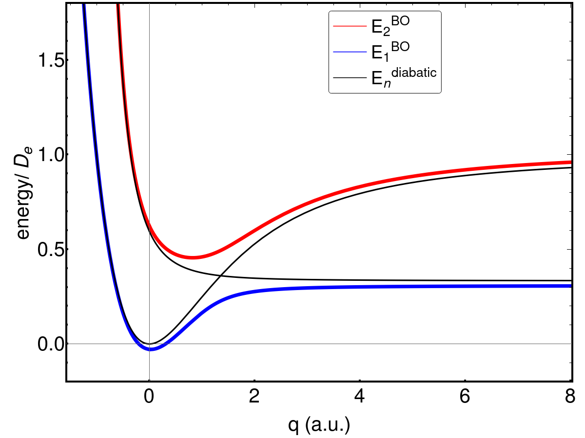
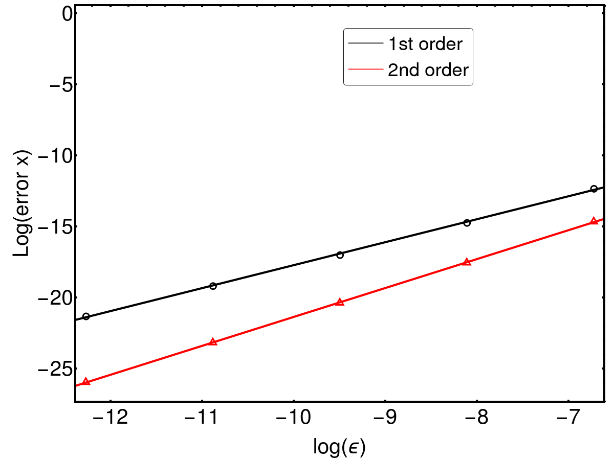
Figure 1: (a) Adiabatic and diabatic potential energy surfaces versus $q$; (b-d) Plots of the logarithmic error for first-order (black) and second-order (red) effective observables; (b) Best fit lines for the energy eigenvalues are $-3.37+1.51\log\epsilon$ and $-2.53+2.46\log\epsilon$; (c) Best fit lines for $\langle x\rangle$ are $-1.54+1.61\log\epsilon$ and $-1.00+2.03\log\epsilon$; (d) Best fit lines for $\langle x^{2}\rangle$ are $-1.83+1.49\log\epsilon$ and $-0.085+2.05\log\epsilon$.

The metric in this equation is trivial, $g_{0\mu\nu}=\delta_{\mu\nu}$, yet an important property of the first and second-order effective Schrödinger equations in Eqs. (9) and (3) is their coordinate invariance. To test the coordinate-invariant form of the equation in a nontrivial case, we change the independent variable according to

$$q=\sqrt{2}aL\sinh\frac{x}{L}{,}$$ (26)

which changes the kinetic energy operator to the standard form in Eq. (1) with $g_{0qq}=(2a^{2}+q^{2}/L^{2})^{-1}$ and the small parameter $\epsilon=2\hbar^{2}a^{2}/MD_{e}$. are used to express the Schrödinger equation as a generalized eigenvalue problem

$$\sum_{j}\mathcal{H}_{ij}\psi_{nj}=\lambda_{n}\sum_{j}S_{ij}\psi_{nj}{,}$$ (27)

where $\mathcal{H}_{ij}=\int\sqrt{g_{0qq}}\phi_{i}^{*}\mathcal{H}\phi_{j}dq$ and $S_{ij}=\int\sqrt{g_{0qq}}\phi_{i}^{*}\phi_{j}dq$.

Figure 1b shows that the error in the first-order ground state eigenvalue $\lambda_{0}^{(1)}$ is order $\epsilon^{3/2}$, while the error in the second-order eigenvalue $\lambda_{0}^{(2)}$ is order $\epsilon^{5/2}$. This is expected: the $p$th order effective Schrödinger equation provides an energy eigenvalue that is accurate to order $\epsilon^{p}$. Figures 1c shows that the error in $\langle x\rangle$ and $\langle x^{2}\rangle$ is order $\epsilon^{3/2}$ in the first-order approximation and order $\epsilon^{2}$ in the second-order approximation.

To further illustrate the first- and second-order effective Schrödinger equations, we now consider the linear $E\otimes e$ Jahn-Teller model, which is a two-dimensional model for which the Mead-Truhlar-Berry gauge potential is nontrivial. In a basis of odd $(|u\rangle)$ and even $(|g\rangle)$ electronic states, the Hamiltonian is

$$\mathcal{H} =-\frac{\hbar^{2}}{2M}\left(\frac{d^{2}}{dx_{1}^{2}}+\frac{d^{2}}{dx_{2}^{2}}\right)+\frac{K}{2}\big{(}x_{1}^{2}+x_{2}^{2}\big{)}I+g\left(\begin{array}[]{cc}x_{1}&-x_{2}\\ -x_{2}&-x_{1}\end{array}\right){.}$$ (30)

We can introduce polar coordinates $x=\sqrt{x_{1}^{2}+x_{2}^{2}}$ and $\phi=\arctan 2(x_{1},x_{2})$ and perform a separation of variables by transforming to a basis $|\pm\rangle=\frac{1}{\sqrt{2}}(|g\rangle\pm i|u\rangle)$ of current-carrying states and considering a state with angular momentum quantum number $j$:

$$|\psi_{nj}\rangle=\frac{1}{\sqrt{2\pi}}\left(\begin{array}[]{c}a_{nj}e^{i(j-1/2)\phi}\\ b_{nj}e^{i(j+1/2)\phi}\end{array}\right){.}$$ (33)

The quantum number $j$ takes half-integer values Moffitt and Liehr (1957); Moffitt and Thorson (1957); Longuet-Higgins et al. (1958) due to the nontrivial gauge potential.

To put the Schrödinger equation in the standard form of Eq. (1), we change the independent variable to $q=x/x_{0}$, where $x_{0}=g/K$ is the minimum of the radial potential $Kx^{2}/2-gx$, and define $\epsilon=\hbar^{2}K^{3}/Mg^{4}$. The Mead-Truhlar-Berry gauge potential in this model is $A_{\phi}=-j$ and the geometric potential is

$$V_{geo}=\frac{1}{8q^{2}}{.}$$ (34)

This fixes all of the potentials that appear in the first-order effective equation.

In polar coordinates, $g_{0qq}=1$, $g_{0\phi\phi}=q^{2}$, and the only nonzero element of the second-order Hermitian effective mass tensor is $h_{2\phi\phi}=1/4q$. The kinetic energy in Eq. (3) therefore contains the term

$$-\frac{1}{2}A_{\phi}g_{0}^{\phi\phi}h_{2\phi\phi}g_{0}^{\phi\phi}A_{\phi}=-\frac{j^{2}}{8q^{5}}{,}$$ (35)

which acts as a potential. Since $V_{2,geo}$ is zero, we have determined all of the potentials in the second-order effective equation, and our calculations verify that it reproduces the analytical results of O’Brien and Pooler O’Brien and Pooler (1979). For example, it reproduces the energy eigenvalue

$$\frac{\lambda_{n}^{(2)}}{\hbar\omega} =-\frac{1}{2}\epsilon^{-1/2}+n+\frac{1}{2}+\frac{j^{2}}{2}\epsilon^{1/2}+\frac{3j^{2}}{2}\epsilon(n+1/2)+\frac{j^{2}}{8}\epsilon^{3/2}[30(n^{2}+n+1/2)-1]-\frac{j^{4}}{2}\epsilon^{3/2}$$

$$\quad+\frac{5j^{2}}{16}\epsilon^{2}[28(n+1/2)^{3}+29(n+1/2)]-\frac{57j^{4}}{8}\epsilon^{2}(n+1/2){,}$$ (36)

which is accurate to order $\epsilon^{2}$ as expected. The eigenvalue of the first-order effective equation is accurate to order $\epsilon$. For $j=1/2$, the potential in Eq. (35) has been obtained Requist et al. (2017) from an asymptotic analysis of the nonlinear equations of the exact factorization method Gidopoulos and Gross (2014); Abedi et al. (2010); Hunter (1975). Unlike the theory developed here, the asymptotic analysis of O’Brien and Pooler and the analysis in Ref. Requist et al. (2017) are specifically tailored to a class of Jahn-Teller problems and not intended for light-heavy systems with many degrees of freedom.

III Conclusions

We have introduced a systematic adiabatic perturbation theory that yields a sequence of effective Schrödinger equations for the heavy component of a two-component system that are accurate to successively higher integer powers of $M^{-1}$. This can be viewed as a perturbation theory in the kinetic energy of the heavy component, which is quite different from other many-body perturbation theories. The fact that the gauge potential appears in the same way at every order may be important for perturbative descriptions of chiral vibrational modes in pseudorotating molecules and crystal defects Kendrick (1997); Perebeinos et al. (2005); Allen et al. (2005); Requist and Gross (2017); Ryabinkin et al. (2017); Kato et al. (2022); Lyakhov et al. (2023) and chiral phonons in solids Zhang and Niu (2014); Zhu et al. (2018); Ishito et al. (2023); Ueda et al. (2023).

References

- Born and Oppenheimer (1927) M. Born and R. Oppenheimer, Ann. Phys. 84, 457 (1927).
- Slater (1927) J. C. Slater, Proc. Nat. Acad. Sci. 13, 423 (1927).
- Littlejohn and Weigert (1993) R. G. Littlejohn and S. Weigert, Phys. Rev. A 48, 924 (1993).
- Weigert and Littlejohn (1993) S. Weigert and R. G. Littlejohn, Phys. Rev. A 47, 3506 (1993).
- Mead and Truhlar (1979) C. A. Mead and D. G. Truhlar, J. Chem. Phys. 70, 2284 (1979).
- Ferrari (2007) A. C. Ferrari, Solid State Commun. 143, 47 (2007).
- Basko et al. (2009) D. M. Basko, S. Piscanec, and A. C. Ferrari, Phys. Rev. B 80, 165413 (2009).
- Dean et al. (2010) M. P. M. Dean, C. A. Howard, S. S. Saxena, and M. Ellerby, Phys. Rev. B 81, 045405 (2010).
- De Fillipis et al. (2010) G. De Fillipis, V. Cataudella, R. Citro, C. A. Perroni, A. S. Mishchenko, and N. Nagaosa, Eur. Phys. Lett. 91, 47007 (2010).
- Klimin et al. (2016) S. N. Klimin, J. Tempere, and J. T. Devreese, Phys. Rev. B 94, 125206 (2016).
- Ponosov and Streltsov (2016) Y. S. Ponosov and S. V. Streltsov, Phys. Rev. B 94, 214302 (2016).
- Ponosov and Streltsov (2017) Y. S. Ponosov and S. V. Streltsov, Phys. Rev. B 96, 214503 (2017).
- Lazzeri and Mauri (2006) M. Lazzeri and F. Mauri, Phys. Rev. Lett. 97, 266407 (2006).
- Bock et al. (2006) N. Bock, D. C. Wallace, and D. Coffey, Phys. Rev. B 73, 075114 (2006).
- Pisana et al. (2007) S. Pisana, M. Lazzeri, C. Casiraghi, K. S. Novoselov, A. K. Geim, A. C. Ferrari, and F. Mauri, Nature Mat. 6, 198 (2007).
- Piscanec et al. (2007) S. Piscanec, M. Lazzeri, J. Robertson, A. C. Ferrari, and F. Mauri, Phys. Rev. B 75, 035427 (2007).
- Calandra et al. (2007) M. Calandra, M. Lazzeri, and F. Mauri, Physica C 456, 38 (2007).
- Caudal et al. (2007) N. Caudal, A. M. Saitta, M. Lazzeri, and F. Mauri, Phys. Rev. B 75, 115423 (2007).
- Saitta et al. (2008) A. M. Saitta, M. Lazzeri, M. Calandra, and F. Mauri, Phys. Rev. Lett. 100, 226401 (2008).
- Calandra et al. (2010) M. Calandra, G. Profeta, and F. Mauri, Phys. Rev. B 82, 165111 (2010).
- Gonze et al. (2011) X. Gonze, P. Boulanger, and M. Côté, Ann. Phys. (Berlin) 523, 168 (2011).
- Cannuccia and Marini (2012) E. Cannuccia and A. Marini, Eur. Phys. J. B 85, 320 (2012).
- Marini et al. (2015) A. Marini, S. Poncé, and X. Gonze, Phys. Rev. B 91, 224310 (2015).
- Poncé et al. (2015) S. Poncé, Y. Gillet, J. Laflamme Janssen, A. Marini, M. Verstraete, and X. Gonze, J. Chem. Phys. 143, 102813 (2015).
- Antonius et al. (2015) G. Antonius, S. Poncé, E. Lantagne-Hurtubise, G. Auclair, X. Gonze, and M. Côté, Phys. Rev. B 92, 085137 (2015).
- M. d’Astuto et al. (2016) M. d’Astuto et al., Phys. Rev. B 93, 180508(R) (2016).
- Gali et al. (2016) A. Gali, T. Demján, M. Vörös, G. Thiering, E. Cannuccia, and A. Marini, Nature Commun. 7, 11327 (2016).
- Nery and Allen (2016) J. P. Nery and P. B. Allen, Phys. Rev. B 94, 115135 (2016).
- Allen and Nery (2017) P. B. Allen and J. P. Nery, Phys. Rev. B 95, 035211 (2017).
- Giustino (2017) F. Giustino, Rev. Mod. Phys. 89, 015003 (2017).
- Long and Prezhdo (2017) R. Long and O. V. Prezhdo, J. Phys. Chem. Lett. 8, 193 (2017).
- Zhou et al. (2017) X. Zhou, L. Li, H. Dong, A. Giri, P. E. Hopkins, and O. V. Prezhdo, J. Phys. Chem. C 121, 17488 (2017).
- Caruso et al. (2017) F. Caruso, M. Hoesch, P. Achatz, J. Serrano, M. Krisch, E. Bustarret, and F. Giustino, Phys. Rev. Lett. 119, 017001 (2017).
- Nery et al. (2018) J. P. Nery, P. B. Allen, G. Antonius, L. Reining, A. Miglio, and X. Gonze, Phys. Rev. B 97, 115145 (2018).
- Marini and Pavlyukh (2018) A. Marini and Y. Pavlyukh, Phys. Rev. B 98, 075105 (2018).
- Novko (2018) D. Novko, Phys. Rev. B 98, 041112(R) (2018).
- Requist et al. (2019) R. Requist, C. R. Proetto, and E. K. U. Gross, Phys. Rev. B 99, 165136 (2019).
- Pellegrini et al. (2022) C. Pellegrini, A. Sanna, R. Requist, and E. K. U. Gross, J. Phys.: Condens. Matter 34, 183002 (2022).
- Talantsev (2023) E. F. Talantsev, Symmetry 15, 1632 (2023).
- Girotto and Novko (2023) N. Girotto and D. Novko, Phys. Rev. B 107, 064310 (2023).
- Brousseau-Couture et al. (2023) V. Brousseau-Couture, X. Gonze, and M. Côté, Phys. Rev. B 107, 115173 (2023).
- Makhov et al. (2014) D. V. Makhov, W. J. Glover, T. J. Martinez, and D. V. Shalashilin, J. Chem. Phys. 141, 054110 (2014).
- Min et al. (2015) S. K. Min, F. Agostini, and E. K. U. Gross, Phys. Rev. Lett. 115, 073001 (2015).
- Requist et al. (2016) R. Requist, F. Tandetzky, and E. K. U. Gross, Phys. Rev. A 93, 042108 (2016).
- Requist and Gross (2016) R. Requist and E. K. U. Gross, Phys. Rev. Lett. 117, 193001 (2016).
- Li et al. (2018) C. Li, R. Requist, and E. K. U. Gross, J. Chem. Phys. 148, 084110 (2018).
- Crespo-Otero and Barbatti (2018) R. Crespo-Otero and M. Barbatti, Chem. Rev. 118, 7026 (2018).
- Loncarić et al. (2019) I. Loncarić, M. Alducin, J. I. Juaristi, and D. Novko, J. Phys. Chem. Lett. 10, 1043 (2019).
- Agostini and Curchod (2019) F. Agostini and B. F. E. Curchod, Computational Molecular Science 9, 1 (2019).
- Martinazzo and Burghardt (2022) R. Martinazzo and I. Burghardt, Phys. Rev. Lett. 128, 206002 (2022).
- Villaseco Arribas et al. (2022) E. Villaseco Arribas, F. Agostini, and N. T. Maitra, Molecules 27, 4002 (2022).
- Kocák et al. (2023) J. Kocák, E. Kraisler, and A. Schild, Phys. Rev. Research 5, 013016 (2023).
- Manfredi et al. (2023) G. Manfredi, A. Rittaud, and C. Tronci, J. Phys. A: Math. Theor. 56, 154002 (2023).
- Gardner et al. (2023) J. Gardner, S. Habershon, and R. J. Maurer, J. Phys. Chem. C 127, 15257 (2023).
- Bombín et al. (2023) R. Bombín, A. S. Muzas, D. Novko, J. Iñaki Juaristi, and M. Alducin, Phys. Rev. B 108, 045409 (2023).
- Athavale et al. (2021) V. Athavale, X. Bian, Z. Tao, Y. Wu, T. Qiu, J. Rawlinson, R. Littlejohn, and J. E. Subotnik, arxiv:2308.14621 (2021).
- Mead (1980) C. A. Mead, J. Chem. Phys. 72, 3839 (1980).
- Berry (1984) M. V. Berry, Proc. Roy. Soc. Lond. A 392, 45 (1984).
- Provost and Vallee (1980) J. P. Provost and G. Vallee, Commun. Math. Phys. 76, 289 (1980).
- Berry (1989) M. V. Berry, “The quantum phase, five years after,” (1989) pp. 7–28, in ref. Shapere and Wilczek (1989).
- Berry and Lim (1990) M. V. Berry and R. Lim, J. Phys. A: Math. Gen 23, L655 (1990).
- Teufel (2003) S. Teufel, Adiabatic perturbation theory in quantum dynamics (Springer, Berlin, 2003).
- Requist (2023) R. Requist, accepted by J. Phys. A: Math. Theor.; arxiv:2206.01716 (2023).
- Littlejohn and Reinsch (1997) R. G. Littlejohn and M. Reinsch, Rev. Mod. Phys. 69, 213 (1997).
- Moffitt and Liehr (1957) W. Moffitt and A. D. Liehr, Phys. Rev. 106, 1195 (1957).
- Moffitt and Thorson (1957) W. Moffitt and W. Thorson, Phys. Rev. 108, 1251 (1957).
- Longuet-Higgins et al. (1958) H. C. Longuet-Higgins, U. Öpik, M. H. L. Pryce, and R. A. Sack, Proc. R. Soc. London, Ser. A 244, 1 (1958).
- O’Brien and Pooler (1979) M. C. M. O’Brien and D. R. Pooler, J. Phys. C: Solid State Phys. 12, 311 (1979).
- Requist et al. (2017) R. Requist, C. R. Proetto, and E. K. U. Gross, Phys. Rev. A 96, 062503 (2017).
- Gidopoulos and Gross (2014) N. I. Gidopoulos and E. K. U. Gross, Phil. Trans. Roy. Soc. A 372, 20130059 (2014).
- Abedi et al. (2010) A. Abedi, N. T. Maitra, and E. K. U. Gross, Phys. Rev. Lett. 105, 123002 (2010).
- Hunter (1975) G. Hunter, Int. J. Quantum Chem. 9, 237 (1975).
- Kendrick (1997) B. Kendrick, Phys. Rev. Lett. 79, 2431 (1997).
- Perebeinos et al. (2005) V. Perebeinos, P. B. Allen, and M. Pederson, Phys. Rev. A 72, 012501 (2005).
- Allen et al. (2005) P. B. Allen, A. G. Abanov, and R. Requist, Phys. Rev. A 71, 043203 (2005).
- Requist and Gross (2017) R. Requist and E. K. U. Gross, Jahrbuch der Max-Planck-Gesellschaft (2016/2017), 10.17617/1.59.
- Ryabinkin et al. (2017) I. G. Ryabinkin, L. Joubert-Doriol, and A. F. Izmaylov, Acc. Chem. Res. 50, 1785 (2017).
- Kato et al. (2022) A. Kato, H. M. Yamamoto, and J. Kishine, Phys. Rev. B 105, 195117 (2022).
- Lyakhov et al. (2023) A. D. Lyakhov, A. S. Ovchinnikov, I. G. Bostrem, and J. Kishine, Phys. Rev. B 108, 115429 (2023).
- Zhang and Niu (2014) L. Zhang and Q. Niu, Phys. Rev. Lett. 112, 085503 (2014).
- Zhu et al. (2018) H. Zhu, J. Yi, M.-Y. Li, J. Xiao, L. Zhang, C.-W. Yang, R. A. Kaindl, L.-J. Li, Y. Wang, and X. Zhang, Science 359, 579 (2018).
- Ishito et al. (2023) K. Ishito, H. Mao, K. Kobayashi, Y. Kousaka, Y. Togawa, H. Kusunose, J. Kishine, and T. Satoh, Chirality 35, 338 (2023).
- Ueda et al. (2023) H. Ueda, M. García-Fernández, S. Agrestini, C. P. Romao, J. van den Brink, N. A. Spaldin, K.-J. Zhou, and U. Staub, Nature 618, 946 (2023).
- Shapere and Wilczek (1989) A. Shapere and F. Wilczek, eds., Geometric phases in physics (World Scientific, Singapore, 1989).