Histogram-less LiDAR through SPAD response linearization

capbtabboxtable[][]

We present a new method to acquire the 3D information from a SPAD-based direct-Time-of-Flight (d-ToF) imaging system which does not require the construction of a histogram of timestamps and can withstand high flux operation regime. The proposed acquisition scheme emulates the behavior of a SPAD detector with no distortion due to dead time, and extracts the ToF information by a simple average operation on the photon timestamps ensuring ease of integration in a dedicated sensor and scalability to large arrays. The method is validated through a comprehensive mathematical analysis, whose predictions are in agreement with a numerical Monte Carlo model of the problem. Finally, we show the validity of the predictions in a real d-ToF measurement setup under challenging background conditions well beyond the typical pile-up limit of 5% detection rate up to a distance of 3.8 m.

1 Introduction and related work

Spatial perception enabled by 3D imaging techniques is constantly gaining interest for industrial [1], automotive [2], space [3] and consumer applications. As an example, the required level of self-awareness of autonomous driving vehicles demands for 3D imaging systems with high resolution and high frame rate. Unfortunately, these requirements are in conflict, constraining engineers to performance-limiting tradeoffs. In this paper we focus on Light Detection And Ranging (LiDAR) / direct-Time-of-Flight (d-ToF) measurement based on Single-Photon Avalanche Diodes (SPAD), which is one of the most promising among active techniques [4]. In a SPAD-based d-ToF measurement, the distance is extracted by measuring the traveling time of a pulse of light projected from the source and reflected back by the target to a detector that consists of a SPAD operating as a photon-to-edge converter, coupled to a photon timestamping circuit (usually a Time-to-Digital Converter (TDC) or a Time-to-Amplitude Converter (TAC)) [5, 6, 7]. Due to hardware limitations, such as the detector dead-time and the statistical nature of photons, together with the presence of uncorrelated background light, a number of observations are usually accumulated into a histogram memory to enhance the signal to noise ratio and extract the target distance by means of signal processing techniques [8, 9].

The increased interest in Advanced Driver Assistance Systems (ADAS), where 3D vision is a pillar, is focusing the attention of researchers in developing techniques to increase the robustness of such systems against the effect of background light and against possible interference from similar devices. Concerning the problem of background light, one of the most effective and widespread technique is known as photon coincidence, which exploits the temporal proximity of photons belonging to the reflected laser pulse to filter out unwanted background photons which are more likely to be temporally sparse [10, 11]. With a different method, based on a smart accumulation technique by Yoshioka et al. [12], the signal to noise ratio (SNR) is increased by merging the information from pixels observing similar regions of the scene. A different approach has been recently proposed by Manuzzato et al. [13], where a per-pixel circuit is able to automatically decrease the SPAD sensitivity reducing the probability of saturation in case of high background intensities, favoring the detection of laser photons. Yet another technique is known as time-gating, where by means of a search procedure several sub-ranges of the scene are measured, increasing the SNR at the expense of an increased acquisition time [14]. Regarding the problem of mutual interference, Ximenes et al. [15] propose a spread-spectrum based technique, where the laser emission time is randomized from device to device, spreading any other interference below the level of the signal of interest. Another solution is based on the emission of two laser pulses whose temporal relationship is different from device to device and used to actively discard unwanted interference [16, 17].

These techniques, however, cannot cope with very high fluxes because of two fundamental problems. First, the histogram of timestamps appears distorted due to the dead-time of SPAD detectors and timestamping circuits, which translates into a non-linear response of the system to the incident flux of photons over time. It is a widely held belief that the upper photon flux limit that still results in a negligibly distorted histogram is given by 5% of detected photons per laser cycle [18]. Second, the amount of data generated by the sensor is too large to scale to a large number of pixels. Rapp et al. [19] overcome the former problem by linearizing the histogram through a Markov chain model of the photon detection times. By using this method, the system can cope with up to 5 photoelectrons per illumination cycle. Gyongy et al. [20] mitigate the second problem by upscaling a low resolution depth image based on a high resolution intensity image. A similar approach is used by Ruget et al. [21], where the native resolution of a depth image from a SPAD camera is increased by means of a deep neural network. Still the bottleneck is represented by the necessity to build and transfer a histogram of timestamps for each pixel in the image from which the ToF is extracted.

One strategy to reduce the bandwidth requirement on the amount of data which is transferred from the chip to the controller (usually an FPGA or $\mu$C) is to integrate the histogram, or part of it, directly on chip. Several solutions are proposed in the literature to integrate histogramming capability on-chip [22, 23, 24, 25, 26, 27, 28, 29, 30, 31], but despite the advantage in bandwidth performance compared to other solutions where the histogram is built off-chip [10, 11, 15, 14, 13], still many limitations are present. In general, the on-chip realization of either a partial or full histogram requires additional area, which can be obtained by either reducing the fill factor or by using expensive 3D-stacked solutions.

With the so-called partial approach [24, 26, 16, 27, 29, 31, 30], a reduced histogram memory is available on-chip, therefore requiring a search procedure to identify the location of the ensemble of histogram bins containing the laser peak. In the literature, two techniques have been described to implement a partial histogram behavior. With the so-called zooming technique [24, 26, 16, 30], at the beginning of the measurement the reduced set of histogram bins is spread across the entire distance range. By counting the number of photons detected on each bin, the reduced set of histogram bins is concentrated over several iterations on a shorter range, thus achieving the desired resolution on the estimated target distance. With the other technique, called sliding, the subset of histogram bins is already set to the desired resolution, thus covering only a small portion of the range. Again by means of several iterations, the subset of histogram bins slides across the entire range, and the number of photons at each iteration is used to estimate the target distance. Despite the intrinsic differences between the two methods, for both of them, as outlined by Taneski et al. [32], a laser power penalty occurs as more laser shots are required to find the laser peak location.

A full histogram approach is possible with resource sharing, e.g., by reallocating the same histogram circuitry to several pixels, as described by Kumagai et al. [28]. However, resource sharing resulted in only $\approx 27\%$ of the chip area dedicated to the SPAD array, requiring a very high clock frequency of 500 MHz and the design of a 3D stacked solution with a complex scanning illumination approach.

In this paper we propose for the first time a robust method supported by a rigorous mathematical model to extract the 3D information from a set of acquired timestamps without the need to build a histogram, which can also sustain high photon fluxes, enabling the possibility to operate beyond the standard limit of 5% detection rate [18] for pile-up distortion. The method can be implemented using only two registers and one accumulator for each pixel. With such a low amount of resources, the per-pixel memory requirement is reduced by more than 3 orders of magnitude compared to standard d-ToF architectures (off-chip histogram) [15, 14], and by a factor of $\simeq 5$ compared to architectures with on-chip, full histogramming capability [33]. We reach the goal in two steps. First, we propose and evaluate an algorithm to efficiently extract the target distance from a set of timestamps based on a simple on-the-fly average operation, which does not require the allocation of a histogram memory. Then, since the proposed algorithm works on the assumption that the detector response is linear, we present two acquisition schemes that can be easily implemented on chip and emulate the behavior of a single photon detector with no dead-time, providing the desired linear response to the input flux of photons. The proposed method is supported by analytical and numerical (Monte Carlo) models and has been validated experimentally up to a distance of 3.8 meters (mainly limited by the sensor used for characterization [34]) under a background light equivalent to 85 kilolux and beyond the standard 5% rule for pile-up distortion [18].

The paper is organized as follows. In Section 2, a typical d-ToF acquisition system with the most important parameters of concern is described and preliminary considerations on a histogram-less acquisition approach are provided with a first validation by means of a Monte Carlo model. In Section 3, we provide the analytical proof of the proposed acquisition method, while in Section 4 we explain in detail two acquisition schemes which are needed to emulate the response of a linear detector, together with a comparison against state-of-the art sensors in terms of memory requirement, scalability and tolerance to high background flux. In Section 5, we provide measurement results from an existing SPAD-based d-ToF sensor, showing that the proposed acquisition and extraction schemes are capable of successfully computing the ToF without the need for a histogram of timestamps. Finally, we discuss future perspectives to advance the results found in this work in Section 6.

2 Preliminary validation

In this section, we present the principle of operation of a SPAD-based d-ToF system with preliminary considerations and Monte Carlo simulations on the histogram-less approach which will be further developed in the paper.

2.1 Typical d-ToF operation

A typical d-ToF image acquisition requires a pulsed laser and a time-resolved, single photon image sensor with photon timestamping capabilities. It works by sending periodic laser pulses and then measuring the arrival time, or timestamp, of the first detected photons reflected by the target following each pulse. Due to space and bandwidth limitations, the number of photon timestamps generated per laser pulse is typically limited to one.

In principle, a single laser pulse, and thus a single timestamp, would be sufficient to estimate the time of flight. However, due to the presence of uncorrelated background events (from both external light sources or internal SPAD Dark Count Rate (DCR)) and of shot noise, the first detected photon may not be from the laser pulse, so that several repetitions are needed to discriminate the different contributions. To do so, the timestamps measured during the acquisition process are collected in a histogram memory that records how many times each timestamp has been observed. This provides a convenient representation of the temporal distribution of the arrival times, as shown in the example of Figure 1. In a system capable of acquiring only one photon (the first), the distribution of the arrival times is a piece-wise exponential curve, where each segment is described by:

$$P_{i}(t)=A_{i}\cdot e^{-\lambda_{i}\cdot t}$$ (1)

whose intensity (rate) $\lambda_{i}$ depends on the intensity of background light, dark counts and laser echo. Table 1 summarizes the most important parameters of the detection process.

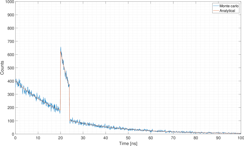
Figure 1: Simulated distribution of timestamps in a typical d-ToF system able to record 1 photon per acquisition, with a ToF of 20 ns and a laser pulse duration $T_{W}$ of 4 ns. The histogram is composed of $10^{5}$ timestamps, with a bin size of 100 ps. Superimposed to the Monte Carlo simulation, we show also the analytical exponential distribution.

Table 1: List of parameters for a typical d-ToF acquisition.

Parameter	Unit	Description
$\lambda_{B}$	$s^{-1}$	Background events rate
$\lambda_{S}$	$s^{-1}$	Reflected laser events rate
$T_{W}$	$s$	Laser pulse duration
ToF	$s$	Time of flight

The ToF is typically estimated from the histogram by finding the location of its peak or of a sharp rising edge, which likely belongs to the reflected laser pulse. The histogram of timestamps contains all the relevant information to properly estimate the time of flight, and represents the gold standard processing technique in the field of SPAD-based d-ToF systems. Unfortunately, the histogram requires a considerable amount of resources in terms of memory, bandwidth and power, as it requires the readout of every timestamp from the sensor for processing by an external controller (FPGA or $\mu$C). Even with the latest implementations where the histogram is available on-chip, the required amount of resources is considerable. As an example, a 10-m-range $128\times 128$ LiDAR system with a 100 ps time resolution and 8 bit histogram depth requires approximately 10 MB of memory.

2.2 Histogram-less approach

Intuitively, if no background events are present, and neglecting the width of the laser pulse, we could estimate the time-of-flight without the need to build a histogram. This can be achieved by simply calculating the average of the continuous stream of laser-only timestamps. To extend the above method to scenarios where background events are also present, we need to eliminate their contribution to the average. Again, intuitively, this can be accomplished by dividing the measurement into two acquisitions. The first is performed with the laser turned off, and is used to estimate the contribution of the background light only, by computing the average $\bar{t}_{bg}$ of the recorded timestamps. The same operation is repeated in the second acquisition with the joint contribution of background and laser timestamps, resulting in a total average time $\bar{t}_{tot}$. In principle, the time of flight should be proportional to the difference between the two averages, with the contribution of the background canceling out:

$$\emph{ToF}\propto\bar{t}_{tot}-\bar{t}_{bg}.$$ (2)

This approach, however, relies on the superposition property which does not hold, as SPADs are non-linear detectors.

More specifically, the problem lies in the dead time of the detection process, which depends upon the SPAD dead-time itself, on the limited bandwidth of the timestamping circuit and also on the limited memory available, blinding the measurement channel for some time after each detection. With this limitation, the detection of a photon belonging to the laser echo does prevent a later photon from being potentially detected, resulting in a distortion of the statistics. In particular, the amount of background photons which contribute to $\bar{t}_{tot}$ in the second acquisition (with the laser turned on) is underestimated. This behavior can be observed on the histograms of Figure 2, where the distribution of timestamps in different scenarios are compared, emphasizing the estimation error. Furthermore, the greater the laser echo intensity, the higher the number of background photons that are underestimated.

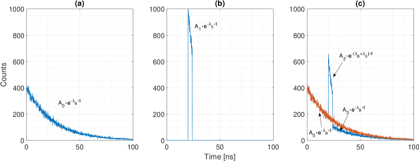
Figure 2: Simulated distribution of timestamps in a typical d-ToF acquisition. In (a) and (b), the distributions of background-only events (with rate $\lambda_{B}$) and laser-only events (with rate $\lambda_{S}$), respectively, are shown. In (c), the distribution of the combination of background and laser events is reported, graphically showing that the superposition property does not hold due to the non-linear behavior of the detection process. In particular, the portion of background events after the laser peak are underestimated, as only one photon per acquisition can be detected. For each contribution, the amplitude terms of the exponential ($A_{0}$, $A_{1}$, $A_{2}$ and $A_{3}$) are reported, with $A_{3}<A_{0}$ due to the SPAD non-linearity.

This can also be seen analytically by computing explicitly the cumulative distribution function $F$ of the random variable $T$ associated to the first photon detection time, defined as $F(t):=\mathbb{P}(T\in[0,t])$. If $t\in[0,\emph{ToF}]$ then the incoming photon necessarily belongs to the background, hence

$$F(t)=\mathbb{P}\left(T\in[0,t]\right)=1-e^{-\lambda_{B}t}\,$$

If $t\in(\emph{ToF},\emph{ToF}+T_{W}]$, then

$$F(t) =\mathbb{P}(T\in[0,\emph{ToF}])+\mathbb{P}(T\in(\emph{ToF},t])$$

$$=1-e^{-\lambda_{B}\emph{ToF}}+e^{-\lambda_{B}\emph{ToF}}\left(1-e^{-(\lambda_{S}+\lambda_{B})(t-\emph{ToF})}\right)\,$$

Finally, for $t>\emph{ToF}+T_{W}$ we have:

$$F(t) =\mathbb{P}(T\in[0,\emph{ToF}])+\mathbb{P}(T\in(\emph{ToF},\emph{ToF}+T_{W}])+\mathbb{P}(T\in(\emph{ToF}+T_{W},t])$$

$$=1-e^{-\lambda_{B}\emph{ToF}}+e^{-\lambda_{B}\emph{ToF}}\left(1-e^{-(\lambda_{S}+\lambda_{B})T_{W}}\right)+e^{-\lambda_{B}\emph{ToF}}e^{-(\lambda_{S}+\lambda_{B})T_{W}}\left(1-e^{-\lambda_{B}(t-\emph{ToF}-T_{W})}\right)\,$$

The probability density $f$ of the distribution of $T$, where $F(t)=\int_{-\infty}^{t}f(u)du$, can be easily computed by means of the formula $f(t)=F^{\prime}(t)$, yielding:

$$f(t)=\begin{cases}\lambda_{B}e^{-\lambda_{B}t}&t\in[0,\emph{ToF}]\\ (\lambda_{S}+\lambda_{B})e^{\lambda_{S}\emph{ToF}}e^{-(\lambda_{S}+\lambda_{B})t}&t\in(\emph{ToF},\emph{ToF}+T_{W}]\\ \lambda_{B}e^{-\lambda_{S}T_{W}}e^{-\lambda_{B}t}&t>\emph{ToF}+T_{W}\end{cases}$$

while the average first arrival time is given by

$${\mathbb{E}}[T]=\int_{0}^{+\infty}tf(t)dt=\frac{1-e^{-\lambda_{B}\emph{ToF}}}{\lambda_{B}}+\frac{e^{-\lambda_{B}\emph{ToF}}(1-e^{-(\lambda_{S}+\lambda_{B})T_{w}})}{\lambda_{S}+\lambda_{B}}+\frac{e^{-\lambda_{S}T_{W}}e^{-\lambda_{B}(\emph{ToF}+T_{W})}}{\lambda_{B}}$$ (3)

As shown in Equation (3), the average detection time depends non-linearly on two parameters ($\lambda_{S}$ and ToF). This confirms that it is not possible to uniquely extract the ToF from the aforementioned acquisition method, since the average of the timestamps acquired in the second acquisition, $\bar{t}_{tot}$, which is governed by the probability of detection of laser photons, also depends on the $\lambda_{S}$ parameter, which depends not only on the ToF, but also on the target reflectivity. One could try to compensate for the error, however this requires measuring also the intensity of the received laser light (which affects the error), introducing an extra variable which is hard to estimate, invalidating the procedure.

Conversely, a linear detector, with no dead-time, is able to timestamp every photon which falls within the acquisition window. In this case, the histograms shown in Figure 2 become linear in time, as shown in Figure 3.

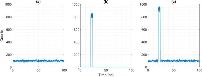
Figure 3: Distribution of timestamps obtained with a linear detection process, i.e., with no dead-time limitation. The distributions are uniform, since we are now considering the absolute arrival time of detected photons with respect to the beginning of the acquisition window. With this approach, it is possible to safely subtract the background contribution in (a) from the combined measurement in (c). As the superposition property holds in this case, there is no longer an under-weighting condition of background counts after the laser pulse peak in the histogram (c).

One can then extract the ToF with the proposed two-step procedure. In the first step, we measure the total number of background events, $N_{bg}$, and their average absolute arrival time, $\bar{t}_{bg}$. In the second step, with the combination of both background and laser events, we measure the total number of events and their average absolute arrival time, denoted $N_{tot}$ and $\bar{t}_{tot}$. Because the superposition property holds, the difference $N_{tot}-N_{bg}$ is equal to the amount of photons from the reflected laser source. We can then extract the ToF by properly weighting each average timestamp measurement with the relative photon count contribution:

$$N_{tot}\cdot\overline{t}_{tot}=N_{bg}\cdot\overline{t}_{bg}+(\emph{ToF}+\overline{t}_{l})\cdot(N_{tot}-N_{bg})\,$$ (4)

where $\overline{t}_{l}$ is the average arrival time of the laser photons referred to the laser emission time in the absence of background light (i.e., $\lambda_{B}=0$ and $\emph{ToF}=0$). The value $\overline{t}_{l}$ is a characteristic parameter of the laser source, which can be experimentally estimated by means of an initial calibration. The proposed extraction method does not require the allocation of histogram memory, and needs only two counters to store $N_{bg}$ and $N_{tot}$, and two accumulators to compute $\bar{t}_{bg}$ and $\bar{t}_{tot}$ reducing the memory requirements by more than three orders of magnitude compared to recent long-range high-resolution d-ToF sensors [15, 14]. We can further reduce the amount of resources down to a single accumulator, needed to store $\bar{t}_{tot}$, and two counters for $N_{bg}$ and $N_{tot}$, because a constant background throughout the acquisition window leads to an average background time $\bar{t}_{bg}$ of $T_{acq}/2$. In this case, Equation (4) turns into the simpler form:

$$N_{tot}\cdot\overline{t}_{tot}=N_{bg}\cdot\frac{T_{acq}}{2}+(ToF+\overline{t}_{l})\cdot(N_{tot}-N_{bg})\,$$ (5)

which yields:

$$\emph{ToF}=\frac{N_{tot}\bar{t}_{tot}-N_{bg}\frac{T_{acq}}{2}}{N_{tot}-N_{bg}}-\overline{t}_{l}$$ (6)

We have simulated this extraction method with a Monte Carlo simulator [35] by sweeping the parameters $\lambda_{S}$ and $\lambda_{B}$ in the range $[10^{6}-10^{8}]$ and $[10^{5}-10^{9}]$, respectively. For each pair of $\lambda_{S}$ and $\lambda_{B}$ values, $10^{4}$ measurements have been acquired with the ToF value set to 25 ns. The resulting ToF, obtained from Equation (4), is shown in Figure 4 with the correct estimation over a wide range of $\lambda_{B},\lambda_{S}$ pairs, failing only when the $\lambda_{S}/\lambda_{B}$ ratio is too low even for a classic histogram-based approach.

In the next section, we provide a rigorous mathematical analysis which proves the results briefly introduced with Equation (6) from the underlying statistical distribution of photons.

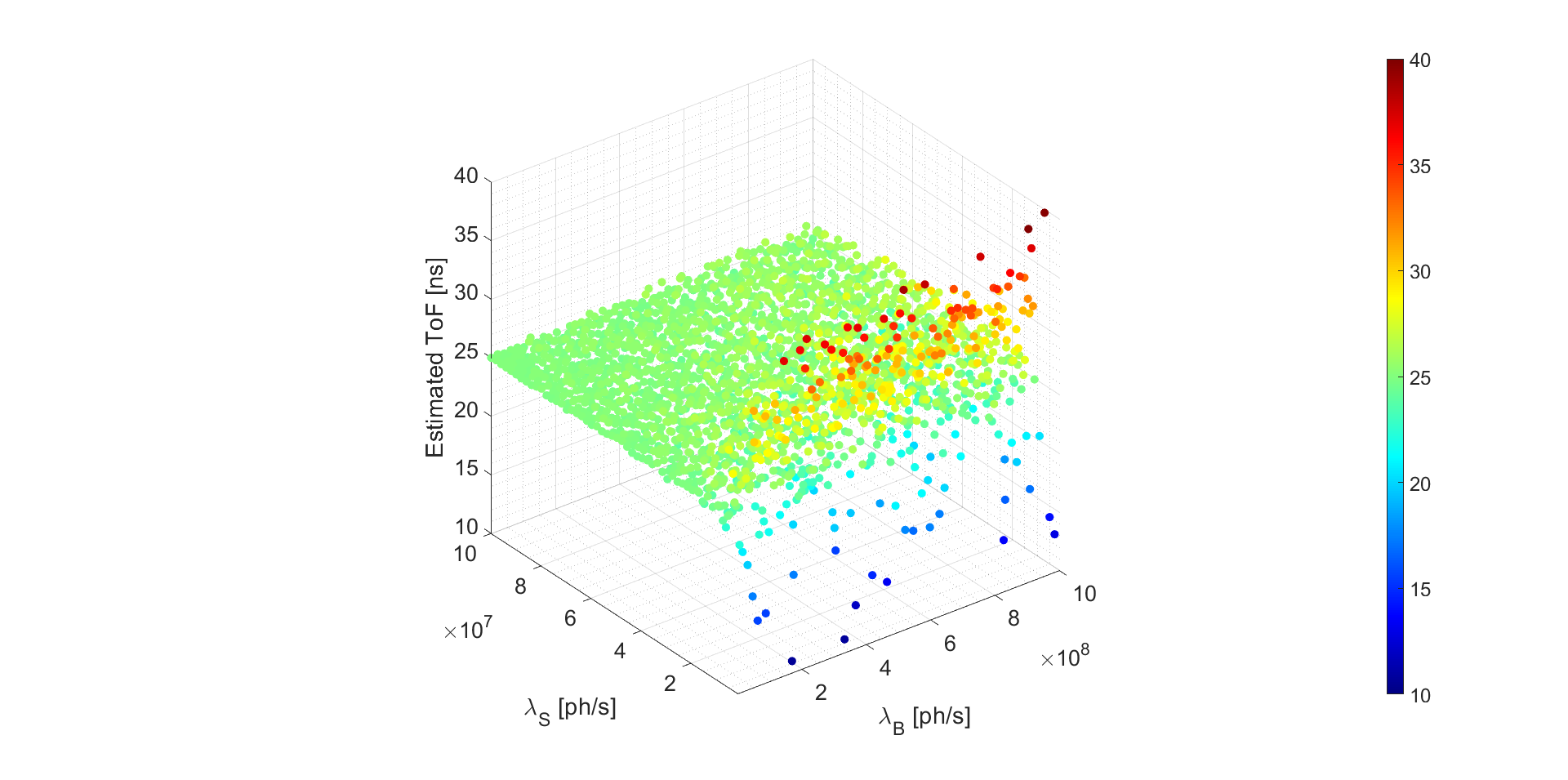
Figure 4: Preliminary Monte Carlo simulation results showing the ToF computed with the proposed acquisition method with the hypothesis of an ideal linear detector. The ToF can be properly estimated over a wide range of $\lambda_{B},\lambda_{S}$ pairs.

3 Mathematical analysis

This section proves the validity of the method described above analytically. In the following, we shall denote the duration of the acquisition window by $T_{acq}$, assume the laser echo to entirely occur within it, i.e., $T_{acq}\gg\emph{ToF}+T_{W}$, and denote the time-dependent intensity of the laser pulse by the function $\lambda_{S}:[0,T_{W}]\to{\mathbb{R}}$. The flux of photons can be modeled by a counting process $(N_{t})_{t\in[0,T_{acq}]}$ obtained as the sum of two independent Poisson processes: $(N^{B}_{t})_{t\in[0,T_{acq}]}$, with intensity $\lambda_{B}$, describing the background flux of photons, and $(N^{S}_{t})_{t\in[\emph{ToF},\emph{ToF}+T_{W}]}$, describing the signal. In particular, the process $(N^{S}_{t})_{t\in[\emph{ToF},\emph{ToF}+T_{W}]}$ is modeled through an inhomogeneous Poisson process with time dependent intensity $(\tilde{\lambda}_{S}(t))_{t\in[\emph{ToF},\emph{ToF}+T_{W}]}$ given by $\tilde{\lambda}_{S}(t):=\lambda_{S}(t-\emph{ToF})$. Hence, the overall flux of photons reaching the SPAD is given by an inhomogeneous Poisson process $(N_{t}))_{t\in[0,T_{acq}]}$ with varying intensity $\lambda$ given by

$$\lambda(t)=\begin{cases}\lambda_{B}&t\in[0,\emph{ToF})\cup[\emph{ToF}+T_{W},T_{acq}]\\ \lambda_{B}+\tilde{\lambda}_{S}(t)&t\in[\emph{ToF},\emph{ToF}+T_{W})\end{cases}$$

Hence, we can prove that, given $n$ photons detected in the interval $I=[0,T_{acq}]$, the $n$ detection times are independent and distributed on $[0,T_{acq}]$ with a distribution density function $f:[0,T_{acq}]\to{\mathbb{R}}$ given by

$$f(t)=\begin{cases}\frac{\displaystyle\lambda_{B}}{\displaystyle\lambda_{B}T_{acq}+\int_{0}^{T_{W}}\lambda_{S}(u)du}&t\in[0,\emph{ToF})\cup[\emph{ToF}+T_{W},T_{acq}]\\ &\\ \frac{\displaystyle\lambda_{B}+\lambda_{S}(t-\emph{ToF})}{\displaystyle\lambda_{B}T_{acq}+\int_{0}^{T_{W}}\lambda_{S}(u)du}&t\in[\emph{ToF},\emph{ToF}+T_{W})\end{cases}$$ (7)

Indeed, by considering a partition $\{I_{j}\}_{j=1,\dots,m}$ of the interval $I=[0,T_{acq}]$, the independence of the increments of the inhomogeneous Poisson processes $(N_{t})_{t\in[0,T_{acq}]}$ yields

$${\mathbb{P}}(N(I_{1})=n_{1},\dots,N(I_{m})=n_{m}\mathbin{|}N(I)=n)=\frac{\displaystyle\prod_{j=1}^{m}e^{-\lambda_{I_{j}}}\frac{(\lambda_{I_{j}})^{n_{j}}}{n_{j}!}}{\displaystyle e^{-\lambda_{[0,T_{acq}]}}\frac{\left(\lambda_{[0,T_{acq}]}\right)^{n}}{n!}}$$ (8)

where, for an interval $I=[a,b]\subset{\mathbb{R}}$ we adopted the notation $\lambda_{I}:=\int_{a}^{b}\lambda(t)dt$ and we assumed $\sum_{j=1}^{m}n_{j}=n$. By a straightforward computation, the right hand side of (8) can be written as

$${\mathbb{P}}(N(I_{1})=n_{1},\dots,N(I_{m})=n_{m}\mathbin{|}N(I)=n)=\frac{n!}{n_{1}!\cdots n_{m}!}\prod_{j=1}^{m}\left(\frac{\lambda_{I_{j}}}{\lambda_{[0,T_{acq}]}}\right)^{n_{j}}\,$$

the latter being equivalently obtained in terms of $n$ independent and identically distributed continuous random variables $T_{1},\ldots,T_{n}$ with density $f$ given by (7). In other words, the arrival times $\{T_{i}\}_{i=1,\ldots,n}$ of the $n$ photons provide a statistical sample for the distribution (7).
The distribution (7) has a mean $\mu$ given by

$$\mu=\int_{0}^{T_{acq}}tf(t)dt=\frac{1}{\lambda_{B}T_{acq}+\int_{0}^{T_{W}}\lambda_{S}(t)dt}\left(\frac{\lambda_{B}T_{acq}^{2}}{2}+\emph{ToF}\int_{0}^{T_{W}}\lambda_{S}(t)dt+\int_{0}^{T_{W}}t\lambda_{S}(t)dt\right)$$ (9)

Clearly, since $\mu$ is a linear function of ToF, it can easily be inverted. By denoting with $\alpha$ the ratio

$$\alpha:=\frac{\lambda_{B}T_{acq}}{\displaystyle\lambda_{B}T_{acq}+\int_{0}^{T_{W}}\lambda_{S}(t)dt}\,$$ (10)

we get an equation providing the time-of-flight as a function of the other characteristic parameters of the process:

$$\emph{ToF}=\frac{1}{1-\alpha}\left(\mu-\alpha\frac{T_{acq}}{2}\right)-\overline{t}_{l}\,$$ (11)

where $\overline{t}_{l}=\frac{\int_{0}^{T_{W}}t\lambda_{S}(t)dt}{\int_{0}^{T_{W}}\lambda_{S}(t)dt}$ is the average arrival time of the laser photons referred to the laser emission time in the absence of background light (i.e., $\lambda_{B}=0$ and $\emph{ToF}=0$).

If $n$ photons are detected within the interval $[0,T_{acq}]$, the sample mean $\bar{t}_{tot}$ of their detection times provides an unbiased estimator for $\mu$. The main issue with this approach is the estimation of the parameter $\alpha$, which depends on $\lambda_{B}$ and $\lambda_{S}$, the latter being affected by a high level of uncertainty since it is related to the intensity of the laser echo. Because the total number of photons detected in the time interval $[0,T_{acq}]$ is a Poisson random variable with average $\lambda_{B}T_{acq}+\int_{0}^{T_{W}}\lambda_{S}(t)dt$ and, analogously, the number of background photons detected in the time interval $[0,T_{acq}]$ is a Poisson random variable with average $\lambda_{B}T_{acq}$, we can estimate both parameters by observing a realization of both processes. More precisely, let us first switch off the laser source and collect the number $N_{bg}$ of photons arriving during the interval $[0,T_{acq}]$, then let us switch on the laser source and collect the total number $N_{tot}$ of photons arriving during the interval $[0,T_{acq}]$. The observed values $N_{bg}$ and $N_{tot}$ are respectively an estimate for $\lambda_{B}T_{acq}$ and $\lambda_{B}T_{acq}+\int_{0}^{T_{W}}\lambda_{S}(t)dt$, while their ratio is an estimate $\hat{\alpha}:=\frac{N_{bg}}{N_{tot}}$ for the parameter $\alpha$ defined in (10). By replacing the parameters $\mu$ and $\alpha$ with their estimates $\bar{t}_{tot}$ and $\hat{\alpha}$ in formula (11), we obtain the following estimator for ToF:

$$\widehat{\emph{ToF}} =\frac{1}{1-\hat{\alpha}}\left(\bar{t}_{tot}-\hat{\alpha}\frac{T_{acq}}{2}\right)-\overline{t}_{l}$$ (12)

$$=\frac{\displaystyle N_{tot}\bar{t}_{tot}-N_{bg}\frac{T_{acq}}{2}}{N_{tot}-N_{bg}}-\overline{t}_{l}\,$$ (13)

which coincides with (6).

4 Acquisition schemes

The simulation results obtained in Section 2.2 are based on the assumption that the photon detection process is ideal, i.e., with no dead-time and with a linear response over the incoming flux of photons. In a real-world scenario, however, detectors are limited by the dead-time between subsequent detections, resulting in a non-linear response. To implement the proposed extraction method, we propose a novel SPAD acquisition scheme which emulates the behavior of a linear detector. More in detail, we propose two ways to obtain a linearized SPAD response from a real SPAD. Both methods are based on the assumption that the underlying statistical processes are stationary and ergodic. In particular, we assume that there are no major fluctuations of the characteristic parameters of the process during the acquisition time. Similarly to an equivalent-time sampling oscilloscope, both methods rely on repeating the observation multiple times to emulate the response of a SPAD detector with no dead time. In Section 4.1 and 4.2, we describe the working principle of each method and propose a possible implementation. Then, in Section 4.3, we provide the mathematical proof that both acquisition methods are capable of correctly sampling the distribution of photon arrival times.

4.1 Acquisition scheme #1: Acquire or discard

The first acquisition scheme relies on a simple (albeit inefficient) mechanism which requires no additional resources in terms of the SPAD driving circuit. The acquisition works over multiple runs, each requiring multiple observations. The first timestamp of every run is considered valid, memorized, and used to increment either $N_{bg}$ or $N_{tot}$, depending on the current phase of the acquisition, and update $\overline{t}_{tot}$. Then, in the next observations, timestamps are considered valid, and used to update the algorithm parameters, only if they are higher than the largest previous timestamp, otherwise they are discarded. This procedure is repeated until the end of the acquisition window $T_{acq}$ is reached (no photon detected), thus covering a complete acquisition, and concluding the run. The process is then repeated multiple times to increase statistics. Figure 5 shows an example of a run, including all the discarded events, and a possible implementation. While the implementation is straightforward, the method is inefficient because the majority of the detected photons may end up being discarded.

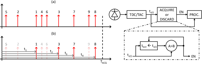
Figure 5: Example of SPAD response linearization with the acquire or discard acquisition method. In (a), each photon arrival time is represented by a red arrow and the order of arrival is indicated. The first run starts with the acquisition of photon #1, resulting in timestamp $t_{1}$. Photon #2 is discarded, since its arrival time is earlier than photon #1. The next recorded information comes instead from photon #3, which is later than photon #1, and sets the new minimum time. The run proceeds with the same criteria resulting in the stream of photon arrival times $t_{1}$, $t_{2}$, $t_{3}$ and $t_{4}$ from photons #1, #3, #7 and #8, which is a single realization of the emulated response of the linearized SPAD detector. On the right, a principle schematic is proposed, showing the lightweight usage of resources, with only one comparator and one register required on top of the processing circuit. The acquire or discard acquisition method is simple but inefficient, as most of the photons arrival times are discarded, resulting in longer acquisition times.

4.2 Acquisition scheme #2: Time-gated

The time-gated acquisition scheme works by delaying the activation of the SPAD to start from the previously acquired timestamp, until the end of the acquisition window is reached. With this approach, there is no need to discard timestamps, allowing for a faster acquisition. This, however, comes at the expense of a more complex hardware implementation, which needs a time-activated gating scheme, for instance using a programmable delay line. An example of acquisitions is shown in Figure 6, together with a possible implementation.

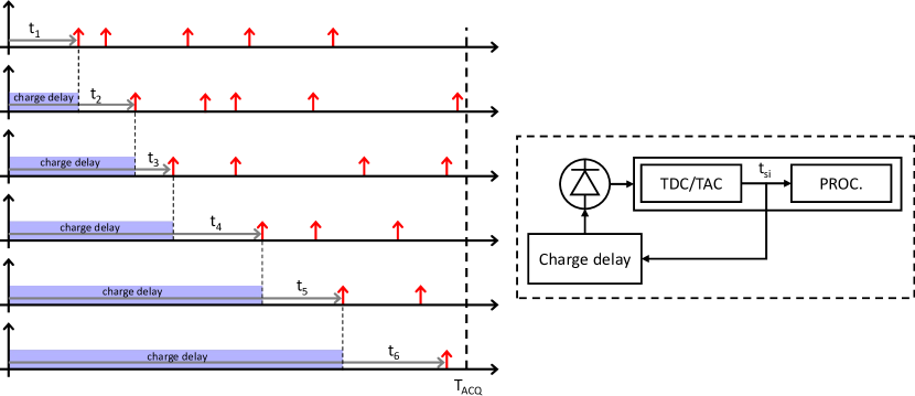
Figure 6: Example of SPAD response linearization with the time-gated acquisition method. With this approach, no photon timestamp is discarded thanks to the delayed activation of the SPAD for each timing measurement. During the charge delay phase, the SPAD front-end is forced OFF, thus photons can not be detected. For each measurement, the first timestamp is detected and used to increment either $N_{bg}$ or $N_{tot}$ and update the average time $\overline{t}_{tot}$. At the same time, the charge delay phase value is updated accordingly for the next measurement. As opposed to the acquire or discard method, more hardware resources are needed to build the delay element which controls the activation of the SPAD.

4.3 Mathematical description

While providing the same result, it is clear that the implementation cost and the performance of the two acquisition schemes are different. With the acquire or discard scheme, almost no hardware modification is required to an already existing SPAD sensor. However, because of the decimation process, the efficiency of the acquisition could be very low. This also depends on the intensity of the incoming flux of photons: the higher the intensity, the higher the probability to have smaller timestamps which block the detection process. On the other hand, the time-gated scheme requires a delay line and the SPAD-gating, but the efficiency is much higher since no decimation process occurs. To show the difference in terms of efficiency of the two proposed acquisition schemes, we run a Monte Carlo simulation with background light flux in the range $[10^{6},10^{8}]$ ph/s with the aim to linearize the SPAD response over an acquisition window $T_{acq}$ of 100 ns. As shown in Figure 7, at the highest flux of $10^{8}$ photons/sec, the amount of timestamps to be acquired to cover the acquisition window $T_{acq}$ for the acquire or discard scheme is more than 3 orders of magnitude higher compared to the more efficient time gated scheme. From the simulation, we can also identify the maximum number of measurements which can be executed by the two acquisition schemes to sustain an operation frame rate of 30 Frames Per Second (FPS). The time-gated scheme can average the linearized SPAD response up to $N=3\cdot 10^{4}$ times over the whole range of background light flux. On the other hand, with the same number $N$ of acquisitions, the acquire or discard scheme can only support up to $\approx 2.4\cdot 10^{7}$ ph/s of background flux.

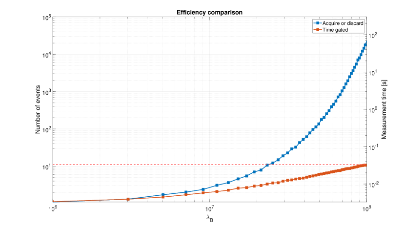
Figure 7: Result of Monte Carlo simulation comparing the two proposed acquisition schemes in terms of efficiency for increasing values of background light flux ($\lambda_{B}$) in the range $[10^{6},10^{8}]$ ph/s. On the left axis, we show the number of timestamps required to linearize the SPAD response over an acquisition window $T_{acq}$ of 100 ns. On the right axis, we show the total time required for the two methods to collect $N=3\cdot 10^{4}$ measurements, in order to average the linearized response of the SPAD N times. The horizontal line indicates a limit of $\approx 33.3$ ms, for an equivalent operation frame-rate of 30 FPS. With the time gated scheme, the required frame rate can be guaranteed over the entire range of background light flux, while considering the acquire or discard scheme, the maximum sustainable flux is limited to $\approx 2.4\cdot 10^{7}$ ph/s.

From a mathematical point of view, both acquisition methods allow sampling the correct distribution of the photon arrival times $(T_{n})_{n\geq 1}$. Let $T_{n}$ denote the occurrence time of the $n-$th event, i.e., the arrival of the $n$-th photon. This can be defined as the infimum of the set of times $t$ such that the number of arrivals $N_{t}$ in the interval $[0,t]$ is greater than or equal to $n$:

$$T_{n}:=\inf\{t\geq 0\,:\,N_{t}\geq n\},\qquad n\geq 1$$

By definition, $N_{T_{n}}=n$. We can therefore derive an equivalent representation of the random variables $T_{n}$. Indeed, for $n\geq 2$, the time $T_{n}$ of occurrence of the $n-$th event can be obtained as the infimum of the set of times $t$ greater than $T_{n-1}$ (the time of occurrence of the $(n-1)$-th event) such that the increment $N_{t}-N_{T_{n-1}}$, the number of events occurring in the interval $(T_{n-1},t]$, is greater than 1. Therefore

$$T_{1} :=\inf\{t\geq 0\,:\,N_{t}\geq 1\}$$

$$T_{n} :=\inf\{t\geq T_{n-1}\,:\,N_{t}-N_{T_{n-1}}\geq 1\},\quad n\geq 2$$

which corresponds to the results of the acquisition schemes described previously.

4.4 Comparison with state-of-the-art

In this section, we compare our histogram-less acquisition method with state-of-the-art SPAD-based LiDAR sensors in terms of memory requirement, scalability and tolerance to high background light flux. For all comparisons in this section, we consider for our method 16 bits of counters depth (i.e., up to 65535 counts for $N_{bg}$ and $N_{tot}$, respectively) and then 3 times the number of TDC bits (1xTDC bits required for the TDC word itself, and then 2xTDC bits to properly size the accumulator memory). First, we compare against standard sensors, i.e., sensors that require the raw timestamps to be read out to build the necessary histogram of timestamps off-chip. To provide a fair comparison, we do not consider the sensor resolution, which changes from chip to chip, but only the amount of memory required to build the histogram for one pixel. In the works we consider for our comparison [10, 15, 14, 13, 2], we extrapolate the total amount of per-pixel memory based on the number of reported TDC bits and on an 8-bit histogram depth for all of them. We then compare our solution to sensors that offer full on-chip histogram capability [36, 37, 33]. Also in this case, we consider the amount of memory reported in each work necessary to build the histogram of timestamps for one pixel. Results are reported in Figure 8, where an average memory reduction factor of $\approx 2129$ and $\approx 136$ for standard and full on-chip histogram sensors, respectively, is obtained. More comparison details, including minimum and maximum memory reduction factors are reported in Table 2.

Similarly to our method, partial histogram approaches [24, 25, 26, 31] are also quite effective in reducing the memory requirements. Nevertheless, our approach not only outperforms them with a memory reduction that ranges from 67% [25] to 3% [31], but also performs better in many other important aspects. In fact, unlike previous work, our approach does not have any of the following needs:

• The need to find the laser peak in time using a zooming or a sliding search procedure, which is at the basis of every partial histogram approach [32].

• The need to share hardware resources (TDCs, memory) among pixels in the same column [24] or in the same cluster [31], to reduce the area usage.

• The need for area consuming processors to manage the algorithm underlying the partial histogram technique and that can only be implemented using advanced 3D integrated technologies with single-pixel access [25].

All these translate into higher measurement time and laser power penalty as more acquisitions are needed than a standard full-histogram approach [32], and higher costs.

Our method, given the very limited amount of required memory resources, is also advantageous in terms of scalability to higher sensor resolutions, and also in terms of range extension. As an example, a standard histogram-based sensor with 15-bit TDC requires memory to store up to 32767 histogram bins per pixel. If the measurement range is doubled, the additional TDC bit results in an increase of 100% on the memory requirement. Conversely, with our approach, the amount of memory increase to double the range is limited to only $\approx$ 3.9%.

Concerning the tolerance to high background light flux, both detection processes can sustain very high flux regimes, with a limit determined by the finite resolution $T_{TS}$ of the timestamping circuit. This limit translates to the requirement $\frac{1}{\lambda_{B}+\lambda_{S}}\gg T_{TS}$, i.e., having a low probability that more than one photon fall into the same time bin. By considering a threshold on this probability, we can extract the maximum flux of photons $\lambda_{max}$ which can be sustained by our detection process. The probability to have more than one photon per time bin is expressed as $P(n>1)=1-e^{-\lambda_{max}\cdot T_{TS}}\cdot(1+\lambda_{max}\cdot T_{TS})$. By setting a threshold of less than 1%, and considering $T_{TS}=100$ ps, the maximum photon flux that can be sustained is equal to $\lambda_{max}\simeq 1.48\cdot 10^{9}$ ph/s. Compared to the maximum flux required by a standard system which must comply with the 5% rule, and with the hypothesis of an acquisition window $T_{acq}$ of 100 ns, our detection process can sustain a photon flux $\simeq$ 3000 times higher.

Table 2: Minimum, average and maximum memory reduction factor of the proposed histogram-less acquisition method against standard d-ToF sensors (off-chip histogram) [10, 15, 14, 13, 2] and sensors with on-chip full histogram capability [36, 37, 33].

Standard sensors				Full on-chip histogram
Min.	Avg.	Max.			Min.	Avg.	Max.
69.4 [2]	2129.5	6553.6 [13]			4.7 [33]	135.9	331.3 [36]

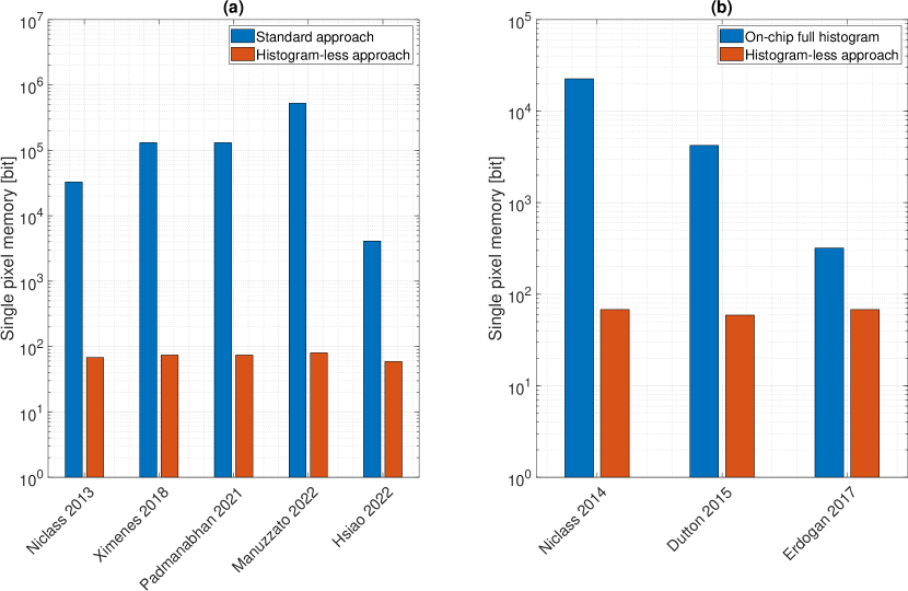
Figure 8: Comparison of the amount of per-pixel memory required by our histogram-less acquisition method against histogram-based d-ToF sensors. In (a), we consider standard sensors where every timestamp is read out and the histogram is built off-chip [10, 15, 14, 13, 2]. In (b), we consider sensors with full on-chip histogram capability [36, 37, 33].

5 Measurement results

The proposed acquisition scheme has been validated with measurements using real data from an existing single-point SPAD-based d-ToF sensor, with an architecture similar to the one from Perenzoni et al. [34], which in addition offers on-chip histogramming capability. The sensor is fabricated in a standard 150 nm CMOS process with the SPAD technology developed in the work by Xu et al. [38]. The histogram features 1024 bins with 10-b depth, and a TDC resolution of 100 ps. The SPADs are enabled synchronously with the beginning of the acquisition window and the first measured timestamp for each acquisition increments the corresponding histogram bin. After a user-selectable number of acquisitions, the histogram is read out and unpacked. Then, the unpacked data is shuffled to recover a realization vector of the arrival times of the detected photons.

Background events were generated by means of a $\approx$180 W fiber-coupled halogen illuminator pointed directly toward the sensor, while a black matte panel with low $\approx$10% reflectivity was selected as target, with a distance range from 1 m up to 3.8 m. A picture of the setup is shown in Figure 9, with indications on the main components.

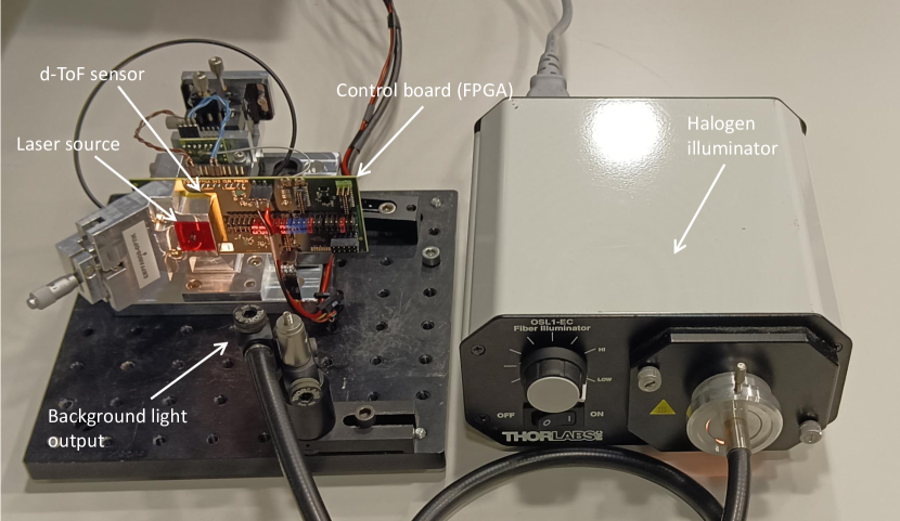
Figure 9: Measurement setup with the FPGA control board, d-ToF system and halogen illuminator for the generation of background light pointed directly toward the sensor.

First, we focus on the validation of the linearization behavior of the proposed acquisition scheme by considering only background light. Then, we consider the combination of background and laser together, as in a real scenario, and we compute the ToF with the proposed histogram-less acquisition scheme.

5.1 Preliminary considerations

As we base our measurements on the re-engineering of an existing d-ToF sensor, preliminary considerations are needed before providing further details on measurement results. The sensor measures the arrival time of the first detected photon for each laser pulse, as described in Section 2, which is stored in an on-chip histogram memory. Since the sensor measures the arrival time of the first photon, the statistical distribution is exponential, thus we are considering relative arrival times. A statistically valid realization of the incoming timestamps is obtained by unpacking and randomly shuffling the content of the histogram memory. The obtained realization is a vector of relative arrival times, which is the starting point of our measurement analysis.

In Section 4, we described two possible acquisition schemes. The acquire or discard scheme, even though is intrinsically inefficient, can be straightforwardly used with our dataset as it requires no hardware modification over the already existing SPAD-based d-ToF system. The time-gated scheme, while more efficient, requires a time-gating circuit which is not implemented in our sensor.

The first set of measurements focuses on background events only. In this case, there is a single source of events with intensity $\lambda_{B}$, so we can apply the time-gated scheme by computing the cumulative sums of timestamps to obtain absolute arrival times from relative ones. On the other hand, when events from background and laser are combined, as in a real measurement scenario, it is not possible to mimic the behavior of the time-gated scheme by means of the cumulative sum operation. In that case we rely on the acquire or discard scheme.

5.2 Measurements with background light only

We set the intensity of background light from a minimum of $\approx 6.5\cdot 10^{6}$ up to $\approx 133\cdot 10^{6}$ events/s. This is the rate of events at the output of the SPAD, which therefore takes into account all physical parameters of concern of a typical d-ToF system [35]. Considering an acquisition window of 100 ns, specific from the sensor [34], the equivalent average number of detections within $T_{acq}$ equals $\approx 0.65$ and $\approx 13.3$ for the minimum and maximum background light intensity, respectively. In both cases, this is much higher than the conventional limit of 5% events [18] (13 and 266 times higher, respectively), showing the high resistance of our method against pile-up distortion. By considering the equation which links the intensity of background events, $\lambda_{B}$, with the physical parameters of the system [35], it is possible to derive the equivalent background illumination level, in kilolux, up to a maximum of $\approx$ 85 kilolux. Measurement results are shown in Figure 10, showing a relative deviation from the reference background intensity extracted from the exponential fit of the original histogram of less than $\pm 0.5$ % over the whole range of values.

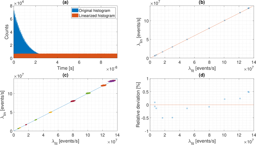
Figure 10: Linearization of the SPAD response with background events only. For each value of background flux, $8\cdot 10^{6}$ timestamps are acquired from the sensor. In (a), an example of linearized histogram is shown together with the original one (exponentially distributed) for a background flux of $\approx 100\cdot 10^{6}$ events/s. In (b), we show the flux of background events estimated from the linearized histogram of timestamps, $\lambda_{\textit{lin}}$ against the flux estimated from an exponential fit on the original histogram of timestamps, $\lambda_{\textit{fit}}$. In (c), for each value of background flux, the entire dataset was split in 200 subsets to analyze the homogeneity of the linearization process, while in (d), the relative deviation from the background flux measured from the original histograms is shown, used as a reference, demonstrating a relative deviation below $\pm 0.5$ % over all data subsets.

5.3 Measurements with background and laser light and extraction of the ToF

Our first goal is to show that the underestimation of background counts which occurs in a standard d-ToF system can be completely recovered with our acquisition scheme. This is demonstrated in the first measurement, displayed in Figure 11, which compares a traditional acquisition with the acquire or discard scheme, qualitatively showing the linearization process by means of the linearized histogram of timestamps.

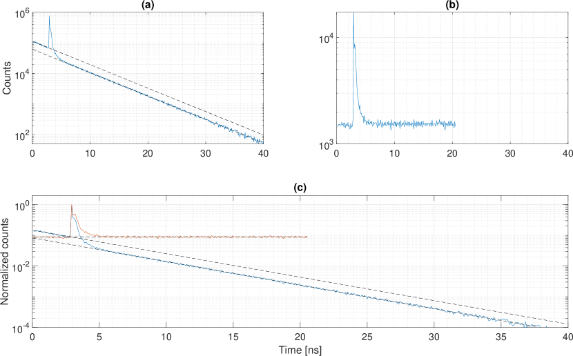
Figure 11: Qualitative measurement showing the linearization process of the proposed acquisition scheme. In (a), the original histogram of timestamps is shown in logarithmic scale, where the drop of counts which occurs after the laser peak is clearly visible. In (b), the histogram obtained with the acquire or discard scheme proves the efficacy of the linearization process, which fully compensates for the non-linearity of the detector. The length of the linearized histogram is shorter than the original dataset, as we decided to stop the linearization earlier to reduce the data loss which naturally occurs with the acquire or discard scheme. Due to the intrinsic inefficiency of this scheme, the histogram peak in (b) is attenuated by $\approx 34$ dB with respect to the original dataset in (a). In (c), the two histograms are shown together after normalization.

We then quantitatively evaluated the linearization process by estimating the intensity of background light from both portions of the histogram, i.e., before and after the laser peak. For this characterization, we used the $\approx$10% reflectivity target (black matte panel) at 2.5 m distance from the sensor. The results are depicted in Figure 12, showing a relative deviation from the ground truth (estimated from an exponential fit on the original dataset) below $\pm 4$ %.

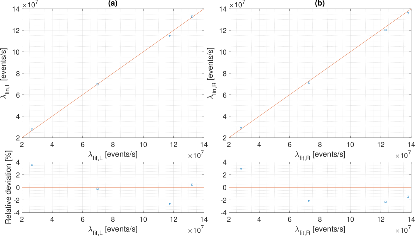
Figure 12: Quantitative characterization of the linearization process considering four different values of background flux, from $\approx 27.6\cdot 10^{6}$ events/s up to $\approx 133\cdot 10^{6}$ events/s with a target distance of 2.5 m. For each value of background flux, $2.5\cdot 10^{6}$ timestamps are acquired from the sensor. In (a), the relationship between the background fluxes computed before the laser peak is shown, where $\lambda_{\textit{fit},L}$ comes from an exponential fit on the original histogram, while $\lambda_{\textit{lin},L}$ comes from the linearized histogram. In (b), the same relationship is shown but considering the portion of background events after the histogram peak. For each portion, the relative deviation of the flux extracted from the linearized histogram of timestamps is shown, demonstrating an estimation error below $\pm 4$ % over the whole range. The application of the acquire or discard acquisition scheme results in a data reduction factor of $\approx 7.5$ and $\approx 165$ for the minimum and maximum background light flux, respectively.

In a different measurement, we verify the resistance of the proposed SPAD linearization method against pile-up distortion. To do so, we acquire several timestamps from the reflected laser pulse with a detection rate of 90%, which is 18 times higher than the conventional limit of 5%. The results, shown in Figure 13, proves the efficacy of our linearization method in challenging pile-up conditions where a standard sensor would fail. A reference measurement acquired with a conventional Time-Correlated Single Photon Counting (TCSPC) setup is shown as reference.

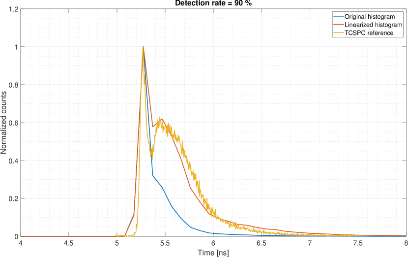
Figure 13: Characterization of the behavior of the proposed SPAD linearization method under strong pile-up conditions. The histogram obtained from the linearized vector of timestamps is compared against the original histogram (built from the detection of the first arrival time) and against a reference measurement obtained with a conventional TCSPC setup. In the histograms obtained from our sensor timestamps, the bin width is 100 ps, while the reference measurement from the TCSPC setup has 4 ps timing resolution. The proposed SPAD linearization method allows us to recover the full shape of the laser envelope even if the detection rate is 18 times higher than the conventional limit of 5%.

The last set of measurements shows the extracted ToF without the need to build a histogram of timestamps. For each measured distance, we run the linearization algorithm 250 times to have sufficient statistics to compute accuracy and precision. For each run of the algorithm, we average the results from $N=1.5\cdot 10^{4}$ vectors of linearized SPAD timestamps, to emulate an equivalent 30 FPS operation rate, as outlined in Section 4.3 and with Figure 7. For all measurements, the same $\simeq 10\%$ reflectivity target (black matte panel) was used, in the range from 1 m to 3.8 m, to emulate a challenging scenario for a typical SPAD-based d-ToF system. First, we evaluate the behavior of the ToF extraction process without background light. The results, depicted in Figure 14, show good agreement between the extracted ToF and the ground truth. Then, we repeat the measurements with the inclusion of background light by setting the halogen illuminator to generate a background light flux of $7.7\cdot 10^{6}$ events/s and $120\cdot 10^{6}$ events/s. The values of background light flux are considered at the output of the SPADs of the sensor, and they correspond to an illumination level of $\simeq$ 15 kilolux and $\simeq$ 75 kilolux, respectively. Results are shown in Figure 15 and 16, demonstrating the validity of the proposed histogram-less ToF estimation in a real setup.

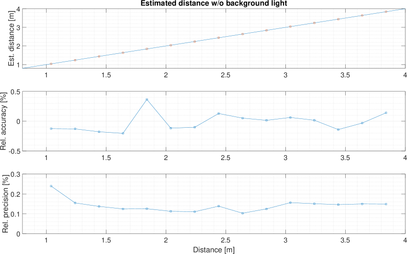
Figure 14: Measurement results with no background light, showing the ToF extracted without the need to build a histogram of timestamps. The relative accuracy is below $\pm 0.5\%$, while the relative precision is below $0.25\%$ for all measurements.

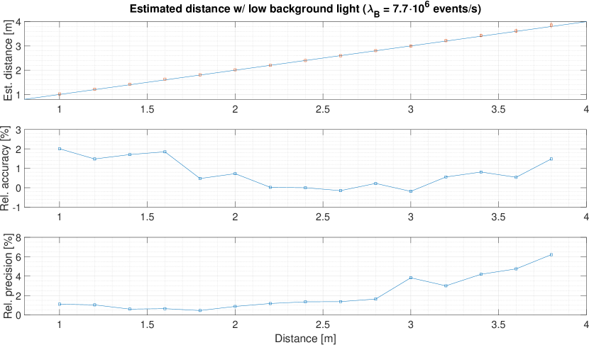
Figure 15: Measurement results with low background light flux ($\lambda_{B}=7.7\cdot 10^{6}$ events/s), showing the extracted ToF without the need to build a histogram of timestamps. The relative accuracy is in the range [-0.2,2] %, while the worst relative precision is $6\%$ at the highest distance of 3.8 m.

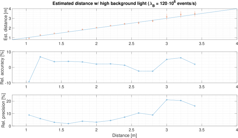
Figure 16: Measurement results with high background light flux ($\lambda_{B}=120\cdot 10^{6}$ events/s), showing the extracted ToF without the need to build a histogram of timestamps. The relative accuracy is in the range [-9,6.7] %, while the worst relative precision is $21\%$ at 3 m. With this high background light flux (corresponding to $\approx 75$ kilolux), and the decision to use a low reflectivity target ($\approx 10\%$), the maximum achieved range decreased to 3.4 m.

6 Conclusion

In this work, we demonstrate how to extract the time-of-flight information in a SPAD-based direct time-of-flight system without the need to build a resource and bandwidth-hungry histogram of timestamps. Moreover, the proposed method is resistant against high photon fluxes and can withstand detection rates three orders of magnitude higher than the conventionally recognized limit of 5%. The acquisition method, which is based on the linearization of the SPAD response, is suitable for integration in CMOS technology using low resources and is therefore scalable to large arrays, since it can be easily integrated per-pixel. The proposed extraction method has been completely characterized, first with Monte Carlo numerical simulations. The method is also mathematically justified, and we demonstrated its validity with real measurements, by repurposing an existing d-ToF sensor and using real data to extract the ToF. The proposed extraction method can be implemented at least in two ways, by means of the acquire or discard or time-gated detection schemes. While the acquire or discard scheme allows for the least usage of resources, it suffers from long integration times especially when the flux of photons is too high. On the other hand, the time-gated scheme can guarantee a more efficient acquisition at the expense of a per-pixel controllable delay element. Concerning the ToF extraction method, we demonstrated its validity by using an extremely low amount of resources, as only two counters and one accumulator are required.

Conflicts of interest

The authors declare no conflicts of interest.

References

- [1] V. Sesta, K. Pasquinelli, R. Federico, F. Zappa, and F. Villa, “Range-finding spad array with smart laser-spot tracking and tdc sharing for background suppression,” \JournalTitleIEEE Open Journal of the Solid-State Circuits Society 2, 26–37 (2022).
- [2] A.-T. Hsiao, C.-H. Liu, P.-H. Chen, Y.-L. Liu, W.-C. Wang, T.-H. Sang, C.-M. Tsai, G. Lin, J.-I. Guo, and S.-D. Lin, “Real-time lidar module with 64x128-pixel cmos spad array and 940-nm pcsel,” in 2022 IEEE Sensors Applications Symposium (SAS), (2022), pp. 1–6.
- [3] F. Villa, F. Severini, F. Madonini, and F. Zappa, “Spads and sipms arrays for long-range high-speed light detection and ranging (lidar),” \JournalTitleSensors 21 (2021).
- [4] K. Morimoto, A. Ardelean, M.-L. Wu, A. C. Ulku, I. M. Antolovic, C. Bruschini, and E. Charbon, “Megapixel time-gated spad image sensor for 2d and 3d imaging applications,” \JournalTitleOptica 7, 346–354 (2020).
- [5] Z.-P. Li, J.-T. Ye, X. Huang, P.-Y. Jiang, Y. Cao, Y. Hong, C. Yu, J. Zhang, Q. Zhang, C.-Z. Peng, F. Xu, and J.-W. Pan, “Single-photon imaging over 200 km,” \JournalTitleOptica 8, 344–349 (2021).
- [6] A. Tontini, L. Gasparini, L. Pancheri, and R. Passerone, “Design and characterization of a low-cost FPGA-based TDC,” \JournalTitleIEEE Transactions on Nuclear Science 65, 680–690 (2018).
- [7] J. Richardson, R. Walker, L. Grant, D. Stoppa, F. Borghetti, E. Charbon, M. Gersbach, and R. K. Henderson, “A 32×32 50ps resolution 10 bit time to digital converter array in 130nm cmos for time correlated imaging,” in 2009 IEEE Custom Integrated Circuits Conference, (2009), pp. 77–80.
- [8] V. Sesta, A. Incoronato, F. Madonini, and F. Villa, “Time-to-digital converters and histogram builders in spad arrays for pulsed-lidar,” \JournalTitleMeasurement 212, 112705 (2023).
- [9] I. Gyongy, N. A. W. Dutton, and R. K. Henderson, “Direct time-of-flight single-photon imaging,” \JournalTitleIEEE Transactions on Electron Devices 69, 2794–2805 (2022).
- [10] C. Niclass, M. Soga, H. Matsubara, S. Kato, and M. Kagami, “A 100-m range 10-frame/s 340 96-pixel time-of-flight depth sensor in 0.18- cmos,” \JournalTitleIEEE Journal of Solid-State Circuits 48, 559–572 (2013).
- [11] M. Perenzoni, D. Perenzoni, and D. Stoppa, “A 64 64-pixels digital silicon photomultiplier direct tof sensor with 100-mphotons/s/pixel background rejection and imaging/altimeter mode with 0.14km for spacecraft navigation and landing,” \JournalTitleIEEE Journal of Solid-State Circuits 52, 151–160 (2017).
- [12] K. Yoshioka, H. Kubota, T. Fukushima, S. Kondo, T. T. Ta, H. Okuni, K. Watanabe, M. Hirono, Y. Ojima, K. Kimura, S. Hosoda, Y. Ota, T. Koizumi, N. Kawabe, Y. Ishii, Y. Iwagami, S. Yagi, I. Fujisawa, N. Kano, T. Sugimoto, D. Kurose, N. Waki, Y. Higashi, T. Nakamura, Y. Nagashima, H. Ishii, A. Sai, and N. Matsumoto, “A 20-ch TDC/ADC hybrid architecture LiDAR SoC for 240 96 pixel 200-m range imaging with smart accumulation technique and residue quantizing SAR ADC,” \JournalTitleIEEE Journal of Solid-State Circuits 53, 3026–3038 (2018).
- [13] E. Manuzzato, A. Tontini, A. Seljak, and M. Perenzoni, “A -pixel flash lidar spad imager with distributed pixel-to-pixel correlation for background rejection, tunable automatic pixel sensitivity and first-last event detection strategies for space applications,” in 2022 IEEE International Solid- State Circuits Conference (ISSCC), vol. 65 (2022), pp. 96–98.
- [14] P. Padmanabhan, C. Zhang, M. Cazzaniga, B. Efe, A. R. Ximenes, M.-J. Lee, and E. Charbon, “7.4 a 256×128 3d-stacked (45nm) spad flash lidar with 7-level coincidence detection and progressive gating for 100m range and 10klux background light,” in 2021 IEEE International Solid- State Circuits Conference (ISSCC), vol. 64 (2021), pp. 111–113.
- [15] A. R. Ximenes, P. Padmanabhan, M.-J. Lee, Y. Yamashita, D. N. Yaung, and E. Charbon, “A 256×256 45/65nm 3d-stacked spad-based direct tof image sensor for lidar applications with optical polar modulation for up to 18.6db interference suppression,” in 2018 IEEE International Solid - State Circuits Conference - (ISSCC), (2018), pp. 96–98.
- [16] H. Seo, H. Yoon, D. Kim, J. Kim, S.-J. Kim, J.-H. Chun, and J. Choi, “Direct tof scanning lidar sensor with two-step multievent histogramming tdc and embedded interference filter,” \JournalTitleIEEE Journal of Solid-State Circuits 56, 1022–1035 (2021).
- [17] A. Tontini, L. Gasparini, and R. Passerone, “A SPAD-based linear sensor with in-pixel temporal pattern detection for interference and background rejection with smart readout scheme,” in Proceedings of the 2023 International Image Sensor Workshop, (Crieff, Scotland, UK, 2023).
- [18] W. Becker, “Advanced time-correlated single photon counting techniques,” \JournalTitleSpringer science & business media (2005).
- [19] J. Rapp, Y. Ma, R. M. A. Dawson, and V. K. Goyal, “High-flux single-photon lidar,” \JournalTitleOptica 8, 30–39 (2021).
- [20] I. Gyongy, S. W. Hutchings, A. Halimi, M. Tyler, S. Chan, F. Zhu, S. McLaughlin, R. K. Henderson, and J. Leach, “High-speed 3d sensing via hybrid-mode imaging and guided upsampling,” \JournalTitleOptica 7, 1253–1260 (2020).
- [21] A. Ruget, S. McLaughlin, R. K. Henderson, I. Gyongy, A. Halimi, and J. Leach, “Robust super-resolution depth imaging via a multi-feature fusion deep network,” \JournalTitleOpt. Express 29, 11917–11937 (2021).
- [22] S. Lindner, C. Zhang, I. M. Antolovic, M. Wolf, and E. Charbon, “A 252 × 144 spad pixel flash lidar with 1728 dual-clock 48.8 ps tdcs, integrated histogramming and 14.9-to-1 compression in 180nm cmos technology,” in 2018 IEEE Symposium on VLSI Circuits, (2018), pp. 69–70.
- [23] F. Mattioli Della Rocca, H. Mai, S. W. Hutchings, T. A. Abbas, K. Buckbee, A. Tsiamis, P. Lomax, I. Gyongy, N. A. W. Dutton, and R. K. Henderson, “A 128 × 128 SPAD Motion-Triggered Time-of-Flight Image Sensor With In-Pixel Histogram and Column-Parallel Vision Processor,” \JournalTitleIEEE Journal of Solid-State Circuits 55, 1762–1775 (2020).
- [24] C. Zhang, S. Lindner, I. M. Antolović, J. Mata Pavia, M. Wolf, and E. Charbon, “A 30-frames/s, spad flash lidar with 1728 dual-clock 48.8-ps tdcs, and pixel-wise integrated histogramming,” \JournalTitleIEEE Journal of Solid-State Circuits 54, 1137–1151 (2019).
- [25] S. W. Hutchings, N. Johnston, I. Gyongy, T. Al Abbas, N. A. W. Dutton, M. Tyler, S. Chan, J. Leach, and R. K. Henderson, “A reconfigurable 3-d-stacked spad imager with in-pixel histogramming for flash lidar or high-speed time-of-flight imaging,” \JournalTitleIEEE Journal of Solid-State Circuits 54, 2947–2956 (2019).
- [26] B. Kim, S. Park, J.-H. Chun, J. Choi, and S.-J. Kim, “7.2 a 48×40 13.5mm depth resolution flash lidar sensor with in-pixel zoom histogramming time-to-digital converter,” in 2021 IEEE International Solid- State Circuits Conference (ISSCC), vol. 64 (2021), pp. 108–110.
- [27] D. Stoppa, S. Abovyan, D. Furrer, R. Gancarz, T. Jessening, R. Kappel, M. Lueger, C. Mautner, I. Mills, D. Perenzoni, G. Roehrer, and P.-Y. Taloud, “A reconfigurable qvga/q3vga direct time-of-flight 3d imaging system with onchip depth-map computation in 45/40 nm 3d-stacked bsi spad cmos.” in Proc. Int. Image Sensor Workshop, 2021., (2021).
- [28] O. Kumagai, J. Ohmachi, M. Matsumura, S. Yagi, K. Tayu, K. Amagawa, T. Matsukawa, O. Ozawa, D. Hirono, Y. Shinozuka, R. Homma, K. Mahara, T. Ohyama, Y. Morita, S. Shimada, T. Ueno, A. Matsumoto, Y. Otake, T. Wakano, and T. Izawa, “7.3 a 189×600 back-illuminated stacked spad direct time-of-flight depth sensor for automotive lidar systems,” in 2021 IEEE International Solid- State Circuits Conference (ISSCC), vol. 64 (2021), pp. 110–112.
- [29] I. Gyongy, N. Dutton, H. Mai, F. Mattioli Della Rocca, and R. Henderson, “A 200kfps, 256 x 128 spad dtof sensor with peak tracking and smart readout.” in Proc. Ing. Image Sensor Workshop, 2021., (2021).
- [30] S. Park, B. Kim, J. Cho, J.-H. Chun, J. Choi, and S.-J. Kim, “An 80×60 flash LiDAR sensor with in-pixel histogramming TDC based on quaternary search and time-gated -intensity phase detection for 45m detectable range and background light cancellation,” in 2022 IEEE International Solid- State Circuits Conference (ISSCC), vol. 65 (2022), pp. 98–100.
- [31] C. Zhang, N. Zhang, Z. Ma, L. Wang, Y. Qin, J. Jia, and K. Zang, “A 240 × 160 3d-stacked spad dtof image sensor with rolling shutter and in-pixel histogram for mobile devices,” \JournalTitleIEEE Open Journal of the Solid-State Circuits Society 2, 3–11 (2022).
- [32] F. Taneski, T. A. Abbas, and R. K. Henderson, “Laser power efficiency of partial histogram direct time-of-flight lidar sensors,” \JournalTitleJournal of Lightwave Technology 40, 5884–5893 (2022).
- [33] A. T. Erdogan, R. Walker, N. Finlayson, N. Krstajic, G. O. S. Williams, and R. K. Henderson, “A 16.5 giga events/s 1024 × 8 spad line sensor with per-pixel zoomable 50ps-6.4ns/bin histogramming tdc,” in 2017 Symposium on VLSI Circuits, (2017), pp. C292–C293.
- [34] M. Perenzoni, N. Massari, L. Gasparini, M. M. Garcia, D. Perenzoni, and D. Stoppa, “A fast 50 × 40-pixels single-point DTOF SPAD sensor with photon counting and programmable ROI TDCs, with mm at 3 m up to 18 klux of background light,” \JournalTitleIEEE Solid-State Circuits Letters 3, 86–89 (2020).
- [35] A. Tontini, L. Gasparini, and M. Perenzoni, “Numerical model of spad-based direct time-of-flight flash lidar cmos image sensors,” \JournalTitleSensors 20 (2020).
- [36] C. Niclass, M. Soga, H. Matsubara, M. Ogawa, and M. Kagami, “A 0.18- m cmos soc for a 100-m-range 10-frame/s 200 96-pixel time-of-flight depth sensor,” \JournalTitleIEEE Journal of Solid-State Circuits 49, 315–330 (2014).
- [37] N. A. W. Dutton, S. Gnecchi, L. Parmesan, A. J. Holmes, B. Rae, L. A. Grant, and R. K. Henderson, “11.5 a time-correlated single-photon-counting sensor with 14gs/s histogramming time-to-digital converter,” in 2015 IEEE International Solid-State Circuits Conference - (ISSCC) Digest of Technical Papers, (2015), pp. 1–3.
- [38] H. Xu, L. Pancheri, G.-F. D. Betta, and D. Stoppa, “Design and characterization of a p/n-well spad array in 150nm cmos process,” \JournalTitleOpt. Express 25, 12765–12778 (2017).