Ising model on a Galton–Watson tree
with a sparse random external field

Abstract

We consider the Ising model on a supercritical Galton–Watson tree $\mathbf{T}_{n}$ of depth $n$ with a sparse random external field, given by a collection of i.i.d. Bernouilli random variables with vanishing parameter $p_{n}$. This may me viewed as a toy model for the Ising model on a configuration model with a few interfering external vertices carrying a plus spin: the question is to know how many (or how few) interfering vertices are enough to influence the whole graph. Our main result consists in providing a necessary and sufficient condition on the parameters $(p_{n})_{n\geqslant 0}$ for the root of $\mathbf{T}_{n}$ to remain magnetized in the large $n$ limit. Our model is closely related to the Ising model on a (random) pruned sub-tree $\mathbf{T}_{n}^{*}$ with plus boundary condition; one key result is that this pruned tree turns out to be an inhomogeneous, $n$-dependent, Branching Process. We then use standard tools such as tree recursions and non-linear capacities to study the Ising model on this sequence of Galton–Watson trees; one difficulty is that the offspring distributions of $\mathbf{T}_{n}^{*}$, in addition to vary along the generations $0\leqslant k\leqslant n-1$, also depend on $n$.
Keywords: Ising model, random graphs, random external field, phase transition.
MSC2020 AMS classification: Primary: 82B20, 60K35, 82B44, 82B26.

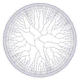
Figure 1: A tree of depth $n=15$ and its pruned version by a Bernoulli process on its leaves.

1 Introduction of the model and main results

The Ising model is a celebrated model, studied in depths for over 100 years. It was first introduced by Wilhelm Lenz and Ernst Ising as a model for magnetism, and was originally defined on regular lattices; we refer for instance to the books [4, 15] for a general introduction. Later, the Ising model was also studied on different types of graphs, starting with regular structures such as the Bethe lattice or Cayley tree, see [28] for an extensive summary on the subject. The seminal article [19], in which Lyons identifies the critical temperature of the model on an arbitrary infinite tree, opened the way to the study of the Ising model and other statistical mechanics models on tree-like graphs, and, more generally, on random graphs (see for instance [22]).

Motivated by the interest of the model to describe complex networks (see [13] for a review), the literature on the Ising model on random graphs has grown considerably in recent years. Let us mention a few relevant results on the subject. First, for the Ising model on quenched random graphs, the thermodynamic limit of has been studied in [10, 9, 11] as well as its critical behavior in [12, 17]. Thereafter, the annealed Ising model has also gotten some attention, see for instance [5, 6] references therein. More recently, the local weak limit of the Ising model on locally tree-like random graphs was considered in [1, 23].

However, most of the literature on the Ising model on random graphs considers free or plus boundary conditions or a homogeneous external field, but there does not seem to be many results when the boundary conditions or the external field are random (and depend on the size of the graph). In the present paper, we consider the Ising model on the simplest random graph possible, a Galton–Watson tree of depth $n$, but with a sparse random external field (which may be restricted to the boundary, which is close to being a boundary condition) whose distribution depends on $n$. We see our results as a first step towards the study of the Ising model on a random graph with a few external interfering vertices.

1.1 General setting of the paper

For a finite graph $G=(V,E)$, we consider the following Gibbs (ferromagnetic) Ising measure on spins $\sigma\in\{-1,+1\}^{|V|}$, with inverse temperature $\beta$ and external field $h=(h_{v})_{v\in V}$:

$$\mathrm{P}_{G,\beta}^{h}(\sigma):=\frac{1}{Z_{G,\beta}^{h}}\exp\bigg{(}\beta\Big{(}\sum_{\begin{subarray}{c}u,v\in V\\ u\sim v\end{subarray}}\sigma_{u}\sigma_{v}+\sum_{v\in V}h_{v}\sigma_{v}\Big{)}\bigg{)}\,,$$ (1.1)

where we denoted $u\sim v$ if $\{u,v\}\in E$. To simplify the statements and without loss of generality, we have assumed here that the coupling parameter is $J=1$.

In many cases, a natural boundary of $V$, denoted $\partial V\subset V$, can be identified. Then, we can consider the Ising model on the graph $G$ with boundary condition $\xi\in\{+1,-1\}^{\partial V}$ by considering the Gibbs measure

$$\mathrm{P}_{G,\beta}^{\xi}(\sigma):=\frac{1}{Z_{G,\beta}^{h}}\exp\bigg{(}\beta\Big{(}\sum_{\begin{subarray}{c}u,v\in V\setminus\partial V\\ u\sim v\end{subarray}}\sigma_{u}\sigma_{v}+\sum_{\begin{subarray}{c}u\in V\setminus\partial V,v\in\partial V\\ u\sim v\end{subarray}}\xi_{v}\sigma_{v}\Big{)}\bigg{)}\,.$$ (1.2)

For the Ising model with external field (1.1), in the case where $h_{v}=0$ for all $v\in V\setminus\partial V$, we will say that the Ising model has boundary external field.

Remark 1.1 (Exterior boundary).

It might also be natural to consider an exterior boundary of $G$, denoted $\partial^{\mathrm{ex}}G=(\partial^{\mathrm{ex}}V,\partial^{\mathrm{ex}}E)$, where $\partial^{\mathrm{ex}}V$ is a set of external vertices (disjoint from $V$) and $\partial^{\mathrm{ex}}E$ is a set of boundary edges $\{x,y\}$ with $x\in V$, $y\in\partial^{\mathrm{ex}}V$. We can then consider the Ising model on $G$ with exterior boundary condition $\xi\in\{-1,+1\}^{\partial^{\mathrm{ex}}V}$ by considering the Gibbs measure (1.2) on the graph $\bar{G}=(\bar{V},\bar{E})$ with $\bar{V}=V\cup\partial^{\mathrm{ex}}V$, $\bar{E}=E\cup\partial^{\mathrm{ex}}E$ and with boundary condition $\xi$ on $\partial\bar{V}=\partial^{\mathrm{ex}}V$.

Notice that, in the definition (1.1), if the external field has value $h_{v}\in\mathbb{Z}$, we may interpret the external field as some exterior boundary condition, where the set $\{v,h_{v}\neq 0\}$ can be interpreted as the boundary. Indeed, it corresponds to adding $|h_{v}|$ extra edges to $v$, all leading to vertices with assigned value $\mathrm{sign}(h_{v})$.

Setting of the paper.

In the following, we focus on the Ising model (1.1) with external field with $h_{v}\in\{0,1\}$; in fact, we will consider a random external field with either $(h_{v})_{v\in V}$ or $(h_{v})_{v\in\partial V}$ given by i.i.d. Bernoulli random variables of parameter $p\in(0,1)$. With an abuse of terminology, this corresponds to adding a plus (exterior) boundary condition to the vertices $v\in V$ with $h_{v}=+1$; it indeed corresponds to adding exactly one extra edge to $v$, with a plus on the other side of the edge. We refer to Figure 2 for an illustration.

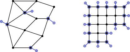
Figure 2: Representation of graphs with external fields $h_{v}\in\{0,1\}$. On each graph, we have circled the vertices where $h_{v}=+1$. The graph on the left has no natural boundary: we can think of the vertices with $h_{v}=+1$ as the boundary, each vertex being connected to a ‘$+$’ through an extra edge. On the right, the graph is a subset of $\mathbb{Z}^{2}$ and $h_{v}=+1$ for all $v\in\partial V$: this is our boundary external field and in the present case it does not exactly correspond to the Ising model with (exterior) plus boundary condition, because the corner vertices are connected to a ‘$+$’ through only one extra edge (to obtain plus boundary condition one should take $h_{v}=+2$ for the corner vertices).

One key physical quantity that we are going to study is the magnetization of a vertex $v\in V$:

$$\mathfrak{m}_{G,\beta}^{h}(v):=\mathrm{E}_{G,\beta}^{h}[\sigma_{v}]\,.$$

A closely related quantity is the probability that a given spin is in the plus state, namely $\mathrm{P}_{G,\beta}^{h}(\sigma_{v}=+1)=\frac{1}{2}(1+\mathfrak{m}_{G,\beta}^{h}(v))$ and the following log-likelihood ratio

$$r_{G,\beta}^{h}(v)=\log\bigg{(}\frac{\mathrm{P}_{G,\beta}^{h}(\sigma_{v}=+1)}{\mathrm{P}_{G,\beta}^{h}(\sigma_{v}=-1)}\bigg{)}=\log\bigg{(}\frac{1+\mathfrak{m}_{G,\beta}^{h}(v)}{1-\mathfrak{m}_{G,\beta}^{h}(v)}\bigg{)}\,.$$

Considering a sequence of growing graphs $(G_{n})_{n\geqslant 1}$ with associated non-negative external fields (that may depend on $n$), we say that there is spontaneous magnetization at inverse temperature $\beta$ if, choosing for each $n$ a vertex $v_{n}$ uniformly at random in the graph,the magnetization $\mathfrak{m}_{G_{n},\beta}^{h}(v_{n})$ (or equivalently the log-likelihood ratio $r_{G_{n},\beta}^{h}(v_{n}))$ remains bounded away from $0$ as $n\to\infty$ (either almost surely or in probability).

1.2 Ising model on the Configuration Model with interfering vertices

Let us now introduce one of our main motivation for considering a random sparse external field on a Galton–Watson tree: the Ising model on a random graph given by the configuration model, with a small proportion of additional interfering individuals.

The Configuration Model is a random graph in which edges are places randomly between vertices whose degrees are fixed beforehand. We refer to [29, Ch. 7] for a complete introduction but let us briefly present the construction. Let $N$ be the number of vertices of the graph, and let $\mathbf{d}=(d_{i})_{i\in\llbracket N\rrbracket}$ be a sequence of degrees, verifying $d_{i}\geqslant 1$; we also use the notation $\llbracket N\rrbracket=\{1,\ldots,N\}$. Then, the configuration model, noted $\mathrm{CM}_{N}(\mathbf{d})$ is an undirected random (multi)graph such that each vertex $i\in\llbracket N\rrbracket$ has degree $d_{i}$ (self-loops and multiple edges between pairs of vertices are allowed). It is constructed inductively as follows. As a preliminary to the construction, attach $d_{i}$ half-edges to each vertex vertex $i\in\llbracket N\rrbracket$, so that there is a collection $\mathcal{C}_{0}$ of $\ell_{N}:=\sum_{i=1}^{N}d_{i}$ available half-edges. Then, construct the first edge of the graph by choosing two half-edges uniformly at random from $\mathcal{C}_{0}$ and by pairing them; afterwards, remove these two half-edges from the set $\mathcal{C}_{0}$. After this first step, the new set $\mathcal{C}_{1}$ of available half-edges contains $\ell_{N}-2$ elements. This procedure is iterated $\frac{1}{2}\ell_{N}$ times, until there are no more half-edges available; notice that $\ell_{N}$ must be even.

Let us stress that the Configuration Model has no natural boundary, but one may think of having a few additional external vertices that are “interfering” with the graph. To model this, add $M_{N}$ vertices to the initial $N$ vertices of the model (we think of having $M_{N}\ll N$), all with degree $1$, and call these extra vertices interfering. One can then proceed to construct the graph as described above, i.e. a configuration model with both original and interfering vertices. Notice that, even if interfering vertices have degree one, an original vertex might have more than one interfering vertex attached to it. The $M_{N}$ interfering vertices may also be interpreted as some (external) boundary of the graph: in the context of the Ising model, one may consider the model where interfering vertices all have a plus spin, and try to determine a condition whether there is spontaneous magnetization on a sequence of configuration models, depending on $M_{N},N$ and the degree sequence $\mathbf{d}$.

In the case where $M_{N}\leqslant N$, another natural (and closely related) way of adding interfering external vertices is to consider the graph $\mathrm{CM}_{N}(\mathbf{d})$ and, to each vertex $i\in\llbracket N\rrbracket$, attach an extra (interfering) vertex of degree one, with probability $p_{N}:=M_{N}/N$. One obvious difference from the previous construction is that each vertex has at most one interfering vertex attached; also, in the first construction, interfering vertices change the distribution of the original configuration model. Indeed, an interfering vertex is taking over from an original one in the first construction, instead of just being added afterwards, as in the second construction. In the context of the Ising model, this version corresponds to having a (random) external field given by the spin of interfering vertices, say i.i.d. Bernoulli. Here again, one may ask whether there is spontaneous magnetization on a sequence of configuration models, depending on $p_{N},N$ and the degree sequence $\mathbf{d}$.

To summarize, the general question is to determine how many (or how few) interfering vertices are enough to have some influence on a random individual. Since the configuration model rooted at some randomly chosen vertex $o$ locally behaves like a branching process see [31, Sec. 4.2] (and also Section 1.5.4 below), we consider in the present paper, as a toy model, the Ising model on a Galton–Watson tree with randomly attached interfering vertices, i.e. a sparse external Bernoulli field.

1.3 Ising model on a Galton–Watson tree: main results

Let $\mu$ be a distribution on $\mathbb{N}$ and consider $\mathbf{T}_{n}$ a random tree of depth $n\in\mathbb{N}$ generated by a Branching Process with offspring distribution $\mu$, stopped at generation $n$; we will write $\mathbf{T}=\mathbf{T}_{n}$ if there is no confusion possible. We will denote by $\rho$ its root and by $\partial\mathbf{T}$ the set of its leaves. Also, we denote by $\mathbf{P}$ the law of $\mathbf{T}$, and we make the following assumption, which ensures in particular that the tree is super-critical.

Assumption 1.

The offspring distribution $\mu$ satisfy $\mu(0)=0$ and $\mu(1)<1$. In particular, $\nu:=\sum_{d=1}^{\infty}d\mu(d)>1$.

The condition $\mu(0)=0$ ensures that a.s. there is no extinction, so the tree $\mathbf{T}_{n}$ a.s. reaches depth $n$; additionally, it has no leaves except at generation $n$. We could weaken this assumption and work conditionally on having no extinction, using for instance [21, §5.7], but we work with Assumption 1 for technical simplicity.

We consider the Ising model (1.1) on a tree $\mathbf{T}$ with different possibilities for the external field or boundary condition:

• With ‘$+$’ boundary condition, meaning that $\sigma_{v}=+1$ (corresponding to an external field $h_{v}=+\infty$) if $v\in\partial\mathbf{T}$; the results are well-known since the work of Lyons [19], see Theorem 1.3 below. We denote the Ising Gibbs measure $\mathrm{P}_{n,\beta}^{+}$ in this case.

• With (sparse) Bernoulli external field, in which $(h_{v})_{v\in\mathbf{T}}$ are i.i.d. Bernoulli random with parameter $p_{n}$, independent of $\mathbf{T}$, whose law we denote by $\mathbb{P}$. We denote by $\mathrm{P}_{n,\beta}^{(p_{n})}$ the Ising Gibbs measure in this case.

• With (sparse) Bernoulli boundary external field, in which $(h_{v})_{v\in\mathbf{T}}$ are i.i.d. Bernoulli variables with parameter $\hat{p}_{n}:=p_{n}\mathds{1}_{\{v\in\partial\mathbf{T}\}}$; again, we denote their law by $\mathbb{P}$, by a slight abuse of notation. We denote by $\mathrm{P}_{n,\beta}^{(\hat{p}_{n})}$ the Ising Gibbs measure in this case.

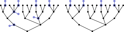
Figure 3: Two Ising models on a Galton–Watson tree with Bernoulli external field $h_{v}\in\{0,1\}$: the vertices with $h_{v}=+1$ are circle and a ‘$+$’ has been added to them. On the left, the external field $h_{v}\in\{0,1\}$ lives inside the whole tree (model $\mathrm{P}_{n,\beta}^{(p_{n})}$); on the right, the external field $h_{v}\in\{0,1\}$ lives only on the leaves (model $\mathrm{P}_{n,\beta}^{(\hat{p}_{n})}$).

Remark 1.2.

The second model (b) mimics the Ising model on a configuration model with sparse interfering vertices; the third model (c) is interesting in itself and will serve as a point of comparison. We stress that the parameter $p_{n}$ depends on the depth $n$ of the tree, but is constant among vertices in the tree (no matter their generation).

We then consider the root magnetization with external field (or boundary condition) $\mathrm{a}\in\{+,(p_{n}),(\hat{p}_{n})\}$:

$$\mathfrak{m}_{n,\beta}^{\mathrm{a}}:=\mathfrak{m}_{n,\beta}^{\mathrm{a}}(\rho):=\mathrm{E}_{n,\beta}^{\mathrm{a}}[\sigma_{\rho}]\,,$$ (1.3)

which is a random variable that depends on the realization of the tree $\mathbf{T}$ and of the field $(h_{v})_{v\in\mathbf{T}}$ (if the latter is random). We say that the root is asymptotically (positively) magnetized for the model $\mathrm{a}\in\{+,(p_{n}),(\hat{p}_{n})\}$ at inverse temperature $\beta$ if

$$\lim_{\varepsilon\downarrow 0}\liminf_{n\to\infty}\mathbf{P}\otimes\mathbb{P}\big{(}\mathfrak{m}_{n,\beta}^{\mathrm{a}}>\varepsilon\big{)}=1\,,$$ (1.4)

where $\mathbf{P}\otimes\mathbb{P}$ denotes the joint law of $\mathbf{T}$ and $(h_{v})_{v\in\mathbf{T}}$. Conversely, the root is asymptotically not magnetized if $\mathfrak{m}_{n,\beta}^{\mathrm{a}}$ goes to $0$ in $\mathbf{P}\otimes\mathbb{P}$-probability. Finally, note that these statements are equivalent if we replace the root magnetization by the log-likelihood ratio $r_{n,\beta}^{\mathrm{a}}:=r_{n,\beta}^{\mathrm{a}}(\rho)$ of the root.

Obviously, one can compare the three models (a), (b), (c) above, i.e. external field or boundary condition $\mathrm{a}\in\{+,(p_{n}),(\hat{p}_{n})\}$: indeed, we clearly have that $\mathfrak{m}_{n,\beta}^{+}\geqslant\mathfrak{m}_{n,\beta}^{(\hat{p}_{n})}$ and $\mathfrak{m}_{n,\beta}^{(p_{n})}\geqslant\mathfrak{m}_{n,\beta}^{(\hat{p}_{n})}$. We now state our main results.

(a) With a plus boundary condition on the leaves.

First of all, we recall the seminal result from Lyons [19] about the phase transition of the Ising model on a tree; we state here only in our simpler context of a Galton–Watson tree.

Theorem 1.3 ([19]).

Consider the Ising model on a Galton–Watson tree $\mathbf{T}$ with plus boundary condition. Then we have root asymptotic magnetization (1.4) (with $\mathrm{a}=+$) at inverse temperature $\beta$ if and only if $\nu\tanh(\beta)>1$, where we recall that $\nu$ is the mean offspring distribution.

The general result holds for a generic infinite tree $\mathbf{T}$: there is root magnetization if and only if $\mathrm{br}(\mathbf{T})\tanh(\beta)>1$, where $\mathrm{br}(\mathbf{T})$ is the branching number of the tree $\mathbf{T}$; we have $\mathrm{br}(\mathbf{T})=\nu$ for branching processes. In other words, Theorem 1.3 identifies the critical temperature for the Ising model on a tree: $\beta_{c}=\tanh^{-1}(\frac{1}{\nu})$.

(b) With a sparse Bernoulli external field inside the tree.

Let $(p_{n})_{n\geqslant 0}$ be a sequence of parameters in $[0,1]$. For each $n$, we let $\mathbf{T}_{n}$ be a GW tree up to generation $n$ and we let $(h_{v})_{v\in\mathbf{T}_{n}}$ be i.i.d. Bernoulli random variables of parameter $p_{n}$, independent of $\mathbf{T}_{n}$. Then, we have the following result, which is the main goal of this article.

Theorem 1.4.

Suppose that Assumption 1 holds and that $\mu$ has a finite second moment. Consider the Ising model on $\mathbf{T}$ with sparse Bernoulli external field, with $\lim_{n\to\infty}p_{n}=0$. Then we have asymptotic root magnetization (1.4) (with $\mathrm{a}=(p_{n})$) at inverse temperature $\beta$ if and only if

$$\nu\tanh(\beta)>1\qquad\text{ and }\qquad\liminf_{n\to\infty}(\nu\tanh(\beta))^{n}p_{n}>0\,.$$

In the case where $\liminf_{n\to\infty}p_{n}>0$, the root is asymptotically magnetized.

In other words, this theorem gives the exact speed at which $(p_{n})_{n\geqslant 0}$ should decrease in order not to have root magnetization. The first condition in the theorem comes from Lyons’ Theorem 1.3; the second condition shows that the sparsity of the Bernoulli field may somehow shift the critical point. For instance, if $p_{n}=\alpha^{n}$ for some $\alpha<1$, then one has root magnetization if and only if $\alpha\nu\tanh(\beta)\geqslant 1$, so the new critical inverse temperature is $\beta_{c}=\tanh^{-1}(\frac{1}{\alpha\nu})$; note that in that case, the root is also magnetized at the critical temperature, contrary to what happens in Theorem 1.3.

(c) With a sparse Bernoulli boundary external field on the leaves.

We have a similar result when we put the sparse Bernoulli field only on the leaves. As above, for each $n$, we let $\mathbf{T}_{n}$ be a GW tree up to generation $n$ and we let $(h_{v})_{v\in\mathbf{T}_{n}}$ be i.i.d. Bernoulli random variables of parameter $\hat{p}_{n}=p_{n}\mathds{1}_{\{v\in\mathbf{T}_{n}\}}$, independent of $\mathbf{T}_{n}$.

Theorem 1.5.

Suppose that Assumption 1 holds and that $\mu$ has a finite second moment. Consider the Ising model on $\mathbf{T}$ with sparse Bernoulli boundary external field , with $\lim_{n\to\infty}p_{n}=0$. Then we have asymptotic root magnetization (1.4) (with $\mathrm{a}=(\hat{p}_{n})$) at inverse temperature $\beta$ if and only if

$$\nu\tanh(\beta)>1\qquad\text{ and }\qquad\liminf_{n\to\infty}(\nu\tanh(\beta))^{n}p_{n}>0\,.$$

In the case where $\liminf_{n\to\infty}p_{n}>0$, the root is asymptotically magnetized if and only if $\nu\tanh(\beta)>1$.

Remark 1.6.

In Theorems 1.4-1.5, the second moment assumption on the offspring distribution is actually not needed to show that if $\nu\tanh(\beta)\leqslant 1$ or $\lim_{n\to\infty}(\nu\tanh(\beta))^{n}p_{n}=0$ then the root is asymptotically not magnetized.

Remark 1.7.

We could obviously consider a more general sparse random external field. For instance if $(h_{v})_{v\in\mathbf{T}}$ are i.i.d. with distribution $(1-p_{n})\delta_{0}+p_{n}\mu_{Y}$ for some positive random variable $Y$, one can easily compare this model with a Bernoulli external field and obtain identical results (provided that $\mathbb{E}[Y]<+\infty$). We have chosen to focus on Bernoulli external fields for the simplicity of exposition.

1.4 Outline of the proof and organisation of the paper

Let us outline our strategy of proof, which relies on standard tools for the Ising model on trees, namely Lyons’ iteration [19] for the log-likelihood ratio (we recall it in Section 2.2, see (2.5)), and Pemantle–Peres [27] relation between the log-likelihood ratio and the non-linear $3$-capacity of the tree, see Section 6.1 for an overview.

After a few preliminaries in Section 2, we prove in Section 3 the upper bound on the log-likelihood ratio and give the starting point of the proof of the lower bound. More precisely, in Section 3.1 we use Lyons’ iteration to derive an upper bound on the log-likelihood ratio of the root for the Ising model with Bernoulli external field inside the whole tree (which dominates the case where the external field is only on the leaves). The starting point of the lower bound is presented in Section 3.2: we show that the log-likelihood ratio of the root for the Ising model with Bernoulli boundary external field is equivalent to that of the Ising model with plus boundary external field on a modified tree, that we call pruned tree since it corresponds to removing all branches that do not lead to some $h_{v}=+1$. In other words, the Ising model with random (Bernoulli) boundary external field on $\mathbf{T}_{n}$ corresponds to an Ising model with plus boundary condition on a random subtree $\mathbf{T}_{n}^{*}$ of $\mathbf{T}_{n}$. Then, the rest of the paper consists in studying the Ising model with plus boundary condition on the pruned tree, that we denote $\mathbf{T}^{*}_{n}$.

First of all, in Section 4, we show that, under $\mathbf{P}\otimes\mathbb{P}$ the pruned tree is actually an inhomogeneous Branching Process, whose offspring distributions $(\mu_{k}^{*})_{0\leqslant k\leqslant n-1}$ are explicit (see (4.2)) and depend on the generation $k$ but also on the depth $n$ of the tree — in other words, we have a triangular array of offspring distributions.

Then, in Section 5 we show that the pruned tree somehow exhibits a sharp phase transition. More precisely, there exists some $k^{*}:=\log(p_{n}\nu^{n})/\log\nu$ (which depends on $n$ and go to $+\infty$ if $\liminf_{n\to\infty}p_{n}(\nu\tanh\beta)^{n}>0$), such that:

• if $k^{*}-k$ is large, then $\mu_{k}^{*}$ is very close to the original offspring distribution $\mu$;

• if $k-k^{*}$ is large, then $\mu_{k}^{*}$ is very close to being a Dirac mass at $1$.

This statement is made precise (and quantitative) in Proposition 5.7. Additionally, Section 5 contains several technical results quantifying this phase transition for various quantities of the pruned tree (for instance the mean and variances of $\mu_{k}^{*}$), that turn out to be important for the last part of the proof.

Finally, Section 6 concludes the proof of the lower bound on the log-likelihood ratio in Theorem 1.5 (which implies the lower bound in Theorem 1.4). Relying on the work of Pemantle–Peres [27], the log-likelihood ratio of the root for the Ising model on $\mathbf{T}^{*}_{n}$ with plus boundary condition is of the same order as the (non-linear) $L^{3}$- or $3$-capacity of $\mathbf{T}^{*}_{n}$, see Theorem 6.4. Hence, Section 6 focuses on estimating $\operatorname{Cap}_{3}(\mathbf{T}^{*}_{n})$; the estimates are collected in Proposition 6.5. Using that the $L^{3}$-capacity is bounded from below by the (linear) $2$-capacity, which coincide with the usual notion of conductance for resistor networks, Thomson’s principle enables us to obtain (after a few technical estimates) a lower bound for $\operatorname{Cap}_{3}(\mathbf{T}^{*}_{n})$, which concludes the proof. For the sake of completeness, we also provide in Proposition 6.5 an upper bound on $\operatorname{Cap}_{3}(\mathbf{T}^{*}_{n})$; in particular, we aim at giving a general scheme of proof to estimate the $L^{3}$-capacity of any inhomogeneous Galton–Watson tree. As a side result of independent interest, we find for instance that for the Ising model on a Galton–Watson tree (with offspring distribution of finite variance) with plus boundary condition, then at the critical temperature $\beta_{c}=\tanh^{-1}(\frac{1}{\nu})$ the magnetization of the root lies between $n^{-1}$ and $n^{-1/2}$, see Remark 6.7, which seems to be a new result (we believe that the correct order is $n^{-1/2}$, at least if the offspring distribution admits enough moments, but we leave this to another work since it is not the main focus of the paper).

1.5 Some further comments

Let us now conclude this section with several comments on our results, suggesting for instances possible directions for further investigations.

1.5.1 Comparison with a homogeneous but vanishing external field

A first natural question is to know whether the same results as in Theorems 1.4-1.5 would hold if one replaced the random Bernoulli external field $(h_{v})_{v\in\mathbf{T}}$ by its mean $(\mathbb{E}[h_{v}])_{v\in\mathbf{T}}$. This corresponds to considering the Ising model on a tree with a homogeneous but vanishing external field (either inside the whole tree or only on the boundary).

In particular, we want to look at the two following (sequences of) Ising models on the tree $\mathbf{T}$ of depth $n$: (i) homogeneous external field $h_{v}\equiv p_{n}$ for all $v\in\mathbf{T}$. (ii) homogeneous boundary external field $h_{v}\equiv p_{n}$ for all $v\in\partial\mathbf{T}$.

Using Lyons iteration as in Section 3.1 would yield that there is no root magnetization in the first model (hence in the second model) whenever $p_{n}\to 0$ and $p_{n}(\nu\tanh(\beta))^{n}\to 0$. We actually believe that if $p_{n}\to 0$ and $\liminf_{n\to\infty}p_{n}(\nu\tanh(\beta))^{n}>0$, then the root is asymptotically magnetized in the second model (hence in the first one). This does not appear straightforward, but one should be able to adapt our proof in Section 6 to derive such a result. Indeed in view of Lyons’ iteration (2.5), the model corresponds to some Ising model with plus boundary condition on some modified elongated tree $\tilde{\mathbf{T}}_{n}$, where $\tilde{\mathbf{T}}_{n}$ is obtained from $\mathbf{T}_{n}$ by adding “straight branches” of length $\ell$ to each leaf of $\mathbf{T}_{n}$ (with $\ell$ roughly chosen so that $\tanh(\beta)^{\ell}=p_{n}$), i.e. $\tilde{\mathbf{T}}_{n}$ is an inhomogeneous Branching Process of depth $n+\ell$ with offspring distribution $\mu_{k}=\mu$ for generations $k\leqslant n-1$ and $\mu_{k}=\delta_{1}$ for $n\leqslant k\leqslant n+\ell-1$. Then, thanks to Pemantle–Peres [27] comparison theorem, the problem is reduced to estimating the $3$-capacity of $\tilde{\mathbf{T}}_{n}$. For this, one may use a similar approach as in Section 6; in particular, we believe that the same estimates obtained for the $3$-capacity of our pruned tree $\mathbf{T}_{n}^{*}$ (cf. Proposition 6.5) hold for the elongated tree $\tilde{\mathbf{T}}_{n}$. we do not develop further on this issue since it is not the main purpose of our paper.

1.5.2 About the moment condition on the offspring distribution

Obviously, there are a few limitations on the generality of the offspring distribution $\mu$ that we consider on our Galton–Watson tree. The main restriction that we have is that $\mu$ admits a finite second moment. This assumption is useful when we estimate the effective resistance of the pruned tree $\mathbf{T}_{n}^{*}$ via a Thomson’s principle, see Section 6.2.2; in particular, by applying Markov’s inequality, we are reduced to estimating second moments of the size of the tree.

Adapting our proof to the case of an infinite variance (and possibly of an infinite mean) is an interesting question to consider. It is reasonable to expect that our main results remain valid in the case of an infinite variance, but this seems technically demanding; for instance one would need to control the tail of the random variables appearing in (6.11).

In the same spirit, another interesting question would be to obtain sharper bounds on the $3$-capacity of the pruned tree $\mathbf{T}^{*}_{n}$ (or even of $\mathbf{T}_{n}$), hence of the log-likelihood ratio of the root, for instance using a Thomson’s principle for the non-linear capacity. We believe that this improvement would for instance show that for the Ising model with plus boundary condition, at the critical temperature $\beta_{c}=\tanh^{-1}(1/\nu)$, the log-likelihood ratio (hence the magnetization) is of order $1/\sqrt{n}$, at least in the case where $\mu$ admits a finite third moment (since the $L^{3}$ Thomson principle should make third moments appear). What happens when the offspring distribution $\mu$ fails to have a third moment is an extremely interesting question.

1.5.3 Starting with an inhomogeneous, $n$-dependent, Galton–Watson tree

Keeping in mind our application to the Configuration Model (see Section 1.5.4 below), let us mention that our method appear to be robust to the case where the initial Galton–Watson tree $\mathbf{T}_{n}$ of depth $n$ is homogeneous but with an offspring distibution $\mu^{(n)}$ that depends on $n$. In particular, we believe that our results hold simply by replacing $\nu$ with $\nu^{(n)}$, the mean of the offspring distibution $\mu^{(n)}$, provided that the means $(\nu^{(n)})_{n\geqslant 0}$, resp.  the variances $(\sigma_{\mu^{(n)}}^{2})_{n\geqslant 0}$, remain bounded away from $1$, resp. $0$, and $+\infty$.

The case where one starts with a Galton–Watson tree $\mathbf{T}_{n}$ of depth $n$ which is inhomogeneous with offspring distribution $(\mu_{k}^{(n)})_{0\leqslant k\leqslant n-1}$ should be analogous. One would need to replace the quantity $\nu^{n}$ with $\prod_{k=0}^{n-1}\nu_{k}^{(n)}$, where $\nu_{k}^{(n)}$ is the mean of the offspring distibution $\mu^{(n)}_{k}$; again, one should for instance assume that the means $(\nu^{(n)}_{k})_{0\leqslant k\leqslant n-1,n\geqslant 1}$, resp. the variances $(\sigma_{\mu_{k}^{(n)}}^{2})_{0\leqslant k\leqslant n-1,n\geqslant 1}$, remain bounded away from $1$, resp. $0$, and $+\infty$.

1.5.4 Back to the configuration model

Coming back to the configuration model, we may try to use our toy model to make some predictions. Consider the configuration model recalled in Section 1.2, with $N$ vertices and degree sequence $\mathbf{d}=(d_{i})_{i\in\llbracket N\rrbracket}$. Denote $N_{k}:=|\{i\in\llbracket N\rrbracket,d_{i}=k\}|$ the number of vertices of degree $k$ and let $D_{N}$ be a random variable whose distribution is given by $\mathrm{P}(D_{N}=k)=N_{k}/N$, which corresponds to the degree of a vertex choosen uniformly at random. A standard and natural assumption on the model, see [31, § 1.3.3], is that, as $N\to\infty$, $D_{N}$ converges in distribution to some random variable $D$ and that we also have convergence of the first two moments of $D_{N}$ to those of $D$ (assuming that $\mathrm{E}[D^{2}]<+\infty$).

Then, it is known from [31, Thm. 4.1] that, choosing a vertex $o$ uniformly at random and rooting $\mathrm{CM}(\mathbf{d})$ at $o$, the rooted $\mathrm{CM}(\mathbf{d})$ locally converges (i.e. can be locally coupled with) to a branching process with offspring distribution $\mu$ (except the root which has offspring distribution $D$), where $\mu$ is the distribution of $D^{*}-1$, with $D^{*}$ is the size-biased of $D$; more precisely $\mu(k):=\frac{k+1}{\mathrm{E}[D]}\mathrm{P}(D=k+1)$.

Therefore, Assumption 1 corresponds to having $\mathrm{P}(D=1)=0$, $\mathrm{P}(D=2)<1$ and also $\nu:=\sum_{k=1}^{\infty}k\mu(k)=\frac{1}{\mathrm{E}[D]}\mathrm{E}[D(D-1)]>1$ (note that $\nu<+\infty$ if $\mathrm{E}[D^{2}]<+\infty$). The assumption that $\mu$ admits a finite second moment translates into the requirement that $\mathrm{E}[D^{3}]<+\infty$. Then, we can try to apply our results simply by analogy, i.e. identifying the configuration model rooted at a random vertex $v$ with a Galton–Watson tree $\mathbf{T}_{n}$ with offspring distribution $\mu$ (except at its root) and depth $n=\frac{1}{\log\nu}\log N$; the choice of $n$ is such that the number of vertices in $\mathbf{T}_{n}$ is roughly $\nu^{n}=N$. Our results then translate into the fact that the vertex $o$ is asymptotically magnetized if and only if $\liminf_{n\to\infty}p_{n}\nu^{n}\tanh(\beta)^{n}>0$, or since $p_{n}=M_{N}/N$, if and only if $\liminf_{N\to\infty}M_{N}N^{\alpha}>0$, where $\alpha:=\frac{1}{\log\nu}\log\tanh(\beta)$.

However, the approximation of the configuration model rooted at a random vertex $o$ with a Galton–Watson tree only works up to depth $\tilde{n}=c\log N$ for some constant $c>0$, provided that the maximal degree $d_{\mathrm{max}}=\max_{v\in\llbracket N\rrbracket}d_{v}$ verifies $d_{\rm max}=O(N^{a})$ for some $a<1$. This is a reformulation of [30, Lem. 3.3 and Rem. 3.4] in our context: a coupling can be made between the configuration model $\mathrm{CM}(\mathbf{d})$ rooted at a random vertex $o$ and a ($N$-dependent) Branching Process up to $m_{N}=o(\sqrt{N/d_{\rm max}})$ vertices; if $d_{\rm max}=N^{o(1)}$, this corresponds to a depth $\tilde{n}=\frac{1}{2\log\nu}\log N$ for the Galton–Watson tree. The fact that loops start to appear in the graph at some point breaks Lyons iteration’s argument and new ideas are needed. However, one should be able to obtain at least some bounds on the magnetization of $o$; in particular, the fact that our result is robust to the case of a $n$-dependent Galton–Watson tree could prove useful when working with the coupling mentioned above.

A natural (weak form of the) conjecture is the following.

Conjecture 1.

For the Ising model on the configuration model $\mathrm{CM}(\mathbf{d})$ with $M_{N}$ interfering external ‘$+$’ vertices, there exists some $\tilde{\alpha}>0$, depending only on the inverse temperature $\beta$ and the mean $\nu$, such that a randomly chosen vertex $o$ in $\mathrm{CM}(\mathbf{d})$ is:

• asymptotically magnetized if $M_{N}\geqslant N^{-\tilde{\alpha}+\varepsilon}$ for some $\varepsilon>0$;

• asymptotically not magnetized if $M_{N}\leqslant N^{-\tilde{\alpha}-\varepsilon}$ for some $\varepsilon>0$.

In other words, the threshold for having asymptotic root magnetization should be at a polynomial number of “interfering” vertices $M_{N}=N^{-\tilde{\alpha}+o(1)}$; it is natural to guess that $\tilde{\alpha}\leqslant\alpha$ with $\alpha:=\frac{1}{\log\nu}\log\tanh(\beta)$, but it is not clear whether $\tilde{\alpha}=\alpha$ or not, which is an interesting question.

1.5.5 About free boundary conditions and extremal Gibbs states

In the present paper, we focus on a non-negative (boundary) external field. Indeed, it is natural to consider such a condition to break the $+/-$ symmetry of the model.

Another setting, that has been extensively studied both in the physics and mathematics literature, is to consider the (nearest-neighbor, ferromagnetic) Ising model on an infinite tree with zero external field and free boundary condition. One question is then to determine whether the free measure $\mathrm{P}_{\beta}^{f}$ is equal to $\frac{1}{2}(\mathrm{P}_{\beta}^{+}+\mathrm{P}_{\beta}^{-})$, with $\mathrm{P}_{\beta}^{+}$, $\mathrm{P}_{\beta}^{-}$ the measures with ‘$+$’ and ‘$-$’ boundary conditions respectively. More generally, the question is to understand the set of extremal Gibbs measures (also called pure states), and in particular whether this set is reduced to $\mathrm{P}_{\beta}^{+}$, $\mathrm{P}_{\beta}^{-}$.

On a $k$-regular tree $\mathbb{T}_{k}$ (or more generally on hyperbolic graphs, see e.g. [33, 34]), it has been shown that at sufficiently low temperature, there are uncountably many extremal Gibbs states, see [18] and [2, 16] for rigorous results (we also refer to [8] for the case of other finite-spin models). In particular, there are multiple phase transitions; in this context, let us mention [24] which shows that the free Ising measure is a factor of IID beyond the uniqueness regime (see also [20] for a wider introduction to the problem).

It is then reasonable to ask whether the results on $k$-regular trees remain valid on random trees, or on tree-like graphs. As an example of such study, in [23], the authors consider the free Ising measure on a growing sequence of graphs $(G_{n})_{n\geqslant 1}$ that locally converge to a $k$-regular tree: their main result is that the Ising measure locally weakly converges to the mixture $\frac{1}{2}(\mathrm{P}_{\beta}^{+}+\mathrm{P}_{\beta}^{-})$. Our present work raises the natural question to determine whether (and to which point) this result continues to hold if one adds a signed sparse (boundary) random external field, i.e. if $(h_{v})_{v\in\mathbf{T}}$ (or $(h_{v})_{v\in\partial\mathbf{T}}$) are i.i.d. with law $\mathbb{P}(h_{v}=\pm 1)=\frac{1}{2}p_{n}$, $\mathbb{P}(h_{v}=0)=1-p_{n}$, with $\lim_{n\to\infty}p_{n}=0$. This is in fact related to the question of the effect of a random boundary condition on the Ising model (in particular on the coexistence of pure states), in the spirit of [32], see also [14] for a recent overview. We believe that such questions are natural and promising directions of research, in continuity of the present paper.

2 A few preliminaries

2.1 Some notation for trees

Let $\mathbf{t}=(V(\mathbf{t}),E(\mathbf{t}),\rho)$ be a tree with root $\rho$; with an abuse of notation, we also write $v\in\mathbf{t}$ as a shorthand for $v\in V(\mathbf{t})$. The distance between two vertices in the tree is the number of edges of the unique path connecting them.

Given two vertices $v,w\in\mathbf{t}$, we say that $w$ is a descendant of $v$, and we denote $v\leqslant w$, if the vertex $v$ is on the shortest path from the root $\rho$ to the vertex $w$. For a vertex $v\in\mathbf{t}$, we let $|v|$ denote the distance from $v$ to the root $\rho$; note that if we have $v\leqslant w$, we have $|v|\leqslant|w|$.

We consider a tree of depth $n$, that is such that $\max_{v\in\mathbf{t}}|v|=n$.

• We denote $t_{k}=\{v\in\mathbf{t}\;:\;|v|=k\}$ the $k$-th generation of the tree $\mathbf{t}$, for $k\leqslant n$.

• Given two vertices $v,w\in\mathbf{t}$ we say $w$ is a (direct) successor of $v$, and we note $v\rightarrow w$, if $v<w$ and $|v|=|w|-1$.

• For a vertex $v\in\mathbf{t}$, we denote $S(v)=\{w\in\mathbf{t}\;:\;v\rightarrow w\}$ the set of (direct) successors of $v$, and $d(v)=|S(v)|$ its cardinal, i.e. the number of descendants of $v$.

• We say that a vertex $v\in\mathbf{t}$ is a leaf if it has no successor, namely if $d(v)=0$, and we denote $\partial\mathbf{t}=\{v\in\mathbf{t},d(v)=0\}$ the set of leaves of the tree.

• For a vertex $v\in\mathbf{t}$, we let $\mathbf{t}(v)$ be the subtree of $\mathbf{t}$ consisting of $v$ (as a root) and all vertices $w$ such that $v\leqslant w$; if $v\in t_{k}$ is in generation $k$, we may also use the notation $\mathbf{t}_{k}(v)$ to make the dependence on $k$ explicit.

In the following, thanks to Assumption 1, we only consider trees that have no leaves except at generation $n$ ($\partial\mathbf{t}=t_{n}$), i.e. such that all vertices $|v|<n$ have at least one successor, $d(v)\geqslant 1$.

2.2 Log-likelihood ratio and Lyons iteration

One fundamental element of the proof of Theorem 1.3 is the fact that the log-likelihood ratio of the root magnetization can be expressed recursively on the tree. In this section, we introduce a few notation and state this recursive formula, that we call Lyons iteration; for the sake of completeness and because we adapt the iteration in the following, we recall how to obtain it.

Lyons iteration with plus boundary condition.

Let us start by giving the definition of the log-likelihood ratio $r_{\mathbf{t},\beta}^{+}(\rho)$ of the root on a tree $\mathbf{t}$ of depth $n$, with (classical) plus boundary conditions at temperature $\beta$:

$$r_{n,\beta}^{+}(\rho):=\log\bigg{(}\dfrac{\mathrm{P}_{n,\beta}^{+}(\sigma_{\rho}=+1)}{\mathrm{P}_{n,\beta}^{+}(\sigma_{\rho}=-1)}\bigg{)}$$

We also introduce the log-likelihood ratio $r_{n,\beta}^{+}(u)$ of a vertex $u\in\mathbf{t}$. We define the partition function of the Ising model on the sub-tree $\mathbf{t}(u)$ with plus boundary conditions at temperature $\beta$, conditioned on the vertex $u$ (the root of $\mathbf{t}(u)$) having spin $a\in\{-1,1\}$:

$$Z_{\beta}^{+,a}(u)=\sum_{\begin{subarray}{c}\sigma\in\{-1,1\}^{|\mathbf{t}(u)|}\\ \sigma_{u}=a\end{subarray}}\exp\bigg{(}\beta\Big{(}\sum_{\begin{subarray}{c}v,w\in\mathbf{t}(u)\\ v\sim w\end{subarray}}\sigma_{v}\sigma_{w}+\sum_{v\in\partial\mathbf{t}(u)}\sigma_{v}\Big{)}\bigg{)}\,.$$ (2.1)

Then, we let

$$r_{n,\beta}^{+}(u)=\log\bigg{(}\frac{Z_{\beta}^{+,+1}(u)}{Z_{\beta}^{+,-1}(u)}\bigg{)}\,,$$ (2.2)

which corresponds to the log-likelihood ratio of the root of the Ising model in the sub-tree $\mathbf{t}(u)$, of depth $n-|u|$, with plus boundary condition (we keep the subscript $n$ to remember that $u\in\mathbf{t}$ with $\mathbf{t}$ of depth $n$). Let us notice that, for any vertex $u\in\mathbf{t}$ different from the root, $r_{n,\beta}^{+}(u)$ does not correspond to $\log\big{(}\mathrm{P}_{n,\beta}^{+}(\sigma_{v}=+1)/\mathrm{P}_{n,\beta}^{+}(\sigma_{v}=-1)\big{)}$.

After a straightforward computation, for $u\in\mathbf{t}\setminus\partial\mathbf{t}$, we can write $(Z_{n,\beta}^{+,a}(u))_{a\in\{-1,+1\}}$ in terms of the partition functions $(Z_{n,\beta}^{+,a}(v))$ with $v$ successors of $u$: we have

$$Z_{\beta}^{+,a}(u)=\prod_{v,u\rightarrow v}\Big{(}e^{+\beta a}Z_{\beta}^{+,+1}(v)+e^{-\beta a}Z_{\beta}^{+,-1}(v)\Big{)}\,.$$ (2.3)

We can therefore express the log-likelihood ratio $r_{n,\beta}^{+}(u)$ in terms of partition functions:

$$r_{n,\beta}^{+}(u)=\log\bigg{(}\frac{Z_{\beta}^{+,+1}(u)}{Z_{\beta}^{+,-1}(u)}\bigg{)}=\sum_{u\to v}\log\bigg{(}\dfrac{e^{+\beta}Z_{n,\beta}^{+,+1}(v)+e^{-\beta}Z_{\beta}^{+,-1}(v)}{e^{-\beta}Z_{\beta}^{+,+1}(v)+e^{+\beta}Z_{\beta}^{+,-1}(v)}\bigg{)}\,.$$ (2.4)

Defining $g_{\beta}(x):=\log\Big{(}\frac{e^{2\beta}e^{x}+1}{e^{2\beta}+e^{x}}\Big{)}$, we therefore end up with the following crucial recursion:

$$r_{n,\beta}^{+}(u)=\begin{cases}\displaystyle\sum_{u\rightarrow v}g_{\beta}(r_{n,\beta}^{+}(v))&\qquad\text{if }u\notin\partial\mathbf{t}\,,\\ +\infty&\qquad\text{if }u\in\partial\mathbf{t}\,.\end{cases}$$ (2.5)

Lyons iteration with an external field.

We can also define, analogously to (2.2), the log-likelihood ratio of a vertex $u\in\mathbf{t}$ for the Ising model with external field $h=(h_{v})_{v\in\mathbf{t}}$.

For $u\in\mathbf{t}$, let $Z_{\beta}^{h,a}(u)$ denote the partition function of the Ising model on $\mathbf{t}(u)$ at temperature $\beta$ with external field $(h_{v})_{v\in\mathbf{t}(u)}$, conditioned on the root having spin $a\in\{-1,+1\}$. In the same way as in (2.3), we have for $u\in\mathbf{t}\setminus\partial\mathbf{t}$

$$Z_{\beta}^{h,a}(u)=e^{\beta h_{u}a}\prod_{v,\,u\rightarrow v}\Big{(}e^{+\beta a}Z_{\beta}^{h,+1}(v)+e^{-\beta a}Z_{\beta}^{h,-1}(v)\Big{)}\,.$$

Then, as in (2.4), the log-likelihood ratio $r_{n,\beta}^{h}(u)$ can be expressed in terms of the conditional partition functions, and we end up with the following recursion, analogous to (2.5):

$$r_{n,\beta}^{h}(u)=\begin{cases}\displaystyle 2\beta h_{u}+\sum_{u\to v}g_{\beta}(r_{n,\beta}^{h}(v))\quad&\text{if }u\notin\partial\mathbf{t}\,,\\ \displaystyle 2\beta h_{u}&\text{if }u\in\partial\mathbf{t}\,.\end{cases}$$ (2.6)

Here, we have also used that if $u\in\partial\mathbf{t}$ is a leaf, the log-likelihood ration $r_{n,\beta}^{h}(u)$ is easily seen to be $2\beta h_{u}$.

Remark 2.1.

Note that the Ising model on $\mathbf{t}$ with a plus boundary external field $h_{+}=(h_{v})_{v\in\partial\mathbf{t}}$, i.e. $h_{v}=+1$ for all $v\in\partial\mathbf{t}$, corresponds to the Ising model with plus boundary condition on some extended tree, obtained by adding an extra generation to $\mathbf{t}$ with exactly one descendant to all $v\in\partial\mathbf{t}$, recall Figure 2. In this setting, the log-likelihood ratios $r_{n,\beta}^{h_{+}}(u)$ verify the same recursion as in (2.5) but with a different initial condition on the leaves:

$$r_{n,\beta}^{h_{+}}(v)=2\beta\quad\text{if }v\in\partial\mathbf{t}\,.$$ (2.7)

2.3 The case of a non-vanishing sequence $(p_{n})_{n\geqslant 0}$

Before we move to the proofs, let us evacuate the case of a non vanishing sequence $(p_{n})_{n\geqslant 0}$ in the different models of Section 1.3.

Lemma 2.2.

Let $\mathbf{T}$ be a branching process satisfying Assumption 1 and consider the Ising model with sparse Bernoulli external field inside the tree, i.e. model (b) of Section 1.3, with parameters $(p_{n})_{n\geqslant 0}$ in $[0,1]$. If $\liminf_{n\to\infty}p_{n}>0$, then the root is asymptotically magnetized.

Proof.

To prove this, it is enough to consider the event where $h_{\rho}=+1$. On the event that $h_{\rho}=1$ and since we have $r_{n}^{(p_{n})}(v)\geqslant 0$ for all $v\leftarrow\rho$, we get that $r_{n}(\rho)\geqslant 2\beta$. Hence, for $\varepsilon<2\beta$ we have $\mathbf{P}\otimes\mathbb{P}(r_{n}(\rho)>\varepsilon)\geqslant\mathbb{P}(h_{\rho}=1)=p_{n}$. For such $\varepsilon$, we get that

$$\liminf_{n\to\infty}\mathbf{P}\otimes\mathbb{P}(r_{n}(\rho)>\varepsilon)>0\,,$$

which concludes the proof. ∎

In the case of the Ising model with non-vanishing Bernoulli boundary external field, i.e. model (c) of Section 1.3 with $\liminf_{n\to\infty}p_{n}>0$, one obtains a similar result as with plus boundary conditions, that is Theorem 1.3: the root is asymptotically magnetized if and only if $\nu\tanh(\beta)>1$. This is actually a corollary of Theorem 6.4 (from [27]) and our bounds on the $3$-capacity of the pruned tree, see Proposition 6.5 which is also valid for a non-vanishing sequence $(p_{n})_{n\geqslant 0}$.

3 Upper bound and main arguments for the lower bound

In the section, we consider the Ising model with sparse external field inside the tree, i.e. model (b) of Section 1.3. We let $(p_{n})_{n\geqslant 0}$ be a sequence in $[0,1]$ and we give an upper bound on the log-likelihood ratio and a lower bound in terms of an Ising model on a pruned tree with plus boundary external field.

3.1 Upper bound: Lyons argument

We show here the following proposition, using Lyons’ iteration (2.6), which gives a sufficient condition for having no root magnetization.

Proposition 3.1.

Suppose that Assumption 1 holds. Consider the Ising model on $\mathbf{T}$ with sparse Bernoulli external field, with $\lim_{n\to\infty}p_{n}=0$.

Then if $\lim_{n\to\infty}(\nu\tanh(\beta))^{n}p_{n}=0$, there is no asymptotic root magnetization. More precisely, there is a constant $C=C_{\beta,\nu}$ such that

$$\mathbf{E}\otimes\mathbb{E}\big{[}r_{n,\beta}^{p_{n}}(\rho)\big{]}\leqslant C\begin{cases}p_{n}&\quad\text{ if }\tanh(\beta)\nu<1\,,\\ \sqrt{p_{n}}&\quad\text{ if }\tanh(\beta)\nu=1\,,\\ p_{n}(\nu\tanh(\beta))^{n}&\quad\text{ if }\tanh(\beta)\nu>1\,.\end{cases}$$

Proof.

This is a simple application of the recursion formula (2.6). Let us first give a simple bound, valid for a generic tree $\mathbf{t}$ and external field $(h_{v})_{v\in\mathbf{t}}$.

Using the easy bound $g_{\beta}(x)\leqslant\tanh(\beta)x$ for all $x\geqslant 1$ (note that $\tanh(\beta)$ is the derivative of $g_{\beta}$ at $0$), we obtain from (2.6) that for any $u\in\mathbf{t}\setminus\partial\mathbf{t}$,

$$r_{n,\beta}^{h}(u)\leqslant 2\beta h_{u}+\tanh(\beta)\sum_{u\to v}r_{n,\beta}^{h}(v)\,.$$

Applying this inequality recursively we obtain the following upper bound for the log-likelihood ratio of the root $\rho$:

$$r_{n,\beta}^{h}(\rho)\leqslant\sum_{k=0}^{n}\tanh(\beta)^{k}\sum_{u\in t_{k}}2\beta h_{u}\,.$$

In our specific setting where $(h_{v})_{v\in\mathbf{T}}$ is an i.i.d. Bernoulli field with parameter $p_{n}$, we need to show that the upper bound goes to $0$ in $\mathbb{P}\otimes\mathbf{P}$ probability. We simply take its expectation with respect to $\mathbf{P}\otimes\mathbb{P}$: we obtain

$$\mathbf{E}\otimes\mathbb{E}\big{[}r_{n,\beta}^{(p_{n})}(\rho)\big{]}\leqslant 2\beta p_{n}\sum_{k=0}^{n}(\tanh(\beta)\nu)^{k}\,.$$ (3.1)

• In the case $\tanh(\beta)\nu<1$, the last sum is bounded by a constant and we have that $\mathbf{E}\otimes\mathbb{E}\big{[}r_{n,\beta}^{p_{n}}(\rho)\big{]}\leqslant cp_{n}$, which goes to $0$.

• In the case $\tanh(\beta)\nu>1$, we have

$$\mathbf{E}\otimes\mathbb{E}\big{[}r_{n,\beta}^{(p_{n})}(\rho)\big{]}\leqslant\frac{2\beta}{\tanh(\beta)-1}p_{n}((\tanh(\beta)\nu)^{n}-1)\leqslant c_{\beta,\nu}p_{n}(\tanh(\beta)\nu)^{n}\,,$$

which goes to $0$ under the assumptions of the proposition.

• The case $\tanh(\beta)\nu=1$ is a bit more subtle: taking the expectation in (3.1) gives the upper bound $\mathbf{E}\otimes\mathbb{E}[r_{n,\beta}^{(p_{n})}(\rho)]\leqslant 2\beta np_{n}$, which goes to $0$ only if $p_{n}=o(\frac{1}{n})$. In the general case, we need some extra work. Going back to Lyons’ iteration (2.6) and using that $x\mapsto g_{\beta}(x)$ is concave, we get by Jensen’s inequality (recalling that $\nu$ is the mean offspring distribution) that

$$\mathbf{E}\otimes\mathbb{E}\big{[}r_{n,\beta}^{(p_{n})}(u)\big{]}\leqslant 2\beta p_{n}+\nu g_{\beta}\Big{(}\mathbf{E}\otimes\mathbb{E}\big{[}r_{n,\beta}^{(p_{n})}(v)\big{]}\Big{)}\qquad\text{ for }u\notin\partial\mathbf{T}\,,$$

where $u,v$ are generic vertices at successive generations; note that the expectation $\mathbf{E}\otimes\mathbb{E}\big{[}r_{n,\beta}^{(p_{n})}(u)\big{]}$ depends only on (the distribution of) the subtree $\mathbf{t}(u)$ and $(h_{v})_{v\in\mathbf{t}(u)}$, so in fact only on $|u|$. Hence, setting $y_{k}:=\mathbf{E}\otimes\mathbb{E}[r_{n,\beta}^{(p_{n})}(u)]$ with $|u|=k$, we end up with the following iteration

$$y_{k}\leqslant\begin{cases}f_{n,\beta}(y_{k+1})\quad&\text{if }0\leqslant k<n\,,\\ 2\beta p_{n}&\text{if }k=n\,.\end{cases}$$ (3.2)

with $f_{n,\beta}(x)=2\beta p_{n}+\nu g_{\beta}(x)$, which is a concave increasing function. Let us denote $x_{n}$ the unique solution of $f_{n,\beta}(x_{n})=x_{n}$. Then, it is clear that either the initial condition verifies $y_{n}\leqslant x_{n}$ and then $y_{k}\leqslant x_{n}$ for all $k\leqslant n$, or it verifies $y_{n}>x_{n}$ and then $y_{k}\leqslant y_{n}=2\beta p_{n}$ for all $k\leqslant n$. We have therefore proven that

$$y_{0}=\mathbf{E}\otimes\mathbb{E}[r_{n,\beta}^{p_{n}}(\rho)]\leqslant\max\{2\beta p_{n},x_{n}\}\,,$$

and it remains to show that the fixed point $x_{n}$ goes to $0$ as $n\to\infty$. But this should be clear, since $x\mapsto\nu g_{\beta}(x)$ is a strictly concave function with slope $\nu\tanh(\beta)=1$ at the origin.

In fact, let us prove that $x_{n}=O(\sqrt{p_{n}})$. First, note that $\nu g_{\beta}(x)\leqslant x-c$ for any $x\geqslant 1$ with the constant $c=1-\nu g_{\beta}(1)>0$ (by concavity), so that $f_{n,\beta}(x)\leqslant 2\beta p_{n}+x-c$ for all $x\geqslant 1$. If $n$ is large enough so that $2\beta p_{n}<c$, this inequality cannot be verified at $x=x_{n}$, so we must have $x_{n}<1$. Then, writing that there is some constant $c_{\beta}>0$ such that $\nu g_{\beta}(x)\leqslant x-c_{\beta}x^{2}$ for all $x\in(0,1)$, we get that $x_{n}=f_{n,\beta}(x_{n})\leqslant 2\beta p_{n}+x_{n}-c_{\beta}x_{n}^{2}$ for all $n$ large enough. We conclude easily that $x_{n}\leqslant c^{\prime}_{\beta}\sqrt{p_{n}}$ for $n$ large, which is what was claimed. ∎

3.2 Lower bound: comparison with a pruned tree

First of all, we use the Ising model with Bernoulli boundary external field $(h_{v})_{v\in\partial\mathbf{T}}$, i.e. model (c) in Section 1.3, to get a lower bound for the magnetization of the Ising model with Bernoulli external field in the whole tree, since the magnetization is clearly higher in the second case.

Now, let us show in this section that, conditionally on the realization $\mathbf{t}$ of the Galton–Watson tree $\mathbf{T}$ and on the realization $h$ of a Bernoulli external field $(h_{v})_{v\in\partial\mathbf{T}}$, the magnetization is equal to the magnetization on a pruned (sub)-tree $\mathbf{t}^{*}$ with plus boundary external field $h_{+}=(h_{v})_{v\in\partial\mathbf{t}^{*}}$, i.e. with $h_{v}=+1$ for all $v\in\partial\mathbf{t}^{*}$. Informally, the pruned tree $\mathbf{t}^{*}$ is obtained by removing all branches in $\mathbf{t}$ that do not lead to a leaf with $h_{v}=+1$; we call this procedure the pruning of dead branches, see Figure 4 for an illustration.

To be more formal, given a tree $\mathbf{t}$ of depth $n$ and $(h_{v})_{v\in\partial\mathbf{t}}$ an external field with value in $\{0,1\}$, let us define indicator variables $(Y_{u})_{u\in\mathbf{t}}$ as follows:

$$Y_{u}=\begin{cases}+1&\quad\text{if there exists $v\geqslant u$, $v\in\partial\mathbf{t}$ such that $h_{v}=+1$}\\ 0&\quad\text{otherwise}\,.\end{cases}$$ (3.3)

We interpret having $Y_{u}=+1$ as the fact that the vertex $u$ belongs to a living branch, and so has “survived to the pruning”. Alternatively, we can construct $(Y_{u})_{u\in\mathbf{t}}$ iteratively starting from the leaves:

• for $v\in\partial\mathbf{t}=t_{n}$, set $X_{v}:=h_{v}$;

• iteratively, for $u\in\mathbf{t}\setminus\partial\mathbf{t}$, we set $Y_{u}=+1$ if and only if there is some $v\leftarrow u$ with $Y_{v}=+1$.

We then define the pruned tree as

$$\mathbf{t}^{*}=\mathrm{Pruned}_{h}(\mathbf{t}):=\{v\in\mathbf{t},Y_{v}=+1\}\,.$$ (3.4)

Figure 4: Illustration of the pruning procedure. On the left, we have represented the tree $\mathbf{t}$ and the leaves with $h_{v}=+1$ with dots. The picture on the right represents how the pruning procedure proceeds: in blue are all the “living branches” leading to a leaf with $h_{v}=+1$; in red are all the “dead branches” leading to $h_{v}=0$, that have to be pruned. The pruned tree $\mathbf{t}^{*}$ consists in keeping only the living (blue) branches.

Let us consider two following log-likelihood ratios, at inverse temperature $\beta$:

• For $u\in\mathbf{t}$, $r_{\mathbf{t},\beta}^{h}(u)$ is the log-likelihood ratio for the Ising model on $\mathbf{t}$ with external field $h\in\{0,1\}^{\partial\mathbf{t}}$ on the boundary;

• For $u\in\mathbf{t}^{*}$, $r_{\mathbf{t}^{*},\beta}^{h_{+}}(u)$ is the log-likelihood ratio for the Ising model on $\mathbf{t}^{*}$ with external field $h_{+}\equiv 1$ on the boundary $\partial\mathbf{t}$ (note that we have $h_{+}=h|_{\partial\mathbf{t}^{*}}$).

We now show the following lemma.

Lemma 3.2.

We have $r_{\mathbf{t},\beta}^{h}(u)=0$ for any $u\in\mathbf{t}\setminus\mathbf{t}^{*}$ and $r_{\mathbf{t},\beta}^{h}(u)=r_{\mathbf{t}^{*},\beta}^{h_{+}}(u)$ for any $u\in\mathbf{t}^{*}$. In particular, the log-likelihood ratio of the root verifies $r_{\mathbf{t},\beta}^{h}(\rho)=r_{\mathbf{t}^{*}}^{h_{+}}(\rho)$.

Proof.

We simply need to write the following Lyons recursions (see also Remark 1.1). On the tree $\mathbf{t}$, we have

$$r_{\mathbf{t},\beta}^{h}(u)=\begin{cases}\sum\limits_{u\rightarrow v}g_{\beta}\big{(}r_{\mathbf{t},\beta}^{h}(v)\big{)},&\qquad\text{if }u\notin\partial\textbf{t}\,,\\ 2\beta h_{v},&\qquad\text{if }v\in\partial\mathbf{t}\,.\end{cases}$$

Since $g_{\beta}(0)=0$, this readily proves that $r_{\mathbf{t},\beta}^{h}(u)=0$ if all $v\in\partial\mathbf{t}$ descendants of $u$ verify $h_{v}=0$, i.e. if $Y_{u}=0$ and $u$ has been pruned ($u\in\mathbf{t}\setminus bt^{*}$). On the tree $\mathbf{t}^{*}$, we have

$$r_{\mathbf{t}^{*},\beta}^{h_{+}}(u)=\begin{cases}\sum\limits_{u\rightarrow v}g_{\beta}\big{(}r_{\mathbf{t}^{*},\beta}^{h_{+}}(v)\big{)},&\qquad\text{if }v\notin\partial\textbf{t}^{*}\,,\\ 2\beta,&\qquad\text{if }v\in\partial\textbf{t}^{*}\,.\end{cases}$$

With a slight abuse of notation, we can extend the definition to the tree $\mathbf{t}$ by setting $r_{\mathbf{t}^{*},\beta}^{h_{+}}(u)=0$ if $u\in\mathbf{t}\setminus\mathbf{t}^{*}$. Now, this extended definition of $r_{\mathbf{t}^{*},\beta}^{h_{+}}$ yields exactly the same recursion as $r_{\mathbf{t},\beta}^{h}(u)$ so $r_{\mathbf{t}^{*},\beta}^{h_{+}}(u)=r_{\mathbf{t},\beta}^{h}(u)$ for all $u\in\mathbf{t}$. ∎

With Lemma 3.2, the rest of the paper then consist in studying the Ising model on the pruned version $\mathbf{T}^{*}_{n}$ of a Galton–Watson tree $\mathbf{T}_{n}$, with plus boundary external field. More precisely, we show the following.

Theorem 3.3.

Let $\mathbf{T}_{n}$ be a Galton–Watson tree of depth $n$ whose offspring distribution $\mu$ satisfies Assumption 1 and has a finite second moment, and let $(p_{n})_{n\geqslant 0}$ be a vanishing sequence. Let $\mathbf{T}^{*}_{n}$ be the pruned version of $\mathbf{T}_{n}$ with $(h_{v})_{v\in\partial\mathbf{T}}$ given by i.i.d. Bernoulli random variables with parameter $p_{n}$, i.e. $\mathbf{T}_{n}^{*}=\mathrm{Pruned}_{h}(T_{n}^{*})$. Then, for the Ising model on $\mathbf{T}_{n}^{*}$ with plus boundary external field on $\partial\mathbf{T}_{n}^{*}$, the root is asymptotically magnetized if and only if

$$\nu\tanh(\beta)>1\qquad\text{ and }\qquad\liminf_{n\to\infty}(\nu\tanh(\beta))^{n}p_{n}>0\,.$$

We proceed in several steps, which are split into the next three sections:

• First, we prove that, under $\mathbf{P}\otimes\mathbb{P}$, the pruned version of a Galton–Watson tree is an inhomogeneous branching process, whose distribution is explicit.

• Second, we study the shape of $\mathbf{T}_{n}^{*}$. More precisely, we observe that the pruned tree exhibits a sort of a phase transition: we identify some $k^{*}=k^{*}(\mu,p_{n})$ such that the pruned tree looks likes the original Galton–Watson tree up $k^{*}-O(1)$ and then looks like very thin branches from $k^{*}+O(1)$ to $n$.

• Lastly, we use our previous observation to estimate the (non-linear) $3$-capacity of $\mathbf{T}_{n}^{*}$, which is known to be related to the root magnetization, see [27].

4 Pruning the dead branches of a Galton–Watson tree

In this section, we consider $\mathbf{T}_{n}$ a random tree of depth $n\in\mathbb{N}$, generated by a branching process with offspring distribution $\mu$ such that $\mu(0)=0$. We let $p_{n}\in[0,1]$ be a given parameter and we let $\mathbf{T}^{*}_{n}$ be the pruned version of $\mathbf{T}$ with $(h_{v})_{v\in\partial\mathbf{T}}$ given by i.i.d. Bernoulli random variables with parameter $p_{n}$, as defined above in Section 3.2. Recall that we denote by $\mathbf{P}$ the law of $\mathbf{T}$ and by $\mathbb{P}$ the law of the i.i.d. Bernoulli random variables $(h_{v})_{v\in\partial\mathbf{T}}$.

The main result of this section is that $\mathbf{T}_{n}^{*}$, under $\mathbf{P}\otimes\mathbb{P}$, is a Branching Process with inhomogeneous $n$-dependent generation offspring distributions, that we denote $(\mu_{k}^{*})_{0\leqslant k\leqslant n-1}$. The fact that $\mathbf{T}^{*}_{n}$ is a branching process is a priori not obvious, since the pruning of a dead branch in the tree depends on random variables at the leaves.

4.1 Notation, statement of the result

Before we state the main result of this section, let us introduce some notation. For $k\in\{0,\ldots,n\}$, we denote $T_{k}$, respectively $T^{*}_{k}$, the $k$-th generation of $\mathbf{T}$, respectively $\mathbf{T}_{n}^{*}$.

We set, for $k\in\{0,\ldots,n\}$,

$$\gamma_{k}:=\mathbf{P}\otimes\mathbb{P}(Y_{u}=0)\quad\text{ for a generic }u\in T_{k}\,,\qquad\text{ and }\quad\delta_{k}:=1-\gamma_{k}\,,$$ (4.1)

where $Y_{u}=\mathds{1}_{\{u\in\mathbf{T}^{*}_{n}\}}$ is a Bernoulli random variable that indicates whether the vertex $u$ has survived the pruning, see (3.3).

Remark 4.1.

Here, $\gamma,\delta$ are indexed by their generations starting from the root (i.e. from the bottom of the tree to the top), but it is also helpful to index quantities by their distances to the leaves (i.e. from the top of the tree to the bottom). In the rest of the paper, we will denote with a bar quantities that are indexed by the distance to the leaves: for instance, for $k\in\{0,\ldots,n\}$, we set

$$\bar{\gamma}_{k}:=\gamma_{n-k}\,,\qquad\bar{\delta}_{k}=\delta_{n-k}=1-\bar{\gamma}_{k}\,.$$

Let $G$ be the generating function for the offspring distribution, that is

$$G(s):=\mathbf{E}[s^{X}]=\sum_{d=1}^{\infty}\mu(d)s^{d}\qquad s\in[0,1]\,,$$

where $X$ is a random variable of distribution $\mu$. Then, the parameters $\gamma_{k}$ can easily be expressed iteratively in terms of the generating function $G$.

Lemma 4.2.

The sequence $(\bar{\gamma}_{k})_{0\leqslant k\leqslant n}$ is characterized by the following iteration:

$$\bar{\gamma}_{0}=1-p_{n}\quad\text{ and for }k\in\{1,\ldots,n\}\,,\ \bar{\gamma}_{k}=G(\bar{\gamma}_{k-1})\,.$$

Equivalently, we have

$$\bar{\gamma}_{k}=\mathbf{E}\Big{[}(1-p_{n})^{|T_{k}|}\Big{]}\,.$$

Proof.

First of all, we have $\gamma_{n}=\mathbb{P}\otimes\mathbf{P}(Y_{v}=0)$ for $v$ a leaf, so by definition (3.3) of $Y_{v}$, we have $\gamma_{n}=\mathbb{P}(h_{v}=0)=1-p_{n}$, i.e. $\bar{\gamma}_{0}=1-p_{n}$.

Now, notice that for a generic $u\in T_{k}$ with $k<n$, by definition of $Y_{u}$ we have that $Y_{u}=0$ if and only if $Y_{u^{\prime}}=0$ for all $u^{\prime}\leftarrow u$. In other words, for a fixed realization of $\mathbf{T}$ we have

$$\mathbb{P}(Y_{u}=0)=\prod_{u^{\prime},u\rightarrow u^{\prime}}\mathbb{P}(Y_{u^{\prime}}=0),$$

since the variables $(h_{v})$ are independent on the different sub-trees $\mathbf{T}(u^{\prime})$, $u^{\prime}\leftarrow u$. Taking the expectation with respect to the tree and using the branching property we therefore get that for $k\leqslant n-1$,

$$\gamma_{k}=\mathbb{E}\big{[}(\gamma_{k+1})^{X}\big{]}=G(\gamma_{k+1})\,.$$

Using that $\bar{\gamma}_{k}=\gamma_{n-k}$, this gives the desired iteration.

For the other formula for $\bar{\gamma}_{k}$, we notice that $\bar{\gamma}_{k}=G^{\circ k}(1-p_{n})$, with $G^{\circ k}=G\circ\cdots\circ G$ ($k$ times). We obtain the desired formula since $G^{\circ k}$ is the generating function of $|T_{k}|$. ∎

We can now state our main result on the random pruned tree $\mathbf{T}_{n}^{*}$. For any $k\in\{0,\ldots,n\}$, define $\mu_{k}^{*}$ the distribution

$$\mu_{k}^{*}(d)=\dfrac{1}{\delta_{k}}\sum_{\ell\geqslant 0}\mu(d+\ell)\binom{d+\ell}{\ell}(\gamma_{k+1})^{\ell}(\delta_{k+1})^{d},\qquad d\in\mathbb{N}\,,$$ (4.2)

and note that $\mu_{k}^{*}$ also depends on $n$, through the parameters $\gamma$ and $\delta$ ( see Lemma 4.2).

Proposition 4.3.

The tree $\mathbf{T}^{*}_{n}=\mathrm{Pruned}_{h}(\mathbf{T}_{n})$ obtained by the pruning of the Galton–Watson tree $\mathbf{T}_{n}$ by i.i.d. Bernoulli random variables $(h_{v})_{v\in\partial\mathbf{T}}$ is, under $\mathbf{P}\otimes\mathbb{P}$, an inhomogeneous branching process. Its offspring distributions are $(\tilde{\mu}_{0}^{*},\mu^{*}_{1},\ldots,\mu_{n-1}^{*})$, where $\mu_{k}^{*}$ is defined in (4.2) above and $\tilde{\mu}_{0}^{*}(d)=\delta_{0}\mu_{0}^{*}(d)$ for $d\geqslant 1$, $\tilde{\mu}_{0}^{*}(0)=\gamma_{0}$.

4.2 Preliminary observations

Before we turn to the proof of Proposition 4.3, let us comment on the offspring distribution. First of all, $\tilde{\mu}_{0}^{*}(0)$ is the probability that the whole tree is pruned, i.e. $\gamma_{0}$, and $\mu_{0}^{*}$ is the law $\tilde{\mu}_{0}^{*}$ conditioned on being non-zero. Hence, conditionally on the whole tree not being pruned, $\mathbf{T}^{*}_{n}$ is an inhomogeneous branching process with offspring distribution $(\mu_{k}^{*})_{0\leqslant k\leqslant n-1}$.

We also have some nice interpretation of the distribution $\mu_{k}^{*}$. Conditionally on the tree not being pruned, we know that each vertex $u\in\mathbf{T}^{*}$ has at least one descendant in $\partial\mathbf{T}$ that has not been pruned; in other words, $\mu_{k}^{*}$ is supported on $\mathbb{N}$. It turns out that for $u\in T^{*}_{k}$, the number of children of vertex $u$ in $\mathbf{T}^{*}$ can be constructed as follows: take $X$ a random variable with distribution $\mu$, so $u$ has $X$ descendants in $\mathbf{T}$; prune these descendants with probability $\gamma_{k+1}$ independently, but conditionally on having at least one surviving descendant.

Definition 4.4.

Let $n\in\mathbb{N}$ and $p\in(0,1]$. A random variable $\hat{B}$ is said to follow a zero-truncated binomial of parameters $n$ and $p$, and we write $\hat{B}\sim\widehat{\operatorname{Bin}}(n,p)$ if

$$\mathrm{P}(\hat{B}=k)=\dfrac{1}{1-(1-p)^{n}}\binom{n}{k}p^{k}(1-p)^{n-k}\qquad k\in\{1,\ldots,n\}.$$

Put otherwise, we have $\mathrm{P}(\hat{B}=k)=\mathbb{P}(B=k\mid B>0)$ with $B\sim\operatorname{Bin}(n,p)$.

For a random variable $X$, we also write $W\sim\operatorname{Bin}(X,p)$ if for any $z\in\mathbb{N}$,

$$\mathrm{P}(W=z)=\sum_{d=1}^{\infty}\mathrm{P}(X=d)\mathrm{P}(B=z)\,,\quad\text{ with }B\sim\operatorname{Bin}(d,p)\,,$$

i.e. $W\sim\operatorname{Bin}(d,p)$ conditionally on $X=d$. A similar notation holds for $W\sim\widehat{\operatorname{Bin}}(X,p)$.

Lemma 4.5.

For all $k\in\{0,\ldots,n-1\}$, let $X_{k}^{*}$ be a random variable with law $\mu_{k}^{*}$. Then we have that $X_{k}^{*}\sim\widehat{\operatorname{Bin}}(X,\delta_{k+1})$, where $X$ is a random variable of distribution $\mu$. Put otherwise, if $B_{k}\sim\mathrm{Bin}(X,\delta_{k+1})$, then $\mathrm{P}(X_{k}^{*}=z)=\mathrm{P}(B_{k}=z\mid B_{k}>0)$ for $z\in\mathbb{N}$.

Proof.

For $k\in\{0,\ldots,n-1\}$, let $\tilde{X}_{k}\sim\widehat{\operatorname{Bin}}(X,\delta_{k+1})$. Letting $B_{k}\sim\operatorname{Bin}(X,\delta_{k+1})$, we have for $z\in\mathbb{N}$,

$$\mathrm{P}(\tilde{X}_{k}=z)=\mathrm{P}(B_{k}=z\mid B_{k}>0)=\dfrac{\mathrm{P}(B_{k}=z)}{1-\mathrm{P}(B_{k}=0)}\,,$$

with

$$\mathrm{P}(B_{k}=0)=\sum_{d=1}^{\infty}\mu(d)\mathrm{P}\big{(}\!\operatorname{Bin}(d,\delta_{k+1})=0\big{)}=\sum_{d=1}^{\infty}\mu(d)(1-\delta_{k+1})^{d}=\sum_{d=1}^{\infty}\mu(d)(\gamma_{k+1})^{d}.$$

Then $\mathrm{P}(B_{k}=0)=\mathbf{E}[(\gamma_{k+1})^{X}]=\gamma_{k}$, thanks to Lemma 4.2. Therefore, we end up with

$$\mathrm{P}(\tilde{X}_{k}=z)=\dfrac{1}{1-\gamma_{k}}\mathrm{P}(B_{k}=z)=\dfrac{1}{\delta_{k}}\sum_{d=1}^{\infty}\mu(d)\binom{d}{z}(\gamma_{k+1})^{d-z}(\delta_{k+1})^{z}=\mu_{k}^{*}(z),$$

which concludes the proof. ∎

4.3 Proof of Proposition 4.3

Our goal is to write $\mathbf{P}\otimes\mathbb{P}(\mathbf{T}^{*}_{n}=\mathbf{t}^{*})$ in terms of the offspring distributions $(\mu_{k}^{*})_{0\leqslant k\leqslant n-1}$. The approach for doing this is to consider all the possible trees $\mathbf{t}$ (sampled from $\mathbf{T}$) such that after pruning we may obtain $\mathbf{t}^{*}$.

First of all, notice that we clearly have $\mathbb{P}\otimes\mathbf{P}(\mathbf{T}^{*}_{n}=\emptyset)=\gamma_{0}$. Indeed, conditionally on the tree $\mathbf{T}_{n}$, the probability that the whole tree is pruned is $\mathbb{P}(h_{v}=0\,\forall\,v\in T_{n})=(1-p_{n})^{|T_{n}|}$, so $\mathbb{P}\otimes\mathbf{P}(\mathbf{T}^{*}_{n}=\emptyset)=\mathbf{E}[(1-p_{n})^{|T_{n}|}]=\gamma_{0}$, see Lemma 4.2.

We now work with $\mathbf{t}^{*}\neq\emptyset$ of depth $n$ and we write

$$\mathbb{P}\otimes\mathbf{P}(\mathbf{T}^{*}_{n}=\mathbf{t}^{*})=\sum_{\mathbf{t}\in\operatorname{BP}_{n}(\mu)}\mathbb{P}\otimes\mathbf{P}\big{(}\mathbf{T}=\mathbf{t},\mathrm{Pruned}_{h}(\mathbf{t})=\mathbf{t}^{*}\big{)}\,.$$

Here, $\operatorname{BP}_{n}(\mu)$ is the set of all trees $\mathbf{t}$ of depth $n$ generated by a Branching Process of offspring distribution $\mu$.

Preliminary calculation: offspring distribution. For $u\in\mathbf{T}_{n}$, we denote $X_{u}^{*}$ the number of descendants of $u$ inside the pruned tree $\mathbf{T}^{*}_{n}$. Notice that the number of successor of the vertex $u$ on the tree $\mathbf{T}_{n}$ (i.e. before pruning), that we denote $X_{u}$, has to verify $X_{u}\geqslant X_{u}^{*}$. We have

$$\{X^{*}_{u}=d\}=\bigcup_{\ell\geqslant 0}\bigcup_{V\subset S(u),|V|=\ell}\big{\{}X_{u}=d+\ell,Y_{v}=0\text{ for }v\in V,\ Y_{v}=1\text{ for }v\in S(u)\setminus V\big{\}}\,,$$

meaning that the vertex $u$ has $d+\ell$ successors (on $\mathbf{T}$) for some $\ell\geqslant 0$, and exactly $\ell$ of them get pruned.

Using this representation, we can compute the offspring distribution of a vertex $u$ at generation $k$. Using that vertices $v\leftarrow u$ in generation $k+1$ have a probability $\gamma_{k+1}$ of being pruned and that the events $\{Y_{v}=0\}_{v\leftarrow v}$ are independent (they depend on Bernoulli variables $(h_{v})$ in different sub-trees), we get for $d\geqslant 0$

$$\mathbb{P}\otimes\mathbf{P}(X^{*}_{u}=d)=\sum_{\ell\geqslant 0}\mu(d+\ell)\binom{d+\ell}{\ell}(\gamma_{k+1})^{\ell}(\delta_{k+1})^{d}\,.$$ (4.3)

Notice that (4.3) generalizes the iteration $\gamma_{k}:=\mathbb{P}\otimes\mathbf{P}(Y_{u}=0)=G(\gamma_{k+1})$ of Lemma 4.2.

Now, notice that conditionally on $\mathbf{T}_{n}^{*}\neq\emptyset$, a vertex $u\in\mathbf{T}^{*}_{n}$ has at least one descendant in $\mathbf{T}^{*}_{n}$. Note that we have $\mathbf{P}\otimes\mathbb{P}(X_{u}^{*}>0)=\mathbf{P}\otimes\mathbb{P}(Y_{u}=1)=\delta_{|u|}$, since $u$ has at least one descendant in the pruned tree if and only if it survives the pruning, i.e. $Y_{u}=1$. We therefore get the offspring distribution of a vertex $u\in T^{*}_{k}$ in $\mathbf{T}^{*}_{n}$ (conditioned on having $\mathbf{T}_{n}^{*}\neq\emptyset$):

$$\mathbf{P}\otimes\mathbb{P}(X^{*}_{u}=d\mid X_{u}^{*}>0)=\dfrac{1}{\delta_{k}}\sum_{\ell\geqslant 0}\mu(d+\ell)\binom{d+\ell}{\ell}(\gamma_{k+1})^{\ell}(\delta_{k+1})^{d}=\mu_{k}^{*}(d)\,.$$

It remains to show that the number of descendants in the different generations are independent.

Main calculation: probability of having a given pruned tree. Let $\mathbf{t}^{*}$ be a non-empty tree of depth $n$ which is a possible candidate for being a pruned version of a Galton–Watson tree $\mathbf{T}$. We let $d_{u}^{*}$ denote the number of descendants of $u\in\mathbf{t}^{*}$; recall that each vertex $u\in\mathbf{t}^{*}$ (in generation $k<n$) has to be such has it has at least one descendant, that is $d_{u}^{*}\geqslant 1$.

In order to have $\mathbf{T}^{*}_{n}=\mathbf{t}^{*}$, one must have $\mathbf{t}^{*}$ as a squeleton for $\mathbf{T}$, see Figure 5. Then, similarly as above, we can write the event $\{\mathbf{T}^{*}_{n}=\mathbf{t}^{*}\}$ as

$$\bigcap_{k=0}^{n-1}\bigcap_{u\in t_{k}^{*}}\bigcup_{\ell_{u}\geqslant 0}\bigcup_{V\subset S(u),|V|=\ell_{u}}\big{\{}X_{u}=d_{u}^{*}+\ell_{u},Y_{v}=0\text{ for }v\in V,\ Y_{v}=1\text{ for }v\in S(u)\setminus V\big{\}}\,,$$

meaning that each vertex $u\in\mathbf{t}^{*}$ must have $d_{u}^{*}+\ell_{u}$ successors in $\mathbf{T}$ for some $\ell_{u}\geqslant 0$, with exactly $\ell_{u}$ of them getting pruned; the descendants of $u$ inside $\mathbf{t}^{*}$ are the $v$ with $Y_{v}=1$.

Now, note that the events $\{Y_{v}=0\}$ in the above are all independent because they depend on different sub-trees of $\mathbf{T}$ (that lead to leaves with only $h\equiv 0$); recall that $\mathbf{P}\otimes\mathbb{P}(Y_{v}=0)=\gamma_{k+1}$ for $v\in T_{k}$. On the other hand, the events $\{Y_{v}=1\}$ are not independent, since all vertices $v\in\mathbf{T}$ such that $Y_{v}=1$ are ancestors of leaves with $h_{\cdot}=+1$. In particular, having $Y_{w}=1$ for a leaf $w\in\partial\mathbf{T}_{n}$ implies that $Y_{v}=1$ for all ancestors $v$ of $w$, see Figure 5. However, all the events $\{Y_{v}=1\}$ can be regrouped into a simpler event $\{h_{w}=1\,,\forall\,w\in t_{n}^{*}\}$, which is independent of all events $\{Y_{v}=0\}$; note that $\mathbf{P}\otimes\mathbb{P}(h_{w}=1\,,\forall\,w\in t_{n}^{*})=(p_{n})^{|t_{n}^{*}|}$.

All together, referring to Figure 5 for an illustration of the computation, and using also that the $(X_{v})_{v\in\mathbf{T}}$ are independent with distribution $\mu$, we obtain that

$$\mathbb{P}\otimes\mathbf{P}\big{(}\mathbf{T}^{*}_{n}=\mathbf{t}^{*}\big{)}=\prod_{k=0}^{n-1}\prod_{u\in t_{k}^{*}}\sum_{\ell_{u}\geqslant 0}\mu(d_{u}^{*}+\ell_{u})\binom{d_{u}^{*}+\ell_{u}}{\ell_{u}}(\gamma_{k+1})^{\ell_{u}}\times(p_{n})^{|t_{n}^{*}|}\,.$$ (4.4)

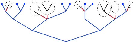
Figure 5: Illustration of the computation in (4.4): the tree $\mathbf{t}^{*}$ is represented in blue and the tree $\mathbf{T}$ whose pruned version is $\mathbf{t}^{*}$ is represented in black. For every $h_{w}=1$ in the leaves (represented by a blue dot), all the ancestors $v$ of $w$ automatically have $Y_{v}=1$: this contributes to (4.4) by a factor $(p_{n})^{|t_{n}^{*}|}$. A branch that is pruned just above generation $k$ contributes to the probability by a factor $\gamma_{k+1}$, and all these pruning events (represented by a red segment) are independent since they depend on distinct subtrees of $\mathbf{T}$ (the corresponding subtrees are circled with dashed lines).

We can now reformulate (4.4). Notice that $p_{n}=\delta_{n}$, and that $|t_{n}^{*}|=\sum_{u\in t_{n-1}^{*}}d_{u}^{*}$: we therefore get that $(p_{n})^{|t_{n}^{*}|}\prod_{u\in t_{n-1}^{*}}\sum_{\ell_{u}\geqslant 0}\mu(d_{u}^{*}+\ell_{u})\binom{d_{u}^{*}+\ell_{u}}{\ell_{u}}(\gamma_{k+1})^{\ell_{u}}$ is equal to

$$\prod_{u\in t_{n-1}^{*}}\sum_{\ell_{u}\geqslant 0}\mu(d_{u}^{*}+\ell_{u})\binom{d_{u}^{*}+\ell_{u}}{\ell_{u}}(\gamma_{k+1})^{\ell_{u}}(\delta_{n})^{d_{u}^{*}}=(\delta_{n-1})^{|t_{n-1}^{*}|}\prod_{u\in t_{n-1}^{*}}\mu_{n-1}^{*}(d_{u}^{*})\,,$$

where we have used the definition (4.2) of $\mu_{k}^{*}$ to get that $\sum_{\ell\geqslant 0}\mu(d+\ell)\binom{d+\ell}{\ell}(\gamma_{k+1})^{\ell}(\delta_{n})^{d}=\delta_{n-1}\mu_{n-1}^{*}(d)$. Similarly, we get that

$$(\delta_{n-1})^{|t_{n-1}^{*}|}\prod_{u\in t_{n-2}^{*}}\sum_{\ell_{u}\geqslant 0}\mu(d_{u}^{*}+\ell_{u})\binom{d_{u}^{*}+\ell_{u}}{\ell_{u}}(\gamma_{k+1})^{\ell_{u}}=(\delta_{n-2})^{|t_{n-2}^{*}|}\prod_{u\in t_{n-2}^{*}}\mu_{n-2}^{*}(d_{u}^{*}).$$

Therefore, iterating, we finally obtain from (4.4) that for any non-empty $\mathbf{t}^{*}$,

$$\mathbb{P}\otimes\mathbf{P}(\mathbf{T}^{*}_{n}=\mathbf{t}^{*})=\delta_{0}\prod_{k=0}^{n-1}\prod_{u\in t_{k}^{*}}\mu_{k}^{*}(d_{u}^{*})\,.$$

This concludes the proof since this gives that for any $\mathbf{t}^{*}$

$$\mathbb{P}\otimes\mathbf{P}(\mathbf{T}^{*}_{n}=\mathbf{t}^{*})=\tilde{\mu}_{0}^{*}(d_{\rho}^{*})\prod_{k=1}^{n-1}\prod_{u\in t_{k}^{*}}\mu_{k}^{*}(d_{u}^{*})=:\mathbf{P}^{*}(\mathbf{T}^{*}_{n}=\mathbf{t}^{*})\,,$$

where $\mathbf{P}^{*}$ is the law of some inhomogeneous branching process of depth $n$, with offspring distribution $(\tilde{\mu}^{*}_{0},\mu^{*}_{1},\ldots,\mu^{*}_{n})$. ∎

5 Transition in the shape of the pruned tree $\mathbf{T}^{*}_{n}$

5.1 Some notation and preliminaries

Recall that $X$ denotes a random variable with law $\mu$ and that $G(s):=\mathrm{E}[s^{X}]$ denotes its generating function. In all this section, we assume that $\mu(0)=0$, $\mu(1)<1$ and $\mu$ admits a finite second moment. For $k\geqslant 1$, we denote $m_{k}:=\mathrm{E}[X^{k}]\in(1,\infty]$ and we assume that $\nu:=m_{1}<+\infty$ and $m_{2}<+\infty$; we denote $\sigma^{2}=\mathrm{Var}(X)=m_{2}-m_{1}^{2}$. We also let

$$d_{0}:=\min\big{\{}d\geqslant 1,\mu(d)>0\big{\}}\qquad(d_{0}\geqslant 1)\,.$$

As the parameters $(\gamma_{k})_{0\leqslant k\leqslant n}$ are defined recursively in terms of the function $G$, see Lemma 4.2, let us state the following useful lemma on the function $G$, whose proof is elementary (we include it in Appendix A.1 for completeness).

Lemma 5.1.

We have the following bounds on $G$: for all $s\in[0,1]$,

$$1+m_{1}(s-1)\leqslant \,G(s)\leqslant 1+m_{1}(s-1)+C_{\mu}(s-1)^{2},$$ (5.1)

$$\mu(d_{0})s^{d_{0}}\leqslant \,G(s)\leqslant\mu(d_{0})s^{d_{0}}+s^{d_{0}+1},$$ (5.2)

where $C_{\mu}:=\frac{1}{2}(m_{2}-m_{1})$.

As a direct application of (5.1), we obtain the following bounds. For all $t\in[0,1]$,

$$\nu t(1-\tilde{C}_{\mu}t)\leqslant F(t):=1-G(1-t)\leqslant\nu t\,,$$ (5.3)

where $\tilde{C}_{\mu}=C_{\mu}/\nu$.

We also state the following lemma on recursively defined sequences $u_{j+1}=G(u_{j})$. Again, its proof is elementary but included in Appendix A.1 for completeness.

Lemma 5.2.

Let $\alpha\in(0,1)$ and $u_{0}\leqslant 1-\alpha$. Define recursively the sequence $(u_{j})_{j\geqslant 0}$ by the relation $u_{j+1}=G(u_{j})$. Then:

• If $d_{0}=1$, i.e. $\mu(1)\in(0,1)$, there is a constant $C_{\alpha}=C_{\alpha}(\mu)$ such that for all $j\geqslant 1$

  $$u_{0}\,\mu(1)^{j}\leqslant u_{j}\leqslant C_{\alpha}\,u_{0}\mu(1)^{j}.$$ (5.4)

• If $d_{0}\geqslant 2$, there is a constant $c_{\alpha}>0$ such that for all $j\geqslant 1$,

  $$(u_{0})^{d_{0}^{j-1}}\mu(d_{0})^{\frac{d_{0}^{j}}{d_{0}-1}}\leqslant u_{j}\leqslant e^{-c_{\alpha}d_{0}^{j}}\,.$$ (5.5)

(Note that the decay is doubly exponential in the second case.)

5.2 Some estimates on the parameters $(\gamma_{k})_{0\leqslant k\leqslant n}$

We now study how the parameters $(\gamma_{k})_{0\leqslant k\leqslant n}$ vary. Recall that $\gamma_{k}$ is defined in (4.1) as the probability that a vertex at generation $k$ is pruned, and also that we have set $\bar{\gamma}_{k}=\gamma_{n-k}$ and $\delta_{k}=1-\gamma_{k}$, $\bar{\delta}_{k}=\delta_{n-k}$.

Lemma 4.2 shows that $\bar{\gamma}_{k}$ is defined by the iteration $\bar{\gamma}_{k+1}=G(\bar{\gamma}_{k})$. Hence, we easily get that the parameters $(\bar{\delta}_{k})_{0\leqslant k\leqslant n}$ can be recursively determined in terms of the function $F(t):=1-G(1-t)$ in (5.3). Indeed, for $0\leqslant k\leqslant n$, we have

$$\bar{\delta}_{k+1}=1-\bar{\gamma}_{k+1}=1-G(\bar{\gamma}_{k})=1-G(1-\bar{\delta}_{k})=F(\bar{\delta}_{k})\,.$$

A first observation from these iterative definitions is that by convexity of $G$, and since $G(1)=1$, we get that $\bar{\gamma}_{k+1}=G(\bar{\gamma}_{k})\leqslant\bar{\gamma}_{k}$. We therefore have the following:

Lemma 5.3.

The sequence $(\gamma_{k})_{0\leqslant k\leqslant n}$ is non-decreasing; equivalently, $(\delta_{k})_{0\leqslant k\leqslant n}$ is non-increasing.

The main result of this section is that the parameters $(\gamma_{k})_{0\leqslant k\leqslant n}$, or equivalently $(\delta_{k})_{0\leqslant k\leqslant n}$, exhibit a (sharp) phase transition. Let us define:

$$k^{*}=k^{*}(p_{n}):=\log_{\nu}\big{(}p_{n}\nu^{n}\big{)}\,,\quad\text{ and }\quad\bar{k}^{*}=n-k^{*}=\log_{\nu}\Big{(}\frac{1}{p_{n}}\Big{)}\,,$$ (5.6)

where $\log_{\nu}(x)=\frac{1}{\log\nu}\log x$. In the following, we omit the integer part to simplify notation and often treat $k^{*},\bar{k}^{*}$ as integers. Let us note that $k^{*}\to\infty$ as soon as $p_{n}\nu^{n}\to\infty$ and that $\bar{k}^{*}\to\infty$ as soon as $p_{n}\to 0$.

Proposition 5.4.

There are constants $c_{1}\in(0,1)$ and $0<c_{2}\leqslant c_{3}$ (that depend only on the distribution $\mu$) such that:

$$\text{for all }k\geqslant k^{*}\qquad c_{1}\Big{(}\frac{1}{\nu}\Big{)}^{k-k^{*}}\leqslant\delta_{k}\leqslant\Big{(}\frac{1}{\nu}\Big{)}^{k-k^{*}}\,,$$

and, depending on whether $d_{0}=1$ (i.e. $\mu(1)\in(0,1)$) or $d_{0}\geqslant 2$,

$$\text{for all }k\leqslant k^{*}\qquad\left\{\begin{split}\text{if }d_{0}=1\,,\quad&\quad\ \ c_{2}\mu(1)^{k^{*}-k}\leqslant\gamma_{k}\leqslant c_{3}\mu(1)^{k^{*}-k}\,,\\ \text{if }d_{0}\geqslant 2\,,\quad&\quad\ e^{-c_{3}(d_{0})^{k^{*}-k}}\leqslant\gamma_{k}\leqslant e^{-c_{2}(d_{0})^{k^{*}-k}}\,.\end{split}\right.$$

The lower bounds in the above are not particularly relevant to our purpose (they however have some technical use in the proofs), so let us write more compactly (whether $d_{0}=1$ or $d_{0}\geqslant 2$) upper bounds that we will use repeatedly in the proof. There is a constant $c_{4}>0$ such that

$$\gamma_{k}\leqslant e^{-c_{4}(k^{*}-k)}\quad\text{for }k\leqslant k^{*}\qquad\text{ and }\qquad\delta_{k}\leqslant\Big{(}\frac{1}{\nu}\Big{)}^{k-k^{*}}\quad\text{for }k\geqslant k^{*}\,.$$ (5.7)

The interpretation of Proposition 5.4 (or of (5.7)) is as follows. On one hand, when $k$ is much smaller than $k^{*}$ in the sense that $k^{*}-k\gg 1$, then $\gamma_{k}$ is very small (or $\delta_{k}$ is close to $1$), meaning that vertices have an exponentially small chance of being pruned. On the other hand, when $k$ is much larger than $k^{*}$ in the sense that $k-k^{*}\gg 1$, then $\delta_{k}$ is very small (or $\gamma_{k}$ is close to $1$), meaning that vertices are very likely being pruned. The transition is sharp, in the sense that it occurs in a window of size $O(1)$.

One may therefore have the following picture in mind for the pruned tree $\mathbf{T}_{n}^{*}$: for $k\leqslant k^{*}$, $\mathbf{T}_{n}^{*}$ resembles the original Galton–Watson tree, while for $k\geqslant k^{*}$, $\mathbf{T}_{n}^{*}$ has thin long branches (i.e. with only one descendant per vertex) recalling that the vertices of the pruned tree are conditioned on having at least one descendant. This picture is made more formal in Proposition 5.7 below, see also Figure 1 on page 1 for an illustration.

Remark 5.5.

In the case where $p_{n}=\alpha^{n}$ with $\alpha\in(0,1)$, then we have that $\bar{k}^{*}=n\log_{\nu}(\frac{1}{\alpha})$ with $\eta_{\alpha}:=\log_{\nu}(\frac{1}{\alpha})\in(0,1)$. This shows that the transition occurs sharply around generation $k^{*}=(1-\eta_{\alpha})n$.

Proof of Proposition 5.4.

For our purposes, it will be more convenient to work with the iteration from Lemma 4.2 which goes from the leaves to the root. We therefore prefer to work with $\bar{\gamma}_{k},\bar{\delta}_{k}$ instead of $\gamma_{k},\delta_{k}$, and we want to show the following:

$$\frac{c_{1}}{(\nu)^{\bar{k}^{*}-k}} \leqslant\bar{\delta}_{k}\leqslant\frac{1}{(\nu)^{\bar{k}^{*}-k}} \text{for all }k\leqslant\bar{k}^{*},$$

$$c_{2}\mu(1)^{k-\bar{k}^{*}} \leqslant\bar{\gamma}_{k}\leqslant c_{3}\mu(1)^{k-\bar{k}^{*}} \text{for all }k\geqslant\bar{k}^{*}\,.$$

The second line being valid if $d_{0}=1$ (i.e. $\mu(1)\in(0,1)$), and replaced with

$$e^{-c_{3}(d_{0})^{k-\bar{k}^{*}}}\leqslant\bar{\gamma}_{k}\leqslant e^{-c_{2}(d_{0})^{k-\bar{k}^{*}}}$$

in the case where $d_{0}\geqslant 2$. The main idea of the proof is to use the iteration $\bar{\delta}_{k+1}=F(\bar{\delta}_{k})$ together with the estimate (5.3), until $\bar{\delta}_{k}$ is not small enough; we show that this occurs around $k=\bar{k}^{*}$. Then, we apply Lemma 5.2 to the iteration $\bar{\gamma}_{k+1}=G(\bar{\gamma}_{k})$ starting from $k=\bar{k}^{*}$ for which $\bar{\gamma}_{\bar{k}^{*}}$ is not too small.

Step 1. We start with some intermediate result which makes use of (5.3).

Lemma 5.6.

Let $\bar{k}_{1}^{*}=\min\{0\leqslant k\leqslant n\,:\,\sum_{i=0}^{k}\tilde{C}_{\mu}\bar{\delta}_{i}>1/2\}$, with $\tilde{C}_{\mu}$ as in (5.3). Then, for all $k\leqslant\bar{k}_{1}^{*}$ we have

$$\dfrac{1}{2}(\nu)^{k}p_{n}\leqslant\bar{\delta}_{k}\leqslant(\nu)^{k}p_{n}.$$ (5.8)

The upper bound is valid for any $0\leqslant k\leqslant n$.

Proof.

Let $0\leqslant k\leqslant n$. As $\bar{\delta}_{k}=F(\bar{\delta}_{k-1})$, the right-hand side of the inequality (5.3) gives us $\bar{\delta}_{k}=F(\bar{\delta}_{k-1})\leqslant\nu\bar{\delta}_{k-1}.$ Applying this inequality iteratively to all $\bar{\delta}_{i}$ with $i\leqslant k-1$, we obtain

$$\bar{\delta}_{k}\leqslant(\nu)^{k}\bar{\delta}_{0}=(\nu)^{k}p_{n},$$

where we have used that $\bar{\delta}_{0}=p_{n}$. This proves the right-hand side of the inequality.

Using the left-hand side of (5.3), we have $\bar{\delta}_{k}\geqslant\nu\bar{\delta}_{k-1}(1-\tilde{C}_{\mu}\bar{\delta}_{k-1})$. Applying this inequality iteratively to all $\bar{\delta}_{i}$ such that $i\leqslant k-1$, we have

$$\bar{\delta}_{k}\geqslant(\nu)^{k}\bar{\delta}_{0}\prod_{i=0}^{k-1}\big{(}1-\tilde{C}_{\mu}\bar{\delta}_{i}\big{)}\,.$$ (5.9)

By definition of $\bar{k}_{1}^{*}$, and the fact that $\tilde{C}_{\mu}$ and $(\bar{\delta}_{j})_{0\leqslant j\leqslant n}$ are non-negative, we have that $\tilde{C}_{\mu}\bar{\delta}_{k}\leqslant 1/2$ for all $k\leqslant\bar{k}_{1}^{*}$. Thus, applying the Weierstrass inequality $\prod_{i=0}^{k-1}(1-x_{i})\geqslant 1-\sum_{i=0}^{k-1}x_{i}$ for $x_{i}\in[0,1]$, we get that for $0\leqslant k\leqslant\bar{k}_{1}^{*}$,

$$\prod_{i=0}^{k-1}\big{(}1-\tilde{C}_{\mu}\bar{\delta}_{i}\big{)}\geqslant 1-\sum_{i=0}^{k-1}\tilde{C}_{\mu}\bar{\delta}_{i}\geqslant\frac{1}{2}\,,$$

where the last inequality follows again thanks to the definition of $\bar{k}_{1}^{*}$. This concludes the left-hand side of the inequality, using again that $\bar{\delta}_{0}=p_{n}$. ∎

Step 2. We now show the bounds on $\bar{\delta}_{k}$. First of all, since the bound $\bar{\delta}_{k}\leqslant(\nu)^{k}p_{n}$ in Lemma 5.6 is valid for any $0\leqslant k\leqslant n$, this gives the desired upper bound, recalling that $\bar{k}^{*}$ is such that $(\nu)^{\bar{k}^{*}}p_{n}=1$, see (5.6).

For the lower bound on $\bar{\delta}_{k}$, thanks to Lemma 5.6 we have a lower bound for all $k\leqslant\bar{k}_{1}^{*}$. If $\bar{k}^{*}\leqslant\bar{k}_{1}^{*}$ this concludes the proof, otherwise we need to control $\bar{\delta}_{k}$ for $\bar{k}_{1}^{*}<k\leqslant\bar{k}^{*}$. In fact, we show that $\bar{k}_{1}^{*}$ is comparable to $\bar{k}^{*}$, in the sense that there exist two constants $L_{1},L_{2}$, that only depend on the the law $\mu$, such that

$$L_{1}+\bar{k}^{*}\leqslant\bar{k}_{1}^{*}\leqslant\bar{k}^{*}+L_{2}\,.$$ (5.10)

To get the upper bound in (5.10), we use that by the upper bound in in Lemma 5.6, we have

$$\sum_{i=0}^{\bar{k}_{1}^{*}}\bar{\delta}_{i}\leqslant p_{n}\sum_{i=0}^{\bar{k}_{1}^{*}}(\nu)^{i}=p_{n}\dfrac{(\nu)^{\bar{k}_{1}^{*}+1}-1}{\nu-1}\leqslant\dfrac{\nu}{\nu-1}(\nu)^{\bar{k}_{1}^{*}-\bar{k}^{*}}\,,$$

where we have again used that $p_{n}=(\nu)^{\bar{k}^{*}}$. Thus, by definition of $\bar{k}_{1}^{*}$, we have that $\frac{1}{2\tilde{C}_{\mu}}\leqslant\frac{\nu}{\nu-1}(\nu)^{\bar{k}_{1}^{*}-\bar{k}^{*}},$ which yields $\bar{k}_{1}^{*}\geqslant\bar{k}^{*}+L_{1}$, for $L_{1}:=\log_{\nu}\big{(}\frac{\nu-1}{2\nu\tilde{C}_{\mu}}\big{)}$.

For the lower bound in (5.10), using the lower bound in Lemma 5.6, we have similarly as above

$$\sum_{i=0}^{\bar{k}_{1}^{*}-1}\bar{\delta}_{i}\geqslant\dfrac{1}{2}p_{n}\sum_{i=0}^{\bar{k}_{1}^{*}-1}(\nu)^{i}\geqslant\dfrac{1}{2}p_{n}(\nu)^{\bar{k}_{1}^{*}-1}=\frac{1}{2\nu}(\nu)^{\bar{k}_{1}^{*}-\bar{k}^{*}}.$$

Thus, by definition of $\bar{k}_{1}^{*}$ we have $\frac{1}{2\nu}(\nu)^{\bar{k}_{1}^{*}-\bar{k}^{*}}\leqslant\frac{1}{2\tilde{C}_{\mu}}$, which yields the bound $\bar{k}_{1}^{*}\leqslant\bar{k}^{*}+L_{2}$, for $L_{2}:=\log_{\nu}\big{(}\frac{\nu}{\tilde{C}_{\mu}}\big{)}$.

Therefore, by the lower bound in Lemma 5.6 and recalling the definition of $\bar{k}^{*}$, we obtain that $\bar{\delta}_{\bar{k}_{1}^{*}}\geqslant\alpha_{1}$, for $\alpha_{1}:=\frac{1}{2}(\nu)^{L_{1}}\leqslant\frac{1}{2}$ (recall we are treating the case $\bar{k}_{1}^{*}<\bar{k}^{*}$ so $L_{1}\leqslant 0$). Using that $(\bar{\delta}_{k})_{k\geqslant 0}$ is non-decreasing, we get that $\bar{\delta}_{k}\geqslant\alpha_{1}$ for all $\bar{k}_{1}^{*}\leqslant k\leqslant\bar{k}^{*}$. Adjusting the constant (and since $(\nu)^{k}p_{n}$ is of order one for $\bar{k}_{1}^{*}\leqslant k\leqslant\bar{k}^{*}$), we therefore get that for all $k\leqslant\bar{k}^{*}$,

$$\bar{\delta}_{k}\geqslant c_{1}(\nu)^{k}p_{n},$$ (5.11)

which gives the desired bound, using the definition of $\bar{k}^{*}$.

Step 3. We now conclude the proof by showing the bounds on $\bar{\gamma}_{k}$ for $k\geqslant\bar{k}^{*}$. We have proven above that $\bar{\delta}_{\bar{k}^{*}}\geqslant\alpha_{1}$ for some $\alpha_{1}<1$ that depends only on the law $\mu$. Indeed, this is in the previous paragraph if $\bar{k}_{1}^{*}<\bar{k}^{*}$, and follows simply from Lemma 5.6 if $\bar{k}_{1}^{*}\geqslant\bar{k}^{*}$ since then $\bar{\delta}_{\bar{k}^{*}}\geqslant\frac{1}{2}(\nu)^{\bar{k}^{*}}p_{n}=\frac{1}{2}$.

We therefore get that $\bar{\gamma}_{\bar{k}^{*}}\leqslant 1-\alpha_{1}$.

We can then apply Lemma 5.2 to $u_{j}:=\bar{\gamma}_{\bar{k}^{*}+j}$, for $j=k-\bar{k}^{*}\geqslant 0$: in the case $d_{0}=1$ ($\mu(1)\in(0,1)$), we obtain

$$\bar{\gamma}_{\bar{k}^{*}}\mu(1)^{k-\bar{k}^{*}}\leqslant\bar{\gamma}_{k}\leqslant C_{\alpha_{1}}\mu(1)^{k-\bar{k}^{*}}\,,$$

and a similar application of Lemma 5.2 gives the correct upper bound in the case $d_{0}\geqslant 2$.

This concludes the upper bound on $\bar{\gamma}_{k}$ (the important part), but for the lower bound, we need to show that $\bar{\gamma}_{\bar{k}^{*}}\geqslant\alpha_{2}$ for some universal constant $\alpha_{2}>0$ that depends only on the law $\mu$. To see this, note that the upper bound in Lemma 5.6 gives that $\bar{\delta}_{\bar{k}^{*}-1}\leqslant\nu^{\bar{k}^{*}-1}p_{n}=\nu^{-1}$, so $\bar{\gamma}_{\bar{k}^{*}}=G(\bar{\gamma}_{\bar{k}^{*}-1})\leqslant G(1-\nu^{-1})=:\alpha_{2}$. One can then apply Lemma 5.2 to obtain the correct lower bounds. ∎

5.3 Transition in the shape of the pruned tree

We now provide a statement that clarifies the intuition that the offspring distribution $\mu_{k}^{*}$ of the pruned tree $\mathbf{T}^{*}_{n}$ is close to $\mu$ for generations $0\leqslant k\leqslant k^{*}$ and close to a Dirac mass at $1$ for generations $k^{*}\leqslant k\leqslant n-1$. We refer to Figure 6 for an illustration of this transition in the shape of the pruned tree.

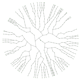
Figure 6: Illustration of the transition in the shape of the pruned tree. On the left, we have represented a tree $\mathbf{t}$ with mean offspring $\nu=1.5$ and $n=15$ generations. On the right, the picture represents the tree $\mathbf{t}^{*}$ obtained by pruning $\mathbf{t}$ with Bernoulli random variables on the leaves of parameters $p_{n}=0.2$. We can observe a change in the pruned tree $\mathbf{t}^{*}$ at generation $k^{*}\simeq 11$; for $k\leqslant k^{*}$, the tree $\mathbf{t}^{*}$ looks like the original tree $\mathbf{t}$, whereas for $k>k^{*}$ mainly thin branches remain.

Recall that if $\mu$ and $\tilde{\mu}$ are two probability measures on a measurable space $(\Omega,\mathcal{A})$, the total variation distance between $\mu$ and $\tilde{\mu}$ is defined by

$$d_{\mathrm{TV}}(\mu,\tilde{\mu}):=\sup_{A\in\mathcal{A}}|\mu(A)-\tilde{\mu}(A)|.$$

An important property of the total variation is that it can be rewritten as $d_{\mathrm{TV}}(\mu,\nu)=\inf_{X\sim\mu,Y\sim\tilde{\mu}}\mathbb{P}(X\neq Y)$, where the infimum is taken over all couplings of $\mu,\tilde{\mu}$, i.e. all (joint) distributions for pairs of random variables $(X,Y)$ whose marginal distributions are $X\sim\mu$ and $Y\sim\tilde{\mu}$.

Proposition 5.7.

There are some constants $c_{4},c_{4}^{\prime}>0$ such that

$$d_{\mathrm{TV}}(\mu_{k}^{*},\mu) \leqslant c_{4}^{\prime}e^{-c_{4}(k^{*}-k)}\qquad\text{ for }k\leqslant k^{*}\,,$$

$$d_{\mathrm{TV}}(\mu_{k}^{*},\mu_{\{1\}}) \leqslant 2\Big{(}\frac{1}{\nu}\Big{)}^{k-k^{*}}\qquad\ \ \text{ for }k\geqslant k^{*}\,,$$

where we denoted by $\mu_{\{1\}}$ the Dirac mass at $1$.

Proof.

Let us start with the case $k\leqslant k^{*}$. Recall the interpretation of $\mu_{k}^{*}$ given by Lemma 4.5: it provides a natural coupling $(X_{k}^{*},X)$ with $X_{k}^{*}\sim\mu_{k}^{*}$ and $X\sim\mu$, where the conditional law of $X_{k}^{*}$ given $X$ is a zero-truncated Binomial $\widehat{\operatorname{Bin}}(X,\delta_{k})$. Then, by the interpretation of the total variation distance in terms of coupling, we obtain

$$d_{\mathrm{TV}}(\mu_{k}^{*},\mu)\leqslant\mathrm{P}(X_{k}^{*}\neq X)=\sum_{d\geqslant 1}\mu(d)\mathrm{P}(B_{k,d}\neq d\mid B_{k,d}>0)\,,$$

with $B_{k,d}\sim\operatorname{Bin}(d,\delta_{k+1})$. As $\gamma_{k+1}\in[0,1]$ and $d\geqslant 1$, we have

$$\mathrm{P}(B_{k,d}=d) =(\delta_{k+1})^{d}=(1-\gamma_{k+1})^{d}\geqslant 1-d\gamma_{k+1}$$

$$\mathrm{P}(B_{k,d}=0) =(1-\delta_{k+1})^{d}=(\gamma_{k+1})^{d}\leqslant\gamma_{k+1}\leqslant\gamma_{k^{*}+1}\quad\text{ for }k\leqslant k^{*}\,,$$

recalling also that $(\gamma_{k})_{k\geqslant 0}$ is non-decreasing for the last inequality (see Lemma 5.3). Since $\gamma_{k^{*}+1}=\bar{\gamma}_{\bar{k}^{*}-1}\leqslant 1-\alpha_{1}$ for some $\alpha_{1}>0$ (see Step 3 of the proof of Proposition 5.4), we therefore have

$$\mathrm{P}(B_{k,d}\neq d\mid B_{k,d}>0)=\dfrac{1-(1-\gamma_{k+1})^{d}}{1-(\gamma_{k+1})^{d}}\leqslant\frac{d}{\alpha_{1}}\,\gamma_{k+1}\,,$$

so $d_{\mathrm{TV}}(\mu_{k}^{*},\mu)\leqslant\frac{1}{\alpha_{1}}\nu\gamma_{k+1}$. This yields the desired upper bound thanks to Proposition 5.4; see also the general bound (5.7).

For the case $k\geqslant k^{*}$, note that for any coupling $(X_{k}^{*},Y)$ such that the marginal distributions are $X_{k}^{*}\sim\mu_{k}^{*}$ and $Y=1$ we have $d_{\mathrm{TV}}(\mu_{k}^{*},\mu_{\{1\}})\leqslant\mathrm{P}(X_{k}^{*}\neq 1)$. Using again Lemma 4.5 that describes the law of $X_{k}^{*}$, we have

$$\mathrm{P}(X_{k}^{*}\neq 1)=\sum_{d\geqslant 2}\mu(d)\mathrm{P}\big{(}B_{k,d}\geqslant 2\mid B_{k,d}>0\big{)},$$

with $B_{k,d}\sim\operatorname{Bin}(d,\delta_{k+1})$. By sub-additivity and Bonferroni’s inequality, we have

$$\mathrm{P}(B_{k,d}\geqslant 2)\leqslant\dfrac{d(d-1)}{2}(\delta_{k+1})^{2},\qquad\mathrm{P}(B_{k,d}\geqslant 1)\geqslant d\delta_{k}-\dfrac{d(d-1)}{2}(\delta_{k+1})^{2}.$$

Thus, we have the bound

$$\mathrm{P}(B_{k,d}\geqslant 2\mid B_{k,d}>0)\leqslant\dfrac{(d-1)(\delta_{k+1})^{2}}{\delta_{k}(2-(d-1)\delta_{k+1})}\,.$$

This gives that $\mathrm{P}(B_{k,d}\geqslant 2\mid B_{k,d}>0)\leqslant\leqslant(d-1)\delta_{k+1}$ for $d\leqslant(\delta_{k+1})^{-1}$, using also that $(\delta_{k})_{k\geqslant 0}$ is non-increasing. Bounding $\mathbb{P}(B_{k,d}\geqslant 2\mid B_{k,d}\geqslant 1)$ by $1$ when $d>(\delta_{k+1})^{-1}$, we get

$$\sum_{d\geqslant 2}\mu(d)\mathrm{P}(B_{k,d}\geqslant 2\mid B_{k,d}>0) \leqslant\sum_{d=2}^{(\delta_{k+1})^{-1}}\mu(d)d\delta_{k+1}+\sum_{d>(\delta_{k+1})^{-1}}\mu(d)$$

$$\leqslant\nu\delta_{k+1}+\mathrm{P}\big{(}X>(\delta_{k+1})^{-1}\big{)}\leqslant 2\nu\delta_{k+1}\,,$$

where we have used Markov’s inequality in the last term. This gives the desired upper bound, using Proposition 5.4. ∎

5.4 Mean of the offspring distribution and size of a generation

In this section we estimate the mean and the variance of the offspring distribution of the pruned tree, and we also observe the phase transition in these quantities. This is not a direct consequence of Proposition 5.7 since the total variation distance does not allow one to control moments. We then estimate the mean size of the generation $k$ of the pruned tree $\mathbf{T}^{*}_{n}$, which will reveal useful in Section 6. Some of the technical estimates of this section are postponed to Appendix A.1.

5.4.1 Mean of $\mu_{k}^{*}$

For $0\leqslant k<n$, we let $X_{k}^{*}$ be a random variable with distribution $\mu_{k}^{*}$ and $\nu_{k}^{*}:=\mathrm{E}[X_{k}^{*}]$ and $(\sigma_{k}^{*})^{2}=\mathrm{Var}(X_{k}^{*})$. We now give several estimates on $\nu_{k}^{*}$, and in particular we observe the phase transition around $k^{*}$. We are also able to estimate the variances $(\sigma_{k}^{*})^{2}$ (which bring other useful information on $\mu_{k}^{*}$), but it is of no particular use for the sequel so we postpone estimates on $(\sigma_{k}^{*})^{2}$ to Appendix A.2.

Remark 5.8.

Recall that in $\mathbf{T}_{n}^{*}$ the offspring distribution of the root is $\tilde{\mu}_{0}^{*}$, see Proposition 4.3. However, when the root is conditioned on having at least one descendant (i.e. $\mathbf{T}_{n}^{*}\neq\emptyset$), which is an event of probability $\delta_{0}$, the offspring distribution of the root is $\mu_{0}^{*}$.

Let us stress that one can easily obtain a formula for $\nu_{k}^{*}$ (we prove it in Appendix A.2, see Lemma A.1):

$$\nu_{k}^{*}:=\mathrm{E}[X_{k}^{*}]=\dfrac{\delta_{k+1}}{\delta_{k}}\nu\,.$$ (5.12)

We can also show that $(\nu_{k}^{*})_{0\leqslant k<n}$ is non-increasing, see Lemma A.2 (also proven in Appendix A.1). We now show that the phase transition observed in Proposition 5.4 translates into the means $(\nu_{k}^{*})_{0\leqslant k<n}$. Recall the definition (5.6) of $k^{*}:=\log_{\nu}(\nu^{n}p_{n})$.

Lemma 5.9.

There are constants $c_{4},c_{5}$ (that depend only on the law $\mu$) such that

$$0\leqslant\nu-\nu_{k}^{*}\leqslant c_{5}e^{-c_{4}(k^{*}-k)} \text{ for }k\leqslant k^{*}\,,$$ (5.13)

$$0\leqslant\nu_{k}^{*}-1\leqslant 1+c_{5}\Big{(}\frac{1}{\nu}\Big{)}^{k-k^{*}} \text{ for }k\geqslant k^{*}\,,$$ (5.14)

where $c_{4}$ is the constant appearing in (5.7).

This lemma shows that $\nu_{k}^{*}$ is very close to $\nu$ if $k^{*}-k\gg 1$ whereas $\nu_{k}^{*}$ is very close to $1$ if $k-k^{*}\gg 1$. Lemma A.3 complements this information by controlling the variance of $\mu_{k}^{*}$, which is close to the variance of $\mu$ if $k^{*}-k\gg 1$ whereas it is close to $0$ if $k-k^{*}\gg 1$. This confirms that the pruned tree roughly grows as a Galton–Watson tree with mean $\nu>1$ for $k\leqslant k^{*}$ (i.e. with an exponential growth rate $\nu$) and then the tree does not grow much more since the mean is roughly $1$ for $k\geqslant k^{*}$. We make this statement precise by controlling the mean size of a generation, see Lemma 5.10 below.

Proof of Lemma 5.9.

Let us start with the case $k\leqslant k^{*}$. First of all, using that the parameters $(\delta_{k})_{0\leqslant k<n}$ are non-increasing (see Lemma 5.3), we get from the expression (5.12) of $\nu_{k}^{*}$ the easy bound $\nu_{k}^{*}\leqslant\nu$. On the other hand, using that $\delta_{k}\leqslant 1$, we get from (5.12) that $\nu_{k}^{*}\geqslant\nu\delta_{k+1}$. Since $\delta_{k+1}=1-\gamma_{k+1}$, applying the bound in Proposition 5.4, we obtain (5.13).

For the case $k\geqslant k^{*}$, $\delta_{k}=\bar{\delta}_{n-k}$ verifies $\bar{\delta}_{k+1}=F(\bar{\delta}_{k})$ with $F(t)=1-G(1-t)$, we have thanks to (5.3)

$$\nu\delta_{k+1}(1-\tilde{C}_{\mu}\delta_{k+1})\leqslant\delta_{k}\leqslant\nu\delta_{k+1}.$$

Therefore, using the expression (5.12) for $\nu_{k}^{*}$, we get that

$$1\leqslant\nu_{k}^{*}=\dfrac{\delta_{k+1}}{\delta_{k}}\nu\leqslant\dfrac{1}{1-\tilde{C}_{\mu}\delta_{k+1}}\leqslant 1+2C_{\mu}\delta_{k+1}\,,$$ (5.15)

for all $k$ such that $\tilde{C}_{\mu}\delta_{k+1}\leqslant\frac{1}{2}$, using that $(1-x)^{-1}\leqslant 1+2x$ for $x\in[0,\frac{1}{2}]$. Hence, using the bound in Proposition 5.4, this yields (5.14) for $k\geqslant k_{2}^{*}:=\min\{k\,,\delta_{k+1}\leqslant 1/(2\tilde{C}_{\mu})\}$. Similarly as in the proof of Step 2 of Proposition 5.4, one easily gets that $k_{2}^{*}\leqslant k^{*}+L_{1}^{\prime}$ for some constant $L_{1}^{\prime}$ that depends only on the law $\mu$; adapting the constant, this yields (5.14). ∎

5.4.2 Size of the generations

Recall that $T_{k}^{*}$ designates the set of vertices in the $k$-th generation of the pruned tree $\mathbf{T}^{*}_{n}$ and $|T_{k}^{*}|$ its size. For ease of notations, let us note $Z_{k}=|T_{k}^{*}|$, for $0\leqslant k\leqslant n$. By Proposition 4.3, we have that when the pruned tree is conditioned to be non-empty, $(Z_{k})_{0\leqslant k\leqslant n}$ is an inhomogeneous branching process with offspring distribution $\mu_{k}^{*}$. We can construct $(Z_{k})_{0\leqslant k\leqslant n}$ as follows: set $Z_{0}=1$ and for $0\leqslant k<n$

$$Z_{k+1}=\sum_{a=1}^{Z_{k}}X_{k,a},$$

where $(X_{k,a})_{a\geqslant 1}$ is a family of i.i.d. random variables with distribution $\mu_{k}^{*}$.

More generally and for future use, we may want to study for any $0\leqslant i\leqslant j\leqslant n$ the size $Z_{i,j}$ of the population generated by an individual of generation $i$ up to generation $j$. The distribution of $Z_{i,j}$ can be constructed as follows: $Z_{i,i}=1$ and iteratively, for $j\in\{i,\ldots,n-1\}$, $Z_{i,j+1}=\sum_{a=1}^{Z_{i,j}}X_{k,a}$. Let us now define, for $0\leqslant i<j\leqslant n$,

$$M_{i,j}^{*}:=\mathrm{E}[Z_{i,j}]=\prod_{k=i}^{j-1}\nu_{k}^{*},$$ (5.16)

where $M_{i,i}=1$ by convention. We can now show how the pruned tree growth stabilizes at generation $k^{*}$; recall the definition (5.6) of $k^{*}:=\log_{\nu}(\nu^{n}p_{n})$.

Lemma 5.10.

There are constants $c_{4}$ (from (5.7)), $c_{6},c_{7}$, that depend only on the law $\mu$, such that

$$\big{(}1-e^{-c_{4}(k^{*}-k)}\big{)}(\nu)^{k} \leqslant M_{0,k}^{*}\leqslant(\nu)^{k} \text{ for }k\leqslant k^{*}\,,$$ (5.17)

$$c_{6}(\nu)^{k^{*}} \leqslant M_{0,k}^{*}\leqslant c_{7}(\nu)^{k^{*}} \text{ for }k\geqslant k^{*}\,.$$ (5.18)

This can be summarized in a slightly weaker form as follows: for all $0\leqslant k\leqslant n$,

$$c_{6}^{\prime}(\nu)^{k\wedge k^{*}}\leqslant M_{0,k}^{*}\leqslant c_{7}(\nu)^{k\wedge k^{*}}\,.$$

This lemma properly shows that $M_{0,k}$ grows as $(\nu)^{k}$ up to $k=k^{*}$ and then almost completely stops growing.

Proof.

Notice that the expression of $\nu_{i}^{*}$ in (5.12) yields the following expression of $M_{0,k}^{*}$: for all $0\leqslant k\leqslant n$,

$$M_{0,k}^{*}=\prod_{i=0}^{k-1}\dfrac{\delta_{i+1}}{\delta_{i}}\nu=\dfrac{\delta_{k}}{\delta_{0}}(\nu)^{k}.$$

For $k\leqslant k^{*}$, as the parameters $(\delta_{k})_{0\leqslant k<n}$ are non-increasing (see Lemma 5.3) and $\delta_{0}\leqslant 1$, we have

$$\delta_{k}(\nu)^{k}\leqslant M_{0,k}^{*}=\dfrac{\delta_{k}}{\delta_{0}}(\nu)^{k}\leqslant(\nu)^{k}.$$

Since $\delta_{k}=1-\gamma_{k}$, applying the bound in Proposition 5.4 (or the general bound (5.7)), we get the desired bound.

For $k\geqslant k^{*}$, the upper bound of $\delta_{k}$ from Proposition 5.4 yields

$$M_{0,k}^{*}\leqslant(\nu)^{k}\dfrac{1}{(\nu)^{k-k^{*}}}\dfrac{1}{\delta_{0}}.$$

Since $\delta_{0}$ is close to $1$ (see e.g. Proposition 5.4), we have the right-hand side of (5.18). For the left-hand side, using $\delta_{0}\leqslant 1$ and Proposition 5.4, we have

$$M_{0,k}^{*}\geqslant(\nu)^{k}\delta_{k}\geqslant c_{1}(\nu)^{k^{*}}\,,$$

which concludes the proof. ∎

To conclude this section, we also give some bounds on $M_{n-k,n}^{*}$, i.e. the growth of generations at the top of the tree. This completes the overall picture of the pruned tree. Recall that $\bar{k}^{*}:=n-k^{*}=\log_{\nu}(\frac{1}{p_{n}})$.

Lemma 5.11.

There are constants $c_{8},c_{9}$, that depend only on the law $\mu$, so that

$$\begin{split}1\leqslant M_{n-k,n}^{*}&\leqslant 1+c_{8}\,\Big{(}\frac{1}{\nu}\Big{)}^{\bar{k}^{*}-k},\qquad\text{for }k\leqslant\bar{k}^{*},\\ (\nu)^{k-\bar{k}^{*}}\leqslant M_{n-k,n}^{*}&\leqslant c_{9}\,(\nu)^{k-\bar{k}^{*}},\qquad\qquad\text{for }k\geqslant\bar{k}^{*},\end{split}$$ (5.19)

which can also be summarized as $\max\{1,(\nu)^{k-\bar{k}^{*}}\}\leqslant M_{n-k,n}^{*}\leqslant 1+c(\nu)^{k-\bar{k}^{*}}$.

Proof.

The proof is similar to the above. First of all, we clearly have $M_{n-k,n}^{*}\geqslant 1$. For the upper bounds, we can use that

$$M_{n-k,n}^{*}=\frac{\delta_{n}}{\delta_{n-k}}(\nu)^{k}=\frac{\bar{\delta}_{0}}{\bar{\delta}_{k}}(\nu)^{k}\leqslant\prod_{i=0}^{k-1}(1-\tilde{C}_{\mu}\bar{\delta}_{i})^{-1}\,,$$

where we have used (5.9) for the last inequality. As $(1-x)^{-1}\leqslant 1+x\leqslant e^{x}$, we get that

$$M_{n-k,n}^{*}\leqslant\exp\Big{(}\tilde{C}_{\mu}\sum_{i=0}^{k-1}\bar{\delta}_{i}\Big{)}\leqslant\exp\Big{(}\frac{\tilde{C}_{\mu}}{\nu-1}p_{n}(\nu)^{k}\Big{)}$$

where we have used that $\bar{\delta}_{i}\leqslant p_{n}(\nu)^{i}$ for all $i\geqslant 0$, see Lemma 5.6. Since by definition of $\bar{k}^{*}$ we have $p_{n}=(\nu)^{-\bar{k}^{*}}$, we obtain $M_{n-k,n}^{*}\leqslant\exp(c(\nu)^{k-\bar{k}^{*}})\leqslant 1+c_{9}(\nu)^{k-\bar{k}^{*}}$ for $k\leqslant\bar{k}^{*}$.

For $k\leqslant\bar{k}^{*}$, we use that $1\geqslant\bar{\delta}_{k}\geqslant\bar{\delta}_{\bar{k}^{*}}\geqslant c_{1}$ (see (5.11)) and the fact that $\bar{\delta}_{0}=p_{n}=(\nu)^{-\bar{k}^{*}}$, to obtain

$$(\nu)^{k-\bar{k}^{*}}\leqslant M_{n-k,n}^{*}=\frac{\bar{\delta}_{0}}{\bar{\delta}_{k}}(\nu)^{k}\leqslant\frac{1}{c_{1}}(\nu)^{k-\bar{k}^{*}}\,.$$

This concludes the proof. ∎

6 Ising model on $\mathbf{T}^{*}_{n}$ with plus boundary external field

6.1 Ising model on trees and non-linear capacity

For the Ising model on a tree $\mathbf{t}$ with plus boundary condition, Pemantle and Peres [27] observed that the magnetization of the root (more precisely the log-likelihood ratio) is comparable to the $L^{3}$-capacity, or $3$-capacity, of the tree, equipped with a specific set of resistances. We state this as Theorem 6.4 below, but let us introduce the necessary notation first.

Non-linear $L^{p}$-capacity.

Let us start by defining the $L^{p}$- or $p$-capacity for a given (finite or infinite) tree $\mathbf{t}=(V,E)$ rooted at a vertex $\rho$; we use analogous notation as in [27]. We let $\partial\mathbf{t}$ be the set of maximal paths oriented away from the root. If the tree is finite, we can identify $\partial\mathbf{t}$ with the set of leaves of $\mathbf{t}$. For infinite trees, we assume that there is no leaf and that all paths in $\partial\mathbf{t}$ are infinite.

The tree $\mathbf{t}$ is equipped with a set of resistances on its edges: to each edge $e=uv$ with $u\rightarrow v$, assign a resistance $R_{u}:=R(e)\in\mathbb{R}_{+}$ and a conductance $C_{u}:=C(e)=R(e)^{-1}$. We say that a function $\theta:V\mapsto\mathbb{R}_{+}$ is a flow on the tree $\mathbf{t}$ if for every $u\in V$ it verifies $\theta(u)=\sum_{u\rightarrow v}\theta(v)$, i.e. if the inflow is equal to the outflow at every vertex of the tree. Additionally, we define the strength $|\theta|$ of a flow $\theta$ as $|\theta|:=\sum_{\rho\rightarrow v}\theta(v)$, that is, the total outflow from the root $\rho$. A flow $\theta$ with $|\theta|=1$ is called a unit flow.

Definition 6.1 ($L^{p}$-capacity).

Let $p>1$ and set $s=p-1$. Then we define the $p$-capacity of the tree $\mathbf{t}$ with resistances $(R_{e})_{e\in V}$ as

$$\operatorname{Cap}_{p}(\mathbf{t}):=\sup_{\theta:\mathcal{V}_{p}(\theta)=1}|\theta|\,,\qquad\text{ with }\quad\mathcal{V}_{p}(\theta):=\sup_{y\in\partial\mathbf{t}}\sum_{e\in y}(\theta(e)R(e))^{s}\,.$$

Remark 6.2.

We stress that when $p=2$, by Thomson’s principle, the $2$-capacity $\operatorname{Cap}_{2}(T)$ reduces to the usual electrical effective conductance between the root $\rho$ and the leaves of the tree; we refer to [21, Ch. 2, 3 & 9] for an extensive introduction on electrical networks on graphs.

Then, Pemantle and Peres [27] establish a recursive expression for the $p$-capacity on a tree. Recall that for a vertex $u\in V$, $\mathbf{t}(u)$ denotes the sub-tree of $\mathbf{t}$ consisting of $u$ (as a root) and all descendants of $u$.

Lemma 6.3 (Lemma 3.1 in [27]).

Let $\mathbf{t}$ be a locally finite tree with root $\rho$. Fix $p>1$ and $s=p-1$. For any vertex $u\in V$, define

$$\phi_{p}(u):=R_{u}\operatorname{Cap}_{p}(\mathbf{t}(u)),$$

where $R_{\rho}=1$ by convention; in particular, $\phi(u)=R_{u}$ if $u$ is a leaf. Then, for any vertex $u\in V$, we have

$$\phi_{p}(u)=\sum_{u\rightarrow v}\dfrac{R_{u}}{R_{v}}\dfrac{\phi_{p}(v)}{(1+\phi_{p}(v)^{s})^{1/s}}\,.$$ (6.1)

Relation to Lyons’ iteration.

Lemma 6.3 is reminiscent of the iteration (2.5) for the log-likelihood ratio, namely $r_{\beta}(u)=\sum_{u\rightarrow v}g_{\beta}(r_{\beta}(v))$. Additionally, [27, Lem. 4.2] observes that the function $g_{\beta}(x)=\log(\frac{e^{2\beta}e^{x}+1}{e^{2\beta}+e^{x}})$ verifies

$$\frac{\tanh(\beta)x}{(1+c_{2}x^{2})^{1/2}}\leqslant g_{\beta}(x)\leqslant\frac{\tanh(\beta)x}{(1+c_{1}x^{2})^{1/2}}\,,$$

for some $c_{1},c_{2}>0$. Therefore, a direct consequence of Theorem 3.2 in [27] and of the recursion (2.5) is the following.

Theorem 6.4 (Theorem 3.2 in [27]).

Let $\mathbf{t}$ be a tree with a set of leaves $\partial\mathbf{t}$. There are constants $\kappa_{1},\kappa_{2}$ such that, for the Ising model on $\mathbf{t}$ with plus boundary condition, the log-likelihood ratio of the root verifies

$$\kappa_{1}\operatorname{Cap}_{3}(\mathbf{t})\leqslant r_{\mathbf{t},\beta}^{+}(\rho)\leqslant\kappa_{2}\operatorname{Cap}_{3}(\mathbf{t})\,.$$

Here $\operatorname{Cap}_{3}(\mathbf{t})$ is the $3$-capacity of the tree $\mathbf{t}$ equipped with resistances $R_{u}:=\tanh(\beta)^{-|u|}$.

This result is used in [27] to obtain a criterion for the magnetization of the Ising Model with plus boundary conditions on an infinite tree $\mathbf{t}$: Theorem 2.2 in [27] shows that the root $\rho$ is magnetized if and only if $\operatorname{Cap}_{3}(\mathbf{t})>0$.

The goal of the rest of the section is therefore to estimate the $3$-capacity of the pruned tree $\mathbf{T}_{n}^{*}$. We will prove the following result, which thanks to Theorem 6.4 will conclude the proof of Theorem 3.3; note that Theorem 6.4 applies with a plus boundary condition, but can be adapted to treat the case of a plus boundary external field, see in particular Remark 1.1.

Proposition 6.5.

Let $\mathbf{T}_{n}$ be a Galton–Watson tree with offspring distribution $\mu$ satisfying Assumption 1, and let $\mathbf{T}^{*}_{n}=\mathrm{Pruned}_{h}(\mathbf{T}_{n})$ be the pruned version of $\mathbf{T}_{n}$ with $(h_{v})_{v\in\partial\mathbf{T}}$ given by i.i.d. Bernoulli random variables with parameter $p_{n}\in(0,1]$, as defined in Section 3.2.

• Upper bound. There is a constant $c>0$ such that

$$\mathbf{E}\otimes\mathbb{E}\big{[}\operatorname{Cap}_{3}(\mathbf{T}^{*}_{n})\big{]}\leqslant c\,\alpha_{n}$$ (6.2)

with

$$\alpha_{n}:=\begin{cases}p_{n}(\tanh(\beta)\nu)^{n}&\quad\text{ if }\tanh(\beta)\nu\neq 1\,,\\ \min\{n^{-1/2},p_{n}\}&\quad\text{ if }\tanh(\beta)\nu=1\,.\end{cases}$$

In particular, if $\tanh(\beta)\nu\leqslant 1$ or if $\lim_{n\to\infty}p_{n}(\tanh(\beta)\nu)^{n}=0$, then $\operatorname{Cap}_{3}(\mathbf{T}^{*}_{n})$ converges to $0$ in $L^{1}$, hence in probability.

• Lower bound. If the offspring distribution $\mu$ admits a finite second moment and if $\liminf_{n\to\infty}p_{n}\nu^{n}=+\infty$, we have that

$$\lim_{\varepsilon\downarrow 0}\limsup_{n\to\infty}\mathbf{P}\otimes\mathbb{P}\big{(}\operatorname{Cap}_{3}(\mathbf{T}^{*}_{n})\leqslant\varepsilon\tilde{\alpha}_{n}\big{)}=0\,,$$ (6.3)

with

$$\tilde{\alpha}_{n}:=\begin{cases}\min\{1,p_{n}(\tanh(\beta)\nu)^{n}\}&\quad\text{ if }\tanh(\beta)\nu\neq 1\,,\\ \min\{n^{-1},p_{n}\}&\quad\text{ if }\tanh(\beta)\nu=1\,.\end{cases}$$

In particular, if $\tanh(\beta)\nu>1$ and $\liminf_{n\to\infty}p_{n}(\tanh(\beta)\nu)^{n}>0$, then $\operatorname{Cap}_{3}(\mathbf{T}^{*}_{n})$ remains asymptotically bounded away from $0$; more precisely, $\{\operatorname{Cap}_{3}(\mathbf{T}^{*}_{n})^{-1}\}_{n\geqslant 0}$ is tight.

Remark 6.6.

In the case where $\tanh(\beta)\nu\neq 1$, then we identify the correct order for $\operatorname{Cap}_{3}(\mathbf{T}^{*}_{n})$, hence for the root magnetization: $\min\{1,p_{n}(\tanh(\beta)\nu)^{n}\}$. In the critical case $\tanh(\beta)\nu=1$, we have identified the correct order for the root magnetization only in the case where $p_{n}\leqslant n^{-1}$, but the upper and lower bound differ otherwise.

Remark 6.7.

For the critical Ising model on the Galton–Watson tree, i.e. when one has $\tanh(\beta)\nu=1$ and $p_{n}\equiv 1$, then Proposition 6.5 and Theorem 6.4 give (also applying Markov’s inequality) that for any $\varepsilon>0$

$$\lim_{\varepsilon\downarrow 0}\liminf_{n\to\infty}\mathbf{P}\Big{(}\frac{\varepsilon}{n}\leqslant r_{n}^{+}(\rho)\leqslant\frac{\varepsilon^{-1}}{\sqrt{n}}\Big{)}=1$$

Roughly speaking, it says that the magnetization of the root $r_{n}^{+}(\rho)$ is bounded from above by $O(1/\sqrt{n})$ and from below by $O(1/n)$. To our knowledge, such bounds do not appear in the literature; our lower bound seems not to be optimal so we believe that the root magnetization is of order $1/\sqrt{n}$, at least when the offspring distribution admits a finite second moment.

Proposition 6.5 amounts to estimating the $3$-capacity of an inhomogeneous branching process. We find this question interesting in its own so we try to study this problem in the most general terms. We will use the structure on the pruned tree only at the end of the proof, to conclude the argument; the estimates in Section 5 turn out crucial for this last step.

6.2 Capacity of an inhomogeneous branching process

Let us consider a tree $T$ of depth $n$ generated by a branching process with inhomogeneous, $n$-dependent, offspring distributions $(\mu_{k}^{(n)})_{0\leqslant k<n}$. Note that the offspring distributions may also depend on $n$, as it is the case for the pruned tree $\mathbf{T}_{n}^{*}$, see Proposition 4.3 and the definition (4.2) of $\mu_{k}^{*}$.

For notational convenience, we will simply write $\mu_{k}:=\mu_{k}^{(n)}$, and we assume that $\mu_{k}(0)=0$ for all $k$. We denote $\nu_{k}$ the mean of $\mu_{k}$ (by convention $\nu_{n}=1$) and for $0\leqslant i<j\leqslant n+1$,

$$M_{i,j}:=\prod_{k=i}^{j-1}\nu_{k}\,,$$ (6.4)

with $M_{i,i}=1$ by convention. Hence, $M_{i,j}$ is the mean size of a population generated by a branching process with offspring distribution $(\mu_{k})_{i\leqslant k<j}$. We then have the following result.

Proposition 6.8.

Let $T$ be a tree of depth $n$ generated by an inhomogeneous branching process with offspring distributions $(\mu_{k}^{(n)})_{0\leqslant k<n}$, and associated resistances $(R_{u})_{u\in T}$ given by $R_{u}=R^{-|u|}$ for some fixed $R>0$. Recalling the definition (6.4) of $M_{i,j}$, we have the following upper bound

$$\mathbf{E}\left[\operatorname{Cap}_{3}(T)\right]\leqslant\bigg{(}\sum_{k=1}^{n}\Big{(}\dfrac{1}{R^{k}M_{0,k}}\Big{)}^{2}\bigg{)}^{-1/2}\,.$$ (6.5)

For the lower bound, define for $0\leqslant k\leqslant n-1$ the quantity $v_{k,n}:=1+\sum\limits_{i=k}^{n-1}\frac{\sigma_{i}^{2}}{M_{k,i}}$, where $\sigma_{i}^{2}$ is the variance of the law $\mu_{i}$. Then we have that for any $\varepsilon>0$,

$$\mathbf{P}\left(\operatorname{Cap}_{3}(T)\leqslant\varepsilon\Big{(}\sum_{k=0}^{n}\dfrac{v_{k,n}}{R^{k}M_{0,k}}\Big{)}^{-1}\right)\leqslant\mathbf{P}\big{(}|T_{n}|\leqslant\varepsilon^{1/3}M_{0,n}\big{)}+\varepsilon^{1/3}\,.$$ (6.6)

6.2.1 Upper bound in Proposition 6.8: proof of (6.5)

For $u\in T$, recall the definition $\phi_{p}(u):=R_{u}\operatorname{Cap}_{p}(T(u))$ in Lemma 6.3. Now, consider the random variable $\Phi_{k}:=\phi_{p}(u)$ for some vertex $u\in T_{k}$ chosen uniformly at random from generation $k$. Then, as the number of offspring of vertices in the same generation are independent, by Lemma 6.3 we get for $0\leqslant k<n$, with $s:=p-1$,

$$\Phi_{k}=R\,\sum_{i=1}^{X_{k}}\dfrac{\Phi_{k+1}^{(i)}}{(1+(\Phi_{k+1}^{(i)})^{s})^{1/s}},$$

where $X_{k}$ is a random variable with distribution $\mu_{k}$ and $(\Phi_{k+1}^{(i)})_{i\geqslant 1}$ are i.i.d. copies of $\Phi_{k+1}$. Note that we also have used that $R_{v}=R^{-|v|}$ here.

Taking the expectation we obtain by the branching property

$$\mathbf{E}[\Phi_{k}]=R\,\nu_{k}\,\mathbf{E}\bigg{[}\dfrac{\Phi_{k+1}}{(1+\Phi_{k+1}^{s})^{1/s}}\bigg{]}\,.$$

As the function $x\mapsto x/(1+x^{s})^{1/s}$ is concave, we can apply Jensen’s inequality to the previous expression: we obtain

$$\mathbf{E}[\Phi_{k}]\leqslant R\,\nu_{k}\,\dfrac{\mathbf{E}[\Phi_{k+1}]}{(1+\mathbf{E}[\Phi_{k+1}]^{s})^{1/s}}=\dfrac{R\,\nu_{k}}{(1+\mathbf{E}[\Phi_{k+1}]^{-s})^{1/s}}.$$ (6.7)

Now, defining $z_{k}:=\mathbf{E}[\Phi_{k}]^{-s}$, we can rewrite (6.7) as $z_{k}\geqslant(R\nu_{k})^{-s}(1+z_{k+1})$. By applying this inequality recursively, we obtain that for all $k\leqslant n$,

$$z_{k}\geqslant\sum_{i=k}^{n}\prod_{j=k}^{i}(R\nu_{j})^{-s}+z_{n}\prod_{j=k}^{n-1}(R\nu_{j})^{-s}\geqslant\sum_{i=k}^{n}(R^{i+1-k}M_{k,i+1})^{-s}\,,$$

where we have used the definition (6.4) $M_{k,i+1}:=\prod_{j=k}^{i}\nu_{k}$ for the last inequality. Since $z_{0}=\mathbf{E}[\Phi_{0}]^{-s}$ and $\Phi_{0}=\operatorname{Cap}_{p}(T)$, we get that

$$\mathbf{E}\left[\operatorname{Cap}_{p}(T)\right]\leqslant\bigg{(}\sum_{i=0}^{n-1}\Big{(}\dfrac{1}{R^{i+1}M_{0,i+1}}\Big{)}^{s}\bigg{)}^{-1/s}\,.$$

This gives a general bound on the $p$-capacity $\operatorname{Cap}_{p}(T)$: with $p=3$, $s=2$, this is the bound (6.5), up to an index change. ∎

6.2.2 Lower bound in Proposition 6.8: proof of (6.6)

Step 1. We start by showing that the $2$-capacity of a tree is a lower bound for its $3$-capacity.

Lemma 6.9.

Let $T$ be a tree of depth $n$ with no leaf excepts the vertices at generation $n$ and equipped with resistances $(R_{v})_{v\in T}$. Then, for any $1<p\leqslant p^{\prime}$ we have $\operatorname{Cap}_{p}(T)\leqslant\operatorname{Cap}_{p^{\prime}}(T)$.

Proof.

Our starting point is Lemma 6.3. Recall that, for a vertex $u$ on the tree $T$ we defined $\phi_{p}(u)=R_{u}\operatorname{Cap}_{p}(T(u))$ and that, for any $p>1$, we have $\operatorname{Cap}_{p}(T(u))=1$ when $u$ is a leaf. Then, Lemma 6.3 shows that for any vertex $u\in T$ that is not a leaf we have

$$\phi_{p}(T(u))=\sum_{u\to v}\frac{R_{u}}{R_{v}}\dfrac{\phi_{p}(T(v))}{(1+\phi_{p}(T(v))^{s})^{1/s}}\,,\quad\phi_{p^{\prime}}(T(u))=\sum_{u\to v}\frac{R_{u}}{R_{v}}\dfrac{\phi_{p^{\prime}}(T(v))}{(1+\phi_{p^{\prime}}(T(v))^{s^{\prime}})^{1/s^{\prime}}}\,,$$

with $s=p-1$, $s^{\prime}=p^{\prime}-1$. To conclude the proof of the lemma, it suffices to show that for any $0<s\leqslant s^{\prime}$ we have $(1+x^{s})^{1/s}\geqslant(1+x^{s^{\prime}})^{1/s^{\prime}}$ for any $x\geqslant 0$ and apply this inequality iteratively. But this simply follows from the fact that for $\alpha\in[0,1]$ and any $a,b\geqslant 0$ we have $(a+b)^{\alpha}\leqslant a^{\alpha}+b^{\alpha}$, so that $(1+x^{s^{\prime}})^{s/s^{\prime}}\leqslant 1+x^{s}$. ∎

Let us define $A_{n}:=\sum\limits_{k=0}^{n}\frac{v_{k,n}}{R^{k}M_{0,k}}$. Using Lemma 6.9, we can bound

$$\mathbf{P}\left(\operatorname{Cap}_{3}(T)\leqslant\varepsilon(A_{n})^{-1}\right)\leqslant\mathbf{P}\left(\operatorname{Cap}_{2}(T)\leqslant\varepsilon(A_{n})^{-1}\right)\,.$$

We can therefore focus on the $2$-capacity $\operatorname{Cap}_{2}(T)$ of the tree; recall that this is the effective conductance between the root $\rho$ and the leaves $\partial T$ (see e.g. [21, Ch. 2] for an overview of the theory of electrical networks on graphs). We then write $\operatorname{Cap}_{2}(T)=\mathcal{C}(\rho\leftrightarrow\partial T)=\mathcal{R}(\rho\leftrightarrow\partial T)^{-1}$, where $\mathcal{R}(\rho\leftrightarrow\partial T)$ is the effective resistance between the root $\rho$ and the leaves $\partial T$. We are now reduced to showing the following inequality

$$\mathbf{P}\left(\mathcal{R}(\rho\leftrightarrow\partial T)\geqslant\varepsilon^{-1}A_{n}\right)\leqslant\mathbf{P}\big{(}W_{0,n}\leqslant\varepsilon^{1/3}\big{)}+\varepsilon^{1/3}\,,$$ (6.8)

where $W_{0,n}=|T_{n}|/M_{0,n}$, see (6.10) below.

Step 2. Our second step is to find an upper bound on the resistance $\mathcal{R}(\rho\leftrightarrow\partial T)$. By Thomson’s principle (see [21, §2.4]), we have

$$\mathcal{R}(\rho\leftrightarrow T_{n})=\inf_{\theta:|\theta|=1}\sum_{u\in T}R_{u}\theta(u)^{2}\,,$$ (6.9)

where $\theta$ is a flow on the tree $T$.

An upper bound is therefore obtained simply by choosing a specific flow $\theta$ on $T$: similarly to what is done in [26, Lem. 2.2] (see also [7, Lem. 3.3]), we use the uniform flow $\hat{\theta}$ on $T$. For a vertex $u\in T_{k}$ in the $k$-th generation, we let

$$\hat{\theta}(u):=\dfrac{|T_{k,n}(u)|}{|T_{n}|},$$

where we note $T_{k,n}(u)$ the set of descendants in generation $n$ of the vertex $u$, i.e. of individuals in generation $n-k$ of the sub-tree $T(u)$. We can easily see that the uniform flow $\hat{\theta}$ is a unitary flow: indeed, we have

$$\hat{\theta}(\rho)=\dfrac{1}{|T_{n}|}\sum_{\rho\to v}|T_{1,n}(v)|=1\,.$$

Therefore, by the Thomson principle (6.9), we have

$$\mathcal{R}(\rho\leftrightarrow T)\leqslant\sum_{v\in V}R_{v}\hat{\theta}(v)^{2}=\frac{1}{|T_{n}|^{2}}\sum_{k=0}^{n}\sum_{u\in T_{k}}R^{-k}|T_{k,n}(u)|^{2}\,.$$

Before we work on this upper bound, let us rewrite it using some notation. For $0\leqslant k\leqslant n$ and $u\in T_{k}$, let us define for $\ell\in\{k,\ldots,n\}$

$$W_{k,\ell}(u)=\dfrac{1}{M_{k,\ell}}|T_{k,\ell}(u)|\,,$$ (6.10)

and notice that $(W_{k,\ell}(u))_{k\leqslant\ell\leqslant n}$ is a martingale (with mean $1$). We also denote $W_{0,k}:=|T_{k}|/M_{0,k}$ the martingale $W_{0,k}(\rho)$. Then, we have

$$\begin{split}\mathcal{R}(\rho\leftrightarrow T)&\leqslant\frac{1}{(W_{0,n})^{2}}\sum_{k=0}^{n}R^{-k}\Big{(}\frac{M_{0,n}}{M_{k,n}}\Big{)}^{2}\sum_{v\in T_{k}}W_{k,n}(v)^{2}\\ &\leqslant\frac{1}{(W_{0,n})^{2}}\sum_{k=0}^{n}\frac{R^{-k}}{M_{0,k}}\frac{1}{M_{0,k}}\sum_{v\in T_{k}}W_{k,n}(v)^{2}\,,\end{split}$$ (6.11)

where we have used that $M_{0,n}=M_{0,k}M_{k,n}$.

Step 3. We are now ready to conclude the proof. Using the above inequality and decomposing according to whether $W_{0,n}$ is small or not, we have

$$\mathbf{P}\Big{(}\mathcal{R}(\rho\leftrightarrow T)\geqslant\varepsilon^{-1} A_{n}\Big{)}\leqslant\mathbf{P}\bigg{(}\sum_{k=0}^{n}\frac{R^{-k}}{M_{0,k}}\frac{1}{M_{0,k}}\sum_{v\in T_{k}}W_{k,n}(v)^{2}\geqslant\varepsilon^{-1}(W_{0,n})^{2}A_{n}\bigg{)}$$

$$\leqslant\mathbf{P}\big{(}W_{0,n}\leqslant\varepsilon^{1/3}\big{)}+\mathbf{P}\bigg{(}\sum_{k=0}^{n}\frac{R^{-k}}{M_{0,k}}\frac{1}{M_{0,k}}\sum_{v\in T_{k}}W_{k,n}(v)^{2}\geqslant\varepsilon^{-1/3}A_{n}\bigg{)}$$

$$\leqslant\mathbf{P}\big{(}W_{0,n}\leqslant\varepsilon^{1/3}\big{)}+\varepsilon^{1/3}A_{n}^{-1}\sum_{k=0}^{n}\frac{R^{-k}}{M_{0,k}}\mathbf{E}\big{[}(W_{k,n})^{2}\big{]}\,,$$

where we have used Markov’s inequality for the last part, together with the fact that $(W_{k,n}(v))_{v\in T_{k}}$ are i.i.d.; here $W_{k,n}$ denotes a random variable with the same distribution. Now, $(|T_{k,\ell}|)_{0\leqslant\ell\leqslant n}$ is an inhomogeneous branching process with offspring distribution $(\mu_{\ell})_{k\leqslant\ell<n}$: it is standard to get that

$$\mathbf{E}\big{[}|T_{k,\ell+1}|^{2}\big{]}=(\nu_{\ell})^{2}\mathbf{E}\big{[}|T_{k,\ell}|^{2}\big{]}+\sigma_{\ell}^{2}\mathbf{E}\big{[}|T_{k,\ell}|\big{]}=(\nu_{\ell})^{2}\mathbf{E}\big{[}|T_{k,\ell}|^{2}\big{]}+\sigma_{\ell}^{2}M_{k,\ell}\,,$$

where $\sigma_{\ell}^{2}$ is the variance of the law $\mu_{\ell}$. Iterating, we get that

$$\mathbf{E}\big{[}|T_{k,n}|^{2}\big{]}=(M_{k,n})^{2}+\sum_{i=k}^{n-1}(M_{i,n})^{2}\sigma_{i}^{2}M_{k,i}\,,\quad\text{ so }\ \mathbf{E}[(W_{k,n})^{2}]=1+\sum_{i=k}^{n-1}\frac{\sigma_{i}^{2}}{M_{k,i}}=:v_{k,n}\,.$$

This concludes the proof of (6.6), recalling the definition of $A_{n}$. ∎

6.3 Conclusion of the proof of Proposition 6.5

We now apply Proposition 6.8 to obtain an upper and a lower bound on $\operatorname{Cap}_{3}(\mathbf{T}^{*}_{n})$, which is the content of Proposition 6.5.

6.3.1 Upper bound on $\operatorname{Cap}_{3}(\mathbf{T}^{*}_{n})$: proof of (6.2)

By Proposition 6.8, we have that

$$\mathbf{E}\otimes\mathbb{E}\big{[}\operatorname{Cap}_{3}(\mathbf{T}_{n}^{*})\big{]}\leqslant\bigg{(}\sum_{k=1}^{n}\Big{(}\dfrac{1}{R^{k}M_{0,k}^{*}}\Big{)}^{2}\bigg{)}^{-1/2}\,,$$

with $R:=\tanh(\beta)<1$ and $M_{i,j}^{*}$ is defined in (5.16). We now use Lemma 5.10 to get that

$$c_{7}^{-1}K_{n}\leqslant\sum_{k=1}^{n}\Big{(}\dfrac{1}{R^{k}M_{0,k}^{*}}\Big{)}^{2}\leqslant c_{6}^{-1}K_{n}\,,\qquad\text{ with }K_{n}:=\sum_{k=1}^{n}R^{-2k}(\nu)^{-2(k\wedge k^{*})}\,.$$

Now, we can easily study $K_{n}$ depending on the value of $R\nu$; note that we only need a lower bound on $K_{n}$ since the above shows that $\mathbf{E}\otimes\mathbb{E}[\operatorname{Cap}_{3}(\mathbf{T}_{n}^{*})]\leqslant cK_{n}^{-1/2}$.

• If $R\nu\neq 1$, then keeping only the term $k=n$ in the sum, we have

$$K_{n}\geqslant(\nu)^{-2k^{*}}R^{-2n}=\Big{(}\frac{1}{p_{n}(R\nu)^{n}}\Big{)}^{2}\,,$$

where we have used that $n-k^{*}=\log_{\nu}(\frac{1}{p_{n}})$. We end up with

$$\mathbf{E}\otimes\mathbb{E}\big{[}\operatorname{Cap}_{3}(\mathbf{T}_{n}^{*})\big{]}\leqslant c\,p_{n}(R\nu)^{n}\,,$$

which gives (6.2) in the case $R\nu\neq 1$. Note that it goes to zero if $\lim_{n\to\infty}p_{n}(R\nu)^{n}=0$.

• If $R\nu=1$, then we have

$$K_{n}\geqslant\sum_{k=1}^{k^{*}}1+\sum_{k=k^{*}+1}^{n}R^{-2(k-k^{*})}\geqslant k^{*}+R^{-2(n-k^{*})}\geqslant\max\{k^{*},p_{n}^{-2}\}\,,$$

where we have used that $R^{n-k^{*}}=1/\nu^{n-k^{*}}$ with $\nu^{n-k^{*}}=\nu^{\bar{k}^{*}}=\frac{1}{p_{n}}$, by the definition (5.6) of $\bar{k}^{*}$. Now, notice that $k^{*}=n-\log_{\nu}(\frac{1}{p_{n}})$ so either $p_{n}\leqslant n^{-1/2}$, or $p_{n}\geqslant n^{-1/2}$ and then $k^{*}\geqslant n/2$. We therefore end up with $K_{n}\geqslant c\max\{n,p_{n}^{-2}\}$, so that

$$\mathbf{E}\otimes\mathbb{E}\big{[}\operatorname{Cap}_{3}(\mathbf{T}_{n}^{*})\big{]}\leqslant c^{\prime}\min\big{\{}n^{-1/2},p_{n}\big{\}}\,.$$

This concludes the proof of (6.2) in the case $R\nu=1$. ∎

6.3.2 Lower bound on $\operatorname{Cap}_{3}(\mathbf{T}^{*}_{n})$: proof of (6.3)

Applying Proposition 6.8, we need to control the two quantities in (6.6). We treat them in the two following lemmas.

Lemma 6.10.

Let $\sigma_{k}^{*}$ be the variance of the law $\mu_{k}^{*}$ and $M_{k,i}=\prod_{j=k}^{i-1}\nu_{j}^{*}$ as defined in (5.16). Then, there exists a constant $C>0$ such that for all $0\leqslant k\leqslant n$

$$v_{k,n}^{*}:=1+\sum_{i=k}^{n-1}\frac{(\sigma_{i}^{*})^{2}}{M_{k,i}^{*}}\leqslant C\,.$$

Lemma 6.11.

Let $W_{0,n}^{*}=\frac{1}{M_{0,n}^{*}}|T_{n}^{*}|$. Then, if $\liminf_{n\to\infty}p_{n}\nu^{n}=+\infty$, we have

$$\lim_{\varepsilon\downarrow 0}\limsup_{n\to\infty}\mathbb{P}\big{(}W_{0,n}\leqslant\varepsilon\big{)}=0\,.$$

Using these two lemmas, we get from Proposition 6.8 that

$$\lim_{\varepsilon\downarrow 0}\limsup_{n\to\infty}\mathbf{P}\otimes\mathbb{P}\bigg{(}\operatorname{Cap}_{3}(\mathbf{T}^{*}_{n})\leqslant\varepsilon\Big{(}\sum_{k=1}^{n}\frac{1}{R^{k}M_{0,k}^{*}}\Big{)}^{-1}\bigg{)}=0\,,$$

Using again Lemma 5.10 to bound $M_{0,k}^{*}$, we get that

$$c\tilde{K}_{n}\leqslant\sum_{k=1}^{n}\frac{1}{R^{k}M_{0,k}^{*}}\leqslant c^{\prime}\tilde{K}_{n}\quad\text{ with }\ \tilde{K}_{n}:=\sum_{k=1}^{k^{*}}(R\nu)^{-k}+(\nu)^{-k^{*}}\sum_{k=k^{*}+1}^{n}R^{-k}\,,$$

so that $\lim_{\varepsilon\downarrow 0}\limsup_{n\to\infty}\mathbf{P}\otimes\mathbb{P}(\operatorname{Cap}_{3}(\mathbf{T}^{*}_{n})\leqslant\varepsilon(\tilde{K}_{n})^{-1})=0$ and we now need to control $\tilde{K}_{n}$ depending on the value of $R\nu$; note that we only need an upper bound.

• If $R\nu\neq 1$, since $R=\tanh(\beta)<1$, we have that

$$\tilde{K}_{n}\leqslant\frac{1}{R\nu-1}\big{(}1-(R\nu)^{-k^{*}}\big{)}+c(\nu)^{-k^{*}}R^{-n}\leqslant c^{\prime}+\frac{c^{\prime\prime}}{(R\nu)^{k^{*}}}+\frac{c}{p_{n}(R\nu)^{n}}\,,$$

where we have used that $(\nu)^{n-k^{*}}=1/p_{n}$ by definition (5.6) of $k^{*}$. In the case $R\nu<1$ (where we already know that $\operatorname{Cap}_{3}(\mathbf{T}^{*}_{n})$ goes to $0$ in probability) we get that $\tilde{K}_{n}\leqslant\frac{c}{p_{n}(R\nu)^{n}}$; note that this upper bound diverges. In the case $R\nu>1$ the upper bound is a constant times $\max\{1,\frac{1}{p_{n}(R\nu)^{n}}\}$. This concludes the proof of (6.3) in the case $R\nu\neq 1$.

Note that in the case where $R\nu>1$ and $\liminf_{n\to\infty}p_{n}(R\nu)^{n}>0$, then $\limsup_{n\to\infty}(\tilde{K}_{n})^{-1}<+\infty$, so it proves in particular that $\lim_{\varepsilon\downarrow 0}\limsup_{n\to\infty}\mathbf{P}\otimes\mathbb{P}\big{(}\operatorname{Cap}_{3}(\mathbf{T}^{*}_{n})\leqslant\varepsilon\big{)}=0$.

• If $R\nu=1$, then similarly to the above, we have

$$\tilde{K}_{n}\leqslant k^{*}+c(\nu)^{-k^{*}}R^{-n}\leqslant c^{\prime}\max\{k^{*},(\nu)^{n-k^{*}}\}=c^{\prime}\max\big{\{}k^{*},p_{n}^{-1}\big{\}}$$

recalling that $(\nu)^{n-k^{*}}=1/p_{n}$. This concludes the proof of (6.3) in the case $R\nu=1$. ∎

6.3.3 Last technical lemmas: proof of Lemmas 6.10 and 6.11

Proof of Lemma 6.10.

We start with the case where $k\geqslant k^{*}$. Then, splitting the sum in the definition of $v_{k,n}^{*}$ (see 6.8) according to whether $i\leqslant k^{*}$ or $i\geqslant k^{*}$, we obtain

$$v_{k,n}^{*}=1+\sum_{i=k}^{k^{*}}\frac{(\sigma_{i}^{*})^{2}}{M_{k,i}^{*}}+\sum_{i=k^{*}+1}^{n-1}\frac{(\sigma_{i}^{*})^{2}}{M_{k,i}^{*}}\leqslant 1+c\sum_{i=k}^{k^{*}}\nu^{-(i-k)}+\sum_{i=k^{*}+1}^{n-1}(\sigma_{i}^{*})^{2}\,,$$

where we have used that $(\sigma_{i}^{*})^{2}\leqslant m_{2}$, see Remark A.4, that $M_{k,i}^{*}=\frac{M_{0,i}^{*}}{M_{0,k}^{*}}\geqslant c(\nu)^{i-k}$ for $k\leqslant i\leqslant k^{*}$ thanks to Lemma 5.10, and finally that $M_{k,i}^{*}\geqslant 1$ in the case $i\geqslant k^{*}$. The first sum is finite since $\nu>1$, and the second sum is also finite, using that $(\sigma_{i}^{*})^{2}\leqslant c\nu^{-(i-k^{*})}$ for $i>k^{*}$, see Lemma A.3.

In the case where $k<k^{*}$, then we have similarly

$$v_{k,n}^{*}=1+\sum_{i=k}^{n-1}\frac{(\sigma_{i}^{*})^{2}}{M_{k,i}^{*}}\leqslant 1+\sum_{i=k}^{n-1}(\sigma_{i}^{*})^{2}\,,$$

that last sum being also bounded by a universal constant. ∎

Proof of Lemma 6.11.

First of all, let us observe that in the general case of a branching process with inhomogeneous, $n$-dependent, offspring distributions $(\mu_{k}^{(n)})_{1\leqslant k\leqslant n}$, one cannot use a martingale convergence as one would for a homogeneous branching process. For the pruned tree, we now give some ad-hoc proof, which uses the structure of the tree. For completeness, we give in Appendix A.3 and alternative line of proof that one should follow in the general case.

In the case of the pruned tree $\mathbf{T}_{n}^{*}$, we use the fact that the distribution of $|T_{n}^{*}|$ is explicit: conditionally on $|T_{n}|$, it is a binomial $\operatorname{Bin}(|T_{n}|,p_{n})$. In particular,

$$M_{0,n}^{*}:=\mathbf{E}\big{[}|T_{n}^{*}|\mid|T_{n}^{*}|>1\big{]}=\delta_{0}^{-1}\mathbf{E}\big{[}|T_{n}^{*}|\big{]}=\delta_{0}^{-1}p_{n}\nu^{n}\,,$$

with $\delta_{0}$ close to $1$. We therefore get that

$$\begin{split}\mathbf{P}\big{(}|T_{n}^{*}|\leqslant\varepsilon M_{0,n}\big{)}&\leqslant\mathbf{P}\big{(}|T_{n}|\leqslant 2\varepsilon\nu^{n}\big{)}+\mathbf{P}\big{(}|T_{n}|\geqslant 2\varepsilon\nu^{n},\operatorname{Bin}(|T_{n}|,p_{n})\leqslant\varepsilon\delta_{0}^{-1}p_{n}\nu^{n}\big{)}\\ &\leqslant\mathbf{P}\big{(}|T_{n}|\leqslant 2\varepsilon\nu^{n}\big{)}+\mathbf{P}\big{(}\operatorname{Bin}(2\varepsilon\nu^{n},p_{n})\leqslant\varepsilon\delta_{0}^{-1}p_{n}\nu^{n}\big{)}\,.\end{split}$$

The second probability clearly goes to $0$, as long as $\liminf_{n\to\infty}p_{n}\nu^{n}=+\infty$ (using also that $\delta_{0}$ goes to $1$). For the first probability, we use that $\mathbf{T}$ is a homogeneous branching process: we have that $(\frac{1}{\nu^{n}}|T_{n}|)_{n\geqslant 0}$ is a martingale that converges almost surely to a positive random variable $\mathcal{W}$ (recall we assumed that $\mu(0)=0$). Hence, we get that

$$\limsup_{n\to\infty}\mathbf{P}\big{(}|T_{n}^{*}|\leqslant\varepsilon M_{0,n}\big{)}\leqslant\mathbf{P}(\mathcal{W}\leqslant 2\varepsilon)\,,$$

which goes to $0$ as $\varepsilon\downarrow 0$ and concludes the proof. ∎

Appendix A Some technical proofs and comments

A.1 About recursions: proofs of Lemmas 5.1 and 5.2

Proof of Lemma 5.1.

Recall that $G$ is the generating function of a random variable $X\in\mathbb{N}$ with mean $m_{1}$ and second moment $m_{2}$.

For (5.1), by the Taylor-Lagrange theorem, for all $s\in[0,1]$ there exists $x_{1}\in[s,1]$ such that:

$$G(s)=G(1)+G^{\prime}(1)(s-1)+\dfrac{G^{\prime\prime}(x_{1})}{2}(s-1)^{2}\,.$$ (A.1)

By convexity of the function $G$, we have that $0\leqslant G^{\prime\prime}(x_{1})\leqslant G^{\prime\prime}(1)=m_{2}-m_{1}$. Since $G(1)=1$, $G^{\prime}(1)=m_{1}$, we therefore obtain from (A.1) that for all $s\in[0,1]$

$$1+m_{1}(s-1)\leqslant G(s)\leqslant 1+m_{1}(s-1)+\frac{1}{2}(m_{2}-m_{1})(s-1)^{2}\,,$$

which is the desired bound.

The bounds of (5.2) are easily deduced from the definition $G(s)=\sum_{i\geqslant 1}\mu(i)s^{i}$, using that $s^{i}\leqslant s^{d_{0}+1}$ for $i\geqslant d_{0}+1$ and $\sum_{i\geqslant d_{0}+1}\mu(i)\leqslant 1$ for the upper bound. ∎

Proof of Lemma 5.2.

Thanks to the bounds (5.2), we have for any $j\geqslant 1$

$$\mu(d_{0})\;(u_{j-1})^{d_{0}}\leqslant u_{j}=G(u_{j-1})\leqslant\mu(d_{0})\;(u_{j-1})^{d_{0}}+(u_{j-1})^{d_{0}+1}.$$

Thus, by iteration, we obtain for $j\geqslant 1$,

$$\prod_{i=0}^{j-1}\mu(d_{0})^{d_{0}^{i}}\times(u_{0})^{d_{0}^{j}}\leqslant u_{j}\leqslant\prod_{i=0}^{j-1}\mu(d_{0})^{d_{0}^{i}}\times(u_{0})^{d_{0}^{j-1}}\times\prod_{i=0}^{j-1}\left(1+\dfrac{u_{i}}{\mu(d_{0})}\right)^{d_{0}^{j-1-i}}.$$ (A.2)

(i) In the case $d_{0}=1$, the lower bound is directly given by (A.2). For the upper bound, we only need to control $\prod_{i=0}^{j-1}(1+\frac{1}{\mu(1)}u_{i})$. We use that, $G$ being convex, $G(s)\leqslant p_{\alpha}s$ for all $s\in[0,1-\alpha]$, with $p_{\alpha}=\frac{G(1-\alpha)}{1-\alpha}<1$: we easily deduce by iteration that $u_{i}\leqslant(p_{\alpha})^{i}u_{0}$ for all $i\geqslant 0$. This leads to the following:

$$\prod_{i=0}^{j-1}\Big{(}1+\dfrac{u_{i}}{\mu(1)}\Big{)}\leqslant\exp\Big{(}\dfrac{1}{\mu(1)}\sum_{i=0}^{j-1}u_{i}\Big{)}\leqslant\exp\Big{(}\dfrac{u_{0}}{\mu(1)}\dfrac{1}{1-p_{\alpha}}\Big{)}\leqslant C_{\alpha},$$

with $C_{\alpha}:=e^{\frac{1-\alpha}{\mu(1)(1-p_{\alpha})}}$, which proves (5.4).

(ii) In the case $d_{0}\geqslant 2$, the lower bound is also immediate from (A.2), since $\sum_{i=0}^{j-1}d_{0}^{i}=\frac{d_{0}^{j}-1}{d_{0}-1}$. For the upper bound, let us start by noting that if $\mu(d_{0})=1$, then we have the exact formula $u_{j}=(u_{0})^{d_{0}^{j-1}}$, with $u_{0}\leqslant 1-\alpha$. If $\mu(d_{0})<1$, then there is some $v_{0}\in(0,1)$ such that $G(s)\leqslant s^{d_{0}}$ for all $s\leqslant v_{0}$. Since there is some $j_{\alpha}$ such that $u_{j}\leqslant v_{0}$ for all $j\geqslant j_{\alpha}$, we get as above that for $j\geqslant j_{\alpha}$

$$u_{j}\leqslant(u_{j_{\alpha}})^{d_{0}^{j-j_{\alpha}}}\leqslant\exp\big{(}-(d_{0}^{-j_{\alpha}}\log v_{0})d_{0}^{j}\big{)}\,.$$

Adjusting the constant to deal with the terms $j<j_{\alpha}$, this gives the desired bound. ∎

A.2 Complementary estimates on the offspring distributions $\mu_{k}^{*}$

For $0\leqslant k<n$, let $X_{k}^{*}$ be a random variable with distribution $\mu_{k}^{*}$ (the offspring distribution of the pruned tree) and let $\nu_{k}^{*}$ be its mean and $(\sigma_{k}^{*})^{2}$ its variance.

Recall also Lemma 4.5 which says that $X_{k}^{*}\sim\widehat{\operatorname{Bin}}(X,\delta_{k+1})$, where $\widehat{\operatorname{Bin}}$ denotes a zero-truncated binomial, i.e. a binomial conditioned on being strictly positive, see Definition 4.4, and $X$ is a random variable with law $\mu$. For later reference, if $\hat{B}\sim\widehat{\operatorname{Bin}}(n,p)$, its mean and variance are given by

$$\mathrm{E}\big{[}\hat{B}\big{]}=\dfrac{np}{1-(1-p)^{n}},\qquad\operatorname{Var}(\hat{B})=\dfrac{np}{(1-(1-p)^{n})^{2}}\big{(}1-p-(1-p+np)(1-p)^{n}\big{)}.$$ (A.3)

Recall that $\nu$, $m_{2}$ denote the first and second moment of the offspring distribution $\mu$.

Lemma A.1.

Let $X_{k}^{*}$ be a random variable with distribution $\mu_{k}^{*}$. then

$$\nu_{k}^{*} :=\mathrm{E}[X_{k}^{*}]=\dfrac{\delta_{k+1}}{\delta_{k}}\nu,$$

$$(\sigma_{k}^{*})^{2} :=\operatorname{Var}(X_{k}^{*})=\nu_{k}^{*}\Big{(}1+\delta_{k+1}\Big{(}\frac{m_{2}}{\nu}-1\Big{)}-\nu_{k}^{*}\Big{)}\,.$$

Proof of Lemma A.1.

Letting $B_{k}\sim\mathrm{Bin}(X,\delta_{k+1})$, we have thanks to Lemma 4.5 that

$$\nu_{k}^{*}=\sum_{z\geqslant 1}z\mathrm{P}(X_{k}^{*}=z)=\sum_{z\geqslant 1}z\dfrac{\mathrm{P}(B_{k}=z)}{\mathrm{P}(B_{k}>0)}=\dfrac{1}{\delta_{k}}\sum_{z\geqslant 1}z\mathrm{P}(B_{k}=z),$$

where we have used that $\mathrm{P}(B_{k}=0)=\gamma_{k}$ so $\mathrm{P}(B_{k}>0)=\delta_{k}$, see the proof of Lemma 4.5. Working with the definition of $B_{k}$, we easily see that

$$\sum_{z\geqslant 1}z\mathrm{P}(B_{k}=z)=\sum_{d\geqslant 1}\mu(d)\mathrm{E}\big{[}\operatorname{Bin}(d,\delta_{k+1})\big{]}=\delta_{k+1}\sum_{d\geqslant 0}\mu(d)d=\delta_{k+1}\nu\,.$$

For the expression of the variance, let us compute the second moment of $X_{k}^{*}$: for $0\leqslant k<n$, similarly as above we have

$$\begin{split}\mathrm{E}\big{[}(X_{k}^{*})^{2}\big{]}=\dfrac{1}{\delta_{k}}\sum_{z\geqslant 1}z^{2}\mathrm{P}(B_{k}=z)&=\dfrac{1}{\delta_{k}}\sum_{d\geqslant 0}\mu(d)\mathrm{E}\big{[}\operatorname{Bin}(d,\delta_{k+1})^{2}\big{]}\\ &=\dfrac{1}{\delta_{k}}\big{(}\delta_{k+1}\gamma_{k+1}\nu+\delta_{k+1}^{2}m_{2}\big{)}.\end{split}$$

Thus, by computing $\mathrm{E}[(X_{k}^{*})^{2}]-\mathrm{E}[X_{k}^{*}]^{2}$, we get the following expression for the variance:

$$(\sigma_{k}^{*})^{2}=\dfrac{\delta_{k+1}}{\delta_{k}}\left(\gamma_{k+1}\nu+\delta_{k+1}m_{2}-\dfrac{\delta_{k+1}}{\delta_{k}}(\nu)^{2}\right)\,,$$

which gives the correct expression, using the formula for $\nu_{k}^{*}$. ∎

We now give some property of the means $(\nu_{k}^{*})_{0\leqslant k<n}$.

Lemma A.2.

The sequence of means $(\nu_{k}^{*})_{0\leqslant k<n}$ is non-increasing.

Proof.

We start by writing $\nu_{k}^{*}$ only in terms of the random variable $X$ with distribution $\mu$ and of the parameter $\gamma_{k+1}$. Note that, since conditionally on $X$ the random variable $B_{k}$ is a zero-truncated binomial $\widehat{\operatorname{Bin}}(X,1-\gamma_{k+1})$, we have

$$\mathrm{E}[X_{k}^{*}\mid X]=\dfrac{X(1-\gamma_{k+1})}{1-(\gamma_{k+1})^{X}}.$$

Thus, $\nu_{k}^{*}=\mathrm{E}[f(\gamma_{k+1},X)]$ for $f(x,y):=\dfrac{y(1-x)}{1-x^{y}}$. As $X\geqslant 1$ and $\gamma_{k+1}\in[0,1]$ is non-decreasing, it is enough to prove that $x\mapsto f(x,y)$ is non-increasing on $[0,1]$, for any $y\geqslant 1$.

Fix $y\geqslant 1$ and let $f_{y}(x):=f(x,y)$, $g_{y}(x):=x^{y}-1+yx^{y-1}(1-x)$ for $x\in[0,1]$. Thus, we can write

$$f^{\prime}_{y}(x)=\dfrac{y}{(1-x^{y})^{2}}g_{y}(x).$$

We can easily see that, for $y\geqslant 1$ and $x\in[0,1]$, we have $g_{y}(x)\leqslant 0$, as $g_{y}(0)=-1$, $g_{y}(1)=0$ and $x\mapsto g_{y}(x)$ is non-decreasing. Therefore, $f^{\prime}_{y}(x)\leqslant 0$ for $x\in[0,1]$, which concludes the proof. ∎

Let us now study the variances $((\sigma_{k}^{*})^{2})_{0\leqslant k<n}$ and prove a statement analogous to Lemma 5.9; in particular we also observe the phase transition from Proposition 5.4 in terms of the variances. Recall the definition (5.6) of $k^{*}:=\log_{\nu}(\nu^{n}p_{n})$.

Lemma A.3.

There are constants $c,c^{\prime}$ (that depend only on the law $\mu$) such that:

$$(\sigma_{k}^{*})^{2} \leqslant c\,\Big{(}\frac{1}{\nu}\Big{)}^{k-k^{*}} \text{ for }k\geqslant k^{*},$$ (A.4)

$$|(\sigma_{k}^{*})^{2}-\sigma^{2}| \leqslant c^{\prime}e^{-c_{4}(k^{*}-k)} \text{ for }k\leqslant k^{*}\,.$$ (A.5)

Remark A.4.

Note that we have no monotonicity for the sequence $(\sigma_{k}^{*})_{0\leqslant k\leqslant n-1}$, nor the upper bound $(\sigma_{k}^{*})^{2}\leqslant\sigma^{2}$ in general. Indeed, choosing $\mu(d_{0})=1$ for some $d_{0}\geqslant 2$, then $\sigma^{2}=0$ but $(\sigma_{k}^{*})^{2}>0$, since then $\mu_{k}^{*}$ is a zero-truncated binomial $\widehat{\operatorname{Bin}}(d,\bar{\delta}_{k+1})$. On the other hand, we have a general (easy) bound: $(\sigma_{k}^{*})^{2}\leqslant\mathrm{E}[\widehat{\operatorname{Bin}}(X,\delta_{k+1})^{2}]\leqslant\mathrm{E}[X^{2}]=:m_{2}$.

Proof.

Recall from Lemma A.1 the formula: $(\sigma_{k}^{*})^{2}=\nu_{k}^{*}\big{(}1+\delta_{k+1}(\frac{m_{2}}{\nu}-1)-\nu_{k}^{*}\big{)}$.

For $k\geqslant k^{*}$, using Lemma 5.9, we get that $\nu_{k}^{*}\leqslant m_{1}$ and $1-\nu_{k}^{*}\leqslant 0$, so

$$(\sigma_{k}^{*})^{2}\leqslant\delta_{k+1}(m_{2}-\nu)\,,$$

and we directly get the upper bound (A.4) thanks to Proposition 5.4.

For $k\leqslant k^{*}$, using that $\delta_{k+1}=1-\gamma_{k+1}$ and setting $\varepsilon_{k}:=\nu-\nu_{k}^{*}\geqslant 0$, we have (bounding also $\nu_{k}^{*}\leqslant\nu$),

$$(\sigma_{k}^{*})^{2}\leqslant\nu\Big{(}1-\nu+\varepsilon_{k}+\frac{m_{2}}{\nu}-1-\gamma_{k+1}\Big{(}\frac{m_{2}}{\nu}-1\Big{)}\Big{)}\leqslant\sigma^{2}+\varepsilon_{k}\nu\,,$$

where we have used that $\frac{m_{2}}{\nu}-1\geqslant 0$. Using Lemma 5.9, we get the desired upper bound. For the lower bound, we write similarly

$$(\sigma_{k}^{*})^{2}\geqslant(\nu-\varepsilon_{k})\Big{(}1-\nu+\frac{m_{2}}{\nu}-1-\gamma_{k+1}\Big{(}\frac{m_{2}}{\nu}-1\Big{)}\Big{)}\geqslant\sigma^{2}-\frac{\sigma^{2}}{\nu}\varepsilon_{k}-\gamma_{k+1}(m_{2}-\nu)\,.$$

Using Lemma 5.9 and Proposition 5.4, this concludes the proof. ∎

A.3 About general inhomogeneous, $n$-dependent, branching processes: alternative proof of Lemma 6.11

In this section, we give an alternative proof of Lemma 6.11, following a different scheme of proof that remains valid for general inhomogeneous, $n$-dependent, branching processes $T$, with offspring distribution $(\mu_{k}^{(n)})_{0\leqslant k<n}$; note that what makes the result non-trivial is precisely the $n$-dependence since one cannot use almost sure martingale convergence results. We denote $\nu_{k},\sigma_{k}^{2}$ the mean and variance of $\mu_{k}=\mu_{k}^{(n)}$.

We define $W_{0,n}:=\frac{1}{M_{0,n}}|T_{n}|$ as in Section 6.2 and we want to control $\mathbf{P}(W_{0,n}\leqslant\varepsilon)$. Equivalently to Lemma 6.11, we want to prove the following:

$$\lim_{\lambda\to\infty}\limsup_{n\to\infty}\mathbf{E}\big{[}e^{-\lambda W_{0,n}}\big{]}=0\,.$$ (A.6)

We let $G_{k}=G_{k}^{(n)}$ be the generating function of $\mu_{k}$ (recall we assumed $\mu_{k}(0)=0$),

$$G_{k}(s):=\sum_{d=1}^{\infty}\mu_{k}(d)s^{d}\qquad s\in[0,1]$$

and we note that $G_{T_{n}}=G_{0}\circ G_{1}\circ\cdots\circ G_{n-1}$ is the generating function of $T_{n}$. Hence, we can rewrite $\mathbf{E}[e^{-\lambda W_{0,n}}]=G_{T_{n}}(e^{-\lambda/M_{0,n}})$. Since, for any fixed $\lambda>0$ and $n$ large enough, we have $e^{-\lambda/M_{0,n}}\leqslant 1-\frac{\lambda}{2M_{0,n}}$, we get that (A.6), hence Lemma 6.11 is equivalent to having

$$\lim_{\lambda\to\infty}\limsup_{n\to\infty}G_{T_{n}}\Big{(}1-\frac{\lambda}{M_{0,n}}\Big{)}=0\,.$$ (A.7)

Let us describe the general strategy to prove (A.7). For $s\in(0,1)$, define the sequence $(\bar{\Gamma}_{k}(s))_{0\leqslant k\leqslant n}$ as

$$\begin{split}\bar{\Gamma}_{0}(s)&:=\bar{\Gamma}_{0}=s\\ \bar{\Gamma}_{k}(s)&:=\bar{\Gamma}_{k}=G_{n-k}\circ\cdots\circ G_{n-1}(s)=G_{n-k}(\bar{\Gamma}_{k-1})\,.\end{split}$$

Note that we keep the notation $\bar{\Gamma}_{k}$ (instead of $\Gamma_{k}$) in analogy with Section 5, since we index our quantities in terms of the distance to the leaves.

The general strategy of proof can then be decomposed into the following steps:

• Find $\bar{\kappa}=\bar{\kappa}(\lambda,n)$ such that for $s:=1-\frac{\lambda}{M_{0,n}}$ we have $\bar{\Gamma}_{\bar{\kappa}}(s)\leqslant 1-\eta$, for some universal constant $\eta>0$.

  Informally, $\bar{\kappa}$ is the number of steps needed for $\bar{\Gamma}_{k}(s)$ to start getting away from $1$.

• Show that $n-\bar{\kappa}\geqslant\kappa_{0}(\lambda)$ uniformly in $n$, with $\lim_{n\to\infty}\kappa_{0}(\lambda)=+\infty$.

  Informally, this tells that after $\bar{\kappa}$ iterations there are still many iterations remaining.

• Show that for any $\eta>0$ and any $\varepsilon>0$, there exists some universal $k_{\eta,\varepsilon}>0$ (i.e. that does not depend on $n$) such that $G_{0}\circ\cdots\circ G_{k}(1-\eta)\leqslant\varepsilon$ for $k\geqslant k_{\eta,\varepsilon}$.

  Informally, this tells that if one has reached $\bar{\Gamma}_{k}\leqslant 1-\eta$ and that a large number of iterations remains, then $\bar{\Gamma}_{n}:=G_{T_{n}}(1-\frac{\lambda}{M_{0,n}})$ is small.

These three steps indeed allow us to prove (A.7): applying Step 1, we have by monotonicity of the generating functions,

$$G_{T_{n}}\Big{(}1-\frac{\lambda}{M_{0,n}}\Big{)}\leqslant G_{0}\circ\cdots\circ G_{n-\bar{\kappa}^{*}}(1-\eta)\,.$$

Then, applying Step 2 in the second inequality (together with the fact that $G_{i}(s)\leqslant s$) for any $s\in[0,1]$, we get that

$$G_{T_{n}}\Big{(}1-\frac{\lambda}{M_{0,n}}\Big{)}\leqslant G_{0}\circ\cdots\circ G_{\kappa_{0}(\lambda)}(1-\eta)$$

Step 3 above, together with the fact that $\kappa_{0}(\lambda)\to\infty$ as $\lambda\to\infty$ concludes the proof.

Remark A.5.

More generally, one could simply define some $\bar{\kappa}=\bar{\kappa}(n,\lambda)$, show some upper bound $\bar{\Gamma}_{\bar{\kappa}}(s)\leqslant 1-\bar{\eta}$ with $\bar{\eta}:=\bar{\eta}(n,\lambda)$, and then prove that $G_{0}\circ\cdots G_{n-\bar{\kappa}}(1-\eta)\to 0$. One should think of the three steps described above as the general scheme one should follow to prove (A.7). We refer to (A.15) for a general sufficient condition to get (A.7).

We now perform these three steps in a general framework: for the first two steps, we give an explicit candidate for $\bar{\kappa}$, see (A.10), and a bound for $\bar{\Gamma}_{\bar{\kappa}}$ in terms of $\bar{\kappa}$, see (A.11). We apply these to the inhomogeneous branching process $\mathbf{T}^{*}_{n}$, where all quantities are explicit.

Step 1. For $s\in(0,1)$, we define

$$\bar{\kappa}:=\bar{\kappa}(n,s):=\max\Big{\{}0\leqslant k\leqslant n\,,\sum_{i=n-k+1}^{n}\frac{\tilde{C}_{i-1}}{M_{0,i}}<\frac{1}{2M_{0,n}(1-s)}\Big{\}}\,,$$

where $\tilde{C}_{j}:=\frac{1}{2}(\frac{\sigma_{j}^{2}}{\nu_{j}}+\nu_{j}-1)$. We then have the following result, which helps us deal with the first step of the proof (its proof is analogous to that of Proposition 5.4).

Lemma A.6.

For $s\in(0,1)$, there is a constant $c_{9}$ that depend only on $\mu$, such that

$$c_{9}M_{n-k,n}(1-s)\leqslant 1-\bar{\Gamma}_{k}(s)\leqslant M_{n-k,n}(1-s)\quad\text{for all }k\leqslant\bar{\kappa}\,.$$ (A.8)

The upper bound holds for any $0\leqslant k\leqslant n$.

Proof.

Let us define $\bar{\Delta}_{k}:=1-\bar{\Gamma}_{k}$, which satisfies the recursion: $\bar{\Delta}_{0}=1-s$, $\bar{\Delta}_{k}=F_{n-k}(\bar{\Delta}_{k-1})$, with $F_{j}(s):=1-G_{j}(1-s)$. Note that as in Lemma 5.1 or (5.3), we have some general bounds for the generating functions $(G_{k})_{0\leqslant k<n}$ or $(F_{k})_{0\leqslant k<n}$, in terms of their first and second moment: for all $0\leqslant k<n$ and for $t\in[0,1]$, we have

$$\nu_{j}t(1-\tilde{C}_{j}t)\leqslant F_{j}(t)\leqslant\nu_{j}t\,,$$ (A.9)

where $\tilde{C}_{j}:=\frac{1}{2\nu_{j}}G_{j}^{\prime\prime}(1)=\frac{1}{2}(\frac{\sigma_{j}^{2}}{\nu_{j}}+\nu_{j}-1)$. Now, the upper bound in (A.8) is a direct recursive application of the right-hand side bound in (A.9).

For the lower bound, we use the following result, which is analogous to Lemma 5.6; we omit its proof as it is very similar. Let $s\in(0,1]$ and set $\bar{\kappa}_{1}(s):=\max\{1\leqslant j\leqslant n\,:\,\sum_{i=0}^{j-1}\tilde{C}_{n-i-1}\bar{\Delta}_{i}(s)<1/2\}$. Then, for all $k\leqslant\bar{\kappa}_{1}$, we have

$$\dfrac{1}{2}M_{n-k,n}(1-s)\leqslant\bar{\Delta}_{k}(s)\leqslant M_{n-k,n}(1-s)\,.$$

Now, notice that by the upper bound on $\bar{\Delta}_{i}(s)$, we have

$$\sum_{i=0}^{j-1}\tilde{C}_{n-i-1}\bar{\Delta}_{i}(s)\leqslant\sum_{i=0}^{j-1}\tilde{C}_{n-i-1}M_{n-i,n}(1-s)=(1-s)M_{0,n}\sum_{i=0}^{j-1}\frac{\tilde{C}_{n-i-1}}{M_{0,n-i}}\,.$$

Hence, $\bar{\kappa}_{1}\geqslant\max\{1\leqslant j\leqslant n\,:\,\sum_{i=0}^{j-1}\frac{\tilde{C}_{n-i-1}}{M_{0,n-i}}\geqslant(2M_{0,n}(1-s))^{-1}\}=:\bar{\kappa}$, which concludes the proof. ∎

Step 2. In the case where $s=1-\frac{\lambda}{M_{0,n}}$, i.e. $M_{0,n}(1-s)=\lambda$, then $\bar{\kappa}$ reduces to

$$\bar{\kappa}:=\bar{\kappa}(n,\lambda):=\max\Big{\{}0\leqslant k\leqslant n\,,\sum_{i=n-k}^{n}\frac{\tilde{C}_{i-1}}{M_{0,i}}<\frac{1}{2\lambda}\Big{\}}\,,$$ (A.10)

and (A.8) in Proposition A.6 gives that for $k=\bar{\kappa}$,

$$\bar{\Gamma}_{\bar{\kappa}}(s)\leqslant 1-M_{n-\bar{\kappa},n}(1-s)=1-\frac{\lambda}{M_{0,n-\bar{\kappa}}}\,.$$ (A.11)

Steps 1-2. Application to the pruned tree $\mathbf{T}_{n}^{*}$. For the inhomogeneous, $n$-dependent, branching process $\mathbf{T}^{*}_{n}$, notice that we are able to control both $\tilde{C}_{i}^{*}=\frac{1}{2}(\frac{(\sigma_{i}^{*})^{2}}{\nu_{i}^{*}}+\nu_{i}^{*}-1)$ and $M_{0,i}^{*}$ (we add $\cdot^{*}$ to the notation to make clear that we are dealing with this specific case).

Using Lemma 5.10, we get that $M_{0,i}^{*}$ is of order $(\nu)^{i\wedge k^{*}}$. Also, using Lemma 5.9 to bound $\nu_{i}^{*}-1$ and Lemma A.3 to bound $(\sigma_{i}^{*})^{2}$, we get that

$$\tilde{C}_{i}^{*}\leqslant\tilde{C}\text{ for }i\leqslant k^{*}\,,\qquad\tilde{C}_{i}^{*}\leqslant c(\nu)^{-(i-k^{*})}\text{ for }i\geqslant k^{*}\,.$$

Then, we obtain, for $n-k\geqslant k^{*}$

$$\sum_{i=n-k+1}^{n-1}\frac{\tilde{C}_{i-1}^{*}}{M_{0,i}^{*}}\leqslant C^{\prime}\sum_{i=n-k+1}^{k^{*}}(\nu)^{-i}+c(\nu)^{-k^{*}}\sum_{i=k^{*}+1}^{n}(\nu)^{-(i-k^{*})}\leqslant c^{\prime}(\nu)^{-(n-k)}+c^{\prime\prime}(\nu)^{-k^{*}}\,.$$

In the case where $p_{n}\nu^{n}\to\infty$ then we have that $k^{*}\to\infty$, so we get that for $n$ large enough

$$\bar{\kappa}^{*}\geqslant\max\Big{\{}0\leqslant k\leqslant n\,,(\nu)^{-(n-k)}<\frac{1}{4c^{\prime}\lambda}\Big{\}}\,,$$

so we end up with $\bar{\kappa}^{*}\geqslant n-\log_{\nu}(c\lambda)$. It is easily seen that an analogous upper bound also holds.

This enables us to conclude both Steps 1-2. Indeed, we have that $n-\bar{\kappa}^{*}\geqslant\kappa_{0}(\lambda):=\log_{\nu}(c\lambda)$, which goes to $+\infty$ as $\lambda\to\infty$, which is what is required in Step 2. Also, using that $n-\bar{\kappa}^{*}\leqslant\kappa_{0}^{\prime}(\lambda):=\log_{\nu}(c^{\prime}\lambda)$, we get for $s=1-\frac{\lambda}{M_{0,n}^{*}}$,

$$\bar{\Gamma}_{\bar{\kappa}^{*}}(s)\leqslant 1-\frac{\lambda}{M_{0,n-\bar{\kappa}^{*}}^{*}}\leqslant 1-\frac{\lambda}{M_{0,\kappa_{0}^{\prime}}^{*}}\leqslant 1-c\lambda(\nu)^{-\kappa_{0}^{\prime}}\,,$$

where we have used Lemma 5.10 to bound $M_{0,\kappa_{0}^{\prime}}^{*}$ (note that $\kappa_{0}^{\prime}\leqslant k^{*}$, at least for $n$ large enough since $k^{*}\to\infty$). By definition of $\kappa_{0}^{\prime}$, we get that $\bar{\Gamma}_{\bar{\kappa}^{*}}(s)\leqslant 1-\eta$ for some universal constant $\eta>0$: this ensures that Step 1 is verified with $\bar{\kappa}^{*}$ defined above.

Step 3. For any $\eta>0$ and any $\varepsilon>0$, let us define the following quantity

$$K(\eta,\varepsilon):=\min\big{\{}k\geqslant 1,G_{0}\circ G_{1}\circ\cdots\circ G_{k}(1-\eta)\leqslant\varepsilon\big{\}}\,.$$ (A.12)

If Steps 1-2 have been verified, Step 3 consists in showing that $K(\eta,\varepsilon)$ is bounded by a universal constant, i.e. a quantity that does not depend on $n$; recall that the offspring distributions $(\mu_{k})_{0\leqslant k<n}$ may depend on $n$.

Note that the order of composition in (A.12) is important and there is no easy iteration for the quantity $G_{0}\circ\cdots\circ G_{k-1}(1-\eta)$. However, following a similar argument as in Lemma 5.2 allows us to deduce a good upper bound. Indeed, by convexity, we have that for any $u\in(0,1-\eta)$,

$$G_{i}(u)\leqslant S_{i}u\,,\quad\text{ where }S_{i}=S_{i}(\eta)=\frac{1}{1-\eta}G_{i}(1-\eta)\,.$$

Iterating, we therefore get that $G_{0}\circ G_{1}\circ\cdots\circ G_{k-1}(1-\eta)\leqslant(1-\eta)\prod_{i=0}^{k-1}S_{i}$, so we obtain an upper bound for $K(\eta,\varepsilon)$:

$$K(\eta,\varepsilon)\leqslant\tilde{K}(\eta,\varepsilon):=\min\Big{\{}k\geqslant 1,\prod_{i=0}^{k-1}S_{i}\leqslant\frac{\varepsilon}{1-\eta}\Big{\}}\,.$$ (A.13)

One then simply needs to show that for any $\varepsilon>0$ there is a (universal) constant $k_{\varepsilon,\eta}>0$ such that

$$\prod_{i=0}^{k-1}\frac{G_{k}(1-\eta)}{1-\eta}\leqslant\varepsilon\qquad\text{ for all }k\geqslant k_{\varepsilon,\eta}\,.$$

This follows for instance if we prove that there exists a constant $S_{\eta}<1$ and a sequence $k_{n}$ with $\lim_{n\to\infty}k_{n}=+\infty$ such that for $n$ large enough

$$S_{k}=\frac{G_{k}(1-\eta)}{1-\eta}\leqslant S_{\eta}\,,\quad\text{ uniformly for }k\leqslant k_{n}\,.$$ (A.14)

Indeed, in that case, for $k_{\varepsilon,\eta}=\frac{\log\varepsilon}{\log S_{\eta}}$, we get that $k_{\varepsilon,\eta}\leqslant k_{n}$ for $n$ large enough, so

$$\prod_{i=0}^{k_{\varepsilon,\eta}-1}\frac{G_{k}(1-\eta)}{1-\eta}\leqslant(S_{\eta})^{k_{\varepsilon,\eta}}=\varepsilon\,,$$

for $n$ large enough. This concludes Step 3 since $k_{\varepsilon,\eta}$ is a universal constant.

Step 3. Application to the pruned tree $\mathbf{T}_{n}^{*}$. We now to prove the sufficient condition (A.14) for the pruned tree $\mathbf{T}^{*}_{n}$. A simple calculation shows that for any $u\in[0,1]$,

$$|G_{k}^{*}(u)-G(u)|\leqslant d_{\mathrm{TV}}(\mu_{k}^{*},\mu)\leqslant c_{4}^{\prime}e^{-c_{4}(k^{*}-k)}\,,$$

where the second inequality holds for $k\leqslant k^{*}$, using Proposition 5.7. Now, if we set $k_{n}:=\frac{1}{2}k^{*}$, which goes to $+\infty$ as $n\to\infty$ as soon as $p_{n}\nu^{n}\to+\infty$, we get that

$$\frac{G_{k}^{*}(1-\eta)}{1-\eta}\leqslant\frac{G(1-\eta)}{1-\eta}+\frac{c_{4}^{\prime}}{1-\eta}e^{-c_{4}k_{n}}\qquad\text{ uniformly for }k\leqslant k_{n}\,.$$

This shows (A.14), for instance with the constant $S_{\eta}:=1-\frac{1}{2}(1-\frac{G(1-\eta)}{1-\eta})$, and concludes the proof of Step 3. ∎

Remark A.7.

Note that we have derived a slightly more general sufficient condition for (A.7). Indeed, defining $\bar{\kappa}$ as in (A.10) and $\kappa:=n-\bar{\kappa}$, the bound (A.11) gives that $\bar{\Gamma}_{\bar{\kappa}}\leqslant 1-\eta$ with $\eta=\eta_{n,\lambda}=\frac{\lambda}{M_{0,\kappa}}$. One then simply needs to verify that for any $\varepsilon>0$, we have $G_{0}\circ\cdots\circ G_{\kappa}(1-\eta_{n,\lambda})\leqslant\varepsilon$ at least for $\lambda$ large, uniformly in $n$. One therefore needs to show that $K(\frac{\lambda}{M_{0,n-\bar{\kappa}}},\varepsilon)\leqslant\kappa$ or even $\tilde{K}(\frac{\lambda}{M_{0,n-\bar{\kappa}}},\varepsilon)\leqslant\kappa$ (recall the definitions (A.12)-(A.13)), at least for $\lambda$ large enough. Put otherwise, a sufficient condition for having (A.7), hence Lemma 6.11, is the following:

$$\lim_{\lambda\to+\infty}\limsup_{n\to\infty}\prod_{i=0}^{\kappa-1}\frac{G_{i}\big{(}1-\frac{\lambda}{M_{0,\kappa}}\big{)}}{1-\frac{M_{0,\kappa}}{\lambda}}=0\,,$$ (A.15)

where $\kappa:=n-\bar{\kappa}$, with $\bar{\kappa}=\bar{\kappa}(n,\lambda)$ defined in (A.10).

Acknowledgements.

The authors warmly thank Remco van der Hofstad and Arnaud Le Ny for many enlightening discussions. I.A.V. acknowledges the support of CNRS IRP Bezout - Eurandom. Q.B. acknowledges the support of grant ANR-22-CE40-0012.

I. Ayuso Ventura, Laboratoire d’Analyse et de Mathématiques Appliquées, Université Paris-Est Créteil, 61 avenue du Général de Gaulle, Bâtiment P, 94010 Créteil, France.

E-mail address: irene.ayuso-ventura@u-pec.fr

Q. Berger, Sorbonne Université, Laboratoire de Probabilités, Statistique et Modélisation, 75005 Paris, France and DMA, École Normale Supérieure, Université PSL, 75005 Paris, France.

E-mail address: quentin.berger@sorbonne-universite.fr

References

• [1] A. Basak and A. Dembo. Ferromagnetic Ising measures on large locally tree-like graphs. The Annals of Probability, 45(2):780 – 823, 2017.
• [2] P. Blekher and N. Ganikhodgaev. On pure phases of the ising model on the bethe lattices. Theory of Probability & Its Applications, 35(2):216–227, 1991.
• [3] T. Bodineau. Translation invariant gibbs states for the ising model. Probability theory and related fields, 135:153–168, 2006.
• [4] A. Bovier. Statistical Mechanics of Disordered Systems: A Mathematical Perspective. Cambridge Series in Statistical and Probabilistic Mathematics. Cambridge University Press, Cambridge, 2006.
• [5] V. H. Can. Critical behavior of the annealed Ising model on random regular graphs. Journal of Statistical Physics, 169:480–503, 2017.
• [6] V. H. Can, C. Giardinà, C. Giberti, and R. van der Hofstad. Annealed Ising model on configuration models. Annales de l’Institut Henri Poincaré (B) Probabilités et Statistiques, 58(1):134–163, 2022.
• [7] D. Chen, Y. Hu, and S. Lin. Resistance growth of branching random networks. Electronic Journal of Probability, 23:1–17, Jan. 2018.
• [8] L. Coquille, C. Külske, and A. Le Ny. Extremal inhomogeneous gibbs states for sos-models and finite-spin models on trees. Journal of Statistical Physics, 190(4):71, 2023.
• [9] A. Dembo and A. Montanari. Gibbs measures and phase transitions on sparse random graphs. Brazilian Journal of Probability and Statistics, 24(2):137 – 211, 2010.
• [10] A. Dembo and A. Montanari. Ising models on locally tree-like graphs. The Annals of Applied Probability, 20(2):565–592, Apr. 2010.
• [11] S. Dommers, C. Giardinà, and R. van der Hofstad. Ising models on power-law random graphs. Journal of Statistical Physics, 141(4):638–660, Nov. 2010.
• [12] S. Dommers, C. Giardinà, and R. van der Hofstad. Ising critical exponents on random trees and graphs. Communications in Mathematical Physics, 328:355–395, 2014.
• [13] S. N. Dorogovtsev, A. V. Goltsev, and J. F. F. Mendes. Critical phenomena in complex networks. Reviews of Modern Physics, 80(4):1275–1335, Oct. 2008.
• [14] E. O. Endo, A. C. van Enter, and A. Le Ny. The roles of random boundary conditions in spin systems. In and Out of Equilibrium 3: Celebrating Vladas Sidoravicius, pages 371–381, 2021.
• [15] S. Friedli and Y. Velenik. Statistical Mechanics of Lattice Systems: A Concrete Mathematical Introduction. Cambridge University Press, 1 edition, Nov. 2017.
• [16] D. Gandolfo, J. Ruiz, and S. Shlosman. A manifold of pure gibbs states of the ising model on a cayley tree. Journal of Statistical Physics, 148:999–1005, 2012.
• [17] C. Giardinà, C. Giberti, R. van der Hofstad, and M. Prioriello. Quenched central limit theorems for the Ising model on random graphs. Journal of Statistical Physics, 160(6):1623–1657, jul 2015.
• [18] Y. Higuchi. Remarks on the limiting Gibbs states on a $(d+1)$-tree. Publications of the Research Institute for Mathematical Sciences, 13(2):335–348, 1977.
• [19] R. Lyons. The Ising model and percolation on trees and tree-like graphs. Communications in Mathematical Physics, 125(2):337–353, Jan. 1989.
• [20] R. Lyons. Factors of IID on trees. Combinatorics, Probability and Computing, 26(2):285–300, 2017.
• [21] R. Lyons and Y. Peres. Probability on Trees and Networks. Cambridge Series in Statistical and Probabilistic Mathematics. Cambridge University Press, Cambridge, 2017.
• [22] A. Montanari. Statistical mechanics and algorithms on sparse and random graphs. Lectures on Probability Theory and Statistics. Saint-Flour, 2013.
• [23] A. Montanari, E. Mossel, and A. Sly. The weak limit of Ising models on locally tree-like graphs. Probability Theory and Related Fields, 152:31–51, 2012.
• [24] D. Nam, A. Sly, and L. Zhang. Ising model on trees and factors of iid. Communications in Mathematical Physics, pages 1–38, 2022.
• [25] C. M. Newman and C. C. Wu. Markov fields on branching planes. Probability Theory and Related Fields, 85(4):539–552, 1990.
• [26] R. Pemantle and Y. Peres. Galton-Watson trees with the same mean have the same polar sets. The Annals of Probability, pages 1102–1124, 1995.
• [27] R. Pemantle and Y. Peres. The critical Ising model on trees, concave recursions and nonlinear capacity. The Annals of Probability, 38(1):184–206, Jan. 2010.
• [28] U. A. Rozikov. Gibbs Measures On Cayley Trees. World Scientific, July 2013.
• [29] R. van der Hofstad. Random Graphs and Complex Networks, Vol. 1. Cambridge Series in Statistical and Probabilistic Mathematics. Cambridge University Press, 2017.
• [30] R. van der Hofstad. The giant in random graphs is almost local. preprint arXiv:2103.11733, 2021.
• [31] R. van der Hofstad. Random Graphs and Complex Networks, Vol. 2. accessible on R. van der Hofstad website, 2023.
• [32] A. C. van Enter, K. Netočnỳ, and H. G. Schaap. Incoherent boundary conditions and metastates. Lecture Notes-Monograph Series, pages 144–153, 2006.
• [33] C. C. Wu. Ising models on hyperbolic graphs. Journal of Statistical Physics, 85:251–259, 1996.
• [34] C. C. Wu. Ising models on hyperbolic graphs II. Journal of Statistical Physics, 100:893–904, 2000.