Jointly-Learned Exit and Inference for a Dynamic Neural Network : JEI-DNN

Abstract

Large pretrained models, coupled with fine-tuning, are slowly becoming established as the dominant architecture in machine learning. Even though these models offer impressive performance, their practical application is often limited by the prohibitive amount of resources required for every inference. Early-exiting dynamic neural networks (EDNN) circumvent this issue by allowing a model to make some of its predictions from intermediate layers (i.e., early-exit). Training an EDNN architecture is challenging as it consists of two intertwined components: the gating mechanism (GM) that controls early-exiting decisions and the intermediate inference modules (IMs) that perform inference from intermediate representations. As a result, most existing approaches rely on thresholding confidence metrics for the gating mechanism and strive to improve the underlying backbone network and the inference modules. Although successful, this approach has two fundamental shortcomings: 1) the GMs and the IMs are decoupled during training, leading to a train-test mismatch; and 2) the thresholding gating mechanism introduces a positive bias into the predictive probabilities, making it difficult to readily extract uncertainty information. We propose a novel architecture that connects these two modules. This leads to significant performance improvements on classification datasets and enables better uncertainty characterization capabilities.

1 Introduction

The dominant approach to improve machine learning models is to develop larger networks that can handle every potential sample. As a result, despite very impressive performance, the resource overhead is huge (Scao et al., 2023). The push for larger model size is often driven by the need to handle a small percentage of samples that are particularly challenging to infer (Bolukbasi et al., 2017); most inferences do not need the full power of a large network to be successfully executed. Nonetheless, most traditional neural network (NN) models have a fixed processing pipeline. This means that every sample, simple or complex, is processed the same way.

To tackle this inefficiency, dynamic networks have been introduced (see (Han et al., 2022a) for a review). These models adapt the computational processing to the specific sample being processed. Early-exit dynamic networks (EEDNs) tailor their depth to the sample, allowing easy-to-infer samples to exit at shallower layers. Compared to conventional neural networks, EEDNs incorporate two additional components: 1) Intermediate Inference Modules (IMs) receive a sample’s representation at their respective network depth and generate predictions; 2) Gating Mechanisms (GMs) decide which intermediate inference module should be employed to derive the final prediction.

The vast majority of EEDNs employ a simple threshold-based gating mechanism. The threshold GM applies thresholds to confidence metrics obtained from the inference modules. To integrate more sophisticated GMs, the gating mechanism can be treated as a post-training add-on component. Given a resource budget and a set of pre-trained IMs, the optimal gating decisions are learned by taking into account both performance and inference cost. Unfortunately in both strategies, the IMs and GMs are decoupled during training; the IMs are trained on the full dataset even though they will only infer a subset of the data at inference time. This inevitably creates a mismatch between the train and test distributions.

The reliance on threshold GMs also makes it more difficult to obtain confidence levels for predictions. The information required for this determination has already been “consumed” in the gating decision; moreover, applying a threshold introduces an overconfidence bias. In a setting where a model can produce different outputs using varying levels of computational resources, confidence measures are essential. They enable end-users to make informed decisions, whether to accept a cost-efficient output or to request additional computation for a more reliable answer. Currently, state-of-the-art EEDNs do not offer confidence information.

Contributions: We propose a novel architecture and training approach for the GMs and IMs given a fixed backbone network. Our approach involves joint training so it directly avoids train-test mismatch and provides good uncertainty characterization. We show empirically that the approach leads to a better overall inference/performance trade-off. The benefits are threefold: 1) we close the training gap between IMs and GMs, which leads to better performance; 2) the architecture produces reliable uncertainty characterization in the form of conformal intervals and well-calibrated predicted probabilities; and 3) the generality of our approach facilitates integration into any state-of-the-art architecture, thus allowing it to significantly outperform dedicated EEDN backbone architectures.

2 Related work

In this section we briefly summarize the most relevant early-exit dynamic networks literature. Appendix 8.10 contains a more in-depth discussion as well as a larger coverage of peripheral fields, including online learning with adaptive architectures, and sparsely activated Mixtures of Experts.

EEDN-tailored Architectures with threshold GMs:

Much of the EEDN literature focuses on designing architectures that better lend themselves to early-exiting (EEDN-tailored architectures). BranchyNet (Teerapittayanon et al., 2016) augments the backbone network with early-exit branches and is trained end-to-end using a weighted loss. Shallow-deep networks (SDNs) additionally quantify the confusion of the network by comparing the outputs of different IMs (Kaya et al., 2019). Efficient end-to-end training is difficult because earlier branches influence the performance of later ones. Subsequent EEDN-tailored architectures, such as MSDNet (Huang et al., 2018) and RANet (Yang et al., 2020), alleviate this problem via dense connections or increased resolution. Training can be improved by reducing conflictual gradient updates on the backbone parameters using position-based rescaling (Li et al., 2019) or meta-learning (Sun et al., 2022). Reintegrating computations from earlier layers can boost performance via ensembling (Wolczyk et al., 2021; Liu et al., 2022; Passalis et al., 2020). In spite of their differences, all of these works rely on confidence score thresholds to decide whether to early-exit. Many recent advances in the EEDN field also rely on simple threshold GMs (Wang et al., 2020; Han et al., 2023b; Wang et al., 2021; Chen et al., 2023b). In general, the thresholds are treated as hyperparameters and assigned values using a validation set.

Learnable GMs, fixed IMs:

A second class of EEDNs considers the problem of learning GMs for frozen pre-trained backbones and IMs. Bolukbasi et al. (2017) train the gates sequentially using a top-down approach. In EPNet (Dai et al., 2020) the gate-training is formulated as a Markov decision process. PTEENet (Lahiany & Aperstein, 2022) employs a much simpler gate architecture. Karpikova et al. (2023) design learnable gates with a specific focus on confidence metrics for images. All of these models learn gating functions after having trained and frozen all of the IMs. While this two-phase procedure simplifies training, it ignores the coupling that is inherent to these two tasks.

Addressing the train-test mismatch:

Ignoring the influence of the GM on the IMs by training learnable gates after freezing the IMs introduces a train-test mismatch (Yu et al., 2023; Han et al., 2022b). BoostNet (Yu et al., 2023) proposes an architecture-agnostic training procedure inspired by gradient boosting to close the train-test mismatch. Deeper IMs are trained with an emphasis on samples that are not correctly classified by earlier IMs. Han et al. (2022b) cast the problem as a meta-learning task where a weight prediction network (WPN) is trained jointly with the inference modules. For a given sample, the WPN predicts the gate that will lead to the lowest classification loss and weighs the inference module losses accordingly. Although both methods are good steps towards aligning the training of the IMs with the gating mechanism, they do not fully close the train-test gap in practice. Both methods still employ threshold GMs, and the proposed specialized training of the IMs is not directly tied to which gate is ultimately selected by the threshold GMs.

3 Problem Setting

We consider a classification problem with a training dataset $\mathcal{D}=\{\mathbf{x}_{i},y_{i}\}^{N}_{i=1}$ where $\mathbf{x}_{i}\in\mathbb{R}^{D}$ denotes the input and $y_{i}\in\mathcal{K}$ its corresponding classification target $(\mathcal{K}=\{1,\dots,K\})$. We are given a fixed network $NN:\mathbb{R}^{D}\to\mathcal{K}$ pretrained on the same task that can be decomposed into a composition of $L$ layers: $NN(\mathbf{x})=\sigma\circ h^{L}\circ h^{L-1}\circ\dots\circ h^{1}(\mathbf{x})$, where $\sigma$ denotes the softmax operator. Let $\mathbf{z}^{l}$ be the $l$-th intermediate representation of $NN$ such that $\mathbf{z}^{l}=h(\mathbf{z}^{l-1})$ with $\mathbf{z}^{0}=\mathbf{x}$.

Our goal is to augment this fixed network (the backbone) with additional trainable components such that we can obtain a final prediction $\hat{y}_{i}$ with its associated predicted probability vector $\mathbf{\hat{p}}_{i}$ at a reduced inference cost. This setting is categorized as inference cost-only training (IC-only training) in the review by Laskaridis et al. (2021).

To measure the performance of our model, we consider three types of metrics: (i) performance-based (the accuracy of $\hat{y}$); (ii) uncertainty-based (the calibration error and the inefficiency score of the conformal intervals obtained from $\mathbf{\hat{p}}_{i}$); and (iii) efficiency-based (the inference cost to obtain $\hat{y}$).

Inference cost: In line with BoostedNet (Yu et al., 2023) and L2W-DEN (Han et al., 2022b) the inference cost $IC_{\hat{y}_{i}}$ for a single prediction $\hat{y}_{i}$ represents the number of multiply-add (Mul-Add) operations to obtain $\hat{y}_{i}$. We approximate the expected inference cost $E[IC]$ as:

$$E[IC]\approx IC=\frac{1}{N}\sum^{N}_{i=1}IC_{\hat{y}_{i}}\,.$$ (1)

Uncertainty metrics: We assess calibration of the model via the expected calibration error (ECE) of the probability of the predicted class (the maximum probability of $\mathbf{\hat{p}}_{i}$ : $\hat{p}^{\max}_{i}=\max(\mathbf{\hat{p}}_{i})$). To estimate the ECE, we follow the approach in (Guo et al., 2017). More details concerning computation of the inference cost and ECE are provided in Appendix 8.2.

To obtain conformal intervals, we use the typical conformal score $\mathbf{s}_{i}\triangleq\mathbf{1}-\hat{\mathbf{p}}_{i}$ and compute a conformal threshold $\tau^{\mathcal{V},\alpha}$ from a validation set $\mathcal{V}$ so that we can guarantee a coverage of $1-\alpha$. (See Appendix 8.3 for details). A conformal interval $\mathcal{\hat{C}}_{i}$ for a sample $\mathbf{x}_{i}$ is then constructed by thresholding the conformal score $\mathbf{s}_{i}$ : $\mathcal{C}_{i}=\{k;\mathbf{s}^{(k)}_{i}<\tau^{\mathcal{V},\alpha}\}$, where $\mathbf{s}^{(k)}$ denotes the $k$-th element of $\mathbf{s}$.

We measure the performance of our predicted conformal intervals $\mathcal{\hat{gitC}}_{i}$ with two metrics: empirical coverage $1-\hat{\alpha}$, which computes the empirical probability that the ground truth is contained in the interval, and inefficiency $\bar{|\mathcal{C}|}$, which is the average cardinality of the set intervals:

$$\bar{|\mathcal{C}|}\triangleq\frac{1}{N}\sum^{N}_{i=1}|\mathcal{\hat{C}}_{i}|\,,\quad 1-\hat{\alpha}\triangleq\frac{1}{N}\sum^{N}_{i=1}\mathbbm{1}[y_{i}\in\mathcal{\hat{C}}_{i}]\,.$$ (2)

A well-behaved conformal prediction model has small inefficiency $\bar{|\mathcal{C}|}$ (intervals are small on average) while maintaining an empirical coverage close to the desired one: $1-\alpha\approx 1-\hat{\alpha}$.

4 Methodology: JEI-DNN

We introduce our method named: Jointly-Learned Exit and Inference for a Dynamic Neural Network (JEI-DNN). Our model consists of augmenting a pretrained and fixed network by attaching $L$ classifiers and $L$ gates to the intermediate layers of the network architecture. We refer to each of these classifiers as an inference module (IM). The $l^{th}$ IM, $f_{\theta_{l}}^{l}(\cdot)$, uses the $l^{th}$ representation $\mathbf{z}_{i}^{l}$ of the input $\mathbf{x}_{i}$ to model class probabilities $\hat{\mathbf{p}}^{l}_{\theta}(\mathbf{x}_{i})=f_{\theta}^{l}(\mathbf{z}_{i}^{l})$ and to obtain a prediction $\hat{y}_{i}^{l}=\operatorname*{arg\,max}_{k}\hat{\mathbf{p}}^{l,(k)}_{\theta}(\mathbf{x}_{i})$. We set the last IM to be the original classifier of the pretrained network: $f^{L}=h^{L}$. The output of the $l^{th}$ gate, $e^{l}\in\{0,1\}$, is modelled by a random variable $E^{l}|X$ that specifies whether the $l$-th exit gate is open. If a sample reaches the $l$-th gate and it is open, then it exits via the $l^{th}$ IM.

The assumption is that some samples are “easy enough” to be classified by the early classifiers $f_{\theta}^{l}(\mathbf{z}^{l})$. Since the last classifier should be able to classify the entire dataset, the last gate is always set to one, i.e., $e^{L}=1$. Denoting the indicator function by $\mathbb{I}[\cdot]$, the output of our model $\hat{y}$ is:

$$\hat{y}(\mathbf{x})=\hat{y}^{l}(\mathbf{x})\text{ where }l=\operatorname*{arg\,min}_{l\in[L]}\mathbb{I}[e^{l}(\mathbf{x})=1],\quad e^{l}(\mathbf{x})\sim p(E^{l}|X=\mathbf{x}).$$ (3)

We can view each IM $f_{\theta}^{l}$ as having to solve a subtask over a subset of the data $\mathcal{D}^{l}\subset\mathcal{D}$, where the partitioning is determined by the gates, and $\mathcal{D}^{j}\cap\mathcal{D}^{k}=\emptyset$ for $j\neq k$ and $\cup_{l\in[L]}\mathcal{D}^{l}=\mathcal{D}$ . Since the $E^{l}$ are random, we can also define the distribution $P(G)$ of exiting at a gate $G\in[L]$. This is equal to the probability that the sample does not exit at any previous gate multiplied by the probability that the sample exits at gate $l$:

$$P(G=l|X=\mathbf{x}) =P(E^{l}|X=\mathbf{x})\prod^{l-1}_{j=1}\Big{(}1-P(E^{j}|X=\mathbf{x})\Big{)}.$$ (4)

The first $l$ layers of the network as well as the first $l$ IMs and gates must be evaluated in order to exit at the $l^{th}$ layer. Assuming input samples of fixed size, the inference cost $IC_{\hat{y}_{i}^{l}}$ associated with obtaining a prediction from the $l^{th}$ IM can be approximated as a constant $IC^{l}$ that only depends on $l$. That is, for all predictions $\hat{y}_{i}^{l}$ obtained at level $l$ we have $IC_{\hat{y}_{i}^{l}}=IC^{l}$. Appendix 8.2 provides more details concerning how $IC^{l}$ is computed for our model. During training we use a normalized version $\text{IC}_{\text{norm}}^{l}=\frac{\text{IC}^{l}}{\text{IC}^{L}}$ that represents the relative cost incurred by exiting at $l$ compared to going through the full network (i.e., all $L$ layers).

We can then formulate our loss as the expectation over the exited gates $G|X$ and the data distribution $X,Y$ of the traditional cross entropy loss $\mathcal{L}^{CE}(Y,\hat{\mathbf{p}}^{G|X}_{\theta}(X))$ added to the associated inference cost $IC^{G|X}$ scaled by a parameter $\lambda$ that controls the importance of the inference cost:

$$\mathcal{L} =\mathbb{E}_{Y,X}\mathbb{E}_{G|X}[\mathcal{L}^{CE}(Y,\hat{\mathbf{p}}^{G|X}_{\theta}(X))+\lambda IC_{\text{norm}}^{G|X}],$$ (5)

$$\mathcal{L} \approx\frac{1}{N}\sum^{N}_{i=1}\Big{(}\sum^{L}_{l=1}(\mathcal{L}^{CE}(y_{i},\hat{\mathbf{p}}_{\theta}^{l}(\mathbf{x}_{i}))+\lambda IC_{\text{norm}}^{l})P(G=l|\mathbf{x}_{i})\Big{)}\,.$$ (6)

Our goal is to simultaneously learn the parameters $\theta$ of the IMs and choose $P(G=l|\mathbf{x}_{i})$ in order to minimize the expected loss. We target $P(G=l|\mathbf{x}_{i})$ rather than $P(E^{j}|\mathbf{x}_{i})$ for $j=1,\dots,l$ because directly learning the $P(E^{j})$ leads to optimization issues. The product of probabilities across multiple layers can quickly vanish or saturate to 1.

Modeling $P(G|\mathbf{x}_{i})$.

In practice, we only need to evaluate $P(G=l|\mathbf{x}_{i})$ if the dynamic evaluation has reached that point, i.e., everything up to $f_{\theta}^{l}(\mathbf{z}_{i}^{l})$ has been evaluated and is accessible. Therefore, our parameterization of $P(G=l|\mathbf{x}_{i})$ can include any intermediate values calculated by the base architecture, the inference modules, and the gates up to and including layer $l$. We denote this aggregation of information as $\mathbf{c}_{i}^{\leq l}$.

This however also implies that we cannot directly model the multiclass distribution $P(G|\mathbf{x}_{i})$ with the traditional softmax approach since it would require $f_{\theta}^{l}(\mathbf{z}_{i}^{l})$ to be evaluated for all $l$. This would defeat the purpose of early-exiting. Instead, we model each $P(G=l|\mathbf{x}_{i})$ sequentially, starting from the first layer $l=1$, with a learnable variable $g^{l}_{\phi}(\mathbf{c}_{i}^{\leq l})\in[0,1]$. We set $P(G=l|\mathbf{x}_{i})$ to the minimum of the learnable variable $g^{l}_{\phi}(\mathbf{c}_{i}^{\leq l})\in[0,1]$ and $1-\sum_{j=1}^{l-1}g^{j}_{\phi}(\mathbf{c}_{i}^{\leq j})$. Since the model must exit at the final gate if it has not already done so, we have $g^{L}(\mathbf{c}_{i}^{\leq L})=1$. Thus:

$$P_{\phi}(G=1|\mathbf{x}_{i}) =g^{1}_{\phi}(\mathbf{c}_{i}^{\leq 1}),$$ (7)

$$P_{\phi}(G=l|\mathbf{x}_{i}) =\min(g^{l}_{\phi}(\mathbf{c}_{i}^{\leq l}),1-\sum^{l-1}_{j=1}g^{j}_{\phi}(\mathbf{c}_{i}^{\leq j}))\quad\mathrm{for}\quad l=2,\dots,L\,.$$ (8)

This formulation leads to a much more stable model for the gate probabilities compared to a parameterization through $P(E^{l}|\mathbf{x})$. A deviation in one of the $g_{\phi}^{l}$s has an additive rather than multiplicative impact on subsequent $P_{\phi}(G=l|\mathbf{x}_{i})s$. Our approximated loss from equation 6 is then:

$$\mathcal{L} \approx\frac{1}{N}\sum^{N}_{i=1}\sum^{L}_{l=1}(\mathcal{L}^{CE}(y_{i},\hat{\mathbf{p}}_{\theta}^{l}(\mathbf{x}_{i}))+\lambda IC_{\text{norm}}^{l})\min\Big{(}g^{l}_{\phi}(\mathbf{c}_{i}^{\leq l}),1-\sum^{l-1}_{j=1}g^{j}_{\phi}(\mathbf{c}_{i}^{\leq j})\Big{)}.$$ (9)

Any parameterization of the IMs $f^{l}_{\theta}$ and gates function $g^{l}_{\phi}(\mathbf{c}_{i}^{\leq j})$ can be adopted. However, the modules must be small compared to the size of one layer of the backbone model to prevent them from substantially increasing the computational cost of the entire layer during inference. In our experiments, $f^{l}_{\theta}$ and $g^{l}_{\phi}(\mathbf{c}_{i}^{\leq j})$ are parameterized as simple one-layer neural networks and uncertainty metrics are extracted from $\mathbf{c}_{i}^{\leq j}$ to serve as input to $g^{l}_{\phi}(\cdot)$. A detailed description of our modules is included in Section 5.1. Appendix 8.2 includes the inference cost of the gates and IMs to demonstrate that the added computation is minimal when compared to the inference cost of a single layer. (The total added computation amounts to less than 1.12% of the Mul-Adds of the backbone.)

Uncertainty prediction

Next we describe how we use the predicted probabilities $\hat{\mathbf{p}}_{\theta}^{l}(\mathbf{x}_{i})$ to form conformal intervals. The conformal intervals are derived from a conformal threshold $\tau^{\mathcal{V},\alpha}$ that is computed using a validation set $\mathcal{V}$. However, since we can view the IMs as solving different subtasks over different subsets of the data $\mathcal{D}^{l}$, we should compute a different conformal threshold for each subtask. Hence, we form one validation set per gate, $\mathcal{V}^{l}$, where $\mathcal{V}^{l}=\{i;l\sim P_{\phi}(G|\mathbf{x}_{i})\,,i\in\mathcal{V}\}$, and compute a conformal threshold from that subset: $\tau^{\mathcal{V}^{l},\alpha}$. If there are too few samples in the validation set associated with gate $l$, we set $\tau^{\mathcal{V}^{l},\alpha}$ to a general threshold $\tau^{\mathcal{V},\alpha}$ computed using the entire validation set. The conformal intervals are then constructed as follows:

$$\mathcal{C}_{i}=\{k;1-\hat{\mathbf{p}}_{\theta}^{l,(k)}(\mathbf{x}_{i})<\tau^{\mathcal{V}^{l},\alpha}\,,l\sim P(G|\mathbf{x}_{i})\}$$ (10)

There are many other ways to construct the sets to compute the threshold in the EDNN setting. In Appendix 8.3, we show that a variety of methods produce similar results.

4.1 Optimization

Directly optimizing the loss in equation 9 is challenging because of the $\min$ operator:

$$\phi^{*},\theta^{*} =\operatorname*{arg\,min}_{\phi,\theta}\frac{1}{N}\sum^{N}_{i=1}\sum^{L}_{l=1}(\mathcal{L}^{CE}(y_{i},\hat{\mathbf{p}}_{\theta}^{l}(\mathbf{x}_{i}))+\lambda IC_{\text{norm}}^{l})\min\Big{(}g^{l}_{\phi}(\mathbf{c}_{i}^{\leq l}),1-\sum^{l-1}_{j=1}g^{j}_{\phi}(\mathbf{c}_{i}^{\leq j}\Big{)}.$$ (11)

However, there is a distinction between the parameters $\theta$ and $\phi$ which makes this loss a good candidate for a bi-level optimization formulation. (See (Chen et al., 2023a) for a survey.) Hence, using $C^{l}_{\theta(\phi)}=\mathcal{L}^{CE}(y_{i},\hat{\mathbf{p}}_{\theta}^{l}(\mathbf{x}_{i}))+\lambda IC_{\text{norm}}^{l}$, we can rewrite equation 11 as follows:

$$\phi^{*} =\operatorname*{arg\,min}_{\phi}\mathcal{L}^{out}\triangleq\operatorname*{arg\,min}_{\phi}\frac{1}{N}\sum^{N}_{i=1}\sum^{L}_{l=1}C^{l}_{\theta^{*}(\phi)}P_{\phi}(G=l|\mathbf{x}_{i}),$$ (12)

$$s.t. \quad\theta^{*}(\phi)=\operatorname*{arg\,min}_{\theta}\mathcal{L}^{in}\triangleq\operatorname*{arg\,min}_{\theta}\frac{1}{N}\sum^{N}_{i=1}\sum^{L}_{l=1}(\mathcal{L}^{CE}(y_{i},\hat{\mathbf{p}}_{\theta}^{l}(\mathbf{x}_{i})+\lambda IC_{\text{norm}}^{l})P_{\phi}(G=l|\mathbf{x}_{i}).$$ (13)

Since the gate probabilities $P_{\phi}(G=l|\mathbf{x}_{i})$ take as input the aggregation of any intermediate values that were previously calculated $\mathbf{c}_{i}^{\leq l}$, it could be dependent on the $\theta$. To make that dependence explicit in the calculation of the gradient of $\theta$, we denote $P_{\phi}(G=l|\mathbf{x}_{i})=G_{\phi}(m(\theta,\mathbf{x}_{i}))$.

The derivative of the loss with respect to the two different set of parameters is given by:

$$\frac{\partial\mathcal{L}^{in}}{\partial\theta} =\frac{1}{N}\sum^{N}_{i=1}\sum^{L}_{l=1}\frac{\partial\mathcal{L}^{CE}(y_{i},\hat{\mathbf{p}}_{\theta}^{l}(\mathbf{x}_{i}))}{\partial\theta}P_{\phi}(G=l|\mathbf{x}_{i})+\frac{\partial G_{\phi}(m(\theta,\mathbf{x}_{i}))}{\partial\theta}C^{l}_{\theta(\phi)}\,,$$ (14)

$$\frac{\partial\mathcal{L}^{out}}{\partial\phi} =\frac{1}{N}\sum^{N}_{i=1}\sum^{L}_{l=1}\frac{\partial P_{\phi}(G=l|\mathbf{x}_{i})}{\partial\phi}C^{l}_{\theta^{*}(\phi)}=\frac{1}{N}\sum^{N}_{i=1}\sum^{L}_{l=1}\frac{\partial\min\Big{(}g^{l}_{\phi}(\mathbf{c}_{i}^{\leq l}),1-\sum^{l-1}_{j=1}g^{j}_{\phi}(\mathbf{c}_{i}^{\leq j}\Big{)}}{\partial\phi}C^{l}_{\theta^{*}(\phi)}\,.$$ (15)

We note that equation 15 becomes undefined when the two terms of the $\min$ operator are equal. We address this issue below when describing how to optimize the gates.

Optimizing the IMs:

By inspecting equation 14, we can recognize that the left term is the same gradient that is encountered for a straightforward weighted cross-entropy loss. Interestingly, our principled approach leads to an objective with a term that is similar to the one proposed by Han et al. (2022b) to address the train-test mismatch issue. In our case, the weights emerge directly from our proposed gating mechanism: $P_{\phi}(G=l|\mathbf{x}_{i})$. The right term is driven by the impact of the $\theta$ parameter on the gates:$\frac{\partial G_{\phi}(m(\theta,\mathbf{x}_{i}))}{\partial\theta}$. In practice, we observe that ignoring the right term of the gradient does not impact performance and leads to faster convergence, as we show in Appendix 8.7.

Optimizing the gates

The second derivative in equation 15 is more challenging, making direct optimization undesirable. Instead, we construct surrogate binary classification tasks to train the $g_{\phi}^{l}$. For a given sample $\mathbf{x}_{i}$ we construct binary targets for $g_{\phi}^{1}(\mathbf{c}_{i}^{\leq 1}),...,g_{\phi}^{L-1}(\mathbf{c}_{i}^{\leq L-1})$ by evaluating the relative cost of each gate $C^{l}_{\theta^{*}(\phi)}$ and determining which of the $L$ gates has the lowest cost, denoted as $l^{*}=\operatorname*{arg\,min}_{l}C^{l}_{\theta^{*}(\phi)}$. This is the gate at which $\mathbf{x}_{i}$ should exit. Hence, we set the binary target of gate $l^{*}$ to 1, and the binary targets for all of the preceding gates to zero. As for the subsequent gates, since the sample is supposed to exit at $l^{*}$, we assume that it should also exit at any later gate, so we set the binary targets of all subsequent gates to 1 as well. Hence, the targets of our binary tasks $t_{i}^{1},...,t_{i}^{L}$ for our gates $g_{\phi}^{1}(\mathbf{c}_{i}^{\leq 1}),...,g_{\phi}^{L-1}(\mathbf{c}_{i}^{\leq L-1})$ are given by $t_{i}^{j}=0$ for $j<l^{*}$ and $t_{i}^{j}=1$ for $j\geq l^{*}$.

The connection between those surrogate tasks and the initial objective from equation 12 can be established by showing that they can share the same solution under some assumptions. We demonstrated this is Appendix 8.4. Hence, instead of following the gradient from equation 15, we approximate it by the gradient of the surrogate loss:

$$\frac{\partial\mathcal{L}^{out}}{\partial\phi} \approx\frac{1}{N}\sum^{N}_{i=1}\sum^{L}_{l=1}\frac{\partial\mathcal{L}^{CE}(t_{i}^{l},g^{l}_{\phi}(\mathbf{c}_{i}^{\leq l}))}{\partial\phi}.$$ (16)

This amounts to summing the gradients of the losses of $L$ independent binary classification tasks. If the tasks are highly imbalanced, we compute the class imbalanced ratio on a validation set at each epoch and use weighted class training. Following the bi-level optimization procedure, training is carried out by alternating between optimizing using the gradients in equation 16 and equation 14. In practice, we start by training all IMs on the full dataset in a warmup stage as described in Section 5. Algorithm 1 in Appendix 8.5 provides a detailed exposition of the entire algorithm.

5 Experiments

We use the vision transformers T2T-ViT-7 and T2T-ViT-14  (Yuan et al., 2021) pretrained on the ImageNet dataset  (Deng et al., 2009) which we then transfer-learn to the datasets: CIFAR10, CIFAR100, CIFAR100-LT (Krizhevsky, 2009) and SVHN  (Netzer et al., 2011). For dataset details, see Appendix 8.1.1. For transfer-learning, we use the procedure from (Yuan et al., 2021). We provide checkpoints for all these models in our code. Our backbone $NN$ for each dataset is the frozen transfer-learned model. We augment the backbone with gates and intermediate IMs at every layer. We generate results by varying the inference cost parameter $\lambda$ over the range 0.01 to 10. Appendix 8.1.1 contains further details concerning hyperparameters and experimental procedure.

5.1 Our model

Gate design $g^{l}_{\phi}(\mathbf{c}_{i}^{\leq l})$:

To ensure a lightweight design, we construct a small number of features by computing uncertainty statistics from the output $\hat{\mathbf{p}}^{l}$ of the $l$-th IM, $f^{l}_{\theta}(\mathbf{x}_{i})$. Hence the $l$-th gate can be represented as $g^{l}_{\phi}(\mathbf{c}_{i}^{\leq l})=g^{l}_{\phi}(m(\theta,\mathbf{x}_{i}))$. We choose $m(\theta,\mathbf{x}_{i})=[\hat{p}^{l,{\max}}_{i}(\mathbf{x}_{i}),h^{l}(\mathbf{x}_{i}),h^{l}_{pow}(\mathbf{x}_{i}),mar^{l}(\mathbf{x}_{i})]^{T}$ where $\hat{p}^{l,\max}_{i}(\mathbf{x}_{i})$ is maximum predicted probability, $h^{l}(\mathbf{x}_{i})$ is the entropy of predictions, $h^{l}_{pow}(\mathbf{x}_{i})$ is the entropy of predictions scaled by a temperature, and $mar^{l}(\mathbf{x}_{i})$ is the difference between the two most confident predictions. For more detail see Appendix 8.9. Rather than sample $E^{l}\sim p(E^{l}|\mathbf{x})$ to decide whether to exit, we use the deterministic decision $P(E^{l})>0.5$, which leads to more stable results.

IM design $f^{l}_{\theta}(\mathbf{z}_{i}^{\leq l})$:

The IMs $f^{l}_{\theta}(\mathbf{z}_{i}^{\leq l})$ all have the same architecture. We reduce cost by limiting their input size and number of layers. The input to $f^{l}_{\theta}$ is only $\mathbf{z}_{i}^{l}$ and the IM is a single layer NN. The lightweight design allows us to insert exit branches at every layer. This gives our model greater exit flexibility, in contrast with many existing approaches (Chiang et al., 2021; Lahiany & Aperstein, 2022; Li et al., 2023; Ilhan et al., 2023), which typically use only a few exit branches.

Training procedure:

Our training procedure consists of two phases: (i) warm-up; and (ii) bi-level optimization. In the warm-up phase the first $L{-}1$ IMs are trained in parallel on all samples for a fixed number of warm-up epochs. This ensures that intermediate IMs are performing reasonably well when we start training the gates. During the bi-level optimization, we alternate between optimizing the gate parameters $\phi$ and the IM parameters $\theta$. See Appendix 8.1.4 for more detail.

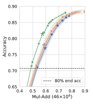
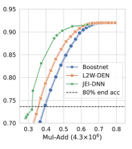
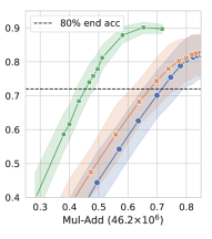
Figure 1: Accuracy vs Mul-Add of: Left CIFAR100 (t2t-14); Middle SVHN (t2t-7); and Right CIFAR100LT (t2t-14). The x-axes are scaled by the full model inference cost, Mul-Add ($IC^{L}$).

5.2 Baselines

We compare our proposal with the following baselines:

• BoostedNet (Yu et al., 2023) and L2W-DEN (Han et al., 2022b) are state-of-the-art benchmarks with architecture-agnostic training procedures for general-purpose networks.

• MSDNet (Huang et al., 2018) and RANet (Yang et al., 2020) are representative EEDN-tailored architectures. We additionally compare with the improved training procedures in (Yu et al., 2023) and (Han et al., 2022b).

To obtain the uncertainty metrics, we calibrate the predicted $\hat{\mathbf{p}}$ by first applying the post-calibration algorithm of temperature scaling from  (Guo et al., 2017) on the output logits using a validation set. Since all baselines also require a validation set to select gating thresholds, we split the validation set into two $\mathcal{V}=\mathcal{V}^{1}\cup\mathcal{V}^{2}$; $\mathcal{V}^{1}$ is used to compute the gating thresholds and $\mathcal{V}^{2}$ is used for hyperparameter tuning, early stopping, setting the conformal threshold, and calibrating the output.

5.3 Results

Observation 1:

Joint Training of the GMs and the IMs closes the train-test mismatch which leads to significant performance improvement.

Figure 1 depicts performance versus inference cost curves. Appendix 8.8 presents results on additional datasets and architectures. Focusing on the region exceeding $80\%$ of the end accuracy of the total network, our suggested approach significantly outperforms the baselines for all datasets. Outside of that range, it is on par or better. Moreover, the $95\%$ confidence intervals around the mean of the accuracy of our proposed approach (shaded areas) are significantly tighter. The CIs of all methods are wider for CIFAR100-LT. The imbalance leads to noisier prediction, which makes it particularly challenging for the baselines. To provide further insight into why our model outperforms the baselines, we analyze the results in the subsequent sections. Appendix 8.6 provides an ablation study which demonstrates the value of learnable gates and joint training.

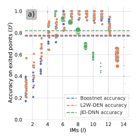
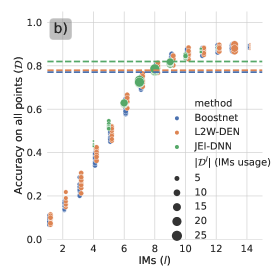
Figure 2: Decomposition of the contributions of the IMs to the final accuracies (depicted by dotted lines) for CIFAR100. The operational point is marked by a star in the left panel of Figure 1. a) Accuracy of each IM, $f^{l}_{\theta}$, evaluated only on their exited samples ($\mathcal{D}^{l}$). b) Accuracy of each IM, $f^{l}_{\theta}$, on the full dataset $\mathcal{D}$. The size of a circle is proportional to the number of samples exited for a trial.

Observation 2:

Training the GMs leads to a better gate selection.

Because our GMs are jointly trained with the IMs and take into account the cost of inference, the GMs can avoid poorly performing gates or gates that provide only marginal performance improvement. Figure 2 shows which gates are selected for exit by our proposed method (JEI-DNN) and the baselines. We see that JEI-DNN avoids using early IMs altogether and focuses on IMs 5 to 10. The joint training approach thus effectively addresses the EEDN placement task. Rather than employing fewer more capable, complex GMs and IMs selecting where to place them, as in (Li et al., 2023), our approach introduces very simple, lightweight GMs and IMs, and learns to focus on the IMs that can perform satisfactorily for a given inference budget. In contrast, the threshold GMs employed by the baselines lead to more evenly distributed exits. Since the threshold GMs make decisions by thresholding confidence metrics derived from predicted probabilities, it is more difficult to avoid exiting at early poorly performing IMs (these IMs are overly-confident for some samples).

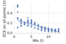
Figure 3: ECE of the IMs averaged over all baselines on all datasets with t2t-7.

Moreover, the thresholding approach implicitly relies on the assumption that the IMs are well calibrated, which cannot be guaranteed (Guo et al., 2017; Minderer et al., 2021). Experimentally, we verify that it is not the case and that calibration is positively correlated with the depth of the IMs (see Figure 3). Consequently, calibration is also correlated with accuracy, which is in line with the findings of Minderer et al. (2021)). A poor calibration leads to inaccurate predicted probabilities, which introduces noise in the inputs to the threshold GM. As a result, the exit selection is also more variable, leading to a less predictable accuracy-IC trade-off (as exhibited by the much wider CIs in Figure 1).

Observation 3:

Better gate selection concentrates training on better IMs.

Figure 2(b) highlights that the improvement of our model does not come from IMs that are superior over all of the training data. Baseline and JEI-DNN IMs perform similarly. The improvement in IC-accuracy trade-off is explained by the trend of IM accuracies in conjunction with IM usage. JEI-DNN exits very few samples at IMs 1-4 and 11-14. The early IMs are too inaccurate. The accuracy gain achieved by postponing exit to late IMs (11-14) is not justified by the increased inference cost.

The GMs must be able to accurately direct easier samples to earlier IMs. JEI-DNN clearly achieves this. For IMs 6-8, where most samples exit, the accuracy is higher over exiting samples (Fig. 2(a)) than all samples (Fig. 2(b)). By contrast, for gates 9-10, where only a few challenging samples exit, the exit accuracy is lower. For JEI-DNN, the most challenging samples exit at gates 9-11; for the baselines, they exit at gate 13. Despite having access to less informative features, JEI-DNN achieves a better average accuracy for these challenging samples at considerably lower inference cost.

Observation 4:

Learnable GMs leads to better uncertainty characterization capability

Fig. 4(a) highlights that even with post-calibration, the baselines’ predicted probabilities remain extremely poorly calibrated. JEI-DNN’s calibration is much better and the calibration error correlates negatively with accuracy. This is desirable; a higher inference cost should lead to better accuracy and better calibration. When the baselines provide more accuracy, the calibration error is much worse. This disparity has two causes: (i) JEI-DNN refrains from using the early, worst-calibrated gates (Fig. 3); (ii) the baselines must increase the GM thresholds to achieve higher accuracy, but this leads to a bias — samples only exit if the predictions are very confident.

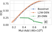
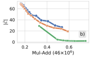
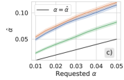
Figure 4: Uncertainty metrics on CIFAR-100 (t2t-14). a) ECE vs Mul-Add. b) Inefficiency vs Mul-Add for an empirical coverage bounded by $1-\hat{\alpha}\geq 95\%$ on CIFAR-100 (t2t-14). c) Average empirical $\hat{\alpha}$ vs requested $\alpha$. Appendix 8.8 presents results on other datasets and architectures.

We now consider conformal intervals. These should circumvent the threshold GM bias as they are derived via a validation set and have probabilistic guarantees. Fig. 4(b) shows that JEI-DNN offers significantly tighter conformal intervals $|\bar{\mathcal{C}|}$ for a given constraint on empirical coverage $\hat{\alpha}$. The empirical coverage values for JEI-DNN are also closer to the requested coverages $\alpha$ (see Fig. 4(c)).

Observation 5:

JEI-DNN using a fixed backbone outperforms dedicated EEDN architectures

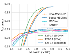
Figure 5: Comparison of T2T-ViT-14 and early-exit baselines on CIFAR-100. Results with * were taken from Han et al. (2022b).)

We now compare with state-of-the-art dedicated EEDN approaches that employ a trainable backbone. We select MSDNet (Huang et al., 2018), RANet (Yang et al., 2020), BoostedNet (Yu et al., 2023), and L2W-DEN (Han et al., 2022b) as representative models. Figure 5 shows that JEI-DNN with a T2T-ViT-14 backbone achieves much better accuracy while keeping the inference cost low. We achieve an accuracy of 82% for 22% of the inference cost of the full trainable backbone architectures. By contrast, the trainable architectures can only achieve an accuracy of 73% at this cost. However, in the very low-cost regime, dedicated EE architectures like MSDNet and RANet are able to maintain higher accuracy. By this point, however, the reduction in accuracy is severe.

6 Limitations

Although our proposal outperforms the baselines, both with respect to the accuracy-IC trade-off and uncertainty characterization, it has some drawbacks. First, since we must specify the inference cost parameter $\lambda$, we only obtain one accuracy/IC operational point per training. To obtain different values, we need to retrain the model with a changed $\lambda$ value. By contrast, the baseline methods that employ threshold GMs can modify the inference time after deployment by changing the threshold. Second, we cannot directly target a specific accuracy or inference cost. In practice, if there is a constraint on one of the metrics, we either must train multiple models, adjusting $\lambda$ until the constraint is met, or use an ad-hoc approach by applying different thresholds to the $g^{l}_{\phi}$ values. In summary, if the desired trade-off between inference cost and accuracy is likely to vary over time, and it is acceptable to sacrifice some accuracy, then the approach taken by the baselines would be preferable.

7 Conclusion

We have introduced a novel early-exit dynamic neural network architecture, JEI-DNN, that is compatible with off-the-shelf backbone architectures. By augmenting a backbone with lightweight, trainable gates and inference modules that are jointly optimized, we close the train-test gap, leading to better performance of inference modules. We show that this approach also outperforms state-of-the-art dedicated EEDN architectures. Furthermore, our approach provides significantly better uncertainty characterization. We show that the inference modules are better calibrated in the proposed JEI-DNN and tighter conformal intervals are obtained for a desired marginal coverage.

8 Appendix

8.1 Experiment details

8.1.1 Datasets

The CIFAR10 and CIFAR100 (Krizhevsky, 2009) datasets both consist of 60,000 $32\times 32$ coloured images. CIFAR10 has 10 classes and CIFAR100 has 100 classes. We follow a 75%-8.3%-16.6% train-validation-test split. The validation set is used for hyperparameter tuning and early-stopping. We also use the cropped-digit SVHN (Netzer et al., 2011) dataset which consists of 99,289 $32\times 32$ coloured images of house numbers where the target is the digit in the center. We use a 68.6%-5%-26.2% train-validation-test split. The CIFAR100-LT (long-tail) dataset consists of the regular CIFAR100 images but with imbalanced classes. We use an imbalance factor $if=100=\frac{|c_{\text{most common}}|}{|c_{\text{least common}}|}$. We follow the pre-processing procedure from  (Yuan et al., 2021). For all datasets, we use a training batch size of 64. We present 95$\%$ confidence intervals on the means of our results. These are generated using a bootstrap procedure over 10 trials derived by partitioning the test set into 10 subsets.

8.1.2 Experiment parameters

We use the Adam optimizer with a learning rate of $0.01$ with a weight decay of $5e{-}4$. We use a batch size of 64 for CIFAR10, CIFAR100 and CIFAR100LT, and a batch size of 256 for SVHN. We train until convergence using early stopping with a maximum of 15 epochs ($E$) for CIFAR10 and SVHN, 20 for CIFAR100LT and 30 for CIFAR100LT. For the number of warmup epochs $WE$, we perform a hyperparameter search over the range $\{1,\dots,E/2\}$.

8.1.3 Training time and memory usage

We report the average training time on a GPUx machine and number of parameters used for both architectures in Table 1. Overall, our approach takes a little longer to train and has a negligible number of additional parameters. Once trained, the baselines do have the advantage that heuristic adjustment of the gating threshold can achieve different IC/accuracy trade-offs.

Table 1: Memory usage and training time comparison. *We note that training time is to obtain a single IC/accuracy trade-off model (one point in our curve).

	JEI-DNN	Boostnet	L2W-DEN
T2T-7 (CIFAR10)
time* (min)	15	13	13
num. parameters	15.45K	15.42K	15.42K
T2T-14 (CIFAR100)
time* (min)	37	22	24
num. parameters	500.56K	500.50K	500.50K

8.1.4 Warm-up loss

We now provide a more thorough exposition of the warm-up phase which precedes the bi-level optimization phase. As mentioned, during warm-up we train all IMs in parallel on all samples. This is done to ensure that IMs have an acceptable accuracy and can potentially be chosen as exit points when we start training the gates. Earlier IMs have lower representational capacity and thus require more training. To that end, we increase the learning rate of earlier IMs using a simple position-based scaling. The warm-up loss for the $l^{th}$ IM can thus be written as:

$$\mathcal{L}_{warmup}^{l}=\frac{1}{N}\sum_{i=1}^{N}(L-l)lr_{0}\mathcal{L}^{CE}(y_{i},\hat{\mathbf{p}}_{\theta^{*}}^{l}(\mathbf{x}_{i})),$$ (17)

where $lr_{0}$ is set to 0.01 as a hyperparameter.

8.2 Inference Cost and Expected Calibration Error (ECE)

Inference cost:

Following BoostNet (Yu et al., 2023) and L2W-DEN (Han et al., 2022b), we measure the inference cost in terms of multiply-add operations (Mul-Add). For consistency, we base our implementation for computing the Mul-Adds on the code used by BoostNet, L2W-DEN and MSDNet (Huang et al., 2018). This implementation covers PyTorch modules that are used in MSDNet and we thus had to add support for modules used in the T2T-ViT architecture (Yuan et al., 2021). For these PyTorch modules we used the calculations from Electra (Clark et al., 2020). Since our training procedure directly relies on the inference cost (see equation 6) we measure the number of Mul-Adds at each exit before training, accounting for the layer of the backbone network, denoted $h^{l}$, the IM $f_{\theta_{l}}^{l}$ and the gate $g_{\phi_{l}}^{l}$. This value is treated as a function of $l$ that is constant across all samples exiting at layer $l$. That is, we ignore any possible decrease in Mul-Adds that might arise from sparsity in certain samples and thus use a worst-case scenario value that depends only on the network architecture and the input size. We can thus define the inference cost incurred for exiting at layer $l$:

$$\text{IC}^{l}=\sum_{k=1}^{l}\text{Mul-Add}(h^{k})+\text{Mul-Add}(f_{\theta_{k}}^{k})+\text{Mul-Add}(g_{\phi_{k}}^{k})$$ (18)

Tables 2 and 3 show the number of Mul-Adds at each exit of the base T2T-ViT-7 architecture on CIFAR10 and the base T2T-ViT-14 architecture on CIFAR100 respectively as well as the added Mul-Adds incurred from augmenting the backbone network with exit branches (IMs and gates) at every layer. We note that overall, this leads to an almost insignificant inference cost increase of less than 0.12% for the former and 1.12% for the latter. As a result of our very lightweight gate design, optimal branch placement is unnecessary.

Table 2: Comparison of the number of Mul-Adds per layer between the base T2T-ViT-7 backbone and JEI-DNN. The middle rows show the net increase due to augmenting with IMs and gates.

	$\text{IC}^{1}$	$\text{IC}^{2}$	$\text{IC}^{3}$	$\text{IC}^{4}$	$\text{IC}^{5}$	$\text{IC}^{6}$	$\text{IC}^{7}$
T2T ViT 7	5.533M	6.838M	8.145M	9.452M	10.759M	12.066M	13.502M
Cum. $\uparrow$ from IMs	+2570	+5140	+7710	+10280	+12850	+15420	+15420
Cum. $\uparrow$ from GMs	+96	+192	+288	+384	+480	+576	+576
JEI-DNN	5.534M	6.843M	8.153M	9.463M	10 .772M	12.082M	13.518M ($\uparrow 0.12\%$ )

Table 3: Comparison of the number of Mul-Adds per layer between the base T2T-ViT-14 backbone and JEI-DNN. The middle rows show the net increase due to augmenting with IMs and gates.

	$\text{IC}^{1}$	$\text{IC}^{2}$	$\text{IC}^{3}$	$\text{IC}^{4}$	$\text{IC}^{5}$	$\text{IC}^{6}$	$\text{IC}^{7}$
T2T ViT 14	7.249M	10.201M	13.152M	16.104M	19.056M	22.007M	24.959M
Cum. $\uparrow$ from IMs	+38.5K	+77K	+115.5K	+154K	+192.5K	+231K	+269.5K
Cum. $\uparrow$ from GMs	+906	+1812	+2718	+3624	+4530	+5436	+6342
JEI-DNN	7.289M	10.280M	13.271M	16.262M	19.253M	22.244M	25.235M
	$\text{IC}^{8}$	$\text{IC}^{9}$	$\text{IC}^{10}$	$\text{IC}^{11}$	$\text{IC}^{12}$	$\text{IC}^{13}$	$\text{IC}^{14}$
T2T ViT 14	27.911M	30.862M	33.814M	36.765M	39.717M	42.669M	45.848M
Cum. $\uparrow$ from IMs	+308K	+346.5K	+385K	+423.5K	+462K	+500.5K	+500.5K
Cum. $\uparrow$ from GMs	+7248	+8154	+9060	+9.96K	+10.87K	+11.78K	+11.78K
JEI-DNN	28.226M	31.217M	34.208M	37.199M	40.190M	43.181M	46.36M ($\uparrow 1.12\%$ )

Expected Calibration Error (ECE):

To estimate the ECE, we approximate the probability that $\hat{y}$ is correct given a predicted $\hat{p}^{\max}_{i}$. We evaluate the accuracy over a set of samples $ACC(\mathcal{Q})\triangleq\frac{1}{|\mathcal{Q}|}\sum_{i\in\mathcal{Q}}\mathbbm{1}[\hat{y}_{i}=y_{i}]$ and compare it to the average predicted probability $\bar{P}(\mathcal{Q})\triangleq\frac{1}{|\mathcal{Q}|}\sum_{i\in\mathcal{Q}}\hat{p}^{\max}_{i}$. The predicted probability values are sorted (denoting $\nu(j)$ as the sorting index such that $\hat{p}^{\max}_{\nu(j)}<\hat{p}^{\max}_{\nu(j+1)}$) and split into $B$ bins following (Guo et al., 2017) to approximate the ECE:

$$ECE\approx\sum^{B}_{b=1}\frac{|\mathcal{Q}_{b}|}{N}\Big{|}ACC(\mathcal{Q}_{b})-\bar{P}(\mathcal{Q}_{b})\Big{|}\quad\text{where }\mathcal{Q}_{b}=\{\nu(N(b-1)/B),\dots,\nu(Nb/B)\}\,.$$ (19)

8.3 Conformal intervals

In this section, we present other ways to obtain conformal intervals in the EEDN setting and show that they are all approximately equivalent. One simple approach is to consider all samples as a single group, ignoring where they exited. We can then use the entire validation set to select a single threshold. An alternative is to derive a different threshold for each IM. To do this, we partition the validation set into multiple smaller validation sets, one associated with each exit IM: $\mathcal{V}=\mathcal{V}^{1},\cup,\dots,\cup\mathcal{V}^{L}$. Each $val^{l}$ contains only the samples that exit at the $l$-th IM. In determining conformal interval threshold for the $l$-th IM, we then use only the samples in $\mathcal{V}^{l}$ and the predicted probabilities for that specific IM: $\hat{\mathbf{p}}_{\theta}^{l}(\mathbf{x}_{i})$. For each sample, we calculate a score $s_{i}=1-\hat{\mathbf{p}}_{\theta}(\mathbf{x}_{i}$). Given the set of scores $\{s_{i}\}$ and a coverage value $1-\alpha$, the conformal interval threshold value is determined by estimating the $1-\alpha$ percentile of $\{s_{i}\}$.

We construct four methods by combining different choices:

• General : We ignore the gating and use the entire validation set to obtain a single $\tau^{\mathcal{V},\alpha}$ value. We use this common threshold to generate the conformal sets for every exit IM. The score value for a given sample is derived from the predicted probabilities of its selected exit gate.

• IMs : We compute one threshold value per gate, but we use the entire validation set $\mathcal{V}$. The scores used to compute the threshold for the $l$-th IM are derived from $\hat{\mathbf{p}}_{\theta}^{l}(\mathbf{x}_{i})$. In this computation, we do not take any account of where a sample exits.

• Strict gating : A strict version of what we used in our experiments. We compute one threshold value per IM, using only the samples in the validation set associated with that IM. We derive the score function using $\hat{\mathbf{p}}_{\theta}^{l}(\mathbf{x}_{i})$. If no samples in the validation set are assigned to a specific IM, i.e; $|\mathcal{V}^{l}|=0$, we set $\tau_{l}^{\mathcal{V}^{l},\alpha}=0$.

• Gated: The version used to produce the experimental results in the paper. We use the strict gating approach, but if $|\mathcal{V}^{l}|<20$, we set $\tau_{l}=\tau^{\mathcal{V},\alpha}$, where $\tau^{\mathcal{V},\alpha}$ is derived using the General gating approach above.

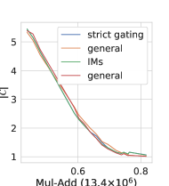
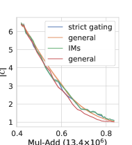
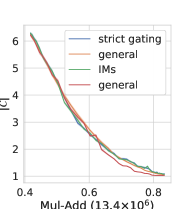
Figure 6: Inefficiency vs Mul-Add on CIFAR10 (t2t-7) of the conformal intervals obtained from the different methods. (Left) JEI-DNN, Middle Boostnet and Right L2W-DEN. The x-axis are scaled by the inference cost of the full model Mul-Add ($IC^{L}$).

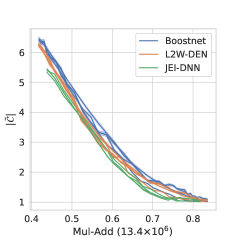
Figure 7: The conformal intervals obtained from all the different methods, for CIFAR10 t2t-vit-7.

Figure 6 shows that all methods are approximately equivalent for each baseline. Figure 7 shows that JEI-DNN achieves the smallest inefficiency for CIFAR10 t2t-vit-7, irrespective of the method chosen to construct confidence intervals. Similar results are obtained for the other datasets. To ensure that the comparison is meaningful, we report the smallest average inefficiency with an empirical coverage that exceeds the targeted coverage $1-\alpha$. To do this, for a targeted $\alpha=0.05$, we compute the conformal intervals from multiple thresholds, obtained by slowly decreasing the target $\alpha$: $\{\tau^{\alpha=0.05},\tau^{\alpha=0.045},\dots\}$ until the empirical coverage is above our target: $1-\hat{\alpha}>1-\alpha$. We then report the inefficiency at that empirical coverage.

8.4 Surrogate loss

In this section, we provide the connection between the surrogate problem we introduced for training the $\phi$s and the $\mathcal{L}^{out}$ as defined in equation 12:

$$\phi^{*}=\operatorname*{arg\,min}_{\phi}\mathcal{L}^{out}\triangleq\operatorname*{arg\,min}_{\phi}\frac{1}{N}\sum^{N}_{i=1}\sum^{L}_{l=1}C^{l}_{\theta^{*}(\phi)}P_{\phi}(G=l|\mathbf{x}_{i}).$$ (20)

We prove that if there exist a solution $\phi^{\prime}$ s.t. the associated $P_{\phi^{\prime}}(G=l|\mathbf{x}_{i})$s can be equal to each $P^{\prime}_{i}$ that minimizes:

$$P^{\prime}_{i} =\operatorname*{arg\,min}_{P}\sum^{L}_{l=1}C^{l}_{\theta^{*}(\phi)}P^{l}_{i},(\text{ with }\sum^{L}_{l=1}P_{i}^{l}=1,P_{i}^{l}>0)\quad\forall i\in[N],$$ (21)

then we can prove that $\phi^{\prime}$ will also be an optimal solution for our surrogate problem.

That is, $\phi^{\prime}$ also minimizes:

$$\frac{1}{N}\sum^{N}_{i=1}\sum^{L}_{l=1}\mathcal{L}^{CE}(t_{i}^{l},g^{l}_{\phi}(\mathbf{c}_{i}^{\leq l})),$$ (22)

where $t^{l}_{i}=0$ for $l<l^{*}$, $t^{l}_{i}=1$ for $l\geq l_{i}^{*}$, and $l^{*}=\operatorname*{arg\,min}_{l\in L}C^{j}_{\theta^{*}(\phi)}$.

For a given sample $i$, in order to minimize $\sum^{L}_{l=1}C^{l}_{\theta^{*}(\phi)}P^{l}_{i}$, we need to allocate all the probability mass of $P$ to the gate $l^{*}$ with the lowest cost. That is:

$$P^{\prime l}_{i}=\begin{cases}1\,\,\text{ if }\,\,l=l^{*}=\operatorname*{arg\,min}_{j}C^{j}_{\theta^{*}(\phi)}\\ 0\,\,\,\text{ o.w.}\end{cases}$$ (23)

Now provided that there exist a $\phi^{\prime}$ s.t. $P_{\phi^{\prime}}(G=l|\mathbf{x}_{i})=P^{\prime l}_{i}\,\forall i$, then $\phi^{*}=\phi^{\prime}$.

Now given that $P_{\phi^{\prime}}(G=l|\mathbf{x}_{i})=P^{\prime l}_{i}$, we can show that the associated gates $g^{l}_{\phi^{\prime}}$ have to satisfy:

$$g^{l}_{\phi^{\prime}}=\begin{cases}1\text{ if }l=\operatorname*{arg\,min}_{j}C^{j}_{\theta^{*}(\phi)\,,}\\ 0\text{ if }l<\operatorname*{arg\,min}_{j}C^{j}_{\theta^{*}(\phi)\,.}\end{cases}$$ (24)

Proof:

• For the trivial case where $l^{*}=1$, if $g^{1}_{\phi^{\prime}}=1$, then $P_{\phi^{\prime}}(G=1|\mathbf{x}_{i})=1$ by definition of $g^{1}_{\phi^{\prime}}(\mathbf{c}^{1})$ and $P_{\phi^{\prime}}(G=l|\mathbf{x}_{i})=min(g^{l}_{\phi}(\mathbf{c}_{i}^{\leq l}),0)=0$ for $l>1$.

• Suppose $l^{*}>1$, then $g^{l}_{\phi^{\prime}}=0$ for all $l<l^{*}$. This results in $P_{\phi^{\prime}}(G=l|\mathbf{x}_{i})=min(0,1-\sum^{l}_{j=1}0)=0$. Once we reach $g^{l*}_{\phi^{\prime}}=1$, this results in $P_{\phi^{\prime}}(G=l^{*}|\mathbf{x}_{i})=min(1,1-\sum^{l^{*}-1}_{j=1}0)=1$ and $P_{\phi^{\prime}}(G=l|\mathbf{x}_{i})=min(g^{l}_{\phi}(\mathbf{c}_{i}^{\leq l}),1-1)=0$. This concludes the proof.

Hence, since the optimized gates $g_{\phi^{\prime}}^{l}$ are given by  equation 24 which corresponds to the solution of our surrogate tasks, we have shown that those $\phi^{\prime}$ would be shared as the solution of both problems.

8.5 Algorithm

Algorithm 1 Training

1:  Input: num. of gates $L$, cost importance $\lambda$ parameter, num of epochs $E$, num of warm-up epochs $WE$, bilevel switch count bi_switch

2:  STATE=WARMUP

3:  for $we$ in $\{1,\dots,WE\}$ do

4:     for $\mathbf{x}_{i},y_{i}$ in batch do

5:        for $l$ in $\{1,\dots,L\}$ do

6:           $\mathcal{L}^{l}_{\theta_{l}}(x)=CE(p^{l}_{\theta}(x),y)$ (optimize each IM)

7:           Update the $\theta_{l}$ parameters

8:        end for

9:     end for

10:  end for

11:  STATE=GATE

12:  for $e$ in $\{WE,\dots,E\}$ do

13:     for $\mathbf{x}_{i},y_{i}$ in batch do

14:        if STATE = CLASSIFIER then

15:           Get probability of exiting at each gate $l$: $P_{\phi}(G=l|\mathbf{x}_{i})$

16:           Optimize the weighted loss $\mathcal{L}^{in}_{\theta}=\sum^{L}_{l=1}P_{\phi}(G=l|\mathbf{x}_{i})\mathcal{L}^{CE}(y_{i},\hat{\mathbf{p}}_{\theta,i}^{l})$

17:        else if STATE = GATE then

18:           Compute the inference cost at each gate l: $IC_{\text{norm}}^{l}$

19:           Compute the accuracy cost at each gate l: $\mathcal{L}^{CE}(y_{i},\hat{\mathbf{p}}_{\theta^{*},i}^{l})$

20:           Store the total cost of that gate: $C^{l}_{\theta^{*}(\phi)}=\Big{(}\mathcal{L}^{CE}(y_{i},\hat{\mathbf{p}}_{\theta^{*},i}^{l})+\lambda IC_{\text{norm}}^{l}\Big{)}$

21:           Compute the best gate $l*=\operatorname*{arg\,min}_{l}C^{l}_{\theta^{*}(\phi)}$ )

22:           Optimize $\mathcal{L}^{out}_{\phi}=\sum^{L}_{l=1}\frac{\partial\mathcal{L}^{CE}(t^{l}_{i},g^{l}_{\phi}(\mathbf{c}_{i}^{\leq l}))}{\partial\phi}$ ( equation 16)

23:        end if

24:        if batch idx = bi_switch then

25:           switch from STATE GATE to CLASSIFIER or from STATE CLASSIFIER to GATE

26:        end if

27:     end for

28:  end for

8.6 Ablation study

To verify that our joint training procedure is needed, we conduct an ablation study on the CIFAR10 dataset where we adapt our algorithm to the two decoupled settings:

1. Learnable GMs, fixed IMs: We use the same warm-up procedure, but avoid bi-level optimization, i.e., after warm-up we only optimize the gates’ parameters, $\phi$. We follow Algorithm 1 exactly, but never enter the $CLASSIFIER$ state. We train for the same total number of epochs.

2. Threshold GMs: We also adapt our algorithm to the other setting of threshold GMs. We remove the learnable gates from the architecture. We first train the IMs on all the data and then use the threshold gating algorithm used by Yu et al. (2023) and Han et al. (2022b).

The importance of joint training is illustrated Figure 8. The Learnable GMs, fixed IMs approach is less stable but slightly outperforms the Threshold GMs approach.

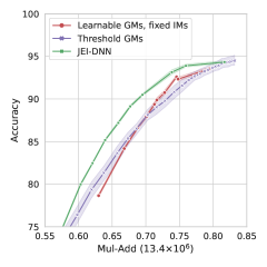
Figure 8: Ablation study on CIFAR10 (t2t-7). Jointly training the GMs and IMs is crucial; both decoupled approaches result in a performance decline.

8.7 Optimization of $\mathcal{L}^{in}$

The complete gradient to optimize the inner gradient of our bi-level formulation is given in equation 14:

$$\frac{\partial\mathcal{L}^{in}}{\partial\theta}=\frac{1}{N}\sum^{N}_{i=1}\sum^{L}_{l=1}\frac{\partial\mathcal{L}^{CE}(y_{i},\hat{\mathbf{p}}_{\theta}^{l}(\mathbf{x}_{i}))}{\partial\theta}P_{\phi}(G=l|\mathbf{x}_{i})+\frac{\partial G_{\phi}(m(\theta,\mathbf{x}_{i}))}{\partial\theta}C^{l}_{\theta(\phi)}\,$$ (25)

In our methodology, we mention that in practice, we ignore the right term of the gradient, and approximate the gradient using the term that corresponds to the gradient of a weighted cross entropy loss:

$$\frac{\partial\mathcal{L}^{in}}{\partial\theta} =\frac{1}{N}\sum^{N}_{i=1}\sum^{L}_{l=1}\frac{\partial\mathcal{L}^{CE}(y_{i},\hat{\mathbf{p}}_{\theta}^{l}(\mathbf{x}_{i}))}{\partial\theta}P_{\phi}(G=l|\mathbf{x}_{i})+{\color[rgb]{1,0,0}\frac{\partial G_{\phi}(m(\theta,\mathbf{x}_{i}))}{\partial\theta}C^{l}_{\theta(\phi)}}\,$$ (26)

$$\frac{\partial\mathcal{L}^{in}}{\partial\theta} \approx\frac{1}{N}\sum^{N}_{i=1}\sum^{L}_{l=1}\frac{\partial\mathcal{L}^{CE}(y_{i},\hat{\mathbf{p}}_{\theta}^{l}(\mathbf{x}_{i}))}{\partial\theta}P_{\phi}(G=l|\mathbf{x}_{i}).$$ (27)

We made that decision following our observation that both approaches yield comparable outcomes, but opting for the complete gradient leads to a slower convergence. We denote the JEI-DNN version using the full gradient equation 26 as JEI-DNN-FULL. Figure 9 shows the test accuracy of both models during training; we can see that both reach the same test accuracy, but that JEI-DNN reaches it considerably faster.

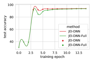
Figure 9: Test accuracy during training of both our proposed JEI-DNN and JEI-DNN-FULL.

8.8 Additional Results

We include additional performance versus inference cost curves in Figure 10, additional calibration versus inference cost curves in Figure 11 and inefficiency versus inference cost curves in Figure 12. The same trends as presented in the main paper can be observed.

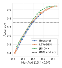
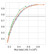
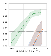
Figure 10: Accuracy vs Mul-Add of (Left) CIFAR10 (t2t-7), Middle CIFAR10 (t2t-14) and Right CIFAR100LT (t2t-7). The x-axes are scaled by the inference cost of the full model Mul-Add ($IC^{L}$).

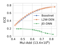
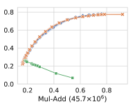
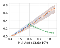
Figure 11: Calibration error vs Mul-Add of (Left) CIFAR10 (t2t-7), Middle CIFAR10 (t2t-14) and Right CIFAR100LT (t2t-7). The x-axes are scaled by the inference cost of the full model Mul-Add ($IC^{L}$).

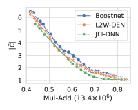
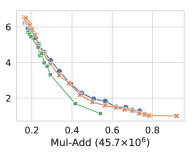
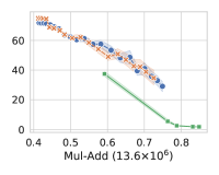
Figure 12: Inefficiency vs Mul-Add of (Left) CIFAR10 (t2t-7), Middle CIFAR10 (t2t-14) and Right CIFAR100LT (t2t-7). The x-axes are scaled by the inference cost of the full model Mul-Add ($IC^{L}$).

8.9 Uncertainty statistics

In this section we provide details concerning the uncertainty statistics that are used as input to our gate functions $g_{\phi}$. We represent the gate input as $m(\theta,\mathbf{x}_{i})=[\hat{p}^{max}_{i}(\mathbf{x}_{i}),h(\mathbf{x}_{i}),h_{pow}(\mathbf{x}_{i}),mar(\mathbf{x}_{i})]^{T}$ where:

• $\hat{p}^{max}_{i}(\mathbf{x}_{i})=\max(\mathbf{\hat{p}}_{i})$ is the maximum predicted probability;

• $h(\mathbf{x}_{i})=\sum_{k}\hat{\mathbf{p}}^{l,(k)}_{\theta,i}\log{\hat{\mathbf{p}}^{l,(k)}_{\theta,i}}$ is the entropy of the predictions;

• $h_{pow}(\mathbf{x}_{i})=\sum_{k}\tilde{\mathbf{p}}^{l,(k)}_{\theta,i}\log{\tilde{\mathbf{p}}^{l,(k)}_{\theta,i}}$ where $\tilde{\mathbf{p}}^{l,(k)}_{\theta,i}=\frac{(\hat{\mathbf{p}}^{l,(k)}_{\theta,i})^{2}}{\sum_{k^{\prime}}(\hat{\mathbf{p}}^{l,(k^{\prime})}_{\theta,i})^{2}}$ are scaled predictions (temp. = $0.5$);

• $mar(\mathbf{x}_{i})=p_{i}^{*}-p_{i}^{\prime}$ for $k_{i}^{*}=\operatorname*{arg\,max}_{k}\hat{\mathbf{p}}^{l,(k)}_{\theta,i}$, $p_{i}^{*}=\hat{\mathbf{p}}^{l,(k_{i}^{*})}_{\theta,i}$, and $p_{i}^{\prime}=\max_{k^{\prime}\neq k_{i}^{*}}\hat{\mathbf{p}}^{l,(k^{\prime})}_{\theta,i}$. This is the difference between the two most confident predictions.

8.10 Related work

In this appendix, we provide a more extensive and detailed discussion of related work, touching on some topics that are more tangentially related.

Architectures with threshold GMs

The majority of the literature on early-exit neural networks has primarily focused on designing architectures that are amenable to efficient and effective early-exit. Generally, in these approaches, the decision to exit at an earlier branch is taken by comparing confidence scores extracted from the IMs to predetermined thresholds.

The idea is first introduced by BranchyNet (Teerapittayanon et al., 2016), which augments a network with early-exit branches and trains the augmented model end-to-end, by summing a weighted loss of all IMs. Training the whole network end-to-end can bring complications as earlier IMs negatively impact the performance of later IMs. With this in mind, MSDNet (Huang et al., 2018) uses dense connections to reduce the influence of early IMs on later layers. The performance of earlier IMs is also improved by using representations of varying scales to train with coarser features. In RANNet (Yang et al., 2020), spatial redundancy of the input is exploited, with higher resolutions used only for the more difficult samples. In SDN (Kaya et al., 2019), off-the-shelf networks are augmented with intermediate IMs. Two training schemes are explored: freezing the backbone while training only the early exit branches or training the full network. The experimental results suggest that training the full network works better since the frozen backbone is optimized for the last layer. The interference of the early-exit branches on later layers is addressed via a weighted loss scheme with weights that depend on the position of the exit.

Another line of work has investigated ways of improving the training and performance of EE architectures by tackling the issue of conflicting gradient updates on the shared backbone parameters. These arise because the training procedure is attempting to simultaneously optimize multiple different exits. In IMTA (Li et al., 2019), the gradients computed when optimizing the intermediate IMs are rescaled based on their position in the network to ensure they have a bounded scale, reducing their variance. Additionally, knowledge distillation is employed to help earlier IMs learn from deeper ones. Meta-GF  Sun et al. (2022) also addresses conflicting gradient updates, but rather than using position-based rescaling, the scaling factors are learnt via a meta-learning formulation. The motivation is that in large over-parameterized models, certain parameters of the backbone are more relevant to some exits than others. Therefore, Meta-GF takes into account each parameter’s influence on the various exits before scaling the respective gradients.

Other research efforts have focused on customizing EEDNs to a specific type of backbone architecture. Wu et al. (2018) introduced an EEDN architecture customized for Residual networks, while Chen et al. (2018) did the same for CNNs.

Fundamentally, all these studies rely on confidence score thresholds that are set as hyperparameters to decide whether to early-exit. Most recent EEDN advances fall into this category of a dedicated architecture paired with either threshold GMs (Wang et al., 2020; Han et al., 2023b; Wang et al., 2021; Chen et al., 2023b) or other types of fixed gating mechanisms (Qian et al., 2022).

While most of these studies concentrate on image classification tasks, EEDNs have also seen expansion into other domains, including language models (Zhou et al., 2020; Schuster et al., 2022), as well as video frame classification (Seon et al., 2023).

EEDN research efforts have also explored how to fully leverage the additional computations performed by the previous gates and inference modules (Jiang & Mu, 2021; Wolczyk et al., 2021). For example, Wolczyk et al. (2021); Liu et al. (2022) and Passalis et al. (2020) all combine the outputs of the IMs using ensemble methods to enhance performance. Similarly, Qendro et al. (2021) also employ ensembling of IMs but target the uncertainty characterization of the overall network rather than inference cost.

Learnable GM; pre-trained and frozen backbone and IMs

Differing from the dedicated architecture and threshold GMs methods described above, another class of EEDN treats the IMs and backbone architecture as a fixed, frozen component, and focuses on training the GMs. In some cases, the pretraining of the IMs is included in the methodology. In (Bolukbasi et al., 2017), the learning is performed in two separate phases. First, the IMs are trained with the full training set and then the IMs are frozen and the gates are trained. The gates are trained sequentially starting from the deepest layer to the shallowest, allowing the gate training objective to be defined recursively. In EPNet (Dai et al., 2020) the task of training the gates after freezing the IMs is formulated as a Markov decision process. The methodology involves designing a substantial, trainable neural network of multiple layers for the gate mechanism. This was critized by following works as being wasteful, imposing an unacceptable inference overhead. PTEENet(Lahiany & Aperstein, 2022) parameterizes the gates and directly learns the exit decisions using sigmoid neural networks. EENet (Ilhan et al., 2023) adopts a different strategy by formulating the early-exit policy as a multi-objective optimization problem. Karpikova et al. (2023) design learnable gates, and specifically focus on confidence metrics tailored to images. Finally, there are tangential works such as (Li et al., 2023) that consider the related problem of optimizing gate placement for energy efficiency.

All of these models learn gating functions after having trained and frozen the IMs at every branch. While this two-phase procedure simplifies training, it ignores the coupling between gates and IMs — the gating decisions change the distributions of samples presented to the IMs, implying that parameters should be re-learned.

Addressing the train-test mismatch

Two recent works have proposed architecture-agnostic training procedures to address the aforementioned train-test mismatch. In BoostNet (Yu et al., 2023), the training procedure is inspired by gradient boosting. Prediction reweighting is employed so that deeper IMs are trained with prediction reweighting to induce an emphasis on samples that are incorrectly classified by the earlier IMs. Han et al. (2022b) cast the problem as a meta-learning task where a weight prediction network (WPN) is trained jointly with the early-exit network to predict the most likely exit of a sample. The predictions of the WPN are used to assign weights to the losses of the different IMs. Consequently, easy samples should have a reduced influence on deeper IMs while harder samples contribute more to their training. This architecture is related to ours but the training procedures differ in multiple important ways. Most importantly, we do not rely directly on thresholding uncertainty metrics for early exiting. We show that the uncertainty metrics are not a good proxy for accuracy for earlier IMs due to miscalibration. In practice, the inclusion of the weight prediction network does not close the train-test gap because it is trained using poorly calibrated labels. By jointly training the IMs and the GMs via bi-level optimization, our approach provides more reliable uncertainty characterization.

Chen et al. (2020) propose a fully trainable architecture featuring a learnable policy component that is responsible for determining the number of layers used for inference. Although Chen et al. (2020) do not target inference efficiency, their framework shares similarities with ours. The gating mechanism is modelled as a product of independent exiting events. However, the inference cost is not incorporated in the training objective. The gate exit distribution is controlled by an entropy regularization regularization; as a result, the procedure in (Chen et al., 2020) cannot be used to construct an effective EEDN.

This concludes our review of the most relevant EEDN contributions. We include a categorization of the works in Table 4. As is evident from the table, our approach is the only one that (i) can be applied to any layer-based off-the-shelf backbone network, without re-training the backbone; (ii) has learnable GMs and IMs; and (iii) jointly trains both the GMs and the IMs.

Sparsely-gated mixture-of-experts (MoE)

A closely related field to our problem setting is the Mixture of Experts (MoE) framework (Shazeer et al., 2017; Fedus et al., 2022; Du et al., 2022). In this framework, the network also employs a gating mechanism to make adaptive decisions based on the input it receives. However, in the MoE setting, the gating decisions are made across layers to incorporates multiple experts or weights (Shazeer et al., 2017; Du et al., 2022; Fedus et al., 2022). The goal is not to tailor inference time based on the input complexity but rather to enable the use of increasingly larger models by maintaining constant inference costs with sparse activation strategies. In this field, it is also considered an important problem to bridge the gap between the gating decisions and the inference modules (Gupta et al., 2022; Zhu et al., 2022). The interpretability potential of such architectures is also highlighted in (Pavlitska et al., 2022).

Online learning

In online learning with deep neural networks the aim is to jointly learn representations and a suitable architecture. However, given that the data is streamed serially during training, the optimal depth of the network may change as more data is accumulated. To address this, Sahoo et al. (2018) proposed to incorporate learnable GMs that produce a convex combination of IMs to construct a prediction that is a weighted average of all IM outputs and the final layer output. The GM training employs the hedge backpropagation algorithm proposed by Freund & Schapire (1997).

Table 4: Classification of EEDN problem settings and approaches. A tick mark indicates that a method is capable of providing this feature. Fixed backbone: The method can be applied to off-the-shelf backbones without re-training, i.e., it does not require a tailored EEDN backbone. Learnable GMs: The gates can be trained. Most methods use threshold GMs. Train IMs: The IMs are trained. Adaptive IM training: The training is adapted to different IMs, either by introducing weights or training with different subsets of the training data. Joint Training: Gate and IM parameters are jointly learned. * Indicates the baselines we include in our work.

Model	Fixed backbone	Learnable GMs	Train IMs	Adaptive IM Training	Joint Training
BranchyNet (Teerapittayanon et al., 2016)			✔
MSDNet (Huang et al., 2018)			✔
SDN (Kaya et al., 2019)	✔		✔
(Wang et al., 2020)			✔
(Wang et al., 2021)			✔
(Chen et al., 2023a)			✔
Han et al. (2023b)			✔
ReX: (Qian et al., 2022)			✔
IMTA (Li et al., 2019)			✔
Meta-GF (Sun et al., 2022)			✔
(Bolukbasi et al., 2017)		✔	✔
Predictive Exit (Li et al., 2023)	✔	✔
EPNet Dai et al. (2020)		✔	✔
PTEENet (Lahiany & Aperstein, 2022)	✔	✔
EENet (Ilhan et al., 2023)	✔	✔
Block-Dependent (Han et al., 2023a)			✔	✔
BoostedNet(Yu et al., 2023)	✔		✔	✔
L2W(Han et al., 2022b)	✔		✔	✔
JEI-DNN	✔	✔	✔	✔	✔

References

- Bolukbasi et al. (2017) Tolga Bolukbasi, Joseph Wang, Ofer Dekel, and Venkatesh Saligrama. Adaptive neural networks for efficient inference. In Proc. Int. Conf. Machine Learning. (ICML), 2017.
- Chen et al. (2023a) Can Chen, Xi Chen, Chen Ma, Zixuan Liu, and Xue Liu. Gradient-based bi-level optimization for deep learning: A survey. arXiv preprint: arXiv 2207.11719, 2023a.
- Chen et al. (2023b) Mengzhao Chen, Mingbao Lin, Ke Li, Yunhang Shen, Yongjian Wu, Fei Chao, and Rongrong Ji. CF-ViT: A general coarse-to-fine method for vision transformer. In Proc. of the AAAI Conf. on Artificial Intelligence, 2023b.
- Chen et al. (2020) Xinshi Chen, Hanjun Dai, Yu Li, Xin Gao, and Le Song. Learning to stop while learning to predict. In Proc. Int. Conf. Machine Learning. (ICML), 2020.
- Chen et al. (2018) Zhourong Chen, Yang Li, Samy Bengio, and Si Si. You look twice: Gaternet for dynamic filter selection in cnns. In Proc. IEEE/CVF Conf. on Computer Vision and Pattern Recognit. (CVPR), 2018.
- Chiang et al. (2021) Chang-Han Chiang, Pangfeng Liu, Da-Wei Wang, Ding-Yong Hong, and Jan-Jan Wu. Optimal branch location for cost-effective inference on branchynet. In Proc. IEEE Int. Conf. on Big Data (Big Data), 2021.
- Clark et al. (2020) Kevin Clark, Minh-Thang Luong, Quoc V. Le, and Christopher D. Manning. ELECTRA: Pre-training text encoders as discriminators rather than generators. In Proc. Int. Conf. on Learning Representations (ICLR), 2020.
- Dai et al. (2020) Xin Dai, Xiangnan Kong, and Tian Guo. EPNet: Learning to exit with flexible multi-branch network. In Proc. Int. Conf. on Inf. & Knowledge Management (CIKM), 2020.
- Deng et al. (2009) Jia Deng, Wei Dong, Richard Socher, Li-Jia Li, Kai Li, and Li Fei-Fei. Imagenet: A large-scale hierarchical image database. In Proc. IEEE/CVF Conf. on Computer Vision and Pattern Recognit. (CVPR), 2009.
- Du et al. (2022) Nan Du, Yanping Huang, Andrew M Dai, Simon Tong, Dmitry Lepikhin, Yuanzhong Xu, Maxim Krikun, Yanqi Zhou, Adams Wei Yu, Orhan Firat, Barret Zoph, Liam Fedus, Maarten P Bosma, Zongwei Zhou, Tao Wang, Emma Wang, Kellie Webster, Marie Pellat, Kevin Robinson, Kathleen Meier-Hellstern, Toju Duke, Lucas Dixon, Kun Zhang, Quoc Le, Yonghui Wu, Zhifeng Chen, and Claire Cui. GLaM: Efficient scaling of language models with mixture-of-experts. In Proc. Int. Conf. Machine Learning. (ICML), 2022.
- Fedus et al. (2022) William Fedus, Barret Zoph, and Noam Shazeer. Switch transformers: Scaling to trillion parameter models with simple and efficient sparsity. Jour. of Machine Learning Research, 23(120):1–39, 2022.
- Freund & Schapire (1997) Yoav Freund and Robert E Schapire. A decision-theoretic generalization of on-line learning and an application to boosting. J. Comp. System Sciences, 55(1):119–139, 1997.
- Guo et al. (2017) Chuan Guo, Geoff Pleiss, Yu Sun, and Kilian Q. Weinberger. On calibration of modern neural networks. In Proc. Int. Conf. Machine Learning. (ICML), 2017.
- Gupta et al. (2022) Shashank Gupta, Subhabrata Mukherjee, Krishan Subudhi, Eduardo Gonzalez, Damien Jose, Ahmed H. Awadallah, and Jianfeng Gao. Sparsely activated mixture-of-experts are robust multi-task learners. arXiv preprint: arXiv 2204.07689, 2022.
- Han et al. (2023a) Dong-Jun Han, Jungwuk Park, Seokil Ham, Namjin Lee, and Jaekyun Moon. Improving low-latency predictions in multi-exit neural networks via block-dependent losses. IEEE Transactions on Neural Networks and Learning Systems, pp. 1–9, 2023a.
- Han et al. (2022a) Y. Han, G. Huang, S. Song, L. Yang, H. Wang, and Y. Wang. Dynamic neural networks: A survey. IEEE Trans. on Pattern Analysis.; Mach. Intell., 44(11):7436–7456, 2022a.
- Han et al. (2022b) Yizeng Han, Yifan Pu, Zihang Lai, Chaofei Wang, Shiji Song, Junfen Cao, Wenhui Huang, Chao Deng, and Gao Huang. Learning to weight samples for dynamic early-exiting networks. In Proc. European Conf. on Computer Vision (ECCV), 2022b.
- Han et al. (2023b) Yizeng Han, Dongchen Han, Zeyu Liu, Yulin Wang, Xuran Pan, Yifan Pu, Chao Deng, Junlan Feng, Shiji Song, and Gao Huang. Dynamic perceiver for efficient visual recognition. In Proc, IEEE Int. Conf. on Computer Vision (ICCV), 2023b.
- Huang et al. (2018) Gao Huang, Danlu Chen, Tianhong Li, Felix Wu, Laurens van der Maaten, and Kilian Weinberger. Multi-scale dense networks for resource efficient image classification. In Proc. Int. Conf. on Learning Representations (ICLR), 2018.
- Ilhan et al. (2023) Fatih Ilhan, Ling Liu, Ka-Ho Chow, Wenqi Wei, Yanzhao Wu, Myungjin Lee, Ramana Kompella, Hugo Latapie, and Gaowen Liu. EEnet: Learning to early exit for adaptive inference. arXiv preprint: arXiv 2301.07099, 2023.
- Jiang & Mu (2021) Borui Jiang and Yadong Mu. Russian doll network: Learning nested networks for sample-adaptive dynamic inference. In Proc. Int. Conf. on Computer Vision Workshops (ICCVW), 2021.
- Karpikova et al. (2023) Polina Karpikova, Ekaterina Radionova, Anastasia Yaschenko, Andrei Spiridonov, Leonid Kostyushko, Riccardo Fabbricatore, and Aleksei Ivakhnenko. FIANCEE: Faster inference of adversarial networks via conditional early exits. In Proc. IEEE/CVF Conf. on Computer Vision and Pattern Recognit. (CVPR), 2023.
- Kaya et al. (2019) Yigitcan Kaya, Sanghyun Hong, and Tudor Dumitras. Shallow-deep networks: Understanding and mitigating network overthinking. In Proc. Int. Conf. Machine Learning. (ICML), 2019.
- Krizhevsky (2009) Alex Krizhevsky. Learning multiple layers of features from tiny images. Technical report, University of Toronto, 2009.
- Lahiany & Aperstein (2022) Assaf Lahiany and Yehudit Aperstein. PTEENet: Post-trained early-exit neural networks augmentation for inference cost optimization. IEEE Access, 10:69680–69687, 2022.
- Laskaridis et al. (2021) Stefanos Laskaridis, Alexandros Kouris, and Nicholas D. Lane. Adaptive inference through early-exit networks: Design, challenges and directions. In Proc. Int. Workshop on Embedded and Mobile Deep Learning, 2021.
- Li et al. (2019) Hao Li, Hong Zhang, Xiaojuan Qi, Ruigang Yang, and Gao Huang. Improved techniques for training adaptive deep networks. In Proc. IEEE/CVF International Conference on Computer Vision (ICCV), 2019.
- Li et al. (2023) Xiangjie Li, Chenfei Lou, Yuchi Chen, Zhengping Zhu, Yingtao Shen, Yehan Ma, and An Zou. Predictive exit: Prediction of fine-grained early exits for computation- and energy-efficient inference. In Proc. AAAI Conf. on Artificial Intell., 2023.
- Liu et al. (2022) Shiwei Liu, Tianlong Chen, Zahra Atashgahi, Xiaohan Chen, Ghada Sokar, Elena Mocanu, Mykola Pechenizkiy, Zhangyang Wang, and Decebal Constantin Mocanu. Deep ensembling with no overhead for either training or testing: The all-round blessings of dynamic sparsity. In Proc. Int. Conf. on Learning Representations (ICLR), 2022.
- Minderer et al. (2021) Matthias Minderer, Josip Djolonga, Rob Romijnders, Frances Hubis, Xiaohua Zhai, Neil Houlsby, Dustin Tran, and Mario Lucic. Revisiting the calibration of modern neural networks. In Proc. Adv. Neural Info. Process. Syst. (NeurIPS), 2021.
- Netzer et al. (2011) Yuval Netzer, Tao Wang, Adam Coates, Alessandro Bissacco, Bo Wu, and Andrew Y. Ng. Reading digits in natural images with unsupervised feature learning. In Proc. NIPS Workshop on Deep Learning and Unsupervised Feature Learning 2011, 2011.
- Passalis et al. (2020) Nikolaos Passalis, Jenni Raitoharju, Anastasios Tefas, and Moncef Gabbouj. Efficient adaptive inference for deep convolutional neural networks using hierarchical early exits. Pattern Recognition, 105, 2020.
- Pavlitska et al. (2022) Svetlana Pavlitska, Christian Hubschneider, Lukas Struppek, and J. Marius Zollner. Sparsely-gated mixture-of-expert layers for CNN interpretability. In Proc. Int. Joint Conf. on Neural Networks (IJCNN), 2022.
- Qendro et al. (2021) Lorena Qendro, Alexander Campbell, Pietro Lio, and Cecilia Mascolo. Early exit ensembles for uncertainty quantification. In Proc. of Machine Learning for Health, 2021.
- Qian et al. (2022) Xuwei Qian, Renlong Hang, and Qingshan Liu. Rex: An efficient approach to reducing memory cost in image classification. In Proc. AAAI Conf. on Artificial Intell., Jun. 2022.
- Sahoo et al. (2018) Doyen Sahoo, Quang Pham, Jing Lu, and Steven C. H. Hoi. Online deep learning: Learning deep neural networks on the fly. In Proc. Int. Joint Conf. Artificial Intell. (IJCAI), 2018.
- Scao et al. (2023) Teven Le Scao, Angela Fan, Christopher Akiki, Ellie Pavlick, Suzana Ilić, Daniel Hesslow, Roman Castagné, Alexandra Sasha Luccioni, François Yvon, Matthias Gallé, Jonathan Tow, Alexander M. Rush, Stella Biderman, Albert Webson, Pawan Sasanka Ammanamanchi, Thomas Wang, Benoît Sagot, Niklas Muennighoff, Albert Villanova del Moral, Olatunji Ruwase, Rachel Bawden, Stas Bekman, Angelina McMillan-Major, Iz Beltagy, Huu Nguyen, Lucile Saulnier, Samson Tan, Pedro Ortiz Suarez, Victor Sanh, Hugo Laurençon, Yacine Jernite, Julien Launay, Margaret Mitchell, and Colin Raffel. Bloom: A 176b-parameter open-access multilingual language model. arXiv preprint: arXiv 2211.05100, 2023.
- Schuster et al. (2022) Tal Schuster, Adam Fisch, Jai Gupta, Mostafa Dehghani, Dara Bahri, Vinh Q. Tran, Yi Tay, and Donald Metzler. Confident adaptive language modeling. In Proc. Adv. Neural Info. Process. Syst. (NeurIPS), 2022.
- Seon et al. (2023) J. Seon, J. Hwang, J. Mun, and B. Han. Stop or forward: Dynamic layer skipping for efficient action recognition. In Proc. IEEE/CVF Winter Conf. on Applications of Computer Vision (WACV), 2023.
- Shazeer et al. (2017) Noam Shazeer, Azalia Mirhoseini, Krzysztof Maziarz, Andy Davis, Quoc Le, Geoffrey Hinton, and Jeff Dean. Outrageously large neural networks: The sparsely-gated mixture-of-experts layer. In Proc. Int. Conf. on Learning Representations (ICLR), 2017.
- Sun et al. (2022) Yi Sun, Jian Li, and Xin Xu. Meta-GF: Training dynamic-depth neural networks harmoniously. In Proc. European Conf. on Computer Vision (ECCV), 2022.
- Teerapittayanon et al. (2016) Surat Teerapittayanon, Bradley McDanel, and H.T. Kung. Branchynet: Fast inference via early exiting from deep neural networks. In Proc. Int. Conf. on Pattern Recognition (ICPR), 2016.
- Wang et al. (2020) Yulin Wang, Kangchen Lv, Rui Huang, Shiji Song, Le Yang, and Gao Huang. Glance and focus: a dynamic approach to reducing spatial redundancy in image classification. In Proc. Adv. Neural Info. Process. Syst. (NeurIPS), volume 33, 2020.
- Wang et al. (2021) Yulin Wang, Rui Huang, Shiji Song, Zeyi Huang, and Gao Huang. Not all images are worth 16x16 words: Dynamic transformers for efficient image recognition. In Proc. Adv. Neural Info. Process. Syst. (NeurIPS), 2021.
- Wolczyk et al. (2021) Maciej Wolczyk, Bartosz Wójcik, Klaudia Bałazy, Igor T. Podolak, Jacek Tabor, Marek Śmieja, and Tomasz Trzcinski. Zero time waste: Recycling predictions in early exit neural networks. In Proc. Adv. Neural Info. Process. Syst. (NeurIPS), 2021.
- Wu et al. (2018) Zuxuan Wu, Tushar Nagarajan, Abhishek Kumar, Steven Rennie, Larry S Davis, Kristen Grauman, and Rogerio Feris. BlockDrop: Dynamic inference paths in residual networks. In Proc. IEEE/CVF Conf. on Computer Vision and Pattern Recognit. (CVPR), 2018.
- Yang et al. (2020) Le Yang, Yizeng Han, Xi Chen, Shiji Song, Jifeng Dai, and Gao Huang. Resolution adaptive networks for efficient inference. In Proc. IEEE/CVF Conf. on Computer Vision and Pattern Recognit. (CVPR), 2020.
- Yu et al. (2023) Haichao Yu, Haoxiang Li, Gang Hua, Gao Huang, and Humphrey Shi. Boosted dynamic neural networks. In Proc. AAAI Conf. on Artificial Intell., volume 37, 2023.
- Yuan et al. (2021) Li Yuan, Yunpeng Chen, Tao Wang, Weihao Yu, Yujun Shi, Zihang Jiang, Francis EH Tay, Jiashi Feng, and Shuicheng Yan. Tokens-to-token ViT: Training vision transformers from scratch on imagenet. In Proc, IEEE Int. Conf. on Computer Vision (ICCV), 2021.
- Zhou et al. (2020) Wangchunshu Zhou, Canwen Xu, Tao Ge, Julian McAuley, Ke Xu, and Furu Wei. BERT loses patience: Fast and robust inference with early exit. In Proc. Adv. Neural Info. Process. Syst. (NeurIPS), volume 33, 2020.
- Zhu et al. (2022) Jinguo Zhu, Xizhou Zhu, Wenhai Wang, Xiaohua Wang, Hongsheng Li, Xiaogang Wang, and Jifeng Dai. Uni-Perceiver-MoE: Learning sparse generalist models with conditional MoEs. In Proc. Adv. Neural Info. Process. Syst. (NeurIPS), 2022.