JWST MIRI/MRS Observations and Spectral Models of the Under-luminous Type Ia Supernova 2022xkq

Abstract

We present a JWST mid-infrared spectrum of the under-luminous Type Ia Supernova (SN Ia) 2022xkq, obtained with the medium-resolution spectrometer on the Mid-Infrared Instrument (MIRI) $\sim 130$ days post-explosion. We identify the first MIR lines beyond 14 $\mu$m in SN Ia observations. We find features unique to under-luminous SNe Ia, including: isolated emission of stable Ni, strong blends of [Ti II], and large ratios of singly ionized to doubly ionized species in both [Ar] and [Co]. Comparisons to normal-luminosity SNe Ia spectra at similar phases show a tentative trend between the width of the [Co III] 11.888 $\mu$m feature and the SN light curve shape. Using non-LTE-multi-dimensional radiation hydro simulations and the observed electron capture elements we constrain the mass of the exploding white dwarf. The best-fitting model shows that SN 2022xkq is consistent with an off-center delayed-detonation explosion of a near-Chandrasekhar mass WD (M_ej $\approx 1.37$ M_⊙) of high-central density ($\rho_{c}\geq 2.0\times 10^{9}$ g cm^-3) seen equator on, which produced M(⁵⁶Ni) $=0.324$ M_⊙ and M(⁵⁸Ni) $\geq 0.06$ M_⊙. The observed line widths are consistent with the overall abundance distribution; and the narrow stable Ni lines indicate little to no mixing in the central regions, favoring central ignition of sub-sonic carbon burning followed by an off-center DDT beginning at a single point. Additional observations may further constrain the physics revealing the presence of additional species including Cr and Mn. Our work demonstrates the power of using the full coverage of MIRI in combination with detailed modeling to elucidate the physics of SNe Ia at a level not previously possible.

1 Introduction

The use of Type Ia supernovae (SNe Ia) as cosmological distance indicators belies their diverse nature. Through the luminosity-width relation (Phillips, 1993), both bright, slow-declining and dimmer, fast-declining SN Ia can be standardized for cosmological analyses, which have revealed the accelerating expansion of the universe (Riess et al., 1998; Perlmutter et al., 1999). Spectroscopic diversity among SNe Ia has also been observed, with multiple schemes to understand this diversity, based solely on spectroscopic information (Branch et al., 2006; Wang et al., 2009), or combined photometric and spectroscopic measurements (Benetti et al., 2005), having been developed. Evidence suggests that much of the observed diversity originates from differences in the radioactive Ni mass (e.g. ⁵⁶Ni) (Nugent et al., 1995; Pinto & Eastman, 2000a, b), resulting in several sub-types of SNe Ia with unique photometric and spectroscopic properties including (but not limited to): 91T-like objects (Filippenko et al., 1992a; Phillips et al., 1992, 2022; Yang et al., 2022), 91bg-like objects (Filippenko et al., 1992b; Leibundgut et al., 1993; Galbany et al., 2019; Hoogendam et al., 2022) 02cx-like (aka SN Iax) (Li et al., 2003; Foley et al., 2013; Jha, 2017), and 03fg-like (formerly known as super-Chandrasekhar SNe Ia) (Howell et al., 2006; Hicken et al., 2007; Scalzo et al., 2010; Hsiao et al., 2020; Ashall et al., 2021).

A major outstanding question is whether individual SNe Ia subgroups (e.g under-luminous or 91bg-like objects) arise from different progenitor systems and/or explosion mechanisms (or particular combinations thereof) than other subgroups. SNe Ia are known to originate from the thermonuclear explosion of a carbon-oxygen (C/O) white dwarf (WD) in a multi-star system (Hoyle & Fowler, 1960; Bloom et al., 2012). The range of possible progenitor systems includes: the single degenerate (SD) scenario in which the companion is a main-sequence star or an evolved, non-degenerate companion such as a red giant or He-star (Whelan & Iben, 1973); the double degenerate scenario (DD) in which the companion is also a WD (Iben & Tutukov, 1984; Webbink, 1984), or a triple system in which at least two of the bodies are C/O WDs (Thompson, 2011; Kushnir et al., 2013; Shappee & Thompson, 2013; Pejcha et al., 2013).

Within the context of the above progenitor scenarios, multiple explosion mechanisms exist (e.g. Benz et al., 1990; Hoeflich & Khokhlov, 1996; Rosswog et al., 2009; Pakmor et al., 2012, 2013; Kushnir et al., 2013; Soker et al., 2013; García-Berro et al., 2017; Lu et al., 2021). Currently, two of the leading explosion models are the detonation of a sub-M_Ch WD or the explosion of a near-M_Ch WD. In sub-M_Ch explosions, He on the WD surface (which may be accreted from a degenerate or non-degenerate companion) detonates, driving a shockwave into the WD which triggers a second, interior detonations which disrupts the whole WD (Nomoto et al., 1984; Woosley & Weaver, 1994; Livne & Arnett, 1995; Hoeflich & Khokhlov, 1996; Shen et al., 2018; Polin et al., 2019; Boos et al., 2021). In contrast, for near-M_Ch explosions, H, He, and/or C material is accreted from a companion star (which may again be degenerate or non-degenerate) onto the surface of the WD, until compressional heating triggers an explosion near the WD center (Nomoto et al., 1976; Iben & Tutukov, 1984; Hoeflich & Khokhlov, 1996; Diamond et al., 2018). The flame front may propagate as either a deflagration, detonation, or both via a deflagration-to-detonation transition (Khokhlov, 1991; Hoeflich & Khokhlov, 1996; Gamezo et al., 2003; Poludnenko et al., 2019, DDT;).

Nebular-phase spectra of SNe Ia in the mid-infrared (MIR) are key to distinguishing between different explosion models. As the location of the photosphere is wavelength dependent, different spectral lines are revealed in the MIR (Meikle et al., 1993; Höflich et al., 2002a; Wilk et al., 2018) which are better at constraining the physics of SN explosions than their optical counterparts (Diamond et al., 2015, 2018). For example, the amount of stable Ni (e.g. ⁵⁸Ni) and other iron group elements (IGEs) serve as a direct indicator of the central density ($\rho_{c}$) at the time of explosion (Hoeflich & Khokhlov, 1996; Seitenzahl & Townsley, 2017; Blondin et al., 2022). Optical lines from stable Ni are only identified as weak components of heavily blended features (Maguire et al., 2018; Mazzali et al., 2020) and the 1.94 $\mu$m [Ni II] NIR line lies directly adjacent to (and often overlapping) a telluric region; making its identification difficult and sensitive to reduction methodology in high-quality data (Friesen et al., 2014; Dhawan et al., 2018; Diamond et al., 2018; Hoeflich et al., 2021). However, in the MIR, stable Ni can be seen even in low S/N observations (Gerardy et al., 2007; Telesco et al., 2015), with multiple strong lines in different ionization stages seen in high S/N JWST observations (Kwok et al., 2023a; DerKacy et al., 2023).

To date, the complete published sample of MIR nebular phase spectra of SNe Ia contains nine spectra of five normal luminosity objects, and one spectrum of a 2003fg-like SNe Ia. This data includes single epoch observations of SNe 2003hv, 2005df (Gerardy et al., 2007), and 2006ce (Kwok et al., 2023a) with the Spitzer Space Telescope; plus a JWST observation of the 03fg-like SN 2022pul (Siebert et al., 2023; Kwok et al., 2023b). Two time series data sets exist; four observations of SN 2014J with CarnariCam on the Gran Telescopio de Canarias (GTC) (Telesco et al., 2015), and two observations of SN 2021aefx (Kwok et al., 2023a; DerKacy et al., 2023) with the Low Resolution Spectrograph (Kendrew et al., 2015; Rigby et al., 2023, LRS;) mode of the Mid-Infrared Instrument (MIRI; Rieke et al., 2015, and references therein). All of these published MIR spectra have resolutions of R $\lesssim$ 200. With an average resolution R $\sim 2700$ from 5-25 $\mu$m, observations of SNe Ia with JWST/MIRI using the Medium Resolution Spectrograph (Rieke et al., 2015; Wells et al., 2015; Argyriou et al., 2023, MRS;) can make more precise measurements of the line velocities and line profiles, and provide coverage in the 14-25 $\mu$m region unobtainable with MIRI/LRS. To date, no spectral observations of SNe Ia from MIRI/MRS have been published in literature.

In this work, we present a medium-resolution nebular-phase spectrum of the under-luminous SN 2022xkq taken $\sim$ 130 days after explosion with MIRI/MRS. § 2 describes our observations and reduction procedures. Line identifications are made in § 3, and important aspects of the spectrum are characterized in § 4, including discussions of the differences in the MIR spectra of SN 2022xkq versus normal-luminosity SNe Ia observed at similar epochs. Interpretation of our observations with the use of radiative hydrodynamic models are presented in § 5. We summarize our results in § 6 and discuss the implications of this work in § 7. We conclude in § 8.

2 Observations

Table 1: Properties of SN 2022xkq and NGC 1784 .

Parameter	Value	Source
SN 2022xkq
R.A.	05h05m23s.70	(1)
Dec.	$-$11°52′56″.13	(1)
Last Non-Detection (MJD)	59864.25	(1)
Discovery (MJD)	59865.37	(1)
$t_{\rm exp}$ (MJD)	$59865.0\pm 0.3$	(2)
$t_{\rm max}$ (MJD)	$59879.03\pm 0.34$	(2)
$M_{B,{\rm max}}$ (mag)	$-18.01\pm 0.15$	(2)
$\Delta{\rm m_{15}(B)}$ (mag)	$1.65\pm 0.03$	(2)
sBV	$0.63\pm 0.03$	(2)
$E(B-V)_{MW}$ (mag)	$0.116\pm 0.002$	(3)
NGC 1784
R.A.	05h05m27s.10	(4)
Dec.	$-$11°52′17″.50	(4)
Morphology	SB(r)c	(4)
$v_{\rm helio}$ (km s-1)	$2291\pm 11$	(5)
$v_{\rm rot}$ (km s-1)	$41\pm 20$	(4)
$z$	0.0077	(5)
$\mu$	$32.46\pm 0.15$	(2)

Note. — Pearson et al. (2023) find negligible host extinction at the site of SN 2022xkq.

References. — (1) Janzen et al. (2022), (2) Pearson et al. (2023), (3) Schlafly & Finkbeiner (2011), (4) Ratay (2004), (5) Koribalski et al. (2004), (6) NED

2.1 Early Observations of SN 2022xkq

SN 2022xkq was discovered on 2022 October 13.4 UT (MJD=59865.4) by the Distance Less Than 40 Mpc Survey (Tartaglia et al., 2018, DLT40;), with a last non-detection on 2022 October 12.3 UT (MJD$=$59864.3). Initially classified as a Type I (Chen et al., 2022a) or Type Ic (Hosseinzadeh et al., 2022) supernova, further observations revealed SN 2022xkq to be a 91bg-like SN Ia (Chen et al., 2022b).

A detailed analysis of SN 2022xkq can be found in Pearson et al. (2023). We briefly summarize some of their key findings, with important measurements of SN 2022xkq and its host NGC 1784 shown in § 2. SN 2022xkq is a transitional SNe Ia similar to SNe 1986G (Phillips et al., 1987; Ashall et al., 2016b), 2005ke (Patat et al., 2012), 2007on, 2011iv (Gall et al., 2018; Ashall et al., 2018), and 2012ij (Li et al., 2022). SNooPy (Burns et al., 2011, 2014) fits to the early light curve show that SN 2022xkq has $\Delta{\rm m_{15}(B)}$ $=1.65\pm 0.03$ mag and s_BV $=0.63\pm 0.03$. Using Arnett’s Rule (Arnett, 1982; Arnett et al., 1985), the pseudo-bolometric light curves, and the peak bolometric luminosity, Pearson et al. (2023) derived a ⁵⁶Ni mass of $0.22\pm 0.03$ M_⊙ in SN 2022xkq. Early photometry revealed SN 2022xkq to be red in color, with a flux excess in the redder bands relative to power-law fits in the first few days after explosion. In addition, densely sampled spectra showed strong, persistent C lines (particularly C I $\lambda 1.069$ $\mu$m), similar to SN 1999by. Radio observations taken on 2022 October 15.9 with the Australia Telescope Compact Array (ATCA) found no radio emission at the site of SN 2022xkq, placing 3-$\sigma$ upper limits of 0.07 mJy at 5.5 GHz and 0.04 mJy at 9.0 GHz (Ryder et al., 2022).

The host galaxy of SN 2022xkq is NGC 1784, a barred spiral SB(r)c galaxy at a distance of roughly 31 Mpc (de Vaucouleurs et al., 1991; Pearson et al., 2023). SN 2022xkq is located near the edge of a weak spiral arm, 49″.91 W and 38″.63 S of the center of its host galaxy (see Figure 1 in Pearson et al., 2023). Underluminous SNe Ia are typically found in older stellar populations, and thus more likely to occur in elliptical galaxies (Hamuy et al., 1996; Branch et al., 1996; Howell, 2001; Sullivan et al., 2010; Ashall et al., 2016a; Nugent et al., 2023); although old stellar populations can also be found in late-type spirals such as NGC 1784. Interestingly, the under-luminous SN 1999by was also discovered in a late-type spiral (Howell, 2001; Höflich et al., 2002b; Garnavich et al., 2004), and shows some properties similar to those of SN 2022xkq (Pearson et al., 2023). NGC 1784 has a systemic recessional velocity of $2291\pm 11$ km s^-1 (Koribalski et al., 2004), when corrected for the influences of the Virgo Cluster, the Great Attractor, and the Shapley Supercluster (Mould et al., 2000). Detailed H I mapping of NGC 1784 reveals an implied rotational velocity of $41\pm 20$ kms at the site of SN 2022xkq (Ratay, 2004). Throughout this work, spectra have been corrected for the combined line-of-sight velocity (recessional plus rotational) of $2332\pm 23$ km s^-1 ($z=0.007773\pm 0.000077$). The H I maps also reveal a warped disk

2.2 JWST Observations

SN 2022xkq was observed on 2023 February 19.0 by JWST with the Mid-Infrared Instrument (Rieke et al., 2015, MIRI;) and Medium Resolution Spectrograph (MRS) as part of program JWST-GO-2114 (PI: C. Ashall). Full details of our observational set-up can be found in Table 2. Observations began at 2023 February 19 00:30:30 UT (MJD$=$59994.02) and ended at 2023 February 19 04:06:28 UT (MJD$=$59994.17). Throughout this work, we adopt the midpoint of the observations (MJD$=$59994.1), as the epoch of our observations, equivalent to 114.2 rest-frame days after $B$-band maximum (MJD$=$59879.03) and 128.1 rest-frame days after explosion (MJD$=$59865.0) (Pearson et al., 2023).

Based on the in-flight performance report from Argyriou et al. (2023), MIRI/MRS is accurate to 2-27 km s^-1 depending on wavelength, and has a spectrophotometric precision of  5.6%. The corresponding values for MIRI/LRS observation are 0.05 - 0.02 $\mu$m; corresponding to errors of $\sim$1400-500 km s^-1, again dependent on wavelength (DerKacy et al., 2023), and a spectrophotometric precision of $\sim$2-5% (Kwok et al., 2023a).

Table 2: JWST MIRI/MRS Observation Details.

Parameter	Value	Value	Value
MIRI Acquisition Image
Filter	F1000W	$\cdots$	$\cdots$
Acq. Groups/Exp	10	$\cdots$	$\cdots$
Exp Time (s)	28	$\cdots$	$\cdots$
Readout Pattern	FAST	$\cdots$	$\cdots$
MIRI/MRS Spectra
Wavelength range	Short	Medium	Long
Groups per Integration	36	36	36
Integrations per Exp.	1	1	1
Exposures per Dither	1	1	1
Total Dithers	4	4	4
Exp Time (s)	3440.148	3440.148	3440.148
Readout Pattern	SLOWR1	SLOWR1	SLOWR1
$T_{\text{obs}}$ [MJD]	59994.1
Epoch [days]	114.2

Note. —   Rest frame days relative to time of $B$-band maximum (MJD$=$59879.03; Pearson et al., 2023).

2.3 JWST Data Reduction

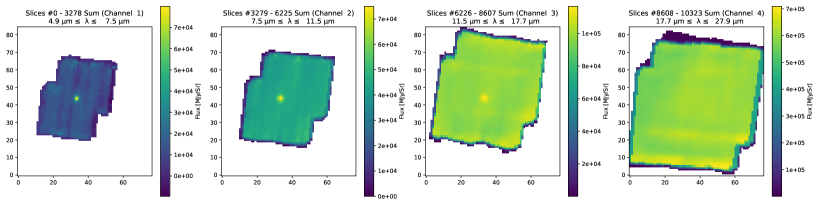
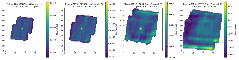
Figure 1: Top row: MIRI/MRS cube of SN 2022xkq before background subtraction, split into the four MIRI/MRS channels. The image shown for each channel is the collapsed sum of all its slices. Bottom row: MIRI/MRS cube of SN 2022xkq after background subtraction. We note that although the SN cannot be seen in the stacked Channel 4 cube, it is visible in specific wavelength slices, as can be seen from the spectra in Figure 2.

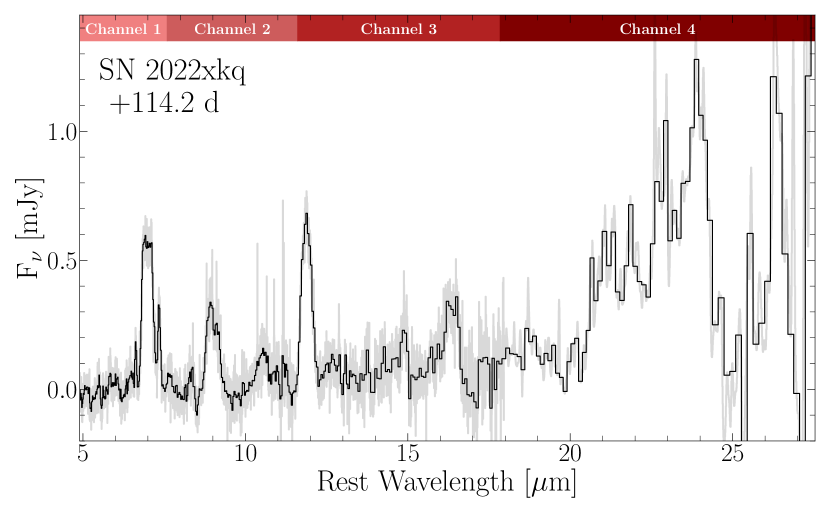
Figure 2: JWST MIRI/MRS observations of SN 2022xkq at $+114.2$ days relative to $B$-band maximum, corrected for Milky Way extinction. Raw data points are shown in grey, with the Spextractor (Burrow et al., 2020) smoothed spectrum in black. The channel labels at along the top axis are also corrected to the rest-frame of the SN.

The data were reduced using a custom-built pipeline designed to extract point source observations with a highly varying and/or complex backgrounds from MRS data cubes. This pipeline is discussed in detail in Appendix A of Shahbandeh et al. 2023 (in prep). In short, the pipeline creates a master background based upon 20 different positions in the data cube. This master background is then subtracted from the whole data cube before the aperture photometry is performed along the data cube, using the Extract1dStep in stage 3 of the JWST reduction pipeline. The reduction shown here utilized version 1.12.1 of the JWST Calibration pipeline (Bushouse et al., 2023) and Calibration Reference Data System files version 11.17.1. The resulting MIRI/MRS cube is shown in Figure 1 and the spectrum is shown in full in Figure 2. The raw data associated with this reduction can be found at 10.17909/kfvh-wb96 (catalog DOI:10.17909/kfvh-wb96). The extracted spectrum has been smoothed with spextractor (Burrow et al., 2020) channel-by-channel to properly account for the differences in resolution across the full MIRI/MRS wavelength coverage.

3 Line Identifications

To identify the lines present in our $+114.2$ day spectrum of SN 2022xkq, we are guided by lines previously identified in other MIR spectra of normal-luminosity SNe Ia, as well as using the full non-LTE radiation-hydrodynamic models of the under-luminous SN 2022xkq presented in § 5. The line identifications are presented by MIRI/MRS channel in Figure 3, with individual lines specified in Table 3. We only identify features strong enough to exceed a flux level of 5% of the maximum flux of the smoothed spectrum at $\lambda<20$ $\mu$m, or 10% of the maximum flux in the channel the feature is found, whichever is greater. Weaker features at or slightly exceeding the threshold level are considered tentative identifications.

At this phase, the ejecta is not yet fully nebular; meaning there is a combination of both permitted lines, forbidden emission, and an underlying continuum to the spectrum, creating a pseudo-photosphere (see § 5), seen previously in the analysis of both SNe 2005df and 2014J at similar epochs (Gerardy et al., 2007; Diamond et al., 2015; Telesco et al., 2015). This results in many of the features arising from a combination of blends as well as radiative transfer effects, making the identification of individual components difficult. Below we discuss clear feature detections, but note that many weak lines have no cross sections. Work to determine these missing cross-sections using the MRS spectra of SN 2021aefx in combination with detailed non-LTE simulations is in progress (Ashall et al. in prep).

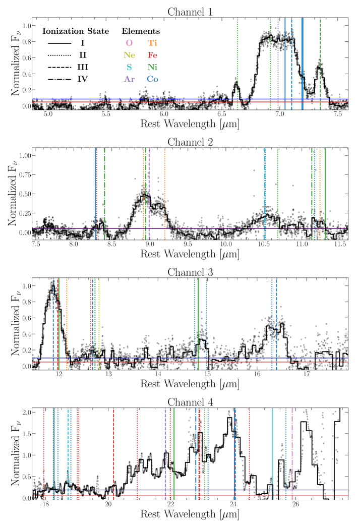
Figure 3: Spectrum of SN 2022xkq with line identifications based on known lines from previous MIR SNe Ia observations and models of under-luminous SN Ia models. The horizontal lines denote the two threshold values of 5% of the overall flux (red) and 10% of maximum flux in each individual channel (blue); the larger of which must be exceeded for a feature to have line identifications.

3.1 Channel 1 (4.9–7.65 $\mu$m)

Channel 1 is dominated by a large, complex, seemingly box-shaped profile near $\sim 7.0$ $\mu$m, with more isolated peaks on either side. These isolated peaks are easily identified as [Ni II] 6.636 $\mu$m, and [Ni III] 7.349 $\mu$m lines arising from stable ⁵⁸Ni present in the ejecta. Both peaks appear blue-shifted relative to their rest wavelengths and are further explored in § 4.

As seen in the top panel of Figure 3, the dominant box-like feature reveals several peaks. This feature is primarily due to the [Ar II] 6.985 $\mu$m line seen in other SNe Ia spectra, with additional weak peaks across the box-like profile matching [Ni II] 6.920 $\mu$m, [Co I] 7.045 $\mu$m, and [Co III] 7.103 $\mu$m lines. A shoulder on the red side of this feature likely arises from a blend of [Co I] 7.191 $\mu$m and 7.200 $\mu$m lines. The [Ni III] 7.349 $\mu$m line also shows a weak shoulder in its red wing, which is likely attributable to the quasi-continuum (Fesen et al., 2015; Hoeflich et al., 2023).

No other strong features are present in the channel. Hints of weak, broad features appear in the $\sim$5–6.5 $\mu$m region, but none are well-matched by known spectral lines. The broad feature spanning $\sim$5.8–6.1 $\mu$m may arise in part from a blend of [Ni I] 5.893 and [Ni II] 5.953 $\mu$m, lines, but it is unclear how much of the flux is due to the emission from forbidden Ni lines. As such, we leave this feature unidentified in both Figure 3 and Table 3.

3.2 Channel 2 (7.51–11.7 $\mu$m)

Similar to Channel 1, Channel 2 is also dominated by a single prominent feature, with additional weak features spread across the channel. The strongest feature is the blended feature near $9.0$ $\mu$m. This blend shows a strong blue peak at $\sim$8.9 $\mu$m, likely from [Ni IV] 8.945 $\mu$m with some contribution of [Ti II] 8.915 $\mu$m. This peak is blended with the central line of the feature, [Ar III] 8.991 $\mu$m. A secondary peak in the red at roughly $\sim$9.1 $\mu$m could be produced from [Ti II] 9.197 $\mu$m, however, due to the increased noise in this part of the feature, it may be more shoulder-like in appearance with stronger contributions from additional iron group elements and/or the quasi-continuum. Due to the combination of this blending and asymmetry in the feature the exact profile of the [Ar III] 8.991 $\mu$m is difficult to determine requiring detailed models (e.g. Penney & Hoeflich, 2014; Hoeflich et al., 2021), like in SN 2021aefx (Kwok et al., 2023a; DerKacy et al., 2023).

We tentatively identify some weaker features in Channel 2. The double-peaked feature from $\sim$8.2–8.4 $\mu$m is due to [Co I] 8.283 $\mu$m, [Fe II] 8.299 $\mu$m, and [Ni IV] 8.405 $\mu$m. A broad but weak blend is seen extending from roughly $\sim$10–11.4 $\mu$m, with contributions likely originating from [S IV] 10.511 $\mu$m, [Ti II] 10.511 $\mu$m, [Co II] 10.523 $\mu$m, and [N II] 10.682 $\mu$m. A narrower, but equally weak feature exists between $\sim$11.1–11.4 $\mu$m, potentially arising from [Ni IV] 11.130 $\mu$m, [Co II] 11.167 $\mu$m, [Ti II] 11.238 $\mu$m, and [Ni I] 11.307 $\mu$m lines.

Channel 2 terminates at roughly 11.7 $\mu$m, within the blue edge of the feature dominated by the [Co III] 11.888 $\mu$m resonance line. As the bulk of the feature is observed within Channel 3, we discuss the feature in the following section.

Table 3: Line Identifications

Line	$\lambda$ ($\mu$m)	Line	$\lambda$ ($\mu$m)	Line	$\lambda$ ($\mu$m)
Lines in Strong Features
[Ni II]	6.636	[Ni IV]†	8.945	[Co II]†	16.155
[Ni II]†	6.920	[Ar II]†	8.991	[Co II]†	16.299
[Ar II]†	6.985	[Ti II]†	9.197	[Co III]†	16.391
[Co I]†	7.045	[Co III]†	11.888	[Fe II]†	17.936
[Co III]†	7.103	[Fe III]†	11.978	[Ni II]†	18.241
[Co I]†	7.191	[Ni I]†	12.001	[Co I]†	18.265
[Co I]†	7.200	[Ni I]†	14.814	[Co II]†	18.390
[Ni III]	7.349	[Co II]†	14.977	[S III]†	18.713
[Ti II]†	8.915	[Co II]†	16.152	[Co II]†	18.804
Lines in Weak Features
[Co II]†	8.283	[Fe III]†	12.642	[Fe II]†	22.902
[Fe II]†	8.299	[Co III]†	12.681	[Fe III]†	22.925
[Ni II]†	8.405	[Ni II]†	12.729	[Ni II]†	23.086
[S IV]†	10.511	[Ne II]†	12.811	[Co II]†	23.196
[Ti II]†	10.511	[Co II]†	14.739	[Co IV]†	24.040
[Co II]†	10.523	[Co II]†	15.936	[Fe I]†	24.042
[Ni II]†	10.682	[Fe III]	20.167	[Co III]†	24.070
[Ni IV]†	11.130	[Fe II]†	20.928	[S I]	25.249
[Co II]†	11.167	[Ar III]†	21.829	[Co II]	25.689
[Ti II]†	11.238	[Fe II]†	20.986	[O IV]	25.890
[Ni I]†	11.307	[Ni I]†	22.106
[Ti II]†	12.159	[Co IV]†	22.800

Note. — ^†denotes line is part of a blended feature.

3.3 Channel 3 (11.55–18 $\mu$m)

Channel 3 begins in the blue wing of the [Co III] 11.888 $\mu$m blended feature. When examined as a whole, this feature is clearly dominated by [Co III] 11.888 $\mu$m, with the [Fe III] 11.978 $\mu$m and [Ni I] 12.001 $\mu$m lines making weaker contributions to the red shoulder, as previously seen in SN 2021aefx (DerKacy et al., 2023), with additional weak contributions due to [Ti II] 12.159 $\mu$m. Also similar to SN 2021aefx, a broad, multi-peaked blend of weak features spanning $\sim$12.4–13 $\mu$m potentially results from [Fe II] 12.642 $\mu$m, [Co III] 12.681 $\mu$m, [Ni II] 12.729 $\mu$m, and [Ne II] 12.811 $\mu$m lines (DerKacy et al., 2023; Blondin et al., 2023).

Beyond $\sim$14 $\mu$m, hints of strong features are seen between 14.6–15 $\mu$m and 15.6–16.8 $\mu$m. The former is likely the result of a complex of [Co II] 14.739 $\mu$m, [Ni I] 14.814 $\mu$m, and [Co II] 14.977 $\mu$m. In the latter, we identify the primary lines contributing to the main peak as [Co II] 16.152 $\mu$m, 16.155 $\mu$m, and 16.299 $\mu$m, and [Co III] 16.391 $\mu$m. These are the first line identifications in this wavelength range for a SN Ia.

In much of the remaining parts of the channel, small peaks are seen at low significance and remain unidentified. Many of these peaks are expected to be contributions from weak iron-group lines with no measured cross-sections. This is important for the astro-atomic physics community to address, with cross-validation between astronomical and atomic physics methods.

3.4 Channel 4 (17.7–27.9 $\mu$m)

We see a clear point source present in the SHORT sub-band of Channel 4 (17.70–20.95 $\mu$m). Between $\sim$18–19 $\mu$m, a broad, possibly multi-peaked feature is discernible, arising from [Fe II] 17.936 $\mu$m, [Ni II] 18.241 $\mu$m, [Co I] 18.265 $\mu$m, [Co II] 18.390 $\mu$m, [S III] 18.713 $\mu$m, [Co II] 18.804 $\mu$m, [Fe II] 19.007 $\mu$m, and [Fe II] 19.056 $\mu$m lines. In the MEDIUM and LONG sub-bands, the background becomes much more variable possibly due to the decreased sensitivity in Channel 4. This results in a likely under-subtraction which appears as a growing continuum under the strong peaks. This continuum should not be interpreted as due to any physical process. Regardless of this we see a clear point source in specific wavelength slices. Additionally, this continuum pushes the entire flux above the 10% strong line threshold, and to account for this uncertainty, we only tentatively identify lines associated with clear peaks and group them with the weak detections from Channels 1–3. Lines roughly corresponding to strong and/or broad peaks in the complex blends of the MEDIUM and LONG sub-bands include: [Fe III] 20.167 $\mu$m, [Fe II] 20.928 $\mu$m, [Ar III] 21.829 $\mu$m, [Fe II] 20.986 $\mu$m, [Ni I] 22.106 $\mu$m, a possibly blue-shifted line of [Co IV] 22.800 $\mu$m, [Fe II] 22.902 $\mu$m, [Fe III] 22.925 $\mu$m, [Ni II] 23.086 $\mu$m, [Co II] 23.196 $\mu$m, [Co IV] 24.040 $\mu$m, [Fe I] 24.042 $\mu$m, and [Co III] 24.070 $\mu$m. Relatively isolated peaks associated with [S I] 25.249 $\mu$m, [Co II] 25.689 $\mu$m, and [O IV] 25.890 $\mu$m are also tentatively identified. As in Channel 3, many of the unidentified peaks likely correspond to weak iron-group lines lacking measured cross-sections. Therefore, in order to obtain more information about which lines may be expected at $\lambda\gtrsim 21$ $\mu$m and at what fluxes in under-luminous SNe Ia, we turn to model synthetic spectra in § 5.

4 Characterization of under-luminous SN Ia

Having identified the strong lines present in the MIR features of SN 2022xkq, we now attempt to measure the physical properties of these lines through spectral fitting. These fits allow us to estimate the central location and widths of the lines. However, due to line blending, the complex physics of line formation at these epochs (see again § 3 and later, § 5), and the unknown strengths of many weak lines that produce the observed features in the spectrum, the resulting fits to most of the strong features in the spectrum are arbitrary with little physical meaning. By this we mean that the peak of the fit, or its individual sub-components, cannot be identified with any particular transition and thus it cannot directly probe the ejecta velocity.

Instead, we focus on fitting only those features that are relatively well isolated and result from lines with known cross-sections, such as the [Ni II] 6.636 $\mu$m, [Ni III] 7.349 $\mu$m, and [Co III] 11.888 $\mu$m lines. For analysis of the more complex features, we take a data-only approach to estimating parameters from the features as a whole. The results of these measurements and their implications are discussed below.

4.1 Velocities of Isolated Lines

Among the strong features present in the observed spectrum of SN 2022xkq, only three are isolated enough with minimal blending to be fit with simple analytic functions. These features are those dominated by the [Ni II] 6.636 $\mu$m, [Ni III] 7.349 $\mu$m, and [Co III] 11.888 $\mu$m lines. In each case, the fits were performed using the modified trust-region Levenberg-Marquardt algorithm found in the scipy.odr package. Each spectral region was fit with a Gaussian function with amplitude, mean, and standard deviation taken as free parameters. In order to better estimate the fit uncertainties, a Monte Carlo (MC) method was used to re-sample the spectrum (i.e. bootstrapping) and repeat the fit 500 times. The errors of the MC sample are then added to the known uncertainties of the data, such as spectral resolution, in quadrature to obtain the values presented below.

4.1.1 Stable Ni Lines

In all previously published MIR spectra of SNe Ia with the corresponding wavelength coverage, the [Ni II] 6.636 $\mu$m line has either been not detected (Gerardy et al., 2007), or identified as part of a blended feature (Kwok et al., 2023a; DerKacy et al., 2023; Kwok et al., 2023b). In our MRS spectrum of SN 2022xkq, we see this feature as isolated and unblended — suggesting it should be representative of the stable Ni distribution within the core of the ejecta. Given the shape of the line profile, it is assumed that the emission is coming from a region of the ejecta which has already reached the nebular state and can be modeled by a Gaussian function. However, it should be noted that fitting emission features with Gaussian profiles makes implicit assumptions about the nature of the line formation and spectral features (see § 5), the underlying chemical distribution of ions within the ejecta, and should therefore be interpreted with caution. The resulting fit is shown in Figure 4, revealing a shift in the line center of $-460\pm 110$ km s^-1, and a full-width at half-maximum (FWHM) of $2460\pm 110$ km s^-1.

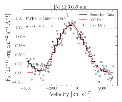
Figure 4: Single Gaussian MC fit to the [Ni II] 6.636 $\mu$m line. The best-fit parameters as determined from the MC results are: $\mu=-460\pm 2$ km s^-1 and FWHM $=2460\pm 5$ km s^-1. The resolution error of 110 km s^-1 dominates over both the uncertainties in the fit and in the wavelength calibration ($\sim$6 km s^-1; Argyriou et al., 2023).

Similarly, the [Ni III] 7.349 $\mu$m feature in SN 2022xkq is more isolated and unblended than in previous MIR observations of SNe Ia. However, compared to the [Ni II] 6.636 $\mu$m feature, fitting the [Ni III] feature requires more careful treatment. There is a significant contribution to the blue wing of the profile either from the continuum or an unknown weak line, and a weak shoulder in the red wing also due to unidentified lines. Neither wing component matches known nebular lines near these wavelengths.

Initial attempts to fit the profile despite these complications yield a fit which captures the width of the profile, but is unable to accurately measure the peak of the flux. Attempts to simultaneously account for potential contributions from the continuum and weak blending similarly capture the width of the feature, but are also unable to reproduce the correct location of the peak flux, and are strongly dependent on the choice of initial parameters defining the continuum.

Penney & Hoeflich (2014) have noted that prior to the ejecta becoming optically thin through to the center, the locations of the peak fluxes will appear blue shifted relative to the true line center due to blocking of the red half of the line profile by the continuum, and that these effects are best measured after subtracting the continuum flux separately. After subtracting the continuum separately, the profile appears noticeably less Gaussian and requires at least a two Gaussian fit. The result of this fit captures the peak of the flux and width of the feature well, however the assumed [Ni III] component is not the dominant line in the feature. Additionally, the strong component is not near the correct location to fit the weak blending in the wings from the possible [Co I] lines. As there are no nearby lines resulting from ions commonly found in models of under-luminous SN Ia, we regard the presence of an unidentified, strong line as unlikely.

Instead, we estimate the shift in the peak flux and the FWHM from a sample of 1000 bootstrapped re-sampled MC realizations of the spectra, assuming the flux errors are normally distributed. We find that the peak flux is shifted by $-160\pm 140$ km s^-1, with the FWHM of the feature measuring 3800 km s^-1. The results of this work are shown in Figure 5, and highlight the complexity of fitting even seemingly isolated and weakly blended features, and the effects of the photosphere present even during this late phase. Furthermore, Gaussian fits to complex features need to be interpreted with caution, as they fail to capture the physics of the line formation of these features, even at late times.

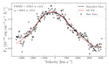
(a) Single Gaussian MC fit

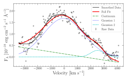
(b) Simultaneous multi-component fit

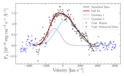
(c) Continuum-subtracted MC multi-Gaussian fit

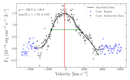
(d) Continuum-subtracted data derived values

Figure 5: Fits to the [Ni III] 7.349 $\mu$m feature. Panel (a) shows the results of a single Gaussian fit similar to Figure 4. Panel (b) simultaneously fits the continuum component and multiple Gaussians, illustrating the non-Gaussianity of the feature. Panel (c) fits multiple Gaussian components after independently fitting and subtracting the continuum. Panel (d) shows the data derived values as measured from the continuum subtracted line profile.

4.1.2 [Co III] 11.888 $\mu$m Feature

Resonance lines such as [Co III] 11.888 $\mu$m are important tracers of the amount and distribution of ions in the SN ejecta, since most of the de-excitation and recombination of each species will pass through their resonance transitions. Due to the decay chain of ⁵⁶Ni $\rightarrow$ ⁵⁶Co $\rightarrow$ ⁵⁶Fe which powers the emission in SNe Ia, the [Co III] 11.888 $\mu$m feature serves as a late-time tracer of the initial ⁵⁶Ni distribution, which is located below the photosphere at early times. Previous low resolution observations of the features dominated by [Co III] 11.888 $\mu$m have found that the line profiles are well-captured by a single Gaussian fit; however, spectral modeling reveals that up to $\sim$10 percent of the flux in the feature may result from weak blending with [Fe III] 11.978 $\mu$m and [Ni I] 12.001 $\mu$m lines in the red wing of the profile (Telesco et al., 2015; Kwok et al., 2023a; DerKacy et al., 2023).

In SN 2022xkq, the effects of the blending are clearly seen as a series of shoulders in the red wing of the profile in Figure 6 that are not present in the blue wing of the feature. However, much like the previous lower-resolution observations, the velocity shift, peak flux, and width of the feature are well-represented by a single Gaussian fit, with the line center shifted by $-170\pm 110$ km s^-1 and a FWHM of $8810\pm 110$ km s^-1. As in the fits to the [Ni III] 6.636 $\mu$m line, the resolution error dominates over the statistical error of the fit. Comparisons between these fits in SN 2022xkq and the sample of other observed normal-luminosity SNe Ia are explored in further detail in § 4.2. This highlights the need to approach Gaussian fits with caution, as the effects of blending are even stronger in the [Co III] 11.888 feature than in the [Ni III] 7.349 feature, despite the fact that a single Gaussian fit is sufficient to approximate the blended feature in this instance.

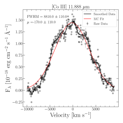
Figure 6: Same as Figure 4 but for the [Co III] 11.888 $\mu$m-dominated feature. The best fit parameters determined from the MC ensemble are: $\mu=-170\pm 5$ km s^-1 and FWHM $=8810\pm 5$ km s^-1. As before, the resolution error of $\pm 110$ km s^-1 dominates over the fit and wavelength calibration errors.

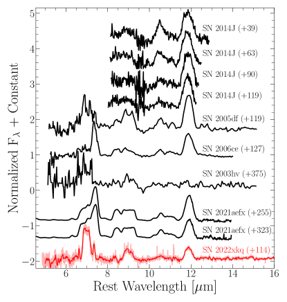
Figure 7: The published sample of normal-luminosity SNe Ia MIR spectral observations, including SNe 2003hv, 2005df (Gerardy et al., 2007), 2006ce (Kwok et al., 2023a), 2014J (Telesco et al., 2015), and 2021aefx (Kwok et al., 2023a; DerKacy et al., 2023). Epochs relative to $B$-band maximum are shown for each spectrum. For SN 2022xkq, a smoothed spectrum is shown in the foreground while the raw data is shown in the background. All spectra have been corrected for MW extinction.

Table 4: Properties of SNe Ia with MIR Spectra at $\sim$120 Days

Parameter	SN 2005df	SN 2006ce	SN 2014J	SN 2022xkq
Epoch (days)	119	127	119	114.2
MB,peak (mag)	$-19.27\pm 0.31$	$\cdots$	$-19.19\pm 0.10$	$-18.01\pm 0.15$
$\Delta{\rm m_{15}(B)}$ (mag)	1.12	$\cdots$	$1.12\pm 0.02$	$1.65\pm 0.03$
sBV	0.95	$\cdots$	0.95	0.63
d (Mpc)	$19.8\pm 2.8$	$19.6\pm 2.87$	$3.4\pm 0.1$	$31.0\pm 2.0$

Note. — No optical photometry of SN 2006ce is publicly available.

References. — SN 2005df: Takáts et al. (2015); Krisciunas et al. (2017), SN 2006ce: Kwok et al. (2023a); NED, SN 2014J: Marion et al. (2015), SN 2022xkq: Pearson et al. (2023), This work.

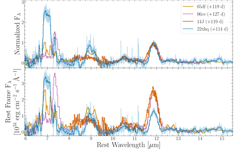
Figure 8: Comparison of SNe Ia spectra observed $\sim$120 days after maximum light in the MIR. The top panel shows flux values normalized to the peak of the [Co III] 11.888 $\mu$m features, while the bottom panel shows the fluxes corrected to the SN rest frame based on the estimated distances in § 4.1.2. In SN 2022xkq, the singly ionized features (e.g. [Ni II] 6.636 $\mu$m and [Ar II] 6.985 $\mu$m) are stronger relative to their doubly ionized counterparts ([Ni III] 7.349 $\mu$m and [Ar III] 8.991 $\mu$m) as is expected in an under-luminous SN Ia.

4.2 Under-luminous vs. Normal-luminosity SNe Ia MIR Spectra

4.2.1 Qualitative Comparisons

The published MIR sample of normal-luminosity SNe Ia are compared to our spectrum of SN 2022xkq in Figure 7. Four objects in the sample (SNe 2005df, 2006ce, 2014J, and 2022xkq) have MIR spectra taken roughly 120 days after $B$-band maximum light. These objects are directly compared in Figure 8.

The most prominent difference between the MIR spectrum of SN 2022xkq and the sample of normal-luminosity objects is the strength of the [Ar II] feature near 7 $\mu$m relative to the [Ar III] feature at $\sim$9 $\mu$m. These features are known to vary based on the geometry of the Ar distribution and viewing angle of the SN (Gerardy et al., 2007; DerKacy et al., 2023), although distinguishing these effects from continuum effects in spectra taken before the ejecta become fully nebular is much more difficult. Yet, when comparing the line identifications in SN 2022xkq to those of the rest of the sample, we find the elements that dominate these features are similar, and produce prominent features in the same wavelength regions. The differences in the [Ar] lines are explored further in both § 4.2.2 and § 5.

Both the under-luminous SN 2022xkq and the sample of normal-luminosity objects display weak, blended, broad features in the region between $\sim$10–11.5 $\mu$m (Figure 8). When compared to previous observations normalized to the peak of the [Co III] 11.888 $\mu$m resonance line, the relative flux in the features are similar. Spectra taken roughly 130 days after explosion have tentative identifications of [S IV] in combination with iron group elements (e.g. Fe, Co, and Ni) while the later spectra of SN 2021aefx only show the iron-group lines (Kwok et al., 2023a; DerKacy et al., 2023). The low spectral resolutions of previous observations make further direct comparisons difficult.

As expected, due to the under-luminous nature of SN 2022xkq, the peak flux of the [Co III] 11.888 $\mu$m resonance line is significantly weaker than in the other objects in the sample at similar epochs, all of which are normal-luminosity SN Ia (see the bottom panel of Figure 8). As a resonance line, the [Co III] 11.888 $\mu$m line directly traces the radioactive decay of the ⁵⁶Ni produced in the explosion through the ⁵⁶Ni $\rightarrow$⁵⁶Co $\rightarrow$⁵⁶Fe decay chain. The [Co III] line is also noticeably narrower than the other normal-luminosity SNe Ia in the sample, consistent with measurements of the [Co III] 5890 Å in the optical (Graham et al., 2022). This behavior is also expected for under-luminous SNe Ia, as nuclear burning occurs under lower density compared to normal SNe Ia resulting in lower ⁵⁶Ni production and a shift of nuclear burning products towards the inner, slower expanding layers. Moreover, more quasi-statistical equilibrium (QSE) elements are formed at the expense of nuclear statistical equilibrium (NSE) elements leading to increasing [Ar II/III] emission and narrower lines of all QSE and NSE elements (Höflich et al., 2002a; Ashall et al., 2018; Mazzali et al., 2020). The differences in these [Co III] lines are quantified in § 4.2.3.

4.2.2 Ar Lines

Figure 9 shows the region of the two prominent argon features, [Ar II] 6.985 $\mu m$ and [Ar III] 8.991 $\mu m$, in SN 2022xkq compared to the same features in the subset of normal-luminosity SNe Ia spectra taken near 120 days after maximum light. For the normal-luminosity SNe Ia, it is difficult to ascertain the exact extent of the emission in velocity space due to a combination of low resolution and low S/N in the individual observations. However, for SN 2022xkq it is clear that the wings of the emissions extend to $\sim$10,000 km s^-1 in both argon dominated features. The ionization balance of SN 2022xkq is noticeably different than that of the other objects. In SN 2022xkq, the bulk of the argon is singly ionized, resulting in an average ratio of the peak flux of $\sim$2 between the [Ar II] and [Ar III] dominated features. In the normal-luminosity objects observed at similar epochs, this ratio is $\sim$1. Furthermore, the total integrated flux in the Ar regions relative to the peak of the [Co III] is higher in SN 2022xkq, demonstrating that there is a larger argon abundance in the ejecta relative to the ⁵⁶Ni mass, as expected for an under-luminous SN Ia (Ashall et al., 2018).

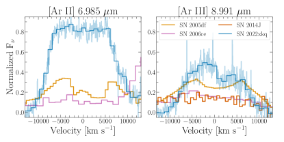
Figure 9: Comparison of Ar line profiles between SN 2022xkq and other normal-luminosity SNe Ia roughly 120 days after $B$-band max. As expected, the overall fluxes in the [Ar]-dominated features are larger in SN 2022xkq than in the normal-luminosity objects, while the increased strength of the [Ar II] feature relative to the [Ar III] feature in SN 2022xkq indicates that the ionization balance in the ejecta favors Ar II over Ar III (Gerardy et al., 2007; Ashall et al., 2018; Mazzali et al., 2020).

4.2.3 [Co III] 11.888 $\mu$m Profiles

Figure 10 shows the comparison of the [Co III] 11.888 $\mu$m features across the sample of MIR spectra taken $\sim$120 days after $B$-max. Compared to the lower-resolution observations with Spitzer (SNe 2005df, 2006ce) and CanariCam (SN 2014J) that smooth out much of the blending and continuum effects, the profile of SN 2022xkq is decidedly non-Gaussian. The blending effects primarily impact the red wings of the profile, with all four SNe showing similar full widths at zero-intensity (FWZI). These effects are not prominent in the blue wing, where the FWZI of SN 2022xkq at $\sim$7,500 km s^-1 is narrower than those of the normal-luminosity objects ($\gtrsim$10,000 km s^-1).

As a consequence of the [Co III] 11.888 $\mu$m resonance line being formed by the radioactive ⁵⁶Co in the ejecta, it serves as a direct tracer of the original distribution of ⁵⁶Ni in the explosion. As such, the width of the feature is characteristic of the burning conditions of the NSE region. As previously discussed above for under-luminous SNe Ia, burning to ⁵⁶Ni occurs more centrally in the ejecta, which has the effect of producing a narrower [Co III] 11.888 $\mu$m feature.

Figure 11 shows the FWHM of this [Co III] 11.888 $\mu$m feature as a function of light curve shape, $\Delta{\rm m_{15}(B)}$. We see a rough trend between light curve shape and width of the [Co III] 11.888 $\mu$m feature, where broader, more luminous SNe Ia have larger values of FWHM compared to the under-luminous SN 2022xkq. As the sample of MIR spectra of SNe Ia increases, this figure can be populated with various types of SNe Ia to understand how closely the [Co III] 11.888 $\mu$m feature traces the luminosity of the SNe, allowing us to see how closely this plot follows the luminosity-width relation (Phillips, 1993). A similar trend has been found through spectral modeling of the optical data (Mazzali et al., 1998, 2007), as well as in the [Co III] 5890 Å line in optical nebular spectra (Graham et al., 2022). While both the optical and MIR [Co III] lines are resonance lines, it is important to test this relation with the MIR line that is from a very low lying state from which the resonance transition is the only downward transition out of this low lying state. The more energetic upper state of the [Co III] 5890 Å transition in addition to decaying to the ground state, also decays to the upper state of the MIR line. The optical line from this transition at 6190 Å is not a prominent feature in the spectra shown by Graham et al. (2022), nor are other nearby [Co III] resonance lines. There is also disagreement in the literature about whether the feature associated with [Co III] 5980 Å is due (in part) to Na I D (Kuchner et al., 1994; Mazzali et al., 1997; Dessart et al., 2014).

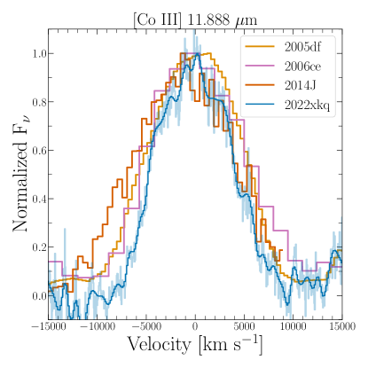
Figure 10: Same as Figure 9, but instead comparing the [Co III] 11.888 $\mu$m dominated features. The unblended blue wings of the profile reveal SN 2022xkq has a much narrower distribution of ⁵⁶Co relative to the normal-luminosity objects.

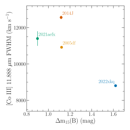
Figure 11: [Co III] 11.888 $\mu$m FWHM versus $\Delta{\rm m_{15}(B)}$ for SNe Ia with detected [Co III] emission and well-characterized light curves. We include the value from SN 2021aefx obtained at $\sim+323$ days from the explosion (DerKacy et al., 2023), but note that this value may be uncertain due to the different physical regime in which the epoch is measured and potential line blending.

5 Modeling

We compare SN 2022xkq to new simulations of off-center M_Ch explosion models, with parameters based upon the spherical models of the Model 16-series of Hoeflich et al. (2017). The early light curve properties and maximum light luminosity of the models are very similar to that of SN 2022xkq. No further fine-tuning of the basic parameters have been done, nor is it is necessary in light of uncertainties in distance and reddening. In order to move beyond profile fits, the synthetic spectra are modeled by detailed non-LTE radiation-hydrodynamic simulations, which link the observations to the underlying physics identify and quantify the contribution of specific transitions to observed spectral features. The observed features are dominated by a combination of emission lines, a quasi-continuum of allowed and forbidden lines in an envelope with varying element abundances, and strong non-LTE effects. We choose our best-fit model by comparing line profiles and line-ratios of noble gases like Ar and of electron capture elements such as Ni.

Table 5: Model parameters and light curve parameters for various $\rho_{c}$.

Parameter	Value	Value	Value	Value
$\rho_{c}[\times 10^{9}$ g cm-3 ]	0.5	1.0	2.0	4.0
Mej (M⊙)	$\sim$1.37	$\sim$1.37	$\sim$1.37	$\sim$1.37
Mtr (M⊙)	0.33	0.34	0.34	0.36
B(WD, turbulent) (G)	$10^{6}$	$10^{6}$	$10^{6}$	$10^{6}$
M(B/V) (mag)	-18.43/-18.57	-18.29/-18.46	-18.22/-18.37	-17.98/-18.06
$\Delta$m${}_{15}(B/V)$ (mag)	1.61/1.15	1.65/1.16	1.67/1.18	1.42/1.02
B-V (Vmax) (mag)	0.150	0.152	0.152	0.158

Note. — The DDT is unlikely to occur between 0.3–0.5 $M_{\odot}$ because overlapping of the Ca-rich layers with the bulge of the ⁵⁶Ni would lead to a narrow [Ca II] doublet. The amount of mass burned during the deflagration M_tr includes both ⁵⁶Ni and EC elements.

The simulations are parameterized explosion models, where we use the spherical delayed-detonation scenario to constrain the global parameters of the explosion. Fine-tuning these models is not necessary to achieve the goals of this study, as we focus on spectra rather than high-precision photometry. The reference model (Figure 12) originates from a C/O WD with a main-sequence progenitor mass of $5$ M_⊙, solar metallicity, and a central density $\rho_{c}=2.0\times 10^{9}$ g cm^-3. The model produces $\sim$0.324 M_⊙ of ⁵⁶Ni. The resulting light curves have a peak brightness of $M(B)=-18.22$ mag and $M(V)=-18.37$ mag and light curve decline rates of $\Delta{\rm m_{15}(B)}$ $=1.67$ mag and $\Delta{\rm m_{15}(V)}$ $=1.18$ mag. These can be compared to $M(B)=-18.1\pm 0.15$ mag, and $\Delta{\rm m_{15}(B)}$ $=1.65\pm 0.03$ mag obtained from the early time light curve (Pearson et al., 2023). The inferred absolute brightness at maximum light depends sensitively on the reddening, the distance modulus, and their uncertainties. Pearson et al. (2023) estimated a ⁵⁶Ni-mass of $0.22\pm 0.03$ M_⊙ compared to the $0.34$ M_⊙ we obtain using nebular MIR spectra. Derived ⁵⁶Ni masses are uncertain, in particular for under-luminous SNe Ia because the Q- or $\alpha$- value in Arnett’s law varies from 0.8–1.6 over a small brightness range and similar differences occur among various methods (Höflich et al., 2002a; Stritzinger et al., 2006; Hoeflich et al., 2017). The value of the ⁵⁶Ni mass obtained here is consistent with that of Pearson et al. (2023) within the errors.

Our value of $\rho_{c}$ is chosen based upon the presence of stable Ni lines and to match the ionization balance in the observed MIR spectrum (see Figure 3 and § 5.2.1). Burning starts as a deflagration front near the center and transitions to a detonation (Khokhlov, 1991). The DDT is triggered by increasing the rate of burning by the Zeldovich-mechanism (Zel’dovich, 1940; von Neumann, 1942; Döring, 1943), that is, the mixing of burned and unburned material. Various mechanisms have been suggested to initiate the DDT transition, ranging from mixing by turbulence, shear flows at chemical boundaries, and differential rotation in the WD. Moreover, the mixing may depend on the conditions during the thermonuclear runaway (Khokhlov et al., 1997a; Livne, 1999; Yoon et al., 2004; Bell et al., 2004; Höflich, 2006; Hristov et al., 2018; Charignon & Chièze, 2013; Poludnenko et al., 2019; Brooker et al., 2021). Although the recently suggested mechanism of turbulent-driven DDT in the distributed regime of burning (Oran, 2011; Poludnenko et al., 2019) is consistent with the amount of deflagration burning in our parameterized models (Höflich et al., 2002a; Hoeflich et al., 2023), other DDT mechanisms may be realized. We evaluate constraints from the observations of SN 2022xkq, treating the location of the DDT as a free parameter.

In our simulations, the deflagration–detonation transition is triggered ‘by hand’ when $\sim$0.34 M_⊙ of the material has been burned by the deflagration front and is induced by the mixing of unburned fuel and hot ashes (Khokhlov, 1991). Our simulations take into account magnetic fields for the positrons. However, at 130 days, the mean free path of positrons is small even for small initial magnetic fields (Penney & Hoeflich, 2014). We assume $B=10^{6}$ G based upon our prior modeling of light curves and late-time nebular spectra (Diamond et al., 2015; Hristov et al., 2021). We have examined models where $\rho_{c}$ was varied from $0.5-4.0\times 10^{9}$ g cm^-3 in order to study the effect of the WD central density on the MIR spectra and conclude that $\rho_{c}=2.0\times 10^{9}$ g cm^-3 best reproduces the observations. The flux changes by $\sim 15$% between models with our fiducial value and those with $\rho_{c}=4\times 10^{9}$ g cm^-3, because the photosphere masks the appearance of very neutron-rich isotopes. However, lower central densities radically change the spectra.

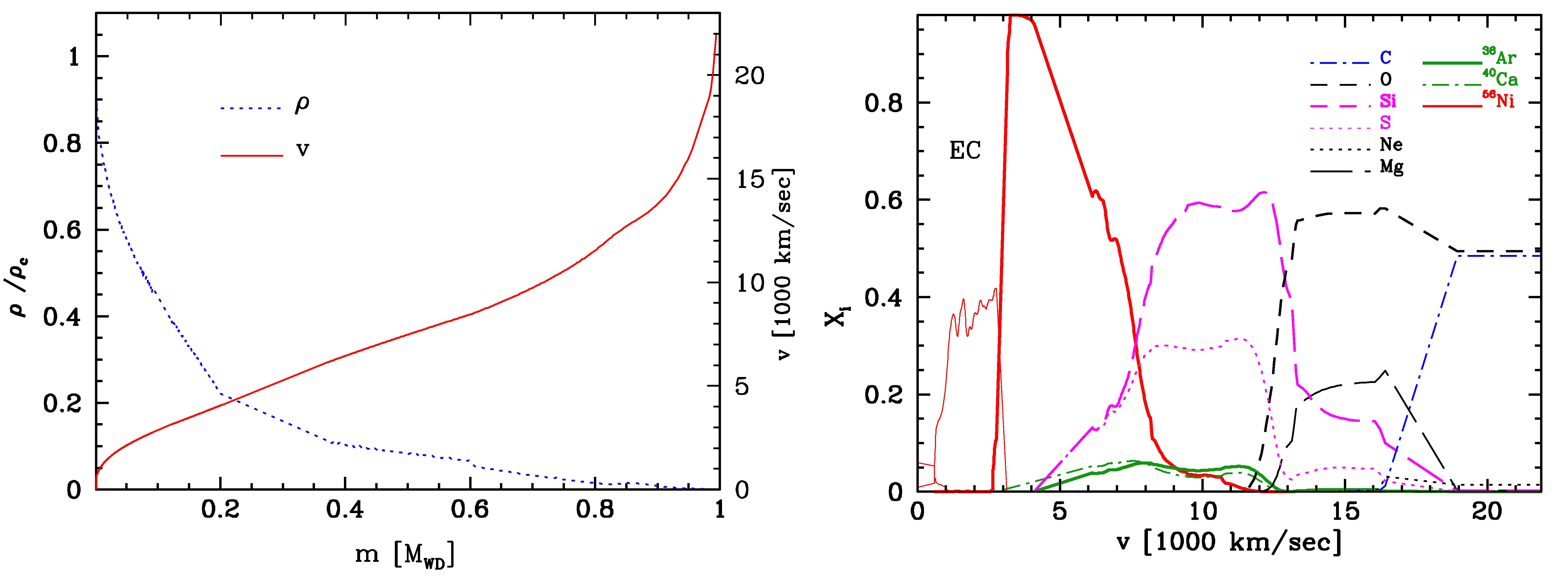
Figure 12: Density and velocity structure as a function of mass coordinate (left) and distribution of elements for our reference under-luminous models with $\rho_{c}=2\times 10^{9}$ g cm^-3. Note that M_DDT was chosen to be 0.2 M_⊙. For the influence of $\rho_{c}$ on the size electron capture core, see Diamond et al. (2015).

Following the central carbon ignition and the propagation of the deflagration front, the deflagration transitions to a detonation. Rather than assuming that the DDT occurs in a spherical shell, it is assumed to begin as an off-center point as described by Livne & Arnett (1995) and in our previous work (Penney & Hoeflich, 2014; Fesen et al., 2015; Hoeflich et al., 2021; DerKacy et al., 2023; Hoeflich et al., 2023). The effective spectral resolution is $R\approx 300-600$ (Hoeflich et al., 2021). We constructed models where the off-center location for the delayed-detonation transition occurred at M_DDT,off of 0, 0.2, 0.5, and 0.9 M_⊙. For computational expediency,only the model with 0.2 M_⊙ has been fully converged with complex model atoms. Note that we use an off-center DDT in a single spot because it does not produce a refraction wave. Based on the discussion in Hoeflich et al. (2021), the almost flat top of the [Ar II] 6.985 $\mu$m feature suggests that SN 2022xkq is seen at a low inclination angle ($\theta$) with $|\theta|\lesssim 20-30^{\circ}$. The absence of a narrow ($<1000$ km s^-1 FWHM) [Ca II] $\lambda\lambda 7293,7326$ Å doublet in SN 2022xkq (Pearson et al., 2023) excludes that the DDT occurs close to the inner edge of the ⁵⁶Ni region, justifying a M${}_{\rm DDT}\approx 0.2$ M_⊙., or less. This is in contrast with our models for SN 2020qxp where the large overlap between Ca-rich region and NSE region results in a strong and narrow [Ca II] feature appearing $\sim 100$ days after the explosion (see the inset of Fig. 4 in Hoeflich et al., 2021), regardless of the observation angle. Theoretically, a central DDT cannot be excluded because unburned material could be dragged down during the deflagration phase. However, the observed narrow ⁵⁸Ni features exclude a central DDT. The DDT is triggered by increasing the rate of burning by the Zeldovich-mechanism (Zel’dovich, 1940; von Neumann, 1942; Döring, 1943). At the time of the DDT, the expansion of the inner electron capture region is subsonic (see, for example, Figs. 9–10 in Hoeflich, 2017). Thus, with an increased rate of burning and energy production the buoyancy will mix the electron capture elements out to higher velocity, inconsistent with the observed narrow ⁵⁸Ni lines. For the best-fitting model (Figure 12), we used an off-center DDT with M${}_{\text{DDT,off}}=0.2$ M_⊙ because we have no strong evidence for asymmetry from the line profiles, either because the observing angle is close to the equator or because the DDT is well inside of the Ca/Ar region. Stronger constraints would require later time observations in the optical to MIR. Nonetheless, off-center DDTs have been used to avoid the artifact of low density burning due to the strong refraction wave evident in spherical simulations (Khokhlov et al., 1993; Hoeflich & Khokhlov, 1996).

The non-LTE atomic models and the radiation transport used in this work were discussed in Hoeflich et al. (2021). Detailed atomic models are used for the ionization stages I-IV for C, O, Ne, Mg, Si, S, Cl, Ar, Ca, Sc, Ti, V, Cr, Mn, Fe, Co, Ni. As before, the atomic models and line lists are based on the database for bound-bound ($\approx$ 40,000,000 allowed and forbidden) transitions of van Hoof (2018) supplemented by additional forbidden lines (Diamond et al., 2015), and lifetimes based on the analysis by our non-LTE models of SN 2021aefx (C. Ashall et al., in prep).

5.1 Model structure

The basic model parameters and light curve observables are given in Table 5. The angle averaged structure of the best fitting model is shown in Figure 12. As expected for ‘classical’ delayed detonation models, the density and velocity distributions are smooth (e.g without a shell) because the WD becomes unbound during the deflagration phase, in contrast to pulsating DD or pure deflagration models (Nomoto et al., 1984; Hoflich et al., 1995; Niemeyer & Woosley, 1997; Bravo et al., 2009; Hoeflich et al., 2017). Within the M_Ch scenario a low luminosity/low ⁵⁶Ni mass is produced by an increased mass of deflagration burning, which leads to a larger pre-expansion of the WD and lower density burning. Our model for SN 2022xkq falls into the $\Delta$m${}_{15}(B/V)$ regime of rapidly dropping opacities soon after maximum light, a regime of fast declining peak luminosity within a relatively narrow range of $\Delta$m${}_{15}(B/V)$ (Höflich et al., 2002a). This is similar to SN 1991bg-like objects (as indicated by the [Ti II] lines) and slightly more luminous than SN 2005ke or SN 2016hnk (Patat et al., 2012; Galbany et al., 2019). As a result, the models show unburned C/O, and products of explosive O-burning, and incomplete Si-burning layers down to $\approx$ 16,000, 12,000 and 5000 km s^-1, respectively. For M_Ch models of under-luminous SNe Ia, the element production is shifted toward partial burned fuel corresponding to: $\sim$0.27–0.35 M_⊙ of M(⁵⁶Ni), $\sim$0.65 M_⊙ of intermediate mass elements (Si and S), and $\sim$0.1 M_⊙ of unburned carbon (Höflich et al., 2002a). In models of normal-luminosity SNe Ia, these values are 0.55–0.65 M_⊙, 0.2 M_⊙, and $1-2\times 10^{-2}$ M_⊙, respectively (Höflich et al., 2002a). In our reference model, the layers expanding interior to $\approx 3000$ km s^-1 are dominated by electron capture elements, mostly ⁵⁴Fe, ⁵⁷Co and ⁵⁸Ni.

Figure 13: Same as the right panel from Figure 12 but angle-averaged ionization levels I-IV of Fe and Co as representative of iron-group elements, specific energy input by $\gamma$-rays and non-thermal leptons normalized to its maximum, and temperature T as a function of expansion velocity. Note that the overall ionization structure is rather insensitive to $\rho_{c}$ because the shift in the balance is dominated by the recombination rate and, thus, the density. $E_{\gamma}$ is dominated by $\gamma$-rays rather than positrons which only is loosely correlated with the ⁵⁶Ni distribution. Namely, $E_{\gamma}$ escape the outer layers and we have significant heating in the core resulting in overall peaked line profiles of the iron group elements (see below and Figure 15).

The ionization structures at day 130 are shown in Figure 13. Overall, when compared to normal-luminosity SNe Ia (e.g., Wilk et al., 2020), the global ionization balances are shifted towards lower ionization states, as has also been shown for other under-luminous SNe Ia, (Hoeflich et al., 2021). All the non-iron-group elements (e.g. C, O, Mg, Si, S, Ca) are dominated by singly ionized features, with significant contribution from neutral ions. For iron group elements, doubly ionized species dominate in the ⁵⁶Ni region, but the equilibrium is shifted towards single ionized species further inwards due to the high densities. The region dominated by double ionized iron group elements in SN 2022xkq, is absent in SN 2020qxp. A further difference between SN 2022xkq and SN 2020qxp is an extended region of singly ionized species in SN 2022xkq rather than singly ionized species concentrated in the center. The difference between the transitional spectrum of SN 2022xkq and the nebular spectrum of SN 2020qxp obtained 190 days after explosion can be understood as due to the higher densities (in the ⁵⁶Ni region) and the energy input in SN 2022xkq that are dominated by non-local $\gamma$-ray heating. Positrons dominate at later times. The non-local $\gamma$-ray heating leads to significant energy deposition in the region of electron capture elements (see, Figure 13, and Penney & Hoeflich, 2014).

5.2 Spectral Analysis of the JWST Observation

The goal of this section is demonstrating constraints from the JWST spectrum of SN 2022xkq, and to take full advantage of the reduced line blending in the MIR compared to shorter wavelengths. Optical and NIR spectral series of SN 2022xkq are presented in Pearson et al. (2023). Optical and NIR fits of our model to data of other SNe Ia have been presented and discussed previously in detail (Höflich, 1995; Wheeler et al., 1998; Höflich et al., 2002a; Diamond et al., 2015; Telesco et al., 2015; Hoeflich et al., 2023). We focus on the MIR-spectra because interstellar reddening hardly affect the MIR fluxes, the reddening corrections are below the signal-to-noise ratio. Studies using observations from JWST have found that the effect of reddening on the flux varies between $\sim 0.5-1$% depending on wavelength (Gordon et al., 2023). However, the spectrophotometric accuracy of MIRI is 2-5%. Thus, the detailed analysis of JWST MIR spectra allow the uncertainties inherent to optical wavelength range (Krisciunas et al., 2003) to be avoided. For the theoretical analysis, the focus is on line ratios between ions and the profile of features that are mostly independent from uncertainties in the distance and the reddening law. The absolute flux will be used as a consistency check between observations and models. The overall spectrum is given in Figure 14. Our spectral analysis is mostly based on Channels 1–3 because, the Channel 4 spectrum requires flux calibration based upon the model flux and the highly variable, uncertain background at the longer wavelengths make it unsuitable for using the ionization balance or line-profiles as diagnostics.

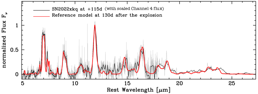
Figure 14: Comparison between the synthetic and observed MIR spectra of SN 2022xkq (black) where the flux in Channel 4 ($\lambda\geq 18$ $\mu$m) has been scaled to the model flux, with a wavelength-dependent scaling factor (see text).

5.2.1 Probing the Ionization and Abundance Structure

The comparison between the observed MIR spectrum, the spectrum of our reference model, and a low-density model is shown in Figure 15. Only the reference model matches the observations. As a reminder, the lines matching strong observed features are already discussed in § 3 and Table 3. The full list of significant optical and IR transitions in the models are given in s 6 and 7, and some are marked in Figure 16. We compare $F_{\nu}$ because the line features depend on the lifetimes thus, $F_{\nu}$ provides the proper scaling. The spectra are normalized to the [Co III]-dominated feature at $11.888$ $\mu$m. From the absolute flux in our models, the normalization factor required to match the [Co III]-dominated feature at $11.888$ $\mu$m corresponds to a distance modulus $\mu=32.51$ mag. This is remarkably similar to the distance modulus derived from SN independent methods, which find $\mu=32.46\pm 0.15$ mag (Pearson et al., 2023).

Table 6: Infrared Line Identifications at Day 130 in Reference Model

S	$\lambda$ [$\mu$m ]	Ion	S	$\lambda$ [$\mu$m ]	Ion	S	$\lambda$ [$\mu$m ]	Ion	S	$\lambda$ [$\mu$m ]	Ion	S	$\lambda$ [$\mu$m ]	Ion
$\ast\$	1.3209	[Fe II]		2.2187	[Fe III]	$\ast\$	5.6870†	[V I]	$\ast\ \ast\$	11.130	[Ni IV]	$\ast\$	21.829	[Ar III]
	1.3210	[Fe I]		2.2425	[Fe III]	$\ast\$	5.7044	[Co II]		11.167	[Co II]	$\ast\$	22.297	[Fe I]
$\ast\$	1.3281	[Fe II]		2.2443	[Fe II]		5.7391	[Fe II]	$\ast\$	11.238†	[Ti II]		22.80†	[Co IV]
	1.3422	[Fe I]		2.3086	[Ni II]		5.8933	[Ni I]		11.307	[Ni I]	$\ast\$	22.902	[Fe II]
	1.3556	[Fe I]		2.3486	[Fe III]		5.9395	[Co II]	$\ast\ \ast\ \ast\$	11.888	[Co III]	$\ast\ \ast\ \ast\$	22.925	[Fe III]
	1.3676	[Fe I]		2.3695	[Ni II]		5.9527	[Ni II]	$\ast\ \ast\$	12.001	[Ni I]		23.086	[Ni II]
$\ast\$	1.3722	[Fe II]		2.4139	[Co I]	$\ast\ \ast\$	6.2135	[Co II]	$\ast\$	12.1592†	[Ti II]	$\ast\$	23.196	[Co II]
	1.3733	[Fe I]	$\ast\$	2.5255	[Co I]		6.2730	[ Co I]	$\ast\ \ast\$	12.255	[Co I]		23.389	[Fe III]
	1.3762	[Fe I]		2.6521	[Co I]		6.2738	[Co II]	$\ast\$	12.2610	[Mn II]		24.04†	[Co IV]
	1.4055	[Co II]		2.7256	[Co I]		6.3683	[Ar III]	$\ast\ \ast\$	12.286†	[Fe II]	$\ast\ \ast\$	24.042	[Fe I]
$\ast\$	1.4434	[Fe I]	$\ast\$	2.8713	[Co I]		6.379	[Fe II]	$\ast\ \ast\$	12.642	[Fe II]	$\ast\ \ast\ \ast\$	24.070	[Co III]
$\ast\$	1.4972	[Co II]		2.8742	[Fe III]	$\ast\ \ast\ \ast\$	6.6360	[Ni II]	$\ast\$	12.681	[Co III]	$\ast\ \ast\ \ast\$	24.519	[Fe II]
$\ast\ \ast\$	1.5339	[Fe II]		2.9048	[Fe III]		6.7213	[Fe II]	$\ast\ \ast\$	12.729	[Ni II]		24.847	[Co I]
$\ast\ \ast\ \ast\$	1.5474	[Co II]	$\ast\ \ast\$	2.9114	[Ni II]	$\ast\ \ast\$	6.9196	[Ni II]	$\ast\ \ast\$	12.729	[Ni II]	$\ast\ \ast\ \ast\$	25.249	[S I]
	1.5488	[Co III]	$\ast\$	2.9542	[Co I]	$\ast\ \ast\ \ast\$	6.9853	[Ar II]	$\ast\$	12.811	[Ne II]	$\ast\ \ast\$	25.689	[Co II]
	1.5694	[Co II]		3.0060	[Co I]		7.0454	[Co I]		13.058	[Co I]	$\ast\ \ast\$	25.890	[O IV]
$\ast\ \ast\$	1.5999	[Fe II]		3.0305	[Co I]	$\ast\$	7.103	[Co III]		13.820	[Co III]		25.986	[Co II]
	1.6073	[Si I]		3.0439	[Fe III]	$\ast\$	7.1473	[Fe III]		13.924†	[Co IV]	$\ast\ \ast\ \ast\$	25.988	[Fe II]
$\ast\$	1.6267	[Co II]		3.0457	[Co I]		7.2019	[Co I]		14.006	[Co III]		26.100	[Co III]
$\ast\$	1.6347	[Co II]	$\ast\ \ast\ \ast\$	3.1200	[Ni I]	$\ast\$	7.3492	[Ni III]		14.356	[Co I]		26.130	[Fe III]
$\ast\ \ast\ \ast\$	1.6440	[Fe II]		3.2294	[Fe III]	$\ast\ \ast\$	7.5066	[Ni I]		14.391	[Co I]		26.601	[Fe II]
$\ast\$	1.6459	[Si I]		3.3942	[Ni III]	$\ast\$	7.7906	[Fe III]	$\ast\ \ast\$	14.739	[Co II]		27.530	[Co II]
$\ast\ \ast\$	1.6642	[Fe II]		3.4917	[Co III]	$\ast\$	8.044	[Co I]	$\ast\$	14.8140	[Ni I]		27.550	[Co I]
$\ast\$	1.6773	[Fe II]	$\ast\$	3.6334	[Co I]	$\ast\$	8.211	[Fe III]	$\ast\ \ast\$	14.977	[Co II]		28.466	[Fe I]
$\ast\$	1.7116	[Fe II]		3.7498	[Co I]		8.2825	[Co I]	$\ast\ \ast\ \ast\$	15.459	[Co II]		29.675	[Mn II]
$\ast\$	1.7289	[Co II]		3.8023	[Ni III]	$\ast\$	8.2993	[Fe II]		16.299	[Co II]	$\ast\ \ast\ \ast\$	33.038	[Fe III]
$\ast\$	1.7366	[Co II]	$\ast\ \ast\$	3.9524	[Ni I]	$\ast\ \ast\ \ast\$	8.405	[Ni IV]	$\ast\ \ast\ \ast\$	16.391	[Co III]		33.481	[S III]
	1.7413	[Co III]	$\ast\ \ast\ \ast\$	4.0763	[Fe II]	$\ast\$	8.6107	[Fe III]	$\ast\$	16.925	[Co I]		34.660	[Fe II]
$\ast\$	1.7454	[Fe II]		4.0820	[Fe II]	$\ast\$	8.6438	[Co II]	$\ast\ \ast\ \ast\$	17.936	[Fe II]	$\ast\$	34.713	[Fe I]
$\ast\$	1.7976	[Fe II]	$\ast\ \ast\$	4.1150	[Fe II]	$\ast\$	8.7325	[Fe II]	$\ast\$	18.2410	[Ni II]	$\ast\ \ast\ \ast\$	34.815	[Si II]
$\ast\$	1.8005	[Fe II]	$\ast\$	4.3071	[Co II]	$\ast\$	8.9147†	[Ti II]		18.265	[Co I]	$\ast\ \ast\ \ast\$	35.349	[Fe II]
$\ast\$	1.8099	[Fe II]		4.5196	[Ni I]	$\ast\ \ast\$	8.945	[Ni IV]	$\ast\$	18.390	[Co II]	$\ast\$	35.777	[Fe II]
	1.8119	[Fe II]	$\ast\ \ast\$	4.6077	[Fe II]	$\ast\ \ast\ \ast\$	8.9914	[Ar III]	$\ast\ \ast\ \ast\$	18.713	[S III]		38.801	[Fe I]
$\ast\$	1.9040	[Co II]	$\ast\ \ast\$	4.7881	[Ni I]	$\ast\$	9.1969†	[Ti II]	$\ast\ \ast\$	18.804	[Co II]		39.272	[Co II]
$\ast\ \ast\$	1.9393	[Ni II]		4.8603	[Fe III]		9.279†	[Co IV]		18.985	[Co II]	$\ast\ \ast\ \ast\$	51.301	[Fe II]
	1.9581	[Co III]	$\ast\ \ast\$	4.8891	[Fe II]	$\ast\$	9.618	[Ni II]	$\ast\$	19.0070	[Fe II]	$\ast\ \ast\ \ast\$	51.770	[Fe III]
	2.0028	[Co III]		5.0623	[Co I]		9.8195	[Co I]	$\ast\ \ast\$	19.056	[Fe II]		54.311	[Fe I]
	2.0073	[Fe II]		5.1635	[Co I]	$\ast\$	10.080	[Ni II]		19.138	[Ni II]	$\ast\$	56.311	[S I]
	2.0418	[Ti II]	$\ast\$	5.1796	[Co II]	$\ast\ \ast\$	10.1637†	[Ti II]		19.232	[Fe III]		60.128	[Fe II]
$\ast\$	2.0466	[Fe II]	$\ast\ \ast\$	5.1865	[Ni II]	$\ast\ \ast\$	10.1890	[Fe II]		20.167	[Fe III]
	2.0492	[Ni II]		5.2112	[Co I]		10.2030	[Fe III]		20.928†	[Fe II]
	2.0979	[Co III]		5.3402	[Fe II]	$\ast\$	10.5105	[Ti II]		21.17†	[Fe I]
	2.1334	[Fe II]		5.4394	[Co II]	$\ast\$	10.5105	[S IV]		21.986†	[Fe II]
	2.1457	[Fe III]		5.4652†	[V I]	$\ast\ \ast\ \ast\$	10.523	[Co II]		22.106†	[Ni I]
	2.1605	[Ti II]	$\ast\$	5.6739	[Fe II]	$\ast\ \ast\$	10.682	[Ni II]	$\ast\$	21.4810	[Fe II]

Note. — The relative strengths are indicated by the number of $*$. For transitions without known lifetimes (marked by ^†), $A_{i,j}$ are assumed from the equivalent iron levels. The transitions observed in SN 2022xkq above the threshold flux level are listed in Table 3.

Note, that the underlying continuum flux is dominated by a quasi-continuum (Karp et al., 1977; Hoeflich et al., 1993; Hillier & Dessart, 2012) produced by allowed line transitions, electron scattering and free-free radiation in a scattering-dominated MIR photosphere expanding with a velocity of about 1,500 to 2,000 km s^-1, and particle densities of $\approx 1-2\times 10^{7}$ cm^-3 which are close to the critical density for collisional de-excitation. Note that, based on non-LTE models, this effect was taken into account for the interpretation of many nebular spectra (e.g., Höflich et al., 2004; Telesco et al., 2015; Diamond et al., 2015, 2018; DerKacy et al., 2023). The high particle density and the presence of a photosphere leads to weaker features in ⁵⁸Ni than expected otherwise and potentially, blocks the emission of the most neutron-rich isotopes that form when $\rho_{c}$ is high. These isotopes have been observed in SN 2016hnk (Galbany et al., 2019), and may be observed in spectra of SN 2022xkq at later epochs. Moreover, the presence of a photosphere blocks part of the redshifted emission of forbidden lines formed in the outer optically thin layers. This leads both to a blue-shift vs. the rest-wavelengths of transitions formed close to the photosphere (compare Figure 16 and Table 6) for SN 2022xkq. Due to the photosphere receding with time and the decreasing blocking of the red-shifted emission components, the width of features by singly and doubly ionized transitions increases with time (Penney & Hoeflich, 2014) as been observed in many SNe, for example, [Fe II] 1.644 $\mu$m in SN 2014J and [Co III] 11.888 $\mu$m (Diamond et al., 2018; Telesco et al., 2015). This effect vanishes by day $\approx 200$. Note that, in general, the shift of both the blended and unblended features of SN 2022xkq and the models are consistent within the spectral resolution (Figure 15). Here, the blue-shifts in the almost unblended [Ni II] at 6.636 $\mu$m are $-460\pm 110$ km s^-1 in the observation (Figure 4) compared to $\sim-400$ km s^-1 in the model (Figure 16). Penney & Hoeflich (2014) found a shift of $\approx 2,000$ km s^-1 at day 100 for normal-luminosity models with a photosphere at $\approx 5,500$ km s^-1. The velocity shift is larger because the photosphere forms further out.

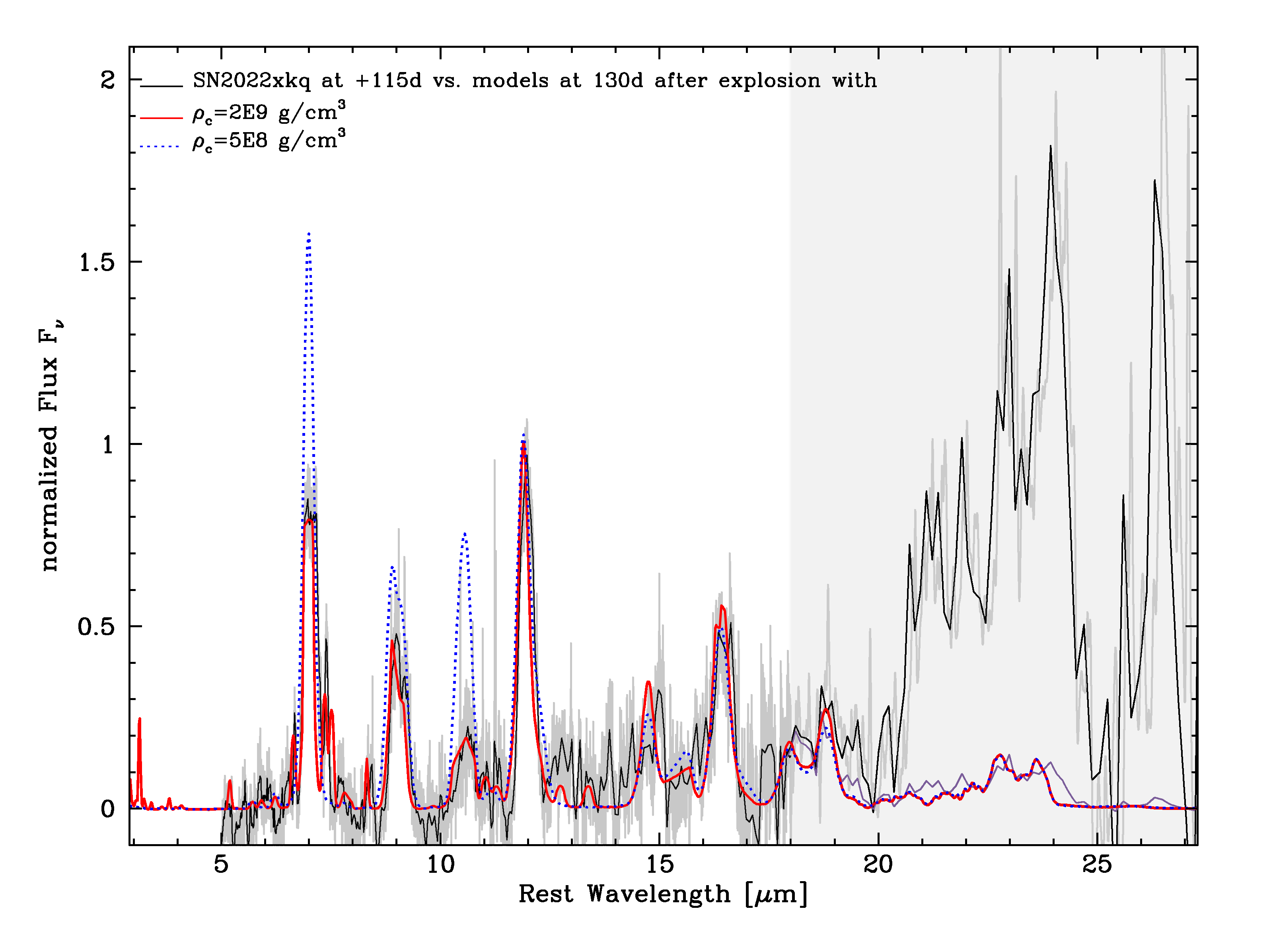
Figure 15: Comparison between the MIR spectra of SN 2022xkq in MIRI/MRS Channels 1–3 (solid black) and models with $\rho_{c}=~{}2\times 10^{9}$ g cm^-3 (solid red) and $5\times 10^{8}$ g cm^-3 (dotted blue) some 130 days after the explosion. The Channel 4 spectrum scaled to the flux level of the synthetic model spectrum using 3 $\mu$m-wide bins outside of the strong features is also shown (violet). The spectra in $F_{\nu}$ have been normalized to the peak of the [Co III] at 11.888 $\mu$m corresponding to a distance module of $32.52$ mag for our reference model. Note the strong [Ni I] feature at 3.12 $\mu$m in the models (see text). The low central density model strongly over-predicts the flux in the 7 and 9 $\mu$m [Ar] features as well as the 10.6 $\mu$m [Ni II]/[Co II] blend because the energy input is shifted to higher density material. Higher density models show smaller effects on the spectrum than low-density models (see text).

Another effect of the presence of the photosphere is a slight asymmetry in the line profile, not to be mistaken with overall asymmetries in the ejecta (Penney & Hoeflich, 2014). Overall, the synthetic and observed spectra agree well (Figure 16). Most features are blended with weak transitions (Table 6). The main features in the model are at 7 $\mu$m ([Ar II], [Ni i– iii]), 9 $\mu$m ([Ar III], [Ni IV]), a group at 10.6 $\mu$m ([S IV], [Co II], [Ni IV]), 11.8 $\mu$m ([Co III], with some [Co I] and [Fe II]), 14.8–16.0 $\mu$m ([Co II], [Co III]], [Fe II]), $16.3$ [Co III], [Fe II], and 17.5–19 $\mu$m ([Fe II], [S III]. Additionally, some weaker features of [Ti II] can be seen at 9.19 $\mu$m (Table 6), expected for lower luminosity SNe Ia, and placing SN 2022xkq at the lower end of transitional SNe Ia.

In Channel 4, the strong features only become apparent in the spectrum of SN 2022xkq after scaling the flux by the synthetic spectrum (Figure 17). The scaling factor is wavelength dependent and varies from a value of about 1 at 18 $\mu$m to about 50 at 26 $\mu$m. Overall, the spectra in Channel 4 are dominated by blends of singly and doubly ionized Fe and Co with peaks at $\sim$18, 23 and 24 $\mu$m. In our models, the [S III] at 18.713 $\mu$m dominates the feature at 19 $\mu$m. Mixing on scales of the positron mean free path, would further enhance this feature. The effect is similar to results on the photospheric S I at 1.0821 $\mu$m (Diamond et al., 2015). Even without mixing, the [S III] feature is an indication of a massive progenitor. M_Ch models produce a large amount of intermediate mass elements (IMEs) at the expense ejecta undergoing burning to NSE. In the models, we see a hint of the [S I] feature at 25 $\mu$m. It is not prominent because the direct and significant heating by $\gamma$-rays leads to mostly ionized S II (Figure 13). This feature is expected to grow with time as heating will transition from $\gamma$-rays to positrons by $\approx 200-300$ days. At wavelengths longwards of 18 $\mu$m, the appearance of [S III] is a direct consequence of the large amount of Si and S characteristic of M_Ch scenarios. Note the possible importance of high S/N observations in the MIRI/MRS Channel 4 to probe for $\rho_{c}$ larger than $4\times 10^{9}$ g cm^-3, because lines of [Cr V] and [Mn IV] would appear at 19.62 and 22.08 $\mu$m, respectively.

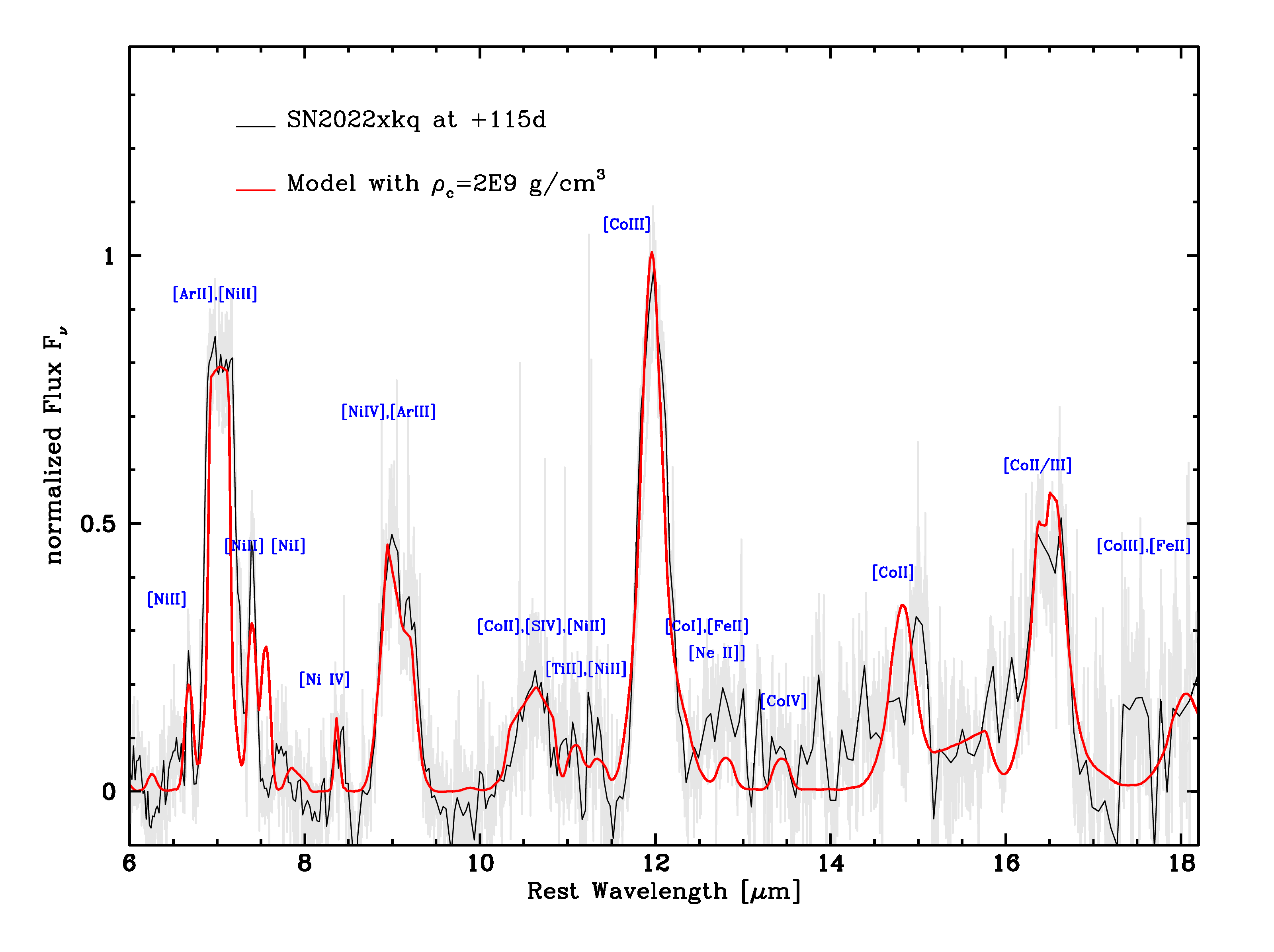
Figure 16: Same as Figure 15 with the observed spectrum for Channels 1-3 compared to the reference model, but with a tighter wavelength range. Strong features relevant for our interpretation are labeled. Note that many are blends (Table 6). Overall, the profiles of the synthetic and observed features are in good agreement. The peaks of many lines that form close to the photosphere are blue-shifted due to the blocking effect of the photosphere. However, the synthetic [Ni I] line at $\approx 7.5$ $\mu$m and [Ni II] at $\approx 7.4~{}$$\mu$m are too strong and slightly too weak, respectively compared to the observations, suggesting a slightly higher non-thermal excitation in the center of SN 2022xkq than predicted by the model, or inhomogeneous mixing.

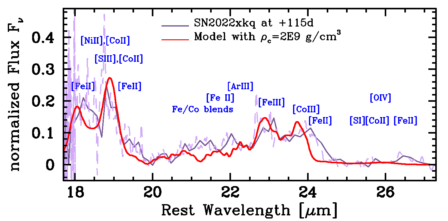
Figure 17: Same as Figure 15 with the observed, calibrated spectrum in Channel 4 with (violet) and without smoothing (light violet) compared to the reference model (red). Strong features relevant for our interpretation are labeled. Note that many are blends (Table 6). Overall, the synthetic and observed strong features are in reasonable agreement. Note the strong [S III] is indicative for a high mass WD (see text).

For many of the elements, multiple ionization stages are present, which lends support to the ionization structure discussed above. Within M_Ch scenarios, lower densities significantly degrade the fit by boosting the emission by features dominated by [Co II] at $10.6$ $\mu$m. In our models, lower $\rho_{c}$ results in more heating by ⁵⁶Co at lower velocity as the size of the electron capture region recedes. This shifts a significant amount of energy input into the high density region with the lower ionization stage dominating (Figure 13) shifting the [Co III]/[Co II] ratio. With the spectra normalized to [Co III] and little effect due to Ar, the corresponding features (e.g. 7, 9 $\mu$m) appear more prominent.

Our best fit model produces $\sim 6\times 10^{-2}$ M_⊙ of ⁵⁸Ni. About 50% of it is located within the photosphere. Mixing of the innermost regions may expose a larger fraction of the ⁵⁸Ni but, as discussed below, the narrow Ni lines put strong limits on extended mixing. Note that we cannot exclude higher central density models as used in Galbany et al. (2019) because the highest-density burning layers, with the lowest electron/neutron ratio, $Y_{e}$ would be hidden below the photosphere (see Figs. 25-26 in Galbany et al., 2019). The [Ni I] line at about 7.5 $\mu$m is predicted by the model, but is clearly absent in the observation. To reproduce the model prediction of [Ni I] it would have to be blue-shifted by $\approx 2,500$ km s^-1 and blended (Figure 16). The shift of [Ni I] in the inner, high-density layers is due to recombination rates that depend on $\rho^{2}$. Higher $\rho_{c}$ does not necessarily produce significantly more ⁵⁸Ni because the nuclear statistical equilibrium shifts to more neutron-rich isotopes (see Fig. 25 in Galbany et al., 2019). If the ⁵⁸Ni forms a shell it would be unstable to Rayleigh-Taylor (RT) mixing. Without detailed simulations, the impact on the line profile is hard to predict. The difference between the models and data, can be due to several effects: (1) a higher $\rho_{c}$ and a corresponding shift towards more neutron-rich isotopes reducing $Y_{e}$, (Brachwitz et al., 2000; Höflich et al., 1998; Hristov et al., 2021); (2) some moderate, inhomogeneous mixing (Fesen et al., 2015); and (3) some passive drag by a turbulent field produced during the smoldering phase when the flame speed is low (close to the laminar speed) for $\approx 1-2$ s prior to central ignition (Khokhlov, 1995; Khokhlov et al., 1997b; Domínguez & Höflich, 2000). See the velocity field shown in Fig. 9 of Höflich & Stein (2002). These effects may be reproduced in a finely tuned model, which is beyond the scope of this work. We abstain from further tuning $\rho_{c}$ due to the lack of high S/N spectra beyond 18 $\mu$m needed to verify the presence of neutron rich isotopes (see C. Ashall et al. 2023, in prep.).

5.2.2 Line Profiles

Figure 16 shows the model and observed spectra, with some of the stronger features identified. Ni lines appear from neutral through triply ionized ions. Peaked profiles for iron-group elements are the direct result of the energy input being dominated by $\gamma$-rays (Figure 16). The model predicts the correct line widths of [Co II] and [Co III].

The 7 and 9 $\mu$m features are both dominated by Ar and blended by [Ni II], but the 9 $\mu$m feature is heavily blended with [Ni IV]. Compared to normal-luminosity SNe Ia, the Ar layers are expanding at lower velocities. Within M_Ch explosions, this can be understood as a consequence of the dominant production of quasi statistical equilibrium in low luminosity supernovae. As a consequence, in sub-luminous SNe, Ar (and Ca) are elements formed during the breakout to NSE and appear at lower velocities, resulting in narrower profiles. The profile is mostly flat, but narrower compared to previously observed normal-luminosity SN Ia (Figure 7). As a result, the Ni features in the blue end of the 7 $\mu$m profile are well separated from the strongest [Ni II] line at 6.636 $\mu$m though somewhat contaminated by the weak Ni II at 6.920 $\mu$m. Note that the [Ar II]-dominated 7 $\mu$m feature has a ‘dome-shaped’ rounded top produced by a narrow line blending rather than asymmetry, with a velocity corresponding to $\approx 3,800$ km s^-1, consistent with the central hole in the argon distribution (Figure 12). The 7 $\mu$m feature is slightly too narrow compared to the observation, which may indicate some RT driven mixing. In the model, the dome shape is produced by [Ni II]. While our models cannot explicitly discriminate between whether the dome shape is due to the [Ni II] blend or if the model is slightly too dim, the presence of the small [Ni I] feature suggests that it is slightly too dim.

In contrast, the 9 $\mu$m [Ar II] profile is heavily distorted/tilted by ‘low velocity’ [Ni IV] (and some [Ti II]). The synthetic and the observed profiles are due to blending. The result is an asymmetric, peaked profile, making it unusable as an indicator for chemical asymmetry in the explosion.

The narrower [Co III] at 11.888 $\mu$m found in SN 2022xkq as compared to normal-luminosity SNe Ia is consistent with the fact that the NSE region becomes more concentrated towards the inner region in under-luminous SNe Ia; or more precisely, the QSE region grows at the expense of NSE elements (Hoeflich & Khokhlov, 1996; Mazzali et al., 2020; Höflich et al., 2002a; Ashall et al., 2018) (see also § 4.2.3). It is amplified by the blocking due to the photosphere that cuts off parts of the red-shifted contribution to the line emission (see § 5.2.1).

The model successfully reproduces the narrow [Ni II] and [Ni IV] lines observed providing a possible path to probing the physics of the thermonuclear runaway. Within the framework of M_Ch explosions, the ignition process and its location is highly debated, ranging from central ignition (Khokhlov et al., 1993; Gamezo et al., 2003) to multi-spot ignition in $\approx 100$ spots distributed over more than a hundred km (Seitenzahl et al., 2013). Detailed simulations of the simmering phase suggest a single-spot ignition close to the center at $\approx 35-50$ km s^-1 (Höflich et al., 2002a; Zingale et al., 2011), but possibly out to 100 km s^-1 (Zingale et al., 2011). For the normal bright SN 2021aefx, Blondin et al. (2023) found that the delayed detonation model based on a strong off-center multi-spot ignition (Seitenzahl et al., 2013) fails to reproduce the strength of Ni lines by factors of 2 to 3, whereas delayed-detonation models starting from a single-spot ignition can reproduce the Ni lines within the model uncertainties (DerKacy et al., 2023). For SN 2022xkq, we find good agreement in the Ni lines with single spot ignition. Because the early deflagration phase may be similar, this may indicate that single-spot ignition is common.

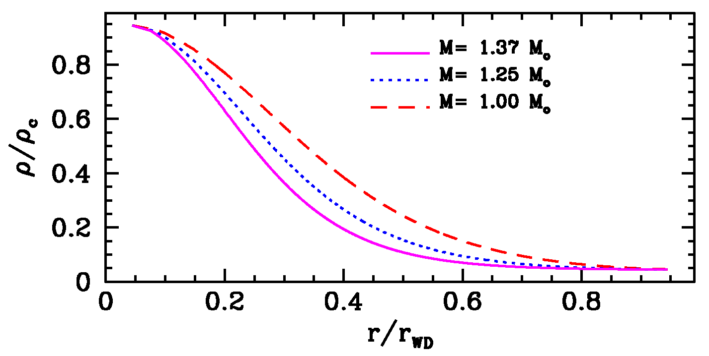
Figure 18: Normalized density as a function of radius. With increasing mass, they become more centrally concentrated (from Hoeflich, 2017). Note that M(WD) $\approx 1.25$ M_⊙ is the dividing line between M_Ch and sub-M_Ch explosions.

5.2.3 Alternative Scenarios

Detailed spectral fits of a wide variety of scenarios is beyond the scope of this paper, but constraints can be found by combining spectral indicators.

The observed [Co II]/[Co III] ratio requires high $\rho_{c}$, compared to normal-luminosity SNe Ia (Diamond et al., 2015; Telesco et al., 2015; Diamond et al., 2018) in M_Ch explosions because, more electron capture shifts the emission powered by radioactive decays towards lower densities. In contrast, for sub-M_Ch mass explosions such as helium-triggered detonations (Shen et al., 2018; Polin et al., 2019; Boos et al., 2021) or low density mergers (García-Berro et al., 2017), lowering M_WD and $\rho_{c}$ will decrease the average density of spectral formation, reducing the average [Co II]/[Co III] ratio. One of the effects that changes the ionization balance is the overall flatter density distribution in the initial sub-M_Ch WD (see Figure 18), the other is the lowering of binding energy with decreasing M_WD, which changes the velocity distribution of the ejecta. Sub-M_Ch explosions can produce an under-luminous SNe Ia like SN 2022xkq for progenitors with $0.9\leq M_{WD}\leq 1.0$ M_⊙, but the central densities are too low for the production of electron capture elements. However, stable Ni is seen in SN 2022xkq.

In the case of a sub-M_Ch WD, a low $Y_{e}$ may be inherited from the progenitor, due to an overabundance of ²²Ne produced during the stellar burning in massive stars. As suggested by Blondin et al. (2022), super-solar metallicity will shift $Y_{e}$ resulting in the production of ⁵⁸Ni in ⁵⁶Ni in the QSE regions resulting in ⁵⁸Ni features as broad as the nebular ⁵⁶Co line. However, the Ni lines in SN 2022xkq are narrow (FWHM $\approx 2,500$ km s^-1, s 4 and 16) rather having a FWHM of $\approx 10,000$ km s^-1 (see e.g. Shen et al., 2018), excluding this path.

Alternatively, a low $Y_{e}$ and thus, some central Ni may be produced in sub-M_Ch progenitor systems that contain very old WDs. Over time scales of $\sim 5$ billion years, gravitationally driven diffusion may allow ²²Ne settling in the core of a crystallized WD (Deloye & Bildsten, 2002). For an initial composition of solar metallicity, the amount may or may not be sufficient to account for some [Ni II] emission observed at about 1.9 $\mu$m in some other SNe Ia (e.g., Friesen et al., 2014; Diamond et al., 2015; Hoeflich et al., 2021; Blondin et al., 2023). However, in SN 2022xkq, we see Ni in all ionization stages. The amount of stable Ni produced in old, low mass WDs is too small by a factor of 3–4 to account for the observed line strengths. The factor needs to be even larger because old stars in spiral galaxies have sub-solar metallicities. Moreover, the ⁵⁸Ni would settle at velocities below the photosphere at 130 days after the explosion, requiring mixing.

Other alternative scenarios are dynamical mergers of two WDs where the C/O is ignited on dynamical time-scales by interaction: a) starting with grazing incidence (classical mergers), b) violent mergers, or c) direct collisions (Benz et al., 1990; Rosswog et al., 2009; Kushnir et al., 2013; Pakmor et al., 2013; García-Berro et al., 2017). All three would lead to asymmetric envelopes in density or abundance structures.

Unlike the 35 normal-bright SNe Ia (Cikota et al., 2019) for which polarization has been observed, the under-luminous SN 1999by and SN 2005ke show a qualitatively different polarization spectrum around peak brightness, indicating an overall rotationally symmetric photosphere with an axis ratio of $\approx 0.9$ based on detailed non-LTE models (Howell, 2001; Patat et al., 2012). Dynamical mergers have been suggested and discussed as possible alternatives to M_Ch explosions of rapidly rotating WDs opening up the possibility that under-luminous SNe Ia are a population distinct from normal-bright SNe Ia (Patat et al., 2012; Hoeflich et al., 2023). So far, no late-time spectropolarimetry has been obtained for under-luminous SNe Ia that would produce the flip in the polarization angle in configurations found in head-on collisions of two WDs (Höflich, 1995; Bulla et al., 2016).

The intermediate state in classical mergers (for almost all mass ratios between the WDs) produces a puffed up, low density quasi-hydrostatic phase without the production of a significant amount of stable Ni (for a review, see García-Berro et al., 2017). However, violent mergers can produce a lot of ⁵⁸Ni and show strong MIR Ni features. In fact, the strength of the Ni features far exceed the observations of the over-luminous SN 2023pul (Kwok et al., 2023b) and the under-luminous SN 2022xkq. For both SNe Ia in the MIR, the observed MIR [Ar II] lines are too strong and the MIR Ni features are too weak compared to the model by an order of magnitude. However, it is unclear whether this is a generic property of this class of explosions.

A direct collision with parameters closer to those suggested for the under-luminous SN 2007on may be more likely (Mazzali et al., 2018). This scenario, however, resulted in the ignition of both WDs, a ‘double line’ pattern in all elements and a significant shift in Ni ($\approx 1,500-3,000$ km s^-1, Dong et al., 2015; Mazzali et al., 2018; Vallely et al., 2020). Neither of these effects are compatible with SN 2022xkq unless seen ‘equator on’. In addition, we see only one component in the narrow Ni line severely limiting even small deviations from the equatorial viewing direction, unless only one of the WDs is close to M_Ch. We note that polarization spectra and their evolution would be very unlike the two under-luminous SNe Ia mentioned above. We consider WD collisions as the explosion mechanism for SN 2022xkq to be unlikely, but without detailed modeling (beyond the scope of this work) cannot definitely rule them out.

6 Results

The main findings of our analysis are as follows:

• The spectrum of the under-luminous SN 2022xkq is distinct compared to spectra of normal-luminosity SNe Ia. The MRS/MIRI spectrum permits many detailed inferences including the first lines identified beyond 14 $\mu$m in SN Ia observations. These newly identified lines include [Co II]-dominated blends between 14–17 $\mu$m, and complex blends of several iron-group elements with contributions from [S III], [Ar II], [S I], and [O IV] at $\lambda>18$ $\mu$m.

• The identification of [Ti II] lines in the blended MIR features are consistent with SN 2022xkq being an under-luminous SN Ia.

• The stronger ratio of [Ar II]/[Ar III] in SN 2022xkq relative to the normal-luminosity spectra at similar epochs suggests a shift in the ionization balance toward singly ionized species over doubly ionized ones.

• In observations at these phases, line formation is a complex mixture of allowed lines, forbidden transitions, a pseudo-continuum, and other radiative transfer effects. The combination of fits and data driven measurements to the [Ni II] 6.636 $\mu$m, [Ni III] 7.349 $\mu$m, and [Co III] 11.888 $\mu$m lines reveal: a) that the peaks of the IGEs are blue-shifted by $\sim 200-400$ km s^-1 relative to the rest wavelength of the dominant line; and b) that these features are narrow in width when compared to the same lines in normal-luminosity SNe Ia. Fitting of the line profiles with simple analytic functions (e.g. Gaussians) must be approached with caution as they do not capture the complex line formation physics, even in some isolated lines with little blending.

• A tentative correlation is seen between the FWHM of the [Co III] 11.888 $\mu$m resonance line and the light curve shape parameter $\Delta{\rm m_{15}(B)}$. This relationship is consistent with the ⁵⁶Ni being produced in NSE burning occurring closer to the center in under-luminous objects. Future MIR observations should continue to add to this plot to see if it follows the luminosity-width relation observed in the optical.

• The light curve properties (Table 5) of the model are consistent with the early-time data of SN 2022xkq (Pearson et al., 2023), as well as other under-luminous SNe Ia such as SN 2007on and SN 2011iv (Gall et al., 2018). While SN 2022xkq is at the lower luminosity end of the transitional SNe Ia distribution, it is significantly (1.5 mag), brighter, than SN 1991bg-like objects (§ 5).

• The spectral characteristics can be understood within the framework of high-density burning in a delayed-detonation model in which somewhat more mass is consumed in the deflagration prior to the onset of the DDT, seen equator on (Figure 15). In particular, the shift from a predominately doubly ionized spectrum to a mix of ionization I-III is consistent with the low luminosity. The shift in the ionization balance towards lower stages is obvious (Figure 13 and § 5.2.1). Moreover, the strongest features in the models are also the strongest features observed, and all weak features in the observations have their equivalent in the model (compare Table 3 with Table 6).

• Electron capture in the central region has a significant impact on the spectra: With increasing $\rho_{c}$, the higher average density shifts the ionization balance from [Co III] to [Co II]. As a result, the [Co II] lines are stronger (Figure 15). Furthermore, the large number of Ni features indicates electron capture (Table 6).

• The sensitivity of intermediate mass vs. iron-group elements and the important role of high resolution in the MIR accessible with JWST has been demonstrated as a key to constrain the underlying physics and to test models (Figure 15).

• At $\sim$130 days after explosion, the spectra form during the onset of the nebular phase. In our models, the optical to MIR photosphere is formed by a quasi-continuum at $\approx 2,000~{}$km s^-1 hiding the innermost layers. This photospheric blocking is consistent with the shift of the peak of the emission features relative to the rest wavelength by a few hundred km s^-1 (s 7 and 16). As discussed in § 5.1, only some of the electron capture elements in the models are above the photosphere and potentially, electron capture elements such as Cr, and Mn are hidden. Within the framework of M_Ch mass explosions, the central density of the WD $\rho_{c}=2\times 10^{9}$ g cm^-3 and the ⁵⁸Ni mass may be regarded as a lower limit.

• SN 2022xkq is likely to have been observed close to ‘equator-on’ and/or the point of the DDT is within the low-velocity distribution of ⁵⁶Ni (s 5.2.1 and 5.2.2). Line polarization should be largest when seen from near to the equator, but vanishes when seen from other inclinations showing the importance of spectropolarimetry during the photospheric phase.

• The line profiles of [Ar II] and [Co III] show a narrow flat top and are rounded, respectively. This is expected from under-luminous models for the explosion of a massive WD with large pre-expansion during the deflagration phase prior to the DDT, resulting in overall an increased production of IMEs (Si/S/Ca/Ar) compared to that produced in normal-luminosity SNe Ia (Figure 7).

• The [Ar III] profile at 9 $\mu$m is strongly tilted because it is contaminated by Ti and Ni blends. In under-luminous SNe Ia, it cannot be used to infer asymmetry in the density distribution (§ 5.2.2).

• The line profile of [Ar II] at 7 $\mu$m is better suited to deciphering the location of the DDT and the viewing angle of under-luminous SN Ia. This is because line-blending is reduced due to the lower overall velocities. The size of the ‘Ar hole’ is slightly smaller in our models than inferred from the observations, but suggests that SN 2022xkq is seen from the equator. The domed-shaped profile is a result of line-blending and not asymmetry (§ 5.2.2).

• The [Co III] feature at 11.888 $\mu$m shows a rounded, broad profile characteristic for a central ⁵⁶Ni-free region. This is also supported by and consistent with the numerous narrow ⁵⁸Ni lines (§ 5.2.1).

• The strong [S III] at $\approx 19$ $\mu$m is indicative of a massive WD, as in under-luminous SNe Ia the IME production is increased compared to normal-luminosity SNe Ia (see s 14 and 17).

• In under-luminous SNe Ia, the ionization balance is shifted towards lower states (Figure 13) and in the central region, neutral IGEs become significant. This is also seen as a the lower half width of both electron capture lines and lines from neutral Fe, Co, Ni when compared to normal-luminosity SNe Ia.

• The lines of stable ⁵⁸Ni are clearly identified and are consistent between models and observations. At $\sim 130$ d past the explosion, the densities of the central region remained high, $>10^{7}$ g cm^-3 up to $\approx 2,000$ km s^-1 resulting in Ni emission less pronounced than expected in the nebular phase (§ 5). The narrow ⁵⁸Ni lines suggest a central ignition mixing of electron capture elements produced by pre-existing turbulent fields rather than by RT-instabilities as would be expected from multi-spot, off-center ignition (§ 5.2.2).

• A central DDT white C/O-rich material mixed-down can all but be excluded because the ⁵⁸Ni lines are narrow. For the first time, this may constrain the mechanisms possible for the DDT (s 5 and 5.2.2).

• The synthetic fluxes in MIR spectra (§ 5.2) are consistent with the observations of SN 2022xkq. The MIR has the advantage of insensitivity to reddening.

7 Discussion

Compared to previous low-resolution observations, the additional insight afforded by MIRI/MRS is readily apparent, especially as it relates to the increased wavelength coverage of MRS relative to LRS and the higher resolution. In SN 2022xkq, the additional wavelength coverage reveals multiple [Co]-dominated features in the 14–17 $\mu$m range, as well as complex blends of select transitions from [O], [S] and [Ar] along with many blended features comprised of [Fe], [Ni], and [Co] lines beyond $\sim 20$ $\mu$m.

The decrease in velocity errors from $\gtrsim 2,000$ km s^-1 to $\sim 100$ km s^-1 allows us to accurately measure small-scale velocity line shifts (see s 4, 5 and 6), to assess whether they originate from asymmetries (such as those originating from off-center DDTs), line formation effects, or temporal evolution from sources such as positron transport (at later epochs). This increased resolution also affords us the ability to better determine the shape of line profiles throughout the spectrum. In particular, the width and shape of the [Ar II] and [Ar III] lines from weak blends permits the estimation of the viewing angle of the supernova if observed at the appropriate epochs. Furthermore, these Ar lines probe the transition between the NSE and QSE regions during burning and provide clear discriminators between different explosion models. Finally, the increase in resolution compared to LRS data allows for previously blended lines to be resolved, such as the [Ni II] 6.636 $\mu$m and [Ni III] 7.349 $\mu$m lines. This provides tighter constraints on the physical conditions present in the ejecta.

The apparent correlation between the FWHM of the [Co III] 11.888 $\mu$m line and the light curve shape parameter offer tantalizing hope for the existence of a MIR spectroscopic luminosity-width relation that may be similar to the luminosity-width relation (Phillips, 1993). As more data are added to this plot, the relationship may provide an independent method to calculate the luminosity of a SN Ia with a single nebular phase spectrum. Over the coming years, as the sample of MIR spectra from JWST grows this relationship can be tested.

Unlike the traditional luminosity-width relation, determining whether a SN Ia meets the criteria for inclusion on the MIR luminosity-width plot (Figure 11) is less straightforward. In order for such a measurement to accurately probe this relation, the SN must be in the nebular phase with little to no contamination from an underlying photosphere, ⁵⁶Co decay must be the dominant source of energy deposition in the ejecta, and the strength of the weak blends of [Fe III] and [Ni I] should be low. In the context of M_Ch explosions, this phase will occur earlier in less luminous objects and later in more luminous ones. The specific timing of this window will vary from object to object due to differences in the physical conditions of the ejecta, but spectroscopic observations targeting the $\sim$100–300 day window should meet these conditions in most SNe Ia.

SN 2022xkq is one of the most extensively observed under-luminous SN Ia ever, with an early time data set starting hours after explosion and spanning from the ultraviolet to the near-infrared (Pearson et al., 2023). Yet, this extensive data set does not conclusively point towards a specific origin for SN 2022xkq. With the addition of the MIR observations presented here, a clearer picture emerges. The early time presence of carbon points towards unburnt material in the outer layers, which naturally arise in the M_Ch model presented here. The lack of bi-modality in the [Co III] 11.888 $\mu$m line and the MIR electron capture lines (e.g. ⁵⁸Ni) located interior to the ⁵⁶Ni region disfavor a collision; The lack of late-time O lines seen in the MIR, disfavors a merger; and the presence of strong electron capture lines favors high-density burning in the ejecta. This highlights the importance of multi-epoch, multi-wavelength observations of SNe Ia to determine the specific origins of individual objects.

Finally, we mention some limitations that will be overcome in the future. JWST is still in the early stages of operation. The data reduction and calibration will improve, in particular at longer wavelengths. Moreover, additional later-time spectra will be needed to see the innermost region. Due to both these effects, we could only obtain a lower limit upon electron capture elements such as Cr, Mn that have strong transitions beyond 18 $\mu$m. Detecting these lines would further refine the central density and the degree of mixing as these lines will only be present in models with $\rho_{c}\gtrsim 4\times 10^{9}$ g cm^-3. Estimates of the cross-sections for many transitions of iron group elements will be obtained by calibration of bright SNe Ia, as the cross-sections are not available for many transitions, for example those of [Ti II].

8 Conclusion

We present a MIRI MIR spectrum of the under-luminous SN Ia, SN 2022xkq, obtained at $+114.2$ d past maximum light. These are the first JWST observations of an under-luminous SN Ia and the first lines identified beyond 14 $\mu$m in SNe Ia observations. The data show evidence of isolated narrow lines of stable Ni emission, and strong emission from Ar and Co. In contrast to normal-luminosity SNe Ia, SN 2022xkq shows lower ionization states; in particular, it contains more [Ar II] relative to [Ar III]. Furthermore, the velocity extent of the resonance [Co III] feature is narrower compared to more luminous SNe Ia observed at roughly the same phase. This indicates the ⁵⁶Ni is closer to the core of the explosion. We also find a potential correlation between the FWHM of the [Co III] resonance feature and the light curve shape parameter $\Delta{\rm m_{15}(B)}$. Observing more SNe Ia at this phase will allow us to understand if this follows the luminosity-width relation for SNe Ia.

By comparing the data to newly synthesized non-LTE models we determine that the presence of narrow forbidden Ni lines is strong evidence for the explosion of a massive WD. The presence of multiple [Ti II] lines is consistent with SN 2022xkq’s location at the low luminosity end of this class. We show that the MIR spectra and the absolute flux can be well understood within an off-center delayed-detonation scenario seen equator on with a peak luminosity $\sim 1.2$ mag below normal SNe Ia. The spectra also hint that the SN had a central thermodynamic runaway and only a moderate off-set of the DDT. The strong IME elements and low luminosity suggest, at least in some SNe Ia, the lower luminosity is not correlated with a lower total WD mass.

This work demonstrates the power of using JWST data in combination with detailed simulations; especially, the wavelength coverage beyond 14 $\mu$m provided by MIRI/MRS. Looking ahead, harnessing this capability through forthcoming observations promises to usher us into a new era of SNe Ia physics.

Appendix A Optical lines at day 130 after the explosion

Table 7: Optical Line Identifications at Day 130 in Reference Model

S	$\lambda$ [$\mu$m ]	Ion	S	$\lambda$ [$\mu$m ]	Ion	S	$\lambda$ [$\mu$m ]	Ion	S	$\lambda$ [$\mu$m ]	Ion	S	$\lambda$ [$\mu$m ]	Ion
	0.3689	[Co II]		0.4641	[Fe II]		0.5562	[Co II]		0.8030	[Co II]		0.9697	[Co I]
	0.4104	[Co II]	$\ \ \ast\$	0.4659	[Fe III]	$\ \ \ast\$	0.5890	[Co III]	$\ \ast\ \ast\$	0.8123	[Co II]		0.9705	[Fe III]
	0.4154	[Co II]		0.4703	[Fe III]		0.5908	[Co III]		0.8123	[Co II]		0.9946	[Co II]
	0.4178	[Fe II]		0.4729	[Fe II]		0.6072	[Co I]		0.8303	[Ni II]	$\ast\ \ast\ \ast\$	0.9946	[Co II]
$\ \ \ast\$	0.4245	[Fe II]		0.4735	[Fe III]		0.6129	[Co III]		0.8336	[Co II]	$\ast\ \ast\ \ast\$	1.0191	[Co II]
	0.4246	[Fe II]		0.4749	[Co II]		0.6197	[Co III]		0.8466	[Co II]	$\ \ast\ \ast\$	1.0248	[Co II]
	0.4278	[Fe II]		0.4756	[Fe III]		0.6578	[Co III]		0.8469	[Co II]		1.0283	[Co II]
$\ \ \ast\$	0.4289	[Fe II]		0.4771	[Fe III]		0.6586	[Co I]		0.8502	[Ni III]	$\ \ \ast\$	1.0283	[Co II]
	0.4307	[Fe II]		0.4804	[Co II]		0.6669	[Ni II]		0.8546	[Co I]		1.0611	[Fe III]
	0.4321	[Fe II]		0.4882	[Fe III]		0.6855	[Co III]	$\ \ \ast\$	0.8574	[Co II]		1.0718	[Ni II]
	0.4327	[Ni II]		0.4891	[Fe II]		0.6934	[Co II]		0.8583	[Co II]		1.0718	[Ni II]
	0.4348	[Fe II]		0.4932	[Fe III]		0.7138	[Ar III]		0.8597	[Co I]	$\ \ast\ \ast\$	1.0824	[S I]
	0.4354	[Fe II]	$\ \ \ast\$	0.5013	[Fe III]		0.7155	[Co III]	$\ \ast\ \ast\$	0.8619	[Fe II]		1.0885	[Fe III]
	0.4360	[Fe II]		0.5086	[Fe III]	$\ \ast\ \ast\$	0.7157	[Fe II]	$\ \ \ast\$	0.8894	[Fe II]	$\ \ \ast\$	1.0976	[Co II]
	0.4361	[Fe II]		0.5113	[Fe II]	$\ \ \ast\$	0.7174	[Fe II]		0.9036	[Fe II]		1.0994	[Si I]
	0.4374	[Fe II]	$\ \ \ast\$	0.5160	[Fe II]		0.7249	[Co I]		0.9054	[Fe II]	$\ \ \ast\$	1.1283	[Co II]
	0.4415	[Fe II]		0.5222	[Fe II]	$\ \ast\ \ast\$	0.7293	[Ca II]		0.9071	[S III]	$\ \ \ast\$	1.1309	[S I]
	0.4418	[Fe II]	$\ \ \ast\$	0.5263	[Fe II]	$\ \ast\ \ast\$	0.7326	[Ca II]		0.9229	[Fe II]		1.1616	[Ni II]
	0.4453	[Fe II]		0.5270	[Co II]	$\ \ast\ \ast\$	0.7380	[Ni II]		0.9270	[Fe II]		1.2489	[Fe II]
	0.4459	[Fe II]	$\ \ \ast\$	0.5272	[Fe III]		0.7390	[Fe II]	$\ \ast\ \ast\$	0.9339	[Co II]		1.2525	[Fe II]
	0.4476	[Fe II]		0.5298	[Fe II]	$\ \ \ast\$	0.7414	[Ni II]	$\ast\ \ast\ \ast\$	0.9345	[Co II]	$\ast\ \ast\ \ast\$	1.2570	[Fe II]
	0.4490	[Fe II]		0.5335	[Fe II]	$\ \ \ast\$	0.7455	[Fe II]		0.9447	[Fe III]	$\ \ \ast\$	1.2707	[Fe II]
	0.4494	[Fe II]		0.5378	[Fe II]		0.7541	[Co II]		0.9474	[Fe II]	$\ \ \ast\$	1.2791	[Fe II]
	0.4501	[Co III]		0.5414	[Fe III]		0.7640	[Fe II]		0.9533	[S III]	$\ \ \ast\$	1.2946	[Fe II]
	0.4608	[Fe III]		0.5472	[Co II]		0.7689	[Fe II]		0.9642	[Co II]		1.2981	[Fe II]
	0.4624	[Co II]		0.5548	[Co II]		0.7892	[Ni III]	$\ \ \ast\$	0.9642	[Co II]

References

- Argyriou et al. (2023) Argyriou, I., Glasse, A., Law, D. R., et al. 2023, A&A, 675, A111, doi: 10.1051/0004-6361/202346489
- Arnett (1982) Arnett, W. D. 1982, ApJ, 253, 785, doi: 10.1086/159681
- Arnett et al. (1985) Arnett, W. D., Branch, D., & Wheeler, J. C. 1985, Nature, 314, 337, doi: 10.1038/314337a0
- Ashall et al. (2016a) Ashall, C., Mazzali, P., Sasdelli, M., & Prentice, S. J. 2016a, MNRAS, 460, 3529, doi: 10.1093/mnras/stw1214
- Ashall et al. (2016b) Ashall, C., Mazzali, P. A., Pian, E., & James, P. A. 2016b, MNRAS, 463, 1891, doi: 10.1093/mnras/stw2114
- Ashall et al. (2018) Ashall, C., Mazzali, P. A., Stritzinger, M. D., et al. 2018, MNRAS, 477, 153, doi: 10.1093/mnras/sty632
- Ashall et al. (2021) Ashall, C., Lu, J., Hsiao, E. Y., et al. 2021, ApJ, 922, 205, doi: 10.3847/1538-4357/ac19ac
- Astropy Collaboration et al. (2013) Astropy Collaboration, Robitaille, T. P., Tollerud, E. J., et al. 2013, A&A, 558, A33, doi: 10.1051/0004-6361/201322068
- Astropy Collaboration et al. (2018) Astropy Collaboration, Price-Whelan, A. M., Sipőcz, B. M., et al. 2018, AJ, 156, 123, doi: 10.3847/1538-3881/aabc4f
- Astropy Collaboration et al. (2022) Astropy Collaboration, Price-Whelan, A. M., Lim, P. L., et al. 2022, apj, 935, 167, doi: 10.3847/1538-4357/ac7c74
- Bell et al. (2004) Bell, J. B., Day, M. S., Rendleman, C. A., Woosley, S. E., & Zingale, M. 2004, ApJ, 606, 1029, doi: 10.1086/383023
- Benetti et al. (2005) Benetti, S., Cappellaro, E., Mazzali, P. A., et al. 2005, ApJ, 623, 1011, doi: 10.1086/428608
- Benz et al. (1990) Benz, W., Bowers, R. L., Cameron, A. G. W., & Press, W. H. . 1990, ApJ, 348, 647, doi: 10.1086/168273
- Blondin et al. (2022) Blondin, S., Bravo, E., Timmes, F. X., Dessart, L., & Hillier, D. J. 2022, A&A, 660, A96, doi: 10.1051/0004-6361/202142323
- Blondin et al. (2023) Blondin, S., Dessart, L., Hillier, D. J., Ramsbottom, C. A., & Storey, P. J. 2023, A&A, 678, A170, doi: 10.1051/0004-6361/202347147
- Bloom et al. (2012) Bloom, J. S., Kasen, D., Shen, K. J., et al. 2012, ApJ, 744, L17, doi: 10.1088/2041-8205/744/2/L17
- Boos et al. (2021) Boos, S. J., Townsley, D. M., Shen, K. J., Caldwell, S., & Miles, B. J. 2021, ApJ, 919, 126, doi: 10.3847/1538-4357/ac07a2
- Brachwitz et al. (2000) Brachwitz, F., Dean, D. J., Hix, W. R., et al. 2000, ApJ, 536, 934, doi: 10.1086/308968
- Branch et al. (1996) Branch, D., Romanishin, W., & Baron, E. 1996, ApJ, 465, 73, doi: 10.1086/177402
- Branch et al. (2006) Branch, D., Dang, L. C., Hall, N., et al. 2006, PASP, 118, 560, doi: 10.1086/502778
- Bravo et al. (2009) Bravo, E., García-Senz, D., Cabezón, R. M., & Domínguez, I. 2009, ApJ, 695, 1257, doi: 10.1088/0004-637X/695/2/1257
- Brooker et al. (2021) Brooker, E., Plewa, T., & Fenn, D. 2021, MNRAS, 501, L23, doi: 10.1093/mnrasl/slaa141
- Bulla et al. (2016) Bulla, M., Sim, S. A., Pakmor, R., et al. 2016, MNRAS, 455, 1060, doi: 10.1093/mnras/stv2402
- Burns et al. (2011) Burns, C. R., Stritzinger, M., Phillips, M. M., et al. 2011, AJ, 141, 19, doi: 10.1088/0004-6256/141/1/19
- Burns et al. (2014) —. 2014, ApJ, 789, 32, doi: 10.1088/0004-637X/789/1/32
- Burrow et al. (2020) Burrow, A., Baron, E., Ashall, C., et al. 2020, ApJ, 901, 154, doi: 10.3847/1538-4357/abafa2
- Bushouse et al. (2023) Bushouse, H., Eisenhamer, J., Dencheva, N., et al. 2023, JWST Calibration Pipeline, 1.12.1, Zenodo, doi: 10.5281/zenodo.8380331
- Charignon & Chièze (2013) Charignon, C., & Chièze, J. P. 2013, A&A, 550, A105, doi: 10.1051/0004-6361/201220483
- Chen et al. (2022a) Chen, P., Bruch, R., Zimmerman, E., et al. 2022a, Transient Name Server Classification Report, 2022-2975, 1
- Chen et al. (2022b) Chen, P., Schulze, S., Sollerman, J., & Maguire, K. 2022b, Transient Name Server Classification Report, 2022-3026, 1
- Cikota et al. (2019) Cikota, A., Patat, F., Wang, L., et al. 2019, MNRAS, 490, 578, doi: 10.1093/mnras/stz2322
- de Vaucouleurs et al. (1991) de Vaucouleurs, G., de Vaucouleurs, A., Corwin, Herold G., J., et al. 1991, Third Reference Catalogue of Bright Galaxies
- Deloye & Bildsten (2002) Deloye, C. J., & Bildsten, L. 2002, ApJ, 580, 1077, doi: 10.1086/343800
- DerKacy et al. (2023) DerKacy, J. M., Ashall, C., Hoeflich, P., et al. 2023, ApJ, 945, L2, doi: 10.3847/2041-8213/acb8a8
- Dessart et al. (2014) Dessart, L., Hillier, D. J., Blondin, S., & Khokhlov, A. 2014, MNRAS, 439, 3114, doi: 10.1093/mnras/stu174
- Dhawan et al. (2018) Dhawan, S., Flörs, A., Leibundgut, B., et al. 2018, A&A, 619, A102, doi: 10.1051/0004-6361/201833274
- Diamond et al. (2015) Diamond, T. R., Hoeflich, P., & Gerardy, C. L. 2015, ApJ, 806, 107, doi: 10.1088/0004-637X/806/1/107
- Diamond et al. (2018) Diamond, T. R., Hoeflich, P., Hsiao, E. Y., et al. 2018, ApJ, 861, 119, doi: 10.3847/1538-4357/aac434
- Domínguez & Höflich (2000) Domínguez, I., & Höflich, P. 2000, ApJ, 528, 854, doi: 10.1086/308223
- Dong et al. (2015) Dong, S., Katz, B., Kushnir, D., & Prieto, J. L. 2015, MNRAS, 454, L61, doi: 10.1093/mnrasl/slv129
- Döring (1943) Döring, W. 1943, Annalen der Physik, 435, 421, doi: 10.1002/andp.19434350605
- Fesen et al. (2015) Fesen, R. A., Höflich, P. A., & Hamilton, A. J. S. 2015, ApJ, 804, 140, doi: 10.1088/0004-637X/804/2/140
- Filippenko et al. (1992a) Filippenko, A. V., Richmond, M. W., Matheson, T., et al. 1992a, ApJ, 384, L15, doi: 10.1086/186252
- Filippenko et al. (1992b) Filippenko, A. V., Richmond, M. W., Branch, D., et al. 1992b, AJ, 104, 1543, doi: 10.1086/116339
- Foley et al. (2013) Foley, R. J., Challis, P. J., Chornock, R., et al. 2013, ApJ, 767, 57, doi: 10.1088/0004-637X/767/1/57
- Friesen et al. (2014) Friesen, R. K., Di Francesco, J., Bourke, T. L., et al. 2014, ApJ, 797, 27, doi: 10.1088/0004-637X/797/1/27
- Galbany et al. (2019) Galbany, L., Ashall, C., Höflich, P., et al. 2019, A&A, 630, A76, doi: 10.1051/0004-6361/201935537
- Gall et al. (2018) Gall, C., Stritzinger, M. D., Ashall, C., et al. 2018, A&A, 611, A58, doi: 10.1051/0004-6361/201730886
- Gamezo et al. (2003) Gamezo, V. N., Khokhlov, A. M., Oran, E. S., Chtchelkanova, A. Y., & Rosenberg, R. O. 2003, Science, 299, 77, doi: 10.1126/science.299.5603.77
- García-Berro et al. (2017) García-Berro, E., Badenes, C., Aznar-Siguán, G., & Lorén-Aguilar, P. 2017, MNRAS, 468, 4815, doi: 10.1093/mnras/stx813
- Garnavich et al. (2004) Garnavich, P. M., Bonanos, A. Z., Krisciunas, K., et al. 2004, ApJ, 613, 1120, doi: 10.1086/422986
- Gerardy et al. (2007) Gerardy, C. L., Meikle, W. P. S., Kotak, R., et al. 2007, ApJ, 661, 995, doi: 10.1086/516728
- Gordon (2023) Gordon, K. 2023, karllark/dust_extinction: OneRelationForAllWaves, v1.2, Zenodo, Zenodo, doi: 10.5281/zenodo.7799360
- Gordon et al. (2023) Gordon, K. D., Clayton, G. C., Decleir, M., et al. 2023, ApJ, 950, 86, doi: 10.3847/1538-4357/accb59
- Graham et al. (2022) Graham, M. L., Kennedy, T. D., Kumar, S., et al. 2022, MNRAS, 511, 3682, doi: 10.1093/mnras/stac192
- Hamuy et al. (1996) Hamuy, M., Phillips, M. M., Suntzeff, N. B., et al. 1996, AJ, 112, 2391, doi: 10.1086/118190
- Harris et al. (2020) Harris, C. R., Millman, K. J., van der Walt, S. J., et al. 2020, Nature, 585, 357, doi: 10.1038/s41586-020-2649-2
- Hicken et al. (2007) Hicken, M., Garnavich, P. M., Prieto, J. L., et al. 2007, ApJ, 669, L17, doi: 10.1086/523301
- Hillier & Dessart (2012) Hillier, D. J., & Dessart, L. 2012, MNRAS, 424, 252, doi: 10.1111/j.1365-2966.2012.21192.x
- Hoeflich (2017) Hoeflich, P. 2017, in Handbook of Supernovae, ed. A. W. Alsabti & P. Murdin (Berlin: Springer), 1151, doi: 10.1007/978-3-319-21846-5_56
- Hoeflich & Khokhlov (1996) Hoeflich, P., & Khokhlov, A. 1996, ApJ, 457, 500, doi: 10.1086/176748
- Hoeflich et al. (1993) Hoeflich, P., Mueller, E., & Khokhlov, A. 1993, A&A, 268, 570
- Hoeflich et al. (2017) Hoeflich, P., Hsiao, E. Y., Ashall, C., et al. 2017, ApJ, 846, 58, doi: 10.3847/1538-4357/aa84b2
- Hoeflich et al. (2021) Hoeflich, P., Ashall, C., Bose, S., et al. 2021, ApJ, 922, 186, doi: 10.3847/1538-4357/ac250d
- Hoeflich et al. (2023) Hoeflich, P., Yang, Y., Baade, D., et al. 2023, MNRAS, 520, 560, doi: 10.1093/mnras/stad172
- Höflich (1995) Höflich, P. 1995, ApJ, 443, 89, doi: 10.1086/175505
- Höflich (2006) —. 2006, Nucl. Phys. A, 777, 579, doi: 10.1016/j.nuclphysa.2004.12.038
- Höflich (2009) Höflich, P. 2009, in American Institute of Physics Conference Series, Vol. 1171, Recent Directions in Astrophysical Quantitative Spectroscopy and Radiation Hydrodynamics, ed. I. Hubeny, J. M. Stone, K. MacGregor, & K. Werner, 161–172, doi: 10.1063/1.3250057
- Höflich et al. (2003) Höflich, P., Gerardy, C., Linder, E., & et al. 2003, in Stellar Candles for the Extragalactic Distance Scale, ed. D. Alloin & W. Gieren, Vol. 635 (Berlin: Springer), 203–227, doi: 10.1007/978-3-540-39882-0_11
- Höflich et al. (2002a) Höflich, P., Gerardy, C. L., Fesen, R. A., & Sakai, S. 2002a, ApJ, 568, 791, doi: 10.1086/339063
- Höflich et al. (2002b) —. 2002b, ApJ, 568, 791, doi: 10.1086/339063
- Höflich et al. (2004) Höflich, P., Gerardy, C. L., Nomoto, K., et al. 2004, ApJ, 617, 1258, doi: 10.1086/425571
- Hoflich et al. (1995) Hoflich, P., Khokhlov, A., & Wheeler, C. 1995, in Astronomical Society of the Pacific Conference Series, Vol. 73, From Gas to Stars to Dust, ed. M. R. Haas, J. A. Davidson, & E. F. Erickson, 441–444
- Höflich & Stein (2002) Höflich, P., & Stein, J. 2002, ApJ, 568, 779, doi: 10.1086/338981
- Höflich et al. (1998) Höflich, P., Wheeler, J. C., & Thielemann, F. K. 1998, ApJ, 495, 617, doi: 10.1086/305327
- Hoogendam et al. (2022) Hoogendam, W. B., Ashall, C., Galbany, L., et al. 2022, ApJ, 928, 103, doi: 10.3847/1538-4357/ac54aa
- Hosseinzadeh et al. (2022) Hosseinzadeh, G., Jha, S. W., Bostroem, K. A., et al. 2022, Transient Name Server Classification Report, 2022-2987, 1
- Howell (2001) Howell, D. A. 2001, ApJ, 554, L193, doi: 10.1086/321702
- Howell et al. (2006) Howell, D. A., Sullivan, M., Nugent, P. E., et al. 2006, Nature, 443, 308, doi: 10.1038/nature05103
- Hoyle & Fowler (1960) Hoyle, F., & Fowler, W. A. 1960, ApJ, 132, 565, doi: 10.1086/146963
- Hristov et al. (2018) Hristov, B., Collins, D. C., Hoeflich, P., Weatherford, C. A., & Diamond, T. R. 2018, ApJ, 858, 13, doi: 10.3847/1538-4357/aab7f2
- Hristov et al. (2021) Hristov, B., Hoeflich, P., & Collins, D. C. 2021, ApJ, 923, 210, doi: 10.3847/1538-4357/ac0ef8
- Hsiao et al. (2020) Hsiao, E. Y., Hoeflich, P., Ashall, C., et al. 2020, ApJ, 900, 140, doi: 10.3847/1538-4357/abaf4c
- Hunter (2007) Hunter, J. D. 2007, Computing in Science and Engineering, 9, 90, doi: 10.1109/MCSE.2007.55
- Iben & Tutukov (1984) Iben, I., J., & Tutukov, A. V. 1984, ApJS, 54, 335, doi: 10.1086/190932
- Janzen et al. (2022) Janzen, D., Valenti, S., Bostroem, K. A., et al. 2022, Transient Name Server Discovery Report, 2022-2969, 1
- Jha (2017) Jha, S. W. 2017, in Handbook of Supernovae, ed. A. W. Alsabti & P. Murdin (Berlin: Springer), 375, doi: 10.1007/978-3-319-21846-5_42
- Karp et al. (1977) Karp, A. H., Lasher, G., Chan, K. L., & Salpeter, E. E. 1977, ApJ, 214, 161, doi: 10.1086/155241
- Kendrew et al. (2015) Kendrew, S., Scheithauer, S., Bouchet, P., et al. 2015, PASP, 127, 623, doi: 10.1086/682255
- Khokhlov et al. (1993) Khokhlov, A., Mueller, E., & Hoeflich, P. 1993, A&A, 270, 223
- Khokhlov (1991) Khokhlov, A. M. 1991, A&A, 245, 114
- Khokhlov (1995) —. 1995, ApJ, 449, 695, doi: 10.1086/176091
- Khokhlov et al. (1997a) Khokhlov, A. M., Oran, E. S., & Wheeler, J. C. 1997a, ApJ, 478, 678, doi: 10.1086/303815
- Khokhlov et al. (1997b) Khokhlov, A. M., Oran, E. S., & Wheeler, J. C. 1997b, in NATO Advanced Study Institute (ASI) Series C, Vol. 486, Thermonuclear Supernovae, ed. P. Ruiz-Lapuente, R. Canal, & J. Isern, 475, doi: 10.1007/978-94-011-5710-0_30
- Koribalski et al. (2004) Koribalski, B. S., Staveley-Smith, L., Kilborn, V. A., et al. 2004, AJ, 128, 16, doi: 10.1086/421744
- Krisciunas et al. (2017) Krisciunas, K., Suntzeff, N. B., Espinoza, J., et al. 2017, Research Notes of the American Astronomical Society, 1, 36, doi: 10.3847/2515-5172/aa9f18
- Krisciunas et al. (2003) Krisciunas, K., Suntzeff, N. B., Candia, P., et al. 2003, AJ, 125, 166, doi: 10.1086/345571
- Kuchner et al. (1994) Kuchner, M. J., Kirshner, R. P., Pinto, P. A., & Leibundgut, B. 1994, ApJ, 426, L89, doi: 10.1086/187347
- Kushnir et al. (2013) Kushnir, D., Katz, B., Dong, S., Livne, E., & Fernández, R. 2013, ApJ, 778, L37, doi: 10.1088/2041-8205/778/2/L37
- Kwok et al. (2023a) Kwok, L. A., Jha, S. W., Temim, T., et al. 2023a, ApJ, 944, L3, doi: 10.3847/2041-8213/acb4ec
- Kwok et al. (2023b) Kwok, L. A., Siebert, M. R., Johansson, J., et al. 2023b, arXiv e-prints, arXiv:2308.12450, doi: 10.48550/arXiv.2308.12450
- Leibundgut et al. (1993) Leibundgut, B., Kirshner, R. P., Phillips, M. M., et al. 1993, AJ, 105, 301, doi: 10.1086/116427
- Leloudas et al. (2009) Leloudas, G., Stritzinger, M. D., Sollerman, J., et al. 2009, A&A, 505, 265, doi: 10.1051/0004-6361/200912364
- Li et al. (2003) Li, W., Filippenko, A. V., Chornock, R., et al. 2003, PASP, 115, 453, doi: 10.1086/374200
- Li et al. (2022) Li, Z., Zhang, T., Wang, X., et al. 2022, ApJ, 927, 142, doi: 10.3847/1538-4357/ac4e17
- Livne (1999) Livne, E. 1999, ApJ, 527, L97, doi: 10.1086/312405
- Livne & Arnett (1995) Livne, E., & Arnett, D. 1995, ApJ, 452, 62, doi: 10.1086/176279
- Lu et al. (2021) Lu, J., Ashall, C., Hsiao, E. Y., et al. 2021, ApJ, 920, 107, doi: 10.3847/1538-4357/ac1606
- Maguire et al. (2018) Maguire, K., Sim, S. A., Shingles, L., et al. 2018, MNRAS, 477, 3567, doi: 10.1093/mnras/sty820
- Marion et al. (2015) Marion, G. H., Sand, D. J., Hsiao, E. Y., et al. 2015, ApJ, 798, 39, doi: 10.1088/0004-637X/798/1/39
- Mazzali et al. (2018) Mazzali, P. A., Ashall, C., Pian, E., et al. 2018, MNRAS, 476, 2905, doi: 10.1093/mnras/sty434
- Mazzali et al. (1998) Mazzali, P. A., Cappellaro, E., Danziger, I. J., Turatto, M., & Benetti, S. 1998, ApJ, 499, L49, doi: 10.1086/311345
- Mazzali et al. (1997) Mazzali, P. A., Chugai, N., Turatto, M., et al. 1997, MNRAS, 284, 151, doi: 10.1093/mnras/284.1.151
- Mazzali et al. (2007) Mazzali, P. A., Röpke, F. K., Benetti, S., & Hillebrandt, W. 2007, Science, 315, 825, doi: 10.1126/science.1136259
- Mazzali et al. (2020) Mazzali, P. A., Bikmaev, I., Sunyaev, R., et al. 2020, MNRAS, 494, 2809, doi: 10.1093/mnras/staa839
- Meikle et al. (1993) Meikle, W. P. S., Spyromilio, J., Allen, D. A., Varani, G. F., & Cumming, R. J. 1993, MNRAS, 261, 535, doi: 10.1093/mnras/261.3.535
- Mould et al. (2000) Mould, J. R., Huchra, J. P., Freedman, W. L., et al. 2000, ApJ, 529, 786, doi: 10.1086/308304
- Niemeyer & Woosley (1997) Niemeyer, J. C., & Woosley, S. E. 1997, ApJ, 475, 740, doi: 10.1086/303544
- Nomoto et al. (1976) Nomoto, K., Sugimoto, D., & Neo, S. 1976, Ap&SS, 39, L37, doi: 10.1007/BF00648354
- Nomoto et al. (1984) Nomoto, K., Thielemann, F. K., & Yokoi, K. 1984, ApJ, 286, 644, doi: 10.1086/162639
- Nugent et al. (2023) Nugent, A. E., Polin, A. E., & Nugent, P. E. 2023, arXiv e-prints, arXiv:2304.10601, doi: 10.48550/arXiv.2304.10601
- Nugent et al. (1995) Nugent, P., Phillips, M., Baron, E., Branch, D., & Hauschildt, P. 1995, ApJ, 455, L147, doi: 10.1086/309846
- Oran (2011) Oran, E. S. 2011, in American Institute of Physics Conference Series, Vol. 1376, Recent Progresses in Fluid Dynamics Research, ed. J. Li & S. Fu, 38–44, doi: 10.1063/1.3651830
- Pakmor et al. (2012) Pakmor, R., Kromer, M., Taubenberger, S., et al. 2012, ApJ, 747, L10, doi: 10.1088/2041-8205/747/1/L10
- Pakmor et al. (2013) Pakmor, R., Kromer, M., Taubenberger, S., & Springel, V. 2013, ApJ, 770, L8, doi: 10.1088/2041-8205/770/1/L8
- Patat et al. (2012) Patat, F., Höflich, P., Baade, D., et al. 2012, A&A, 545, A7, doi: 10.1051/0004-6361/201219146
- Pearson et al. (2023) Pearson, J., Sand, D. J., Lundqvist, P., et al. 2023, arXiv e-prints, arXiv:2309.10054. https://arxiv.org/abs/2309.10054
- Pejcha et al. (2013) Pejcha, O., Antognini, J. M., Shappee, B. J., & Thompson, T. A. 2013, MNRAS, 435, 943, doi: 10.1093/mnras/stt1281
- Penney & Hoeflich (2014) Penney, R., & Hoeflich, P. 2014, ApJ, 795, 84, doi: 10.1088/0004-637X/795/1/84
- Perlmutter et al. (1999) Perlmutter, S., Aldering, G., Goldhaber, G., et al. 1999, ApJ, 517, 565, doi: 10.1086/307221
- Phillips (1993) Phillips, M. M. 1993, ApJ, 413, L105, doi: 10.1086/186970
- Phillips et al. (1992) Phillips, M. M., Wells, L. A., Suntzeff, N. B., et al. 1992, AJ, 103, 1632, doi: 10.1086/116177
- Phillips et al. (1987) Phillips, M. M., Phillips, A. C., Heathcote, S. R., et al. 1987, PASP, 99, 592, doi: 10.1086/132020
- Phillips et al. (2022) Phillips, M. M., Ashall, C., Burns, C. R., et al. 2022, ApJ, 938, 47, doi: 10.3847/1538-4357/ac9305
- Pinto & Eastman (2000a) Pinto, P. A., & Eastman, R. G. 2000a, ApJ, 530, 744, doi: 10.1086/308376
- Pinto & Eastman (2000b) —. 2000b, ApJ, 530, 757, doi: 10.1086/308380
- Polin et al. (2019) Polin, A., Nugent, P., & Kasen, D. 2019, ApJ, 873, 84, doi: 10.3847/1538-4357/aafb6a
- Poludnenko et al. (2019) Poludnenko, A. Y., Chambers, J., Ahmed, K., Gamezo, V. N., & Taylor, B. D. 2019, Science, 366, aau7365, doi: 10.1126/science.aau7365
- Ratay (2004) Ratay, D. L. 2004, PhD thesis, University of Florida
- Rieke et al. (2015) Rieke, G. H., Wright, G. S., Böker, T., et al. 2015, PASP, 127, 584, doi: 10.1086/682252
- Riess et al. (1998) Riess, A. G., Filippenko, A. V., Challis, P., et al. 1998, AJ, 116, 1009, doi: 10.1086/300499
- Rigby et al. (2023) Rigby, J., Perrin, M., McElwain, M., et al. 2023, PASP, 135, 048001, doi: 10.1088/1538-3873/acb293
- Rosswog et al. (2009) Rosswog, S., Kasen, D., Guillochon, J., & Ramirez-Ruiz, E. 2009, ApJ, 705, L128, doi: 10.1088/0004-637X/705/2/L128
- Ryder et al. (2022) Ryder, S. D., Alsaberi, R. Z. E., Anderson, G., et al. 2022, The Astronomer’s Telegram, 15687, 1
- Scalzo et al. (2010) Scalzo, R. A., Aldering, G., Antilogus, P., et al. 2010, ApJ, 713, 1073, doi: 10.1088/0004-637X/713/2/1073
- Schlafly & Finkbeiner (2011) Schlafly, E. F., & Finkbeiner, D. P. 2011, ApJ, 737, 103, doi: 10.1088/0004-637X/737/2/103
- Seitenzahl & Townsley (2017) Seitenzahl, I. R., & Townsley, D. M. 2017, in Handbook of Supernovae, ed. A. W. Alsabti & P. Murdin (Berlin: Springer), 1955, doi: 10.1007/978-3-319-21846-5_87
- Seitenzahl et al. (2013) Seitenzahl, I. R., Ciaraldi-Schoolmann, F., Röpke, F. K., et al. 2013, MNRAS, 429, 1156, doi: 10.1093/mnras/sts402
- Shappee & Thompson (2013) Shappee, B. J., & Thompson, T. A. 2013, ApJ, 766, 64, doi: 10.1088/0004-637X/766/1/64
- Shen et al. (2018) Shen, K. J., Kasen, D., Miles, B. J., & Townsley, D. M. 2018, ApJ, 854, 52, doi: 10.3847/1538-4357/aaa8de
- Siebert et al. (2023) Siebert, M. R., Kwok, L. A., Johansson, J., et al. 2023, arXiv e-prints, arXiv:2308.12449, doi: 10.48550/arXiv.2308.12449
- Soker et al. (2013) Soker, N., Kashi, A., García-Berro, E., Torres, S., & Camacho, J. 2013, MNRAS, 431, 1541, doi: 10.1093/mnras/stt271
- Stritzinger et al. (2006) Stritzinger, M., Mazzali, P. A., Sollerman, J., & Benetti, S. 2006, A&A, 460, 793, doi: 10.1051/0004-6361:20065514
- Sullivan et al. (2010) Sullivan, M., Conley, A., Howell, D. A., et al. 2010, MNRAS, 406, 782, doi: 10.1111/j.1365-2966.2010.16731.x
- Takáts et al. (2015) Takáts, K., Pignata, G., Pumo, M. L., et al. 2015, MNRAS, 450, 3137, doi: 10.1093/mnras/stv857
- Tartaglia et al. (2018) Tartaglia, L., Sand, D. J., Valenti, S., et al. 2018, ApJ, 853, 62, doi: 10.3847/1538-4357/aaa014
- Telesco et al. (2015) Telesco, C. M., Höflich, P., Li, D., et al. 2015, ApJ, 798, 93, doi: 10.1088/0004-637X/798/2/93
- Thompson (2011) Thompson, T. A. 2011, ApJ, 741, 82, doi: 10.1088/0004-637X/741/2/82
- Vallely et al. (2020) Vallely, P. J., Tucker, M. A., Shappee, B. J., et al. 2020, MNRAS, 492, 3553, doi: 10.1093/mnras/staa003
- van Hoof (2018) van Hoof, P. A. M. 2018, Galaxies, 6, 63, doi: 10.3390/galaxies6020063
- Virtanen et al. (2020) Virtanen, P., Gommers, R., Oliphant, T. E., et al. 2020, Nature Methods, 17, 261, doi: 10.1038/s41592-019-0686-2
- von Neumann (1942) von Neumann, J. 1942, Unknown, Tech. Rep. 549, OSRD
- Wang et al. (2009) Wang, X., Filippenko, A. V., Ganeshalingam, M., et al. 2009, ApJ, 699, L139, doi: 10.1088/0004-637X/699/2/L139
- Webbink (1984) Webbink, R. F. 1984, ApJ, 277, 355, doi: 10.1086/161701
- Wells et al. (2015) Wells, M., Pel, J. W., Glasse, A., et al. 2015, PASP, 127, 646, doi: 10.1086/682281
- Wheeler et al. (1998) Wheeler, J. C., Höflich, P., Harkness, R. P., & Spyromilio, J. 1998, ApJ, 496, 908, doi: 10.1086/305427
- Whelan & Iben (1973) Whelan, J., & Iben, Icko, J. 1973, ApJ, 186, 1007, doi: 10.1086/152565
- Wilk et al. (2018) Wilk, K. D., Hillier, D. J., & Dessart, L. 2018, MNRAS, 474, 3187, doi: 10.1093/mnras/stx2816
- Wilk et al. (2020) —. 2020, MNRAS, 494, 2221, doi: 10.1093/mnras/staa640
- Woosley & Weaver (1994) Woosley, S. E., & Weaver, T. A. 1994, ApJ, 423, 371, doi: 10.1086/173813
- Yang et al. (2022) Yang, J., Wang, L., Suntzeff, N., et al. 2022, ApJ, 938, 83, doi: 10.3847/1538-4357/ac8c97
- Yoon et al. (2004) Yoon, S. C., Langer, N., & Scheithauer, S. 2004, A&A, 425, 217, doi: 10.1051/0004-6361:20040327
- Zel’dovich (1940) Zel’dovich, Y. B. 1940, J. Exptl. Theor. Phys. (U.S.S.R.), 10, 524
- Zingale et al. (2011) Zingale, M., Nonaka, A., Almgren, A. S., et al. 2011, ApJ, 740, 8, doi: 10.1088/0004-637X/740/1/8