Thermalization of linear Fermi systems

Abstract

The issue of thermalization in open quantum systems is explored from the perspective of fermion models with quadratic couplings and linear baths. Both the thermodynamic state and the stationary solution of the Lindblad equation are rendered as a matrix-product sequence following a reformulation in terms of underlying algebras, allowing to characterize a family of stationary solutions and determine the cases where they correspond to thermal states. This characterization provides insight into the operational mechanisms that lead the system to thermalization and their interplay with mechanisms that tend to drive it out of thermal equilibrium.

Keywords: Thermalization, Open Quantum Systems, Matrix Product States.

I Introduction

The question of whether an quantum system evolves toward a thermal state keeps being a topic of intense research mori ; dhar ; reichental ; huse ; eisert ; rigol ; linden ; enej ; bojan . The issue encompass important aspects at a fundamental level, as for instance the possibility of establishing operational paradigms that work akin to the Fokker-Planck equation but at a wider scope, incorporating a diversity of quantum effects. In general terms, coupling to an environment has been traditionally approached under the Markovian approximation huelga ; vega , giving rise to several developmental strategies. In one of them, the effect of the environment is traced out after both system and environment have been studied perturbatively as a joint isolated system. This leads to a master equation with identifiable physical mechanisms, but undesirable leaks in the trace of the density matrix. In other view, fundamental requirements like trace conservation and positivity are guaranteed by considering Lindblad generators, but then the connection of these baths with physical mechanisms gets blurred. In this latter scenario, it becomes important to know whether it is possible to devise bath operators that drift the system precisely toward its thermal state, so that the effect of the environment, which is conditioned by its thermalization role, could be separated from the effect of the driving, which is expected to couple much strongly and in that regard oust the system from its thermal equilibrium. This subject is engaged here by establishing when the solutions of the Gorini-Kossakowski-Sudarshan-Lindblad equation, hereafter the Lindblad equation lindblad ; gorini , coincide with thermal states. In general, it is observed that if the baths coefficients satisfy certain relations, the non-equilibrium state will evolve toward infinity-temperature stationary states every time the Hamiltonian coefficients form an irreducible matrix. Additionally, it is possible for the non-equilibrium state to converge toward thermal states of finite temperature, but only when the Hamiltonian coefficients are diagonal. These results are derived here in the framework of linear systems, also known as Gaussian- or quadratic-systems due to the fact that the Hamiltonian comes about as a sum of products of pairs of modes. The emphasis on linearity intends to highlight what seems to be the most consequential feature of these structures: All their dynamics takes place in a subspace, making it possible to express and compare different physical processes using the same formalism.

The work is organized as follows. Section II covers the fundamental notions and notation used throughout the work. Section III introduces the concept of second space, which is obtained from the space of Majorana operators of the original problem following a third quantization recast prozen . Next, this second-space formalism is applied on the thermodynamic state in section IV, providing the foundation to subsequently apply a reduction protocol that allows to decompose this state as a matrix-product representation. Section V summarizes the procedure by which the Non-Equilibrium Stationary State (NESS), or the stationary solution of the Lindblad equation, can be expressed in the second space as a matrix-product succession. Sections VI.1 and VI.2 present two theorems that describe a wide family of solutions of the time-independent Lindblad equation. The prospect and implications of conforming these solutions to thermal states are addressed in these sections too. To provide practical context, numerical simulations of the so-found solutions are included in section VI.3. Lastly, conclusions and some remarks are displayed in section VII.

II The Hilbert space of non-interacting fermions subject to an environment

Let us consider the following single-body Hamiltonian

$$\hat{H}=\sum_{j=1}^{N}\sum_{k=1}^{N}h_{j,k}\hat{c}_{j}^{\dagger}\hat{c}_{k},\text{ }h_{j,k}=h_{k,j}\equiv\hat{h}.$$ (1)

Mode operators satisfy standard fermionic rules $\{\hat{c}_{j},\hat{c}_{k}^{\dagger}\}=\delta_{j}^{k}$ and $\{\hat{c}_{j},\hat{c}_{k}\}=0$. The Hamiltonian coefficients, $h_{j,k}$, are taken as real. Integer $N$ is the number of single-body states that can be accessed by fermions. The single-particle eigenenergies, $\epsilon_{k}$, and normalized eigenvectors, $\epsilon_{j,k}$, are the respective solutions of the single-body eigenvalue equation

$$\hat{h}|\epsilon_{k}\rangle=\epsilon_{k}|\epsilon_{k}\rangle\rightarrow\sum_{l=1}^{N}h_{j,l}\epsilon_{l,k}=\epsilon_{k}\epsilon_{j,k}.$$ (2)

The many-body eigenvalues, $E$, and normalized eigenvectors, $|E\rangle$, are the solutions of the system’s Schrodinger equation

$$\hat{H}|E\rangle=E|E\rangle.$$ (3)

The eigenenergies of Hamiltonian (1) are given in terms of the single-body eigenenergies by

$$E_{n_{1}n_{2}...n_{N}}=\sum_{j=1}^{N}\epsilon_{j}n_{j}.$$ (4)

Integers $n_{j}$ are occupation numbers that can be either $0$ or $1$. The normalized eigenstate associated with the above energy can be expressed thus

$$|E_{n_{1}n_{2}...n_{N}}\rangle=\prod_{k=1}^{N}\left(\hat{f}_{k}^{\dagger}\right)^{n_{k}}|0\rangle,$$ (5)

so that

$$\hat{f}_{k}^{\dagger}=\sum_{j=1}^{N}\epsilon_{j,k}\hat{c}_{j}^{\dagger}.$$ (6)

These are the system’s eigenmodes and follow standard fermionic anticommutation relations. State $|0\rangle$ describes a configuration with no fermions. The total number of particles in the above state, $n$, can be obtained from

$$n=\sum_{j=1}^{N}n_{j}.$$ (7)

Since Hamiltonian (1) preserves the total number of particles, $n$ is a valid quantum number and we can write $\hat{H}_{n}$ in case it be necessary to indicate the number of fermions. However, the system’s coupling to the environment integrates spaces with different total number of particles and the symmetry is scrambled. This makes it necessary to consider a total-number-of-particle operator, $\hat{M}$, which can be defined as

$$\hat{M}=\sum_{j=1}^{N}\hat{m}_{j},\text{ }\hat{m}_{j}=\hat{c}_{j}^{\dagger}\hat{c}_{j}.$$ (8)

When in contact with a bath of inverse temperature $\beta$ and chemical potential $\mu$, it is hypothesized that the system reaches a state of maximized entropy named the thermodynamic state. Such a state comes given by

$$\hat{\rho}_{th}=e^{-\beta(\hat{H}-\mu\hat{M})}/\Xi,$$ (9)

where $\Xi$ is the gran-canonical partition function

$$\Xi=\sum_{n=0}^{N}e^{\beta\mu n}Tr(e^{-\beta\hat{H}_{n}}).$$ (10)

By definition $\hat{H}_{0}=0$. It can be shown that this function can be expressed in terms of the Hamiltonian’s eigenenergies

$$\Xi=\prod_{j=1}^{N}(1+e^{-\beta(\epsilon_{j}-\mu)}).$$ (11)

Likewise, each eigenmode displays the following occupation weight

$$f_{k}=Tr(\hat{f}_{k}^{\dagger}\hat{f}_{k}\hat{\rho}_{th})=\frac{1}{e^{\beta(\epsilon_{k}-\mu)}+1},$$ (12)

also known as the Fermi-Dirac distribution, while $\mu$ is also known as the Fermi energy.

Another way how the system can reach a stationary state is through the interaction with baths that induce a trace-preserving evolution. Let us then consider a family of baths whose $n$’th element is given by

$$\hat{L}_{n}=\sum_{j=1}^{N}v_{j}^{(n)}\hat{c}_{j}+w_{j}^{(n)}\hat{c}_{j}^{\dagger}.$$ (13)

Coefficients $v_{j}^{(n)}$ and $w_{j}^{(n)}$ are real constants that determine the intensity of the contribution of destruction and creation operators respectively. The NESS, $\hat{\rho}_{ss}$, is found as the solution of the time-independent Lindblad equation:

$$\frac{d\hat{\rho}_{ss}}{dt}=-i[\hat{H},\hat{\rho}_{ss}]+\sum_{n}2\hat{L}_{n}\hat{\rho}_{ss}\hat{L}_{n}^{\dagger}-\{\hat{L}_{n}^{\dagger}\hat{L}_{n},\hat{\rho}_{ss}\}=0.$$ (14)

Both the NESS as well as the thermodynamic state can be obtained as canonical MPS-representations exploiting the parallels between the functionality of the physical fermion-space and an alternative fermion-space with reduced complexity. Such an alternative space is being introduced in the following section.

III The second space

Each mode operator can be written in terms of a pair of Majorana operators, $\hat{\gamma}_{k}=\hat{\gamma}_{k}^{\dagger}$, in the next fashion

$$\hat{c}_{j}=\frac{\hat{\gamma}_{2j-1}+i\hat{\gamma}_{2j}}{2},\text{ }\hat{c}_{j}^{\dagger}=\frac{\hat{\gamma}_{2j-1}-i\hat{\gamma}_{2j}}{2}.$$ (15)

Majorana operators satisfy $\{\hat{\gamma}_{j},\hat{\gamma}_{k}\}=2\delta_{j}^{k}$. A key feature of this representation is that it is possible to establish an exact parallel between an ordered string of Majorana operators and an element of an alternative Fock space of fermions:

$$\hat{s}=\hat{\gamma}_{1}^{n_{1}}\cdots\hat{\gamma}_{2j-1}^{n_{2j-1}}(i\hat{\gamma}_{2j})^{n_{2j}}\cdots(i\hat{\gamma}_{2N})^{n_{2N}}\Leftrightarrow$$

$$\left|n_{1}\cdots n_{2j-1}n_{2j}\cdots n_{2N}\right)=|s).$$ (16)

Just as in the previous section, the $n_{j}$’s are occupation numbers that can be either $0$ or $1$. The above equivalence can be understood by observing how a Fock state is defined schwabl :

$$|s)\equiv\left(\tilde{c}_{1}^{\dagger}\right)^{n_{1}}\cdots\left(\tilde{c}_{2j-1}^{\dagger}\right)^{n_{2j-1}}\left(\tilde{c}_{2j}^{\dagger}\right)^{n_{2j}}\cdots\left(\tilde{c}_{2N}^{\dagger}\right)^{n_{2N}}|0).$$

As can be seen, the swapping of two neighbor operators in the above expression prompts the same sign change than the swapping of corresponding operators in $\hat{s}$ from (16). In the previous equations curved kets and tilded operators have been used to emphasize the fact that these elements inhabit a Hilbert space that is different from the Hilbert space in which the kets and operators used in section II are defined, although both spaces are governed by the same fermion algebra. Accordingly, operators with a hat over them such as $\hat{s}$ and standard kets such as $|s\rangle$ should be considered as belonging to the first space, while operators with a tilde over them such as $\tilde{s}$ and curved kets such as $|s)$ should be considered as belonging to the second space. Notice that even though these two sets describe the same problem, they do it from different perspectives and therefore their physical interpretations are not equivalent. In particular, only the first space admits a conventional interpretation, i.e., association of kets with pure states and operators with observables. To maintain a consistent notation, the same letter is used in both spaces to represent the same physical concept. For example, the Hamiltonian is $\hat{H}$ in the first space and $|H)$ in the second space.

It can be shown that the inner product in the second space has the following equivalence

$$(s^{\prime}|s)\Leftrightarrow 2^{-N}Tr(\hat{s}^{\prime\dagger}\hat{s}).$$ (17)

The trace operation above involves all the states in the basis of the first space, not only those with an equal number of particles. Recall that $2^{N}$ is the total number of many-body states that can be accessed by fermions in a system of $N$ single-body states.

Operators on the second space can be used to replicate a number of procedures in the first space. To see this, consider the following expression:

$$i\hat{\gamma}_{2j}\hat{s}=i\hat{\gamma}_{2j}\hat{\gamma}_{1}^{n_{1}}\cdots(i\hat{\gamma}_{2j})^{n_{2j}}\cdots(i\hat{\gamma}_{2N})^{n_{2N}}.$$ (18)

The result depends on the value of $n_{2j}$. If $n_{2j}=0$ then

$$i\hat{\gamma}_{2j}\hat{s}=(-1)^{\sum_{k=1}^{2j-1}n_{k}}\hat{\gamma}_{1}^{n_{1}}\cdots(i\hat{\gamma}_{2j})\cdots(i\hat{\gamma}_{2N})^{n_{2N}}\Leftrightarrow$$

$$(-1)^{\sum_{k=1}^{2j-1}n_{k}}\left|n_{1}\cdots 1\cdots n_{2N}\right)=\tilde{c}_{2j}^{\dagger}\left|n_{1}\cdots 0\cdots n_{2N}\right).$$

The potential minus signs arises because in the process of taking $i\hat{\gamma}_{2j}$ to its corresponding position in the ordered string a minus sign ensues every time a couple of neighbor Majoranas are swapped. If $n_{2j}=1$ then

$$i\hat{\gamma}_{2j}\hat{s}=-(-1)^{\sum_{k=1}^{2j-1}n_{k}}\hat{\gamma}_{1}^{n_{1}}\cdots(i\hat{\gamma}_{2N})^{n_{2N}}\Leftrightarrow$$

$$-(-1)^{\sum_{k=1}^{2j-1}n_{k}}\left|n_{1}\cdots 0\cdots n_{2N}\right)=-\tilde{c}_{2j}\left|n_{1}\cdots 1\cdots n_{2N}\right).$$

Both cases can be covered by a single expression independent of the value of $n_{2j}$ in the next way

$$i\hat{\gamma}_{2j}\hat{s}\Leftrightarrow(-\tilde{c}_{2j}+\tilde{c}_{2j}^{\dagger})|s).$$ (19)

$$\begin{array}[]{|c|c|}\hline\cr\text{First space}&\text{Second space}\\ \hline\cr\hat{s}&|s)\\ \hline\cr\hat{\gamma}_{2j-1}\hat{s}&\left(\tilde{c}_{2j-1}+\tilde{c}_{2j-1}^{\dagger}\right)|s)\\ \hline\cr i\hat{\gamma}_{2j}\hat{s}&\left(-\tilde{c}_{2j}+\tilde{c}_{2j}^{\dagger}\right)|s)\\ \hline\cr\hat{s}\hat{\gamma}_{2j-1}&\left(-\tilde{c}_{2j-1}+\tilde{c}_{2j-1}^{\dagger}\right)(-1)^{\tilde{M}}|s)\\ \hline\cr\hat{s}i\hat{\gamma}_{2j}&\left(\tilde{c}_{2j}+\tilde{c}_{2j}^{\dagger}\right)(-1)^{\tilde{M}}|s)\\ \hline\cr\end{array}$$ (26)

Table 1: Both left and right multiplication of a string of ordered Majorana operators by another operator have an equivalence on a fermionic Fock space. Second space operator $\tilde{M}$ above has a meaning analogous to $\hat{M}$ in (8).

Following a similar analysis, the identities reported in table 1 can be obtained. These equivalences become fundamental in the process of establishing the relations governing the physical state in the second space, as described in the next two sections.

IV Thermodynamic State in the Second Space

The thermodynamic state (9) depends entirely on the following argument operator

$$\hat{R}=-\beta(\hat{H}-\mu\hat{M})=\sum_{j=1}^{N}\sum_{k=1}^{N}R_{j,k}\hat{c}_{j}^{\dagger}\hat{c}_{k},$$ (27)

where

$$R_{j,k}=-\beta h_{j,k}+\beta\mu\delta_{k}^{j},$$ (28)

being $\delta_{k}^{j}$ the Kronecker delta. It can be seen that $R_{j,k}$ is symmetric because $h_{j,k}$ is symmetric too. In terms of Majorana operators (15) the above argument operator becomes

$$\hat{R}=\frac{i}{2}\sum_{j=1}^{N}\sum_{k=1}^{N}R_{j,k}\hat{\gamma}_{2j-1}\hat{\gamma}_{2k}+\frac{1}{2}\sum_{j=1}^{N}R_{j,j}.$$ (29)

This identity can also be expressed as

$$\hat{R}=\frac{i}{8}\sum_{j=1}^{2N}\sum_{k=1}^{2N}A_{j,k}\hat{\gamma}_{j}\hat{\gamma}_{k}+A_{0},$$ (30)

so that

$$A_{0}=\frac{1}{2}\sum_{j=1}^{N}R_{j,j},$$ (31)

and

$$\hat{A}\equiv A_{j,k}=((-1)^{k}-(-1)^{j})R_{f(j),f(k)},$$ (32)

where

$$f(l)=\frac{2l+1-(-1)^{l}}{4}.$$ (33)

In this way, it is noticeable that matrix $\hat{A}$ is manifestly antisymmetric $A_{j,k}=-A_{k,j}$. Following youla , such a matrix can be factorized as

$$\hat{A}=\hat{U}\hat{\Lambda}\hat{U}^{T},$$ (34)

where $\hat{U}$ is orthonormal (real unitary) and

$$\hat{\Lambda}=diag\left(\left(\begin{array}[]{cc}0&\alpha_{1}\\ -\alpha_{1}&0\\ \end{array}\right),\left(\begin{array}[]{cc}0&\alpha_{2}\\ -\alpha_{2}&0\\ \end{array}\right),\dots,\left(\begin{array}[]{cc}0&\alpha_{N}\\ -\alpha_{N}&0\\ \end{array}\right)\right).$$ (41)

The $\alpha$’s are real coefficients. The thermodynamic state can therefore be expressed as

$$\Xi\hat{\rho}_{th}(\vec{\xi})=e^{A_{0}}e^{\frac{i}{4}\sum_{l=1}^{N}\alpha_{l}\hat{\xi}_{2l-1}\hat{\xi}_{2l}},$$ (42)

where the $\xi$’s represent Majorana operators related to the $\gamma$’s via transformation $\hat{U}^{T}$

$$\vec{\xi}=\left[\begin{array}[]{c}\hat{\xi}_{1}\\ \hat{\xi}_{2}\\ \vdots\\ \hat{\xi}_{2N}\end{array}\right]=\left[\begin{array}[]{cccc}U_{1,1}&U_{2,1}&\dots&U_{2N,1}\\ U_{1,2}&U_{2,2}&\dots&U_{2N,2}\\ \vdots&\vdots&\vdots&\vdots\\ U_{1,2N}&U_{2,2N}&\dots&U_{2N,2N}\end{array}\right]\left[\begin{array}[]{c}\hat{\gamma}_{1}\\ \hat{\gamma}_{2}\\ \vdots\\ \hat{\gamma}_{2N}\end{array}\right].$$ (55)

In order to reduce the thermodynamic state to a simpler form, next-neighbor unitary operations are being applied on (42). The key point in the coming procedure is noticing that transformations applied on the whole state can be tracked by the changes that they produce on the coefficients of the matrix on (55) as long as such transformations be linear. The technique has been outlined in previous studies addressing topological transitions in fermion systems reslen5 as well as quantum open scenarios reslen6 and more recently under the effect of interaction reslen7 .

Let us consider the following unitary operation

$$\hat{T}_{j,k}^{-1}=e^{\frac{\theta_{j,k}}{2}\hat{\gamma}_{j-1}\hat{\gamma}_{j}}.$$ (56)

The effect of this transformation on the thermodynamic state has the following equivalence

$$\hat{T}_{j,k}^{-1}\hat{\rho}_{th}(\vec{\xi})\hat{T}_{j,k}=\hat{\rho}_{th}(\hat{T}_{j,k}^{-1}\vec{\xi}\hat{T}_{j,k}).$$ (57)

The result on a given mode is

$$\hat{T}_{j,k}^{-1}\hat{\xi}_{k}\hat{T}_{j,k}=U_{1,k}\hat{\gamma}_{1}+...U_{j-1,k}^{\prime}\hat{\gamma}_{j-1}+U_{j,k}^{\prime}\hat{\gamma}_{j}...+U_{2N,k}\hat{\gamma}_{2N}.$$

Only the coefficients of $\hat{\gamma}_{j-1}$ and $\hat{\gamma}_{j}$ are affected. The updated coefficients read

$$U_{j-1,k}^{\prime}=U_{j-1,k}\cos\theta_{j,k}+U_{j,k}\sin\theta_{j,k},$$ (58)

$$U_{j,k}^{\prime}=U_{j,k}\cos\theta_{j,k}-U_{j-1,k}\sin\theta_{j,k}.$$ (59)

As a consequence, $U_{j,k}^{\prime}$ can always be canceled by choosing

$$\tan\theta_{j,k}=\frac{U_{j,k}}{U_{j-1,k}}.$$ (60)

In the first part, the protocol consists in applying a transformation $\hat{T}_{N,1}$ on $\hat{\rho}_{th}$. The angle is chosen so as to cancel out the term $U_{2N,1}$. The effect of this operation on the thermodynamic state is mirrored by the coefficients of matrix (55) like follows

$$\left[\begin{array}[]{cccc}U_{1,1}&\dots&U_{2N-1,1}^{\prime}&0\\ U_{1,2}&\dots&U_{2N,-1,2}^{\prime}&U_{2N,2}^{\prime}\\ \vdots&\vdots&\vdots&\vdots\\ U_{1,2N}&\dots&U_{2N-1,2N}^{\prime}&U_{2N,2N}^{\prime}\end{array}\right].$$ (65)

Primed coefficients indicate updated factors, underlining the fact that the transformation affects all the terms in the two rightmost columns. A second transformation $\hat{T}_{N-1,1}$ is then applied to cancel out $U_{2N-1,1}^{\prime}$. The same cancellation procedure continues until only one coefficient at the top row remains, at which point the matrix displays the following distribution

$$\left[\begin{array}[]{cccc}1&0&\dots&0\\ 0&U_{2,2}^{\prime}&\dots&U_{2N,2}^{\prime}\\ \vdots&\vdots&\vdots&\vdots\\ 0&U_{2,2N}^{\prime}&\dots&U_{2N,2N}^{\prime}\end{array}\right].$$ (70)

All the factors below $1$ must vanish because the matrix must be unitary. At this point another set of transformations is applied to clear the second row in the same way as with the first row, but this time the folding stops at the second column lest the first row be unfolded. The clearing goes on in an analogous way. When all the rows have been cleared the matrix is diagonal and the reduced thermodynamic state is operationally equivalent to the original one with the $\xi$’s replaced by $\gamma$’s. Moreover, the exponential can be split because products of two Majorana operators commute

$$\Xi\hat{\rho}_{th}^{\prime}=e^{A_{0}}e^{\frac{i}{4}\sum_{l=1}^{N}\alpha_{l}\hat{\gamma}_{2l-1}\hat{\gamma}_{2l}}=e^{A_{0}}\prod_{l=1}^{N}e^{\frac{i}{4}\alpha_{l}\hat{\gamma}_{2l-1}\hat{\gamma}_{2l}}.$$ (71)

The product argument can be expanded as

$$e^{\frac{i}{4}\alpha_{l}\hat{\gamma}_{2l-1}\hat{\gamma}_{2l}}=\cosh\frac{\alpha_{l}}{4}+i\hat{\gamma}_{2l-1}\hat{\gamma}_{2l}\sinh\frac{\alpha_{l}}{4}.$$ (72)

Using this expression the reduced state can be written as a product state in the second space along the lines of

$$|\Xi\rho_{th}^{\prime})=e^{A_{0}}\bigotimes_{l=1}^{N}\left[|0_{2l-1}0_{2l})\cosh\frac{\alpha_{l}}{4}+|1_{2l-1}1_{2l})\sinh\frac{\alpha_{l}}{4}\right].$$ (73)

The subscript indicates the position in the Fock space where the occupation apply. For instance, $|1)_{2l}$ means one fermion occupies the $2l$’th single-body state. Owing to the separability profile of state (73), it can be written as a product of matrices. In its canonical form, such matrices keep a meaningful relation with the state’s separability layout, specifically, the elements of a canonical representation can be seen as the coefficients of an expansion using local states plus Schmidt vectors as a basis, like follows

$$|\rho)=\sum_{\mu}\sum_{\nu}\sum_{k=0}^{1}\lambda_{\mu}^{L-1}\Gamma_{\mu\nu}^{kL}\lambda_{\nu}^{L}|\mu)|k)|\nu).$$ (74)

State $|k)$ represents the local Fock basis at site $L$. Kets $|\mu)$ and $|\nu)$ are Schmidt vectors spanning between the system’s edges and the sites to the left and right of $L$, respectively. As Schmidt vectors they must satisfy $(\mu^{\prime}|\mu)=\delta_{\mu^{\prime}}^{\mu}$ and $(\nu^{\prime}|\nu)=\delta_{\nu^{\prime}}^{\nu}$. Real factors $\lambda_{\mu}^{L-1}$ and $\lambda_{\nu}^{L}$ are Schmidt coefficients associated to $|\mu)$ and $|\nu)$, respectively. Tensor $\Gamma_{\mu\nu}^{kL}$ contains the superposition’s coefficients. There is a set of tensors $\lambda_{\mu}^{L-1}$, $\lambda_{\nu}^{L}$ and $\Gamma_{\mu\nu}^{kL}$ for each $L$ and the group of these sets over $L=1,2,...,N$ form a canonical decomposition of $|\rho)$. For a state like (73) the distribution of Schmidt vectors is discernible because the configuration is separable. Figure 1 depicts a set of coefficients that can be used to represent state (73).

Figure 1: Connection map of the tensorial representation of state (73).

Likewise, it can be determined using the equivalences of table 1 that the folding transformation (57) has the following correspondence in the second space

$$\hat{T}_{j,k}^{-1}\hat{\rho}_{th}\hat{T}_{j,k}\Leftrightarrow\tilde{T}_{j,k}^{-1}|\rho_{th}),$$ (75)

where

$$\tilde{T}_{j,k}^{-1}=e^{i\theta_{j,k}(-1)^{j}(\tilde{c}_{j}^{\dagger}\tilde{c}_{j-1}+\tilde{c}_{j-1}^{\dagger}\tilde{c}_{j})}.$$ (76)

As a consequence, the thermodynamic state can be obtained in the second space by reversely applying the inverses of the above transformations on the reduced state described by figure 1. The thermodynamic state can therefore be written as

$$|\Xi\rho_{th})=\prod_{k=N-1}^{1}\prod_{j=k+1}^{N}\tilde{T}_{j,k}|\Xi\rho_{th}^{\prime}).$$ (77)

The whole operation can be worked out in the matrix product representation using the updating protocols of reference vidal to calculate the effect of neighbor unitary transformations on the tensor network. The grand-partition function is encoded in the state’s coefficients:

$$\Xi=Tr(\Xi\hat{\rho}_{th})\Leftrightarrow\Xi=2^{N}(0|\Xi\rho_{th}).$$ (78)

The value obtained in this way can be compared with the theoretical equivalent (12) for benchmarking. Notice that states (73) and (77) have the same partition function because they are related by unitary transformations. As a consequence, their respective overlap with $|0)$ must display identical values. One can use this fact to get

$$\Xi=2^{N}e^{A_{0}}\prod_{l=1}^{N}\cosh\frac{\alpha_{l}}{4}.$$ (79)

Similarly, the eigenmode occupation of the thermodynamic state has the following equivalent expression in the second space

$$f_{k}=\frac{1}{2}\left(1+2^{N}\sum_{j=1}^{N}\sum_{i=1}^{N}(-1)^{\theta(2j-2i-1)}\epsilon_{j,k}\epsilon_{i,k}\right.$$

$$\left.(0...1_{min(2j-1,2i)}...0...1_{max(2j-1,2i)}...0|\rho_{th})\right),$$ (80)

being $\theta(x)$ the Heaviside step function. Since one can build a common spectrum for matrices $R_{j,k}$ and $h_{j,k}$ in (28) it can be assumed there exists a transformation that simultaneously diagonalize $A_{j,k}$ and $h_{j,k}$ in such a way that the eigenmode occupations had corresponding equivalences with the occupations of the reduced state (73) as follows

$$Tr(\hat{f}_{k}^{\dagger}\hat{f}_{k}\hat{\rho}_{th})=Tr(\hat{c}_{k}^{\dagger}\hat{c}_{k}\hat{\rho}^{\prime}_{th})\Leftrightarrow$$

$$\frac{1}{2}\left(1+2^{N}(0...1_{2k-1}1_{2k}...0|\rho^{\prime}_{th})\right).$$ (81)

Using the coefficients in (73) and partition function (79) the mode occupation above yields

$$f_{k}=\frac{1}{2}\left(1+\tanh\frac{\alpha_{k}}{4}\right)=\frac{1}{e^{-\frac{\alpha_{k}}{2}}+1}.$$ (82)

From a direct comparison with the Fermi-Dirac distribution in equation (12) the next equality is derived

$$-\frac{\alpha_{k}}{2}=\beta(\epsilon_{k}-\mu).$$ (83)

Knowledge of state (77) and the grand-canonical partition function (79) provides an operational description that can be used to study observables of interest.

V Non-Equilibrium Stationary State in the Second Space

The time-independent Lindblad equation (14) goes over to the second space in the following form

$$\tilde{\mathscr{L}}|\rho_{ss})=0.$$ (84)

From the above expression, it can be readily appreciated that the NESS belongs to the kernel of the Liouvillian. Using the equivalences reported in table 1 to reformulate equation (14) in the second space it can be found that the Liouvillian above is given by the next expression reslen6

$$\tilde{\mathscr{L}}=i\sum_{j=1}^{N}\sum_{k=1}^{N}h_{j,k}\left(\tilde{c}_{2k}^{\dagger}\tilde{c}_{2j-1}+\tilde{c}_{2j-1}^{\dagger}\tilde{c}_{2k}\right)+2\sum_{n}$$ (85)

$$(-B_{2j-1}^{(n)}\tilde{c}_{2j-1}^{\dagger}+B_{2j}^{(n)}\tilde{c}_{2j}^{\dagger})(B_{2k-1}^{(n)}(\tilde{c}_{2k-1}+\tilde{c}_{2k-1}^{\dagger})+B_{2k}^{(n)}(-\tilde{c}_{2k}+\tilde{c}_{2k}^{\dagger}))$$

$$+(B_{2j-1}^{(n)}\tilde{c}_{2j-1}^{\dagger}+B_{2j}^{(n)}\tilde{c}_{2j}^{\dagger})(B_{2k-1}^{(n)}(-\tilde{c}_{2k-1}+\tilde{c}_{2k-1}^{\dagger})-B_{2k}^{(n)}(\tilde{c}_{2k}+\tilde{c}_{2k}^{\dagger})).$$

Factors $h_{j,k}$ correspond to the Hamiltonian coefficients of equation (1). In addition,

$$B_{2j-1}^{(n)}=\frac{v_{j}^{(n)}+w_{j}^{(n)}}{2},\hskip 7.11317ptB_{2j}^{(n)}=\frac{v_{j}^{(n)}-w_{j}^{(n)}}{2},$$ (86)

where $v_{j}^{(n)}$ and $w_{j}^{(n)}$ are the bath coefficients introduced in equation (13). It can be checked that a fully occupied state is a right eigenstate of (85):

$$\tilde{\mathscr{L}}|1...1)=L|1...1),\hskip 7.11317ptL=-4\sum_{n}\sum_{j=1}^{N}B_{2j-1}^{(n)^{2}}+B_{2j}^{(n)^{2}}.$$

The Liouvillian can also be written in terms of Majorana operators defined in the second space, $\tilde{\gamma}_{j}$, having the same functionalities that the ones introduced in equation (15):

$$\tilde{c}_{j}=\frac{\tilde{\gamma}_{2j-1}+i\tilde{\gamma}_{2j}}{2},\hskip 7.11317pt\tilde{c}_{j}^{\dagger}=\frac{\tilde{\gamma}_{2j-1}-i\tilde{\gamma}_{2j}}{2},\hskip 7.11317pt\{\tilde{\gamma}_{j},\tilde{\gamma}_{k}\}=2\delta_{j}^{k}.$$

Using these, the Liouvillian becomes

$$\tilde{\mathscr{L}}=\sum_{j=1}^{N}\sum_{k=1}^{N}\frac{h_{j,k}}{2}(\tilde{\gamma}_{4k}\tilde{\gamma}_{4j-3}+\tilde{\gamma}_{4j-2}\tilde{\gamma}_{4k-1})+\sum_{n}$$ (87)

$$-B_{2j}^{(n)}B_{2k}^{(n)}\tilde{\gamma}_{4j}\tilde{\gamma}_{4k}-B_{2j}^{(n)}B_{2k}^{(n)}\tilde{\gamma}_{4j-1}\tilde{\gamma}_{4k-1}-B_{2j-1}^{(n)}B_{2k-1}^{(n)}\tilde{\gamma}_{4j-2}\tilde{\gamma}_{4k-2}$$

$$-B_{2j-1}^{(n)}B_{2k-1}^{(n)}\tilde{\gamma}_{4j-3}\tilde{\gamma}_{4k-3}+2B_{2j-1}^{(n)}B_{2k}^{(n)}\tilde{\gamma}_{4j-2}\tilde{\gamma}_{4k}+$$

$$2B_{2j}^{(n)}B_{2k-1}^{(n)}\tilde{\gamma}_{4j-1}\tilde{\gamma}_{4k-3}+2i\left(B_{2j-1}^{(n)}B_{2k-1}^{(n)}\tilde{\gamma}_{4j-2}\tilde{\gamma}_{4k-3}\right.$$

$$\left.+B_{2j}^{(n)}B_{2k}^{(n)}\tilde{\gamma}_{4j}\tilde{\gamma}_{4k-1}+B_{2j-1}^{(n)}B_{2k}^{(n)}\tilde{\gamma}_{4j-3}\tilde{\gamma}_{4k}+B_{2j-1}^{(n)}B_{2k}^{(n)}\tilde{\gamma}_{4j-2}\tilde{\gamma}_{4k-1}\right),$$

or more simply

$$\tilde{\mathscr{L}}=\sum_{j=1}^{4N}\sum_{k=1}^{4N}\mathscr{L}_{j,k}\tilde{\gamma}_{j}\tilde{\gamma}_{k}.$$ (88)

The coefficients of $\mathscr{L}_{j,k}$ derive from a direct algebraic correspondence between (87) and (88). Using the anticommutation properties of Majorana fermions the above expression can be written as an antisymmetric part plus a constant.

The NEES associated with (98) can be found in the second space following the procedure described in reference reslen6 in the context of the open Kitaev chain subject to linear baths. Such a procedure is being briefly outlined below to provide completeness. A more detailed develompment can be consulted directly in reference reslen6 . The NESS is calculated as the time evolution of a completely mixed state along infinity time. This leads to the following expression

$$|\rho_{ss})=\prod_{j=2N}^{1}\left(\sum_{k=1}^{4N}R_{j,k}\tilde{\gamma}_{k}\right)|1\dots 1).$$ (89)

The $R_{j,k}$’s are time-independent complex coefficients that depend entirely on the Liouvillian factors $\mathscr{L}_{j,k}$. This state can be folded exploiting the orthogonality properties of the coefficients and following a reduction protocol where the imaginary parts are folded first and the real parts later. Taking the inverse transformation, the NESS can be written in the next way

$$|\rho_{ss})=z_{0}\tilde{T}^{-1}|1\dots 1).$$ (90)

Coefficient $z_{0}$ is a normalization constant and

$$\tilde{T}=\prod_{l=2N-1}^{1}\prod_{m=2l+1}^{4N}\tilde{V}_{m,l}\prod_{k=2l}^{4N}\tilde{U}_{k,l},$$ (91)

being

$$\tilde{U}_{k,l}=e^{\frac{\theta_{k,l}}{2}\tilde{\gamma}_{k}\tilde{\gamma}_{k-1}}\text{ and }\tilde{V}_{k,l}=e^{\frac{\phi_{k,l}}{2}\tilde{\gamma}_{k}\tilde{\gamma}_{k-1}}.$$ (92)

Angles $\theta_{k,l}$ and $\phi_{k,l}$ are prescribed by the folding protocol. The stationary state is independent of the initial state. This decomposition can also be useful as a way of simulating the Lindblad equation using quantum gates mazziotti . Using this expression for the NESS in the second space and equation (77) for the thermodynamic state, also in the second space, both states can be compared by looking at the overlap obtained as the inner product between vector states.

VI Stationary solutions of the Lindblad equation

As has been shown, both the thermodynamic state as well as the Lindblad-equation solution can be more conveniently studied in the second space, not only numerically but also analytically. Thus, the question of whether an open quantum system governed by the Lindblad equation evolves toward a thermal state is explored henceforth by means of inspecting the solutions of the aforementioned equation.

VI.1 The infinity-temperature solution

Theorem 1.
State

$$|\rho_{it})=2^{-N}\bigotimes_{l=1}^{N}\left[|0_{2l-1}0_{2l})+x|1_{2l-1}1_{2l})\right],$$ (93)

is a solution of equation (84) for Liouvillian (85) with irreducible real-Hamiltonian-coefficients, $h_{j,k}$, and bath constants given by

$$B_{2j-1}^{(n)}=\delta_{j}^{n}b_{j},$$ (94)

$$B_{2j}^{(n)}=\left(\frac{-1\pm\sqrt{1-x^{2}}}{x}\right)B_{2j-1}^{(n)}.$$ (95)

Integer $n$ takes values between $1$ and $N$ and at least one coefficient $b_{n}$ must be different from zero.

Proof.

Let us separate Liouvillian (85) between the part that contains the Hamiltonian coefficients $h_{j,k}$ and the part that contains the bath constants. For a set of bath constants given by (94) and (95) the bath part has the following effect on state (93)

$$\sum_{n=1}^{N}(2B_{2n-1}^{(n)}B_{2n}^{(n)}\tilde{c}_{2n-1}^{\dagger}\tilde{c}_{2n}^{\dagger}+B_{2n-1}^{(n)^{2}}\tilde{c}_{2n-1}^{\dagger}\tilde{c}_{2n-1}+B_{2n}^{(n)^{2}}\tilde{c}_{2n}^{\dagger}\tilde{c}_{2n})|\rho_{it})$$

$$=\sum_{n=1}^{N}[2B_{2n-1}^{(n)}B_{2n}^{(n)}+x(B_{2n-1}^{(n)^{2}}+B_{2n}^{(n)^{2}})]|\rho_{1,n-1})|1_{2n-1}1_{2n})|\rho_{n+1,N}),$$ (96)

replacing

$$|\rho_{j,k})=2^{j-k}\bigotimes_{l=j}^{k}\left[|0_{2l-1}0_{2l})+x|1_{2l-1}1_{2l})\right].$$ (97)

Writing the bath constants in terms of $x$ it can be shown that

$$2B_{2n-1}^{(n)}B_{2n}^{(n)}+x(B_{2n-1}^{(n)^{2}}+B_{2n}^{(n)^{2}})=0.$$ (98)

As a consequence, every term of the sum in (96) equals zero and so does the whole expression. Regarding the part of the Liouvillian that involves the Hamiltonian coefficients, one can check the following result

$$\tilde{c}_{2k}^{\dagger}\tilde{c}_{2j-1}|\rho_{it})=x(1-\delta_{j}^{k})(-1)^{\theta(2k-2j+1)}(-1)^{\sum_{q=min(2k,2j-1)}^{max(2k,2j-1)}\tilde{n}_{q}}$$

$$|\rho_{1,J-1})|0_{2J-1}1_{2J})|\rho_{J+1,K-1})|0_{2K-1}1_{2K})|\rho_{K+1,N}),$$ (99)

taking

$$J=min(j,k),\hskip 7.11317ptK=max(j,k).$$ (100)

As a consequence, the next identity ensues

$$h_{k,j}\tilde{c}_{2j}^{\dagger}\tilde{c}_{2k-1}|\rho_{it})=-h_{j,k}\tilde{c}_{2k}^{\dagger}\tilde{c}_{2j-1}|\rho_{it}).$$ (101)

In a similar way, it can be proved that

$$h_{k,j}\tilde{c}_{2k-1}^{\dagger}\tilde{c}_{2j}|\rho_{it})=-h_{j,k}\tilde{c}_{2j-1}^{\dagger}\tilde{c}_{2k}|\rho_{it}).$$ (102)

Consequently, the sum of all elements adds up to zero

$$\sum_{j=1}^{N}\sum_{k=1}^{N}h_{j,k}\left(\tilde{c}_{2k}^{\dagger}\tilde{c}_{2j-1}+\tilde{c}_{2j-1}^{\dagger}\tilde{c}_{2k}\right)|\rho_{it})=0.$$ (103)

Because both bath- and Hamiltonian-parts vanish, equation (84) is proved. It is important that at least one coefficient $b_{j}$ be different from zero because otherwise all bath constants would vanish and the stationary state would be indefinite. $\square$

Comparing solution (93) with respect to the thermodynamic state (73) and partition function (79), it can be seen that an equivalence between the two is possible insofar as

$$x=\tanh\frac{\alpha_{l}}{4}.$$ (104)

This requires all the $\alpha_{l}$’s to take the same value. Because these coefficients are related to the system’s eigenvalues and parameters by equation (83), the only instance a match can be made is when

$$\beta=0,\hskip 7.11317pt\beta\mu=2\tanh^{-1}x.$$ (105)

It becomes in this way noticeable that the solution correspond to a state of infinity temperature and constant fugacity. As a particular case, all linear systems with off-diagonal Hamiltonian coefficients and bath operators defined at a single index location relax toward this type of state.

VI.2 The characteristic solution

Theorem 2.
State

$$|\rho_{th})=2^{-N}\bigotimes_{l=1}^{n_{b}}\bigotimes_{l^{\prime}=1}^{d_{l}}\left[|0_{2L-1}0_{2L})+x_{l}|1_{2L-1}1_{2L})\right],$$ (106)

with

$$L=\sum_{p=1}^{l}d_{p-1}+l^{\prime},$$

is a solution of equation (84) for Liouvillian (85) with real Hamiltonian coefficients that form a block-diagonal matrix of $n_{b}$ irreducible blocks, each of size $d_{l}\times d_{l}$, $l=1,...,n_{b}$, as follows

$$h_{J,K}=y_{j^{\prime},k^{\prime}}^{k}\delta_{j}^{k},\hskip 7.11317ptJ=\sum_{p=1}^{j}d_{p-1}+j^{\prime},\hskip 7.11317ptK=\sum_{p=1}^{k}d_{p-1}+k^{\prime}.$$

Both $j$ and $k$ run between $1$ and $n_{b}$ while $j^{\prime}$ and $k^{\prime}$ run from $1$ to $d_{j}$ and $d_{k}$ respectively. By definition $d_{0}=0$. In addition, bath constants must be given by

$$B_{2J-1}^{(n)}=\delta_{J}^{n}b_{j^{\prime}j},$$ (107)

$$B_{2J}^{(n)}=\left(\frac{-1\pm\sqrt{1-x_{j}^{2}}}{x_{j}}\right)B_{2J-1}^{(n)}.$$ (108)

Integer $n$ takes values between $1$ and $N$ and there must be at least one coefficient $b_{j^{\prime}j}$ different from zero for each value of $j$.

Proof.

The system can be divided in $n_{b}$ independent subsystems determined by the division of blocks in the Hamiltonian. For the $l$’th independent subsystem a solution analogous to (93) with bath constants given by (95) can be built with $x=x_{l}$. Accordingly, at least one $b_{j^{\prime}}$’s in that subspace must be different from zero. The tensor product of these solutions can be written as (106) and constitutes a solution for the whole system with bath constants defined accordingly on each subspace and the condition that at least one bath coefficient must be different from zero in each subspace. $\square$

If one assumes that the Hamiltonian coefficients form a diagonal matrix, it is possible to establish a parallel between state (106) and thermodynamic state (73) with partition function (79). The equivalence requires

$$x_{l}=\tanh\frac{\beta(\mu-\epsilon_{l})}{2}.$$ (109)

If the Hamiltonian coefficients are not diagonal, it is not possible to establish an equivalence like (109) any longer. The incompatibility can be understood by noticing that if the coefficient matrix is not diagonal, neither is the corresponding thermodynamic state at finite temperature, while (106) turns into a diagonal matrix when shifted to the first space. That being so, it follows a finite-temperature thermodynamic state of form (106) can only be conceived when the Hamiltonian coefficients form a completely diagonal matrix. In such a case all bath coefficients, which display a local distribution too, must be different from zero in order to guarantee the uniqueness of the stationary state. This relation between locality and thermalization has also been observed recently in studies focusing on conservation laws in open quantum systems dhar .

The characterization above let us establish an operational connection between driving mechanisms and the distribution of Hamiltonian coefficients. Specifically, it can be argued that driving terms should manifest with at least some of their components as non-diagonal coefficients, in such a way that as a result the stationary state adopt a non-thermal configuration. As the driving terms become smaller, the Hamiltonian coefficients become more diagonal and the stationary state should approach the thermodynamic state obtained from the diagonal part of the coefficients which, along with the bath constants, relate to the temperature and chemical potential through equation (109) in the limit of zero driving. Moreover, one could proceed by using the system’s parameters in this limit to determine the bath factors through equation (109), using fixed values of $\beta$ and $\mu$. These same bath factors can then be introduced in the Lindblad equation to find the NESS under the action of driving, so that the state obtained in this way coincide with a thermodynamic state in the zero-driving limit. These results indicate that expression (106) can potentially correspond to either thermal- or non-thermal-states, depending on the distribution of Hamiltonian coefficients, an as such constitutes a powerful tool to classify the system response, being this the reason why the paradigm is featured as the characteristic solution.

The scheme can be applied analogously when temperature and chemical potential are functions of mode index, though the physical justification for this dependency might be controversial. A different scenario would be to consider bath interaction localized on a part of the system, for example the edges, with unequal thermodynamic parameters. Temperature and chemical potential could be adjusted locally if the Hamiltonian is decoupled, but the part of the system that is not subject directly to baths would remain indefinite. A potential solution is to consider the infinity-temperature solution with different fugacity values on each half of the system. As only one bath constant must be different from zero on each region, this could be chosen precisely where the coupling with the baths is supposed to take place.

Both the infinity-temperature- and the characteristic-solutions represent density matrices that are diagonal in the first space. This stems from the fact that only bath operators with localized contributions are considered in each case. A wider spectrum of solutions can be made available by considering that unitary transformations preserve the physical significance of the elements on which they act. On that regard, let us observe that the effect of an unitary operation $\tilde{U}$ on equation (84) can be seen in the following way

$$\tilde{U}\tilde{\mathscr{L}}\tilde{U}^{-1}\tilde{U}|\rho_{ss})=\tilde{\mathscr{L}}^{\prime}|\rho_{ss}^{\prime})=0.$$ (110)

Therefore, $|\rho_{ss}^{\prime})$ is a valid density matrix as well as the stationary state of Liovillian $\tilde{\mathscr{L}}^{\prime}$. In this sense, any density matrix that can be unitarily connected with a solution of the time-independent Lindblad equation is a solution of a Liouvillian equally connected to the original Liouvillian. One can thus expand the family of cases for which the theorems above apply to those instances where Liovillian and solution can be unitarily connected to complying equivalents. Nevertheless, a more practical approach is simply to work on a basis where all bath operators be localized, which should always be possible to do when such operators commute with each other.

VI.3 Numerical verification

In order to assess the discussed solutions, let us first consider a set of Hamiltonian coefficients given by $h_{j,k}=\delta_{j+1}^{k}+\delta_{j}^{k+1}$ and bath constants given by (94) and (95) with $b_{j}=1$, $\forall j$, and $x=-0.5$. The overlap between the state obtained by numerically solving the time-independent Lindblad equation (84) and the thermodynamic state obtained following the procedure outlined in section IV for a given inverse temperature $\beta$ and $\beta\mu=2\tanh^{-1}(-0.5)$ can be seen as the continuous line of figure 2. Predictably, the overlap between the states reaches its maximum value at $\beta=0$, showing that the Lindblad solution corresponds indeed to a state of infinity temperature, in accordance with the analysis following the proof of the first theorem.

Second, a set of Hamiltonian coefficients given by $h(j,k)=j\delta_{j}^{k}+(1-\delta_{j}^{k})\omega$ is considered. A thermodynamic state for parameters $\beta=\mu=1$ can be built using the protocol introduced before. The overlap between this state and the numerical solution of the Lindblad equation taking the previous Hamiltonian coefficients with $\omega=0$ and bath constants $x_{j}=\tanh\frac{1-j}{2}$ can be seen as the broken line of figure 2. The overlap reaches its maximum value at $\omega=0$, proving that the stationary solution with diagonal Hamiltonian-coefficients coincides with the thermodynamic state of the system defined by such coefficients, exemplifying an extreme case of the family of solutions established by the second theorem.

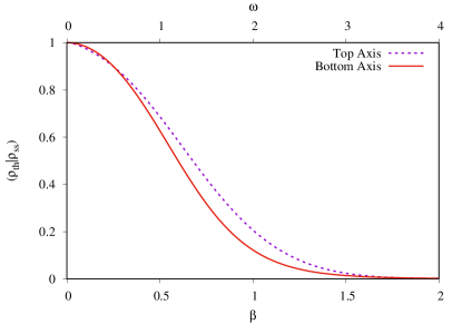
Figure 2: Overlap between the stationary- and thermodynamic-states in a system of size $N=10$. Both states have been normalized in their respective vector spaces in order to make the maximum possible overlap equal to one. The numerical values employed can be consulted in the main text. Bottom Axis: Overlap between the infinity-temperature solution of the Lindblad equation and the thermodynamic state at inverse temperature $\beta$ and fixed $\beta\mu$. Both states coincide at $\beta=0$, in accordance with the result that the stationary solution corresponds to a state of infinity temperature. Top Axis: Overlap between the thermodynamic state defined by a Hamiltonian with off-diagonal elements and the Lindblad solution with the diagonal part of the same Hamiltonian. The overlap is maximum when the off-diagonal terms vanish, showing that the stationary state obtained from the diagonal Hamiltonian is a genuine thermodynamic state.

VII Conclusions

The question of thermalization of linear Fermi systems has been addressed from the perspective of a second operational space and by making use of a reduction protocol of the quantum state. It is shown how this protocol can be implemented to encode the thermodynamic state in matrix-product representation, enabling the comparison with the stationary state of the Lindblad equation obtained also in matrix-product representation in a related work. This approach let us, on the one hand, prove two theorems providing a set of stationary solutions of the Lindblad equation, and on the other hand, establish how these solutions can in some cases be made to conform to a thermodynamic state. The first theorem characterizes systems bound to evolve toward infinity-temperature states. The second theorem provides solutions that can be fitted to thermal states only in those cases where the Hamiltonian coefficients adjust to a diagonal matrix. This behavior suggests driving mechanisms should be incorporated with at least some of their elements as non-diagonal terms, so that their effect could be differentiated from the action of the baths which, owning to the special conditions of coupling, are expected to drift the system toward thermalization. Potential application areas include, among others, the effect of an electric field on one-dimensional electrons, the simulation of laser-driving on quantum matter and the study of fluctuation-dissipation relations in linear systems.

References

- (1) T. Mori, T. Ikeda, E. Kaminishi and M. Ueda Thermalization and prethermalization in isolated quantum systems: a theoretical overview, Journal of Physics B: Atomic, Molecular and Optical Physics 51 112001 (2018).
- (2) D. Tupkary, A. Dhar, M. Kulkarni and A. Purkayastha Fundamental limitations in Lindblad descriptions of systems weakly coupled to baths, Physical Review A 105 032208 (2022). D. Tupkary, A. Dhar, M. Kulkarni and A. Purkayastha Searching for Lindbladians obeying local conservation laws and showing thermalization, arXiv:2301.02146.
- (3) I. Reichental A. Klempner Y. Kafri and D. Podolsky Thermalization in open quantum systems, Physical Review B 97:134301, (2018).
- (4) R. Nandkishore and D. Huse Many-Body Localization and Thermalization in Quantum Statistical Mechanics, Annual Review of Condensed Matter Physics 6 15 (2015).
- (5) J. Eisert, M. Friesdorf and C. Gogolin Quantum many-body systems out of equilibrium, Nature Physics, 11:124, (2015).
- (6) M. Rigol, V. Dunjko, M. Olshanii Thermalization and its mechanism for generic isolated quantum systems Nature 452 854 (2008).
- (7) N. Linden, S. Popescu, A. Short and A. Winter Quantum mechanical evolution towards thermal equilibrium Physical Review E 79 061103 (2009).
- (8) E. Ilievski Dissipation-driven integrable fermionic systems: from graded Yangians to exact nonequilibrium steady states, SciPost Physics 3:031, (2017).
- (9) T. Prosen and B. Zunkovic Exact solution of Markovian master equations for quadratic Fermi systems: thermal baths, open XY spin chains and non-equilibrium phase transition, New Journal of Physics 12:025016, (2010).
- (10) A. Rivas and S. Huelga Open Quantum Systems, SpringerBriefs in Physics (2012).
- (11) I. Vega and D. Alonso Dynamics of non-Markovian open quantum systems, 89:015001 (2017)
- (12) G. Lindblad, On the generators of quantum dynamical semigroups, 48:119, (1976).
- (13) V. Gorini, A. Kossakowski, and E. Sudarshan Completely positive dynamical semigroups of N‐level systems, Journal of Mathematical Physics 17:821 (1976)
- (14) T. Prosen Third quantization: a general method to solve master equations for quadratic open Fermi systems New Journal of Physics 10 043026 (2008).
- (15) F. Schwabl Advanced quantum mechanics, 4th edition, (Springer, Berlin, 2008).
- (16) D. Youla A normal form for a matrix under the unitary congruence group, Canadian Journal of Mathematics 13 694 (1961).
- (17) J. Reslen End-to-end correlations in the Kitaev chain, Journal of Physics Communications 2 105006 (2018).
- (18) J. Reslen Uncoupled Majorana fermions in open quantum systems: on the efficient simulation of non-equilibrium stationary states of quadratic Fermi models, Journal of Physics: Condensed Matter 32 405601 (2020).
- (19) J. Reslen Entanglement at the interplay between single- and many-bodyness, Journal of Physics A: Mathematical and Theoretical 56 155302 (2023).
- (20) G. Vidal Efficient classical simulation of slightly entangled quantum computations, Physical Review Letters 91:147901, (2003).
- (21) A Schlimgen, K. Head-Marsden, L. Sager, P. Narang and D. Mazziotti Quantum simulation of the Lindblad equation using a unitary decomposition of operators, Physical Review Research 4:023216, (2022).