Computing Marginal and Conditional Divergences between Decomposable Models with Applications

Abstract

The ability to compute the exact divergence between two high-dimensional distributions is useful in many applications but doing so naively is intractable. Computing the alpha-beta divergence—a family of divergences that includes the Kullback-Leibler divergence and Hellinger distance—between the joint distribution of two decomposable models, i.e chordal Markov networks, can be done in time exponential in the treewidth of these models. However, reducing the dissimilarity between two high-dimensional objects to a single scalar value can be uninformative. Furthermore, in applications such as supervised learning, the divergence over a conditional distribution might be of more interest. Therefore, we propose an approach to compute the exact alpha-beta divergence between any marginal or conditional distribution of two decomposable models. Doing so tractably is non-trivial as we need to decompose the divergence between these distributions and therefore, require a decomposition over the marginal and conditional distributions of these models. Consequently, we provide such a decomposition and also extend existing work to compute the marginal and conditional alpha-beta divergence between these decompositions. We then show how our method can be used to analyze distributional changes by first applying it to a benchmark image dataset. Finally, based on our framework, we propose a novel way to quantify the error in contemporary superconducting quantum computers. Code for all experiments is available at: https://lklee.dev/pub/2023-icdm/code

I Introduction

The ability to analyze and quantify the differences between two high-dimensional distributions has many applications in the fields of machine learning and data science. For instance, in the study of problems with changing distributions, i.e. concept drift [1, 2], in the detection of anomalous regions in spatio-temporal data [3, 4], and in tasks related to the retrieval, classification, and visualization of time series data [5].

There has been some previous work done on tractably computing the divergence between two high-dimensional distributions modeled by chordal , i.e.  [6]. However, reducing the differences between two distributions to just one scalar value can be quite uninformative as it does not help us better understand why the distributions are different in the first place. Specifically in high-dimensions, it is quite likely that the difference between two distributions will be largely attributable to the influence of a small proportion of the variables [2].

One way to better understand distributional changes in higher-dimensions is to measure the divergence between the marginal univariate distributions over individual variables in the two distributions [2]. However, this does not capture changes in the relationships between variables [7]. We will see further evidence on the importance of measuring changes over multiple variables at once in Section IX-A and Figure 6.

Therefore, the goal of this work is to develop a method for computing the divergence between two over arbitrary variable subsets. Doing so tractably is non-trivial, as computing the $\alpha\beta$-divergence involves a sum over an exponential number of elements with respect to the number of variables in the distributions. Therefore we need a “decomposition” of the sum in the $\alpha\beta$-divergence into a product of smaller—more tractable—sums. As we will see later on, this will require a decomposition over any marginal distribution of a into product of smaller marginal distributions as well. An example of such a decomposition can be found in Figure 1.

Figure 1: Example of decomposing the marginal distribution of a into a product of maximal clique probabilities of a new . Doing so for the general case is one of our main contributions. More details in Section VI.

To this end, we will develop the tools needed to find such a decomposition and also show that these tools can also be used to develop a method for computing the $\alpha\beta$-divergence between conditional distributions of as well. More generally, our method can be used to compute any functional that can be expressed as a linear combination of the Functional $\mathcal{F}$ in Definition 3, between any marginal or conditional distributions of 2 . In fact, it is the properties of $\mathcal{F}$, and the $\alpha\beta$-divergence being a linear combination of $\mathcal{F}$ for most values of $\alpha$ and $\beta$, that allows for the decomposition of the $\alpha\beta$-divergence over any distributions between two .

In order to underpin the relevance of our work, we provide a completely novel error analysis of real-world quantum computing devices, based on our methodology. It allows us to gain insights into the specific errors of (subsets of) qubits, which is of utmost importance for practical quantum computing.

II Related Work

There is not much previous work on computing the marginal or conditional divergences between probabilistic graphical models in general, let alone the marginal and conditional $\alpha\beta$-divergence. That said, the idea of isolating distributional changes to some subspace of the distribution is not new. For instance, [8] employed multiple base learners, each trained over a random subset of variables. When a change occurs, this approach can either update the affected learners or reduce how much they will weigh in on the final output of the ensemble. In [9], the authors create an ensemble of AESAKNNS models [10]—a model already capable of handling distributional change on its own—on different subsets of variables and samples. Furthermore, unlike [8], they vary the size of the variable subsets for model training as well, and can dynamically change it over time.

In order to explicitly detect subspaces where distributional changes occur, [11] compute a statistic between the subspace of two samples, called the local drift degree, which follows the normal distribution when both samples follow the same distribution. More recently, [12] propose their own statistic, based on the Kullback-Leibler divergence, for detecting changes in the distribution over the covariate and class variables, as well as conditional distributions between them.

III Background and Notation

For any set of $n$ random variables, $\bm{X}=\{X_{1},\ldots,X_{n}\}$, let $\mathcal{X}_{\bm{X}}=\mathcal{X}_{X_{1}}\times\ldots\times\mathcal{X}_{X_{n}}$ be the domain of $\bm{X}$, i.e. the set of values that $\bm{X}$ can take, and $\bm{x}\in\mathcal{X}_{\bm{X}}$ be one of these values. Additionally, for some subset of variables $\bm{Z}\subseteq\bm{X}$, let $\bar{\bm{Z}}$ be the set of variables in $\bm{X}$ not in $\bm{Z}$, $\bar{\bm{Z}}=\bm{X}\setminus\bm{Z}$.

III-A Statistical Divergences

A divergence is a measure of the “difference” between two probability distributions. More formally, a divergence is a functional with the following properties:

Definition 1 (Divergence)

Suppose $P$ is the set of probability distributions with the same support. A divergence, $D$, is the function $D(\cdot\ ||\ \cdot)\mathrel{\mathop{\mathchar 58\relax}}P\times P\rightarrow\mathbb{R}$ such that $\forall\mathbb{P},\mathbb{Q}\in S\mathrel{\mathop{\mathchar 58\relax}}D(\mathbb{P}\ ||\ \mathbb{Q})\geq 0$ and $\mathbb{P}=\mathbb{Q}\Leftrightarrow D(\mathbb{P}\ ||\ \mathbb{Q})=0$ .

Some popular divergences include the Kullback-Leibler (KL) divergence [14], the Hellinger distance [15], and the Itakura-Saito (IS) divergence [16, 17]. Furthermore, these aforementioned divergences can be expressed by a more general family of divergences, known as the $\alpha\beta$-divergence.

Definition 2 ($\alpha\beta$-divergence [18])

The $\alpha\beta$-divergence, $D_{\textit{AB}}$, between two positive measures $\mathbb{P}$ and $\mathbb{Q}$ is defined as

$$D_{\textit{AB}}^{\alpha,\beta}(\mathbb{P},\mathbb{Q})=\sum_{\bm{x}\in\mathcal{X}}d_{\textit{AB}}^{\alpha,\beta}\big{(}\mathbb{P}(\bm{x}),\mathbb{Q}(\bm{x})\big{)}\;,$$ (1)

where $\alpha$ and $\beta$ are parameters, and

$$d_{\textit{AB}}^{(\alpha,\beta)}(\mathbb{P}(\bm{x}),\mathbb{Q}(\bm{x}))$$ (2)

$$=\begin{cases}\frac{-1}{\alpha\beta}\left(\mathbb{P}(\bm{x})^{\alpha}\mathbb{Q}(\bm{x})^{\beta}-\frac{\alpha\mathbb{P}(\bm{x})^{\alpha+\beta}}{\alpha+\beta}-\frac{\beta\mathbb{Q}(\bm{x})^{\alpha+\beta}}{\alpha+\beta}\right),&\hfill\genfrac{}{}{0.0pt}{}{\hfil\hfill\alpha,\beta\neq 0}{\hfill\alpha+\beta\neq 0}\\ \frac{1}{\alpha^{2}}\left(\mathbb{P}(\bm{x})^{\alpha}\log\frac{\mathbb{P}(\bm{x})^{\alpha}}{\mathbb{Q}(\bm{x})^{\alpha}}-\mathbb{P}(\bm{x})^{\alpha}+\mathbb{Q}(\bm{x})^{\alpha}\right),&\hfill\genfrac{}{}{0.0pt}{}{\hfil\alpha\neq 0}{\hfill\beta=0}\\ \frac{1}{\alpha^{2}}\left(\log\frac{\mathbb{Q}(\bm{x})^{\alpha}}{\mathbb{P}(\bm{x})^{\alpha}}+\left(\frac{\mathbb{Q}(\bm{x})^{\alpha}}{\mathbb{P}(\bm{x})^{\alpha}}\right)^{-1}-1\right),&\hfill\genfrac{}{}{0.0pt}{}{\hfil\alpha=-\beta}{\hfill\alpha\neq 0}\\ \frac{1}{\beta^{2}}\left(\mathbb{Q}(\bm{x})^{\beta}\log\frac{\mathbb{Q}(\bm{x})^{\beta}}{\mathbb{P}(\bm{x})^{\beta}}-\mathbb{Q}(\bm{x})^{\beta}+\mathbb{P}(\bm{x})^{\beta}\right),&\hfill\genfrac{}{}{0.0pt}{}{\hfil\alpha=0}{\hfill\beta\neq 0}\\ \frac{1}{2}(\log\mathbb{P}(\bm{x})-\log\mathbb{Q}(\bm{x}))^{2},&\hfill\alpha,\beta=0\;.\end{cases}$$

To make subsequent developments easier, the $\alpha\beta$-divergence, when either $\alpha$ or $\beta$ is $0$, can be expressed in terms of a linear combination of the functional $\mathcal{F}$ in Definition 3 [6].

Definition 3 ($\mathcal{F}$ Functional)

For any function $L$ with the property $L\left(\prod_{x}x\right)=\sum_{x}L(x)$, and functionals $f\in\{g,h,g^{*},h^{*}\}$ with the property that $f\bigl{[}\prod_{\bm{Z}\in\mathcal{A}}P_{\bm{Z}}\bigr{]}=\prod_{\bm{Z}\in\mathcal{A}}f\bigl{[}P_{\bm{Z}}\bigr{]}$, where $\mathcal{A}\subset\mathcal{P}(\bm{X})$ and $P_{\bm{X}}=\prod_{\bm{Z}\in\mathcal{A}}P_{\bm{Z}}$, let:

$$\mathcal{F}(\mathbb{P},\mathbb{Q};g,h,g^{*},h^{*})$$

$$=\sum_{\bm{x}\in\mathcal{X}}g\big{[}\mathbb{P}\big{]}(\bm{x})\cdot h\big{[}\mathbb{Q}\big{]}(\bm{x})\cdot L\Bigl{(}g^{*}[\mathbb{P}](\bm{x})\cdot h^{*}[\mathbb{Q}](\bm{x})\Bigr{)}$$

Therefore, the $\alpha\beta$-divergence can be expressed as follows:

$$\begin{aligned} &D_{\textit{AB}}^{\alpha,\beta}(\mathbb{P},\mathbb{Q})\\ &=\begin{cases}\sum_{\bm{x}\in\mathcal{X}}\frac{1}{2}\left(\log\mathbb{P}(\bm{x})-\log\mathbb{Q}(\bm{x})\right)^{2},&\alpha,\beta=0\\ \sum_{i}c_{i}\mathcal{F}(\mathbb{P},\mathbb{Q};g_{i},h_{i},g^{*}_{i},h^{*}_{i}),&\text{otherwise}\end{cases}\end{aligned}$$ (3)

which is more terse compared to 2.

So far we have discussed divergences between joint distributions, but computing these divergences between two marginal distributions, $\mathbb{P}_{\bm{Z}}$ and $\mathbb{Q}_{\bm{Z}}$, instead, is similar as we can just plug these marginal distributions into any divergence directly.

Unfortunately, defining the divergence between two conditional distributions, $\mathbb{P}_{\bm{Y}\mid\bm{Z}}$ and $\mathbb{Q}_{\bm{Y}\mid\bm{Z}}$, is not as straightforward as they are comprised of multiple distributions over $\bm{Y}$, one of each value of $\bm{z}\in\mathcal{Z}$. There is however a “natural” definition for the conditional KL-divergence as the two natural approaches to define it, lead to the same result [19]:

$$D(\mathbb{P}_{\bm{Y}\mid\bm{Z}}\mid\mid\mathbb{Q}_{\bm{Y}\mid\bm{Z}}\mid\mathbb{P}_{\bm{Z}}) \mathrel{\mathop{\mathchar 58\relax}}=D(\mathbb{P}_{\bm{Y}\mid\bm{Z}}\mathbb{P}_{\bm{Z}}\mid\mid\mathbb{Q}_{\bm{Y}\mid\bm{Z}}\mathbb{P}_{\bm{Z}})$$ (4)

$$\mathrel{\mathop{\mathchar 58\relax}}=\mathbb{E}_{\bm{Z}\sim\mathbb{P}}\left[D(\mathbb{P}_{\bm{Y}|\bm{Z}}\mid\mid\mathbb{Q}_{\bm{Y}\mid\bm{Z}})\right]$$ (5)

Unfortunately, this equivalence is unique to the KL-divergence. For defining other conditional divergences, previous approaches have either exclusively taken the definition in 4 [20, 21, 19] or 5 [22, 23, 24]. For our purposes, we will use the definition in 5 which involves taking the expectation of $D(\mathbb{P}_{\bm{Y}\mid\bm{z}},\mathbb{Q}_{\bm{Y}\mid\bm{z}})$ with respect to $\mathbb{P}_{\bm{Z}}$.

Definition 4 (Conditional Divergence)

$$D(\mathbb{P}_{\bm{Y}\mid\bm{Z}}\mid\mid\mathbb{Q}_{\bm{Y}\mid\bm{Z}}) =\sum_{\bm{z}\in\mathcal{Z}}\mathbb{P}_{\bm{Z}}(\bm{z})D(\mathbb{P}_{\bm{Y}|\bm{z}}\mid\mid\mathbb{Q}_{\bm{Y}\mid\bm{z}})$$

III-B Graphical Models

An undirected graph, $\mathcal{G}=(V(\mathcal{G}),E(\mathcal{G}))$, consists of $n=\mathinner{\!\left\lvert V(\mathcal{G})\right\rvert}$ vertices, and edges $(u,v)\in E(\mathcal{G})$. When a subset of vertices, $\mathcal{C}\subseteq V(\mathcal{G})$, are fully connected, they form a clique. Furthermore, let $\bm{\mathcal{C}}(\mathcal{G})$ denote the set of all maximal cliques in $\mathcal{G}$, where a maximal clique is a clique that is not contained in any other clique.

III-B1 Markov Network (MN)

By associating each vertex in $\mathcal{G}$ to a random variable, $\bm{X}=\{X_{v}\mid v\in V(\mathcal{G})\}$, the graph $\mathcal{G}$ will encode a set of conditional independencies between the variables $\bm{X}$ [25]. For some probability distribution $\mathbb{P}$ over the variables $\bm{X}$, $\mathbb{P}$ is strictly positive and follows the conditional independencies in $\mathcal{G}$ if and only if it is a Gibbs distribution of the form [26]: $\mathbb{P}_{\bm{X}}(\bm{x})=\frac{1}{Z}\prod_{\mathcal{C}\in\bm{\mathcal{C}}(\mathcal{G})}\psi_{\mathcal{C}}(\bm{x}_{\mathcal{C}})$, where $Z$ is a normalizing constant, $Z=\sum_{\bm{x}\in\mathcal{X}}\prod_{\mathcal{C}\in\bm{\mathcal{C}}(\mathcal{G})}\psi_{\mathcal{C}}(\bm{x}_{\mathcal{C}})$, and $\psi_{\mathcal{C}}$ are positive factors over the domain of each maximal clique, $\psi_{\mathcal{C}}\mathrel{\mathop{\mathchar 58\relax}}\mathcal{X}_{\mathcal{C}}\to\mathbb{R}$. We denote such a with the notation $\mathcal{M}=(\mathcal{G},\Psi)$, where $\Psi=\{\psi_{\mathcal{C}}\mid\mathcal{C}\in\bm{\mathcal{C}}(\mathcal{G})\}$. Markov networks are also known as Markov random fields.

III-B2 Belief Propagation

Unfortunately, computing $Z$ directly is intractable due to the sum growing exponentially with respect to $\mathinner{\!\left\lvert\bm{X}\right\rvert}$. However, by finding a chordal graph $\mathcal{H}$ that is strictly larger than $\mathcal{G}$, we can use an algorithm known as belief propagation on the clique tree of $\mathcal{H}$ with initial factors $\Psi$, to compute not only $Z$, but also the marginal distributions of $\mathbb{P}$ over each $\mathcal{C}\in\bm{\mathcal{C}}(\mathcal{H})$. The complexity of belief propagation is $\mathcal{O}(2^{\omega(\mathcal{H})})$, where $\omega$ is the treewidth of $\mathcal{H}$, i.e. the size of the largest maximal clique in $\mathcal{H}$ minus one.

III-B3 Decomposable Model (DM)

When a has a chordal graph structure, it also has a closed form joint distribution:

$$\mathbb{P}_{\mathcal{G}}(\bm{x})=\frac{\prod_{\mathcal{C}\in\bm{\mathcal{C}}(\mathcal{G})}\mathbb{P}_{\mathcal{C}}(\bm{x}_{\mathcal{C}})}{\prod_{\mathcal{S}\in\bm{\mathcal{S}}(\mathcal{G})}\mathbb{P}_{\mathcal{S}}(\bm{x}_{\mathcal{S}})}=\prod_{\mathcal{C}\in\bm{\mathcal{C}}(\mathcal{G})}\mathbb{P}^{\mathcal{T}}_{\mathcal{C}}(\bm{x}_{\mathcal{C}})$$ (6)

where $\bm{\mathcal{S}}(\mathcal{G})$ are the sets of variables between each adjacent maximal clique in the clique tree of $\mathcal{G}$, and $\mathbb{P}^{\mathcal{T}}_{\mathcal{C}}$ is a over clique $\mathcal{C}$.

For clarity of exposition, we will only use to refer to chordal with the in 6 as factors.

IV Previous Work: Computing Joint Divergence

It has been shown [6] that the complexity of computing the $\alpha\beta$-divergence between decomposable models $\mathbb{P}_{\mathcal{G}_{\mathbb{P}}}$ and $\mathbb{Q}_{\mathcal{G}_{\mathbb{Q}}}$ is generally, in the worst case, exponential to the treewidth of the computation graph $\mathcal{U}(\mathcal{G}_{\mathbb{P}},\mathcal{G}_{\mathbb{Q}})$, as defined in Definition 5.

Definition 5 (Computation graph, $\mathcal{U}$)

Let $\mathcal{G}_{(1)}$ and $\mathcal{G}_{(2)}$ be two chordal graphs. Then denote $\mathcal{U}(\mathcal{G}_{(1)},\mathcal{G}_{(2)})$ to be a chordal graph that contains all the vertices and edges in $\mathcal{G}_{(1)}$ and $\mathcal{G}_{(2)}$. We call such a graph, the computation graph of $\mathcal{G}_{(1)}$ and $\mathcal{G}_{(2)}$.

Specifically, when $\alpha,\beta=0$, the joint distributions of $\mathbb{P}_{\mathcal{G}_{\mathbb{P}}}$ and $\mathbb{Q}_{\mathcal{G}_{\mathbb{Q}}}$ immediately decomposes the log term in the $\alpha\beta$-divergence for this case, allowing for a complexity that is exponential to the maximum treewidth between the 2 .

On the other hand, when either $\alpha$ or $\beta$ are non-zero, the decomposition of the functional $\mathcal{F}$ from Definition 3, and therefore the $\alpha\beta$-divergence in this case, is not as straightforward. Substituting the joint distribution of $\mathbb{P}_{\mathcal{G}_{\mathbb{P}}}$ and $\mathbb{Q}_{\mathcal{G}_{\mathbb{Q}}}$ into $\mathcal{F}$ eventually results in the following equation:

$$\begin{aligned} \mathcal{F}({\mathbb{P}},&{\mathbb{Q}}\;;\;g,h,g^{*},h^{*})\\ =&\sum_{\mathcal{C}\in\bm{\mathcal{C}}(\mathcal{G}_{\mathbb{P}})}\sum_{\bm{x}_{\mathcal{C}}\in\mathcal{X}_{\mathcal{C}}}L\left(g^{*}\left[\mathbb{P}_{\mathcal{C}}^{\mathcal{T}}\right](\bm{x}_{\mathcal{C}})\right)\textit{SP}_{\mathcal{C}}(\bm{x}_{\mathcal{C}})+\\ &\sum_{\mathcal{C}\in\bm{\mathcal{C}}(\mathcal{G}_{\mathbb{Q}})}\sum_{\bm{x}_{\mathcal{C}}\in\mathcal{X}_{\mathcal{C}}}L\left(h^{*}\left[\mathbb{Q}_{\mathcal{C}}^{\mathcal{T}}\right](\bm{x}_{\mathcal{C}})\right)\textit{SP}_{\mathcal{C}}(\bm{x}_{\mathcal{C}})\end{aligned}$$ (7)

where:

$$\textit{SP}_{\mathcal{C}}(\bm{x}_{\mathcal{C}})$$ (8)

$$=\sum_{\bm{x}\in\mathcal{X}_{X-\mathcal{C}}}\left[\prod_{\mathcal{C}\in\bm{\mathcal{C}}_{\mathbb{P}}}g\left[\mathbb{P}_{\mathcal{C}}^{\mathcal{T}}\right](\bm{x}_{\mathcal{C}},\bm{x})\right]\left[\prod_{\mathcal{C}\in\bm{\mathcal{C}}_{\mathbb{Q}}}h\left[\mathbb{Q}_{\mathcal{C}}^{\mathcal{T}}\right](\bm{x}_{\mathcal{C}},\bm{x})\right]$$

Therefore, computing $\mathcal{F}$ between two decomposable models relies on the ability to obtain the sum-product $\textit{SP}_{\mathcal{C}}$, from 8, for all maximal cliques, $\mathcal{C}$, in the computation graph $\mathcal{U}(\mathbb{P}_{\mathcal{G}_{\mathbb{P}}},\mathbb{Q}_{\mathcal{G}_{\mathbb{Q}}})$. These sum-products can then be further marginalized to obtain sum-products over maximal cliques of $\mathcal{G}_{\mathbb{P}}$ and $\mathcal{G}_{\mathbb{Q}}$ in 7. Specifically, [6] obtained these sum-products using belief propagation on the junction tree of $\mathcal{U}(\mathbb{P}_{\mathcal{G}_{\mathbb{P}}},\mathbb{Q}_{\mathcal{G}_{\mathbb{Q}}})$, with factors $\{g[\mathbb{P}_{\mathcal{C}}^{\mathcal{T}}]\mid\mathcal{C}\in\bm{\mathcal{C}}(\mathcal{G}_{\mathbb{P}})\}\cup\{h[\mathbb{Q}_{\mathcal{C}}^{\mathcal{T}}]\mid\mathcal{C}\in\bm{\mathcal{C}}(\mathcal{G}_{\mathbb{Q}})\}$.

V s (comps)

For the purposes of developing the methods in this paper, we will further abstract and generalize the problem of obtaining $\textit{SP}_{\mathcal{C}}$ for all $\mathcal{C}$ in $\bm{\mathcal{C}}(\mathcal{H})$ as a problem of obtaining the sum-products over two sets of factors, $\Phi_{(1)}$ and $\Phi_{(2)}$, defined over the maximal cliques over two chordal graphs, $\mathcal{G}_{(1)}$ and $\mathcal{G}_{(2)}$, respectively.

$$\forall\mathcal{C}\in\bm{\mathcal{C}}(\mathcal{H})\mathrel{\mathop{\mathchar 58\relax}}\textit{SP}_{\mathcal{C}}(\bm{x}_{\mathcal{C}})=\sum_{\bm{x}\in\mathcal{X}_{\bm{X}-\mathcal{C}}}\prod_{\phi\in\Phi_{(1)}\cup\Phi_{(2)}}\phi\left(\bm{x}_{\mathcal{C}},\bm{x}\right)$$ (9)

We can then further abstract the problem by observing that $\textit{SP}_{\mathcal{C}}$ can be seen as a sum-product over the factors of a new chordal graph constructed by merging the chordal $\mathcal{M}_{(1)}=(\mathcal{G}_{(1)},\Phi_{(1)})$ and $\mathcal{M}_{(2)}=(\mathcal{G}_{(2)},\Phi_{(2)})$ by taking their product according to Definition 6.

Definition 6 (Product of Markov netowrks)

Let $\mathcal{M}_{(1)}=(\mathcal{G}_{(1)},\Phi_{(1)})$ and $\mathcal{M}_{(2)}=(\mathcal{G}_{(2)},\Phi_{(2)})$ be two . Then, taking the product of $\mathcal{M}_{(1)}$ and $\mathcal{M}_{(2)}$, $\mathcal{M}_{(1)}\circ\mathcal{M}_{(2)}$, involves:

1. first obtaining the chordal graph $\mathcal{H}=\mathcal{U}(\mathcal{G}_{(1)},\mathcal{G}_{(2)})$,

2. then creating the factor set $\Psi=\Phi_{(1)}\cup\Phi_{(2)}$,

resulting in a new chordal , $\mathcal{M}_{\mathcal{H}}=(\mathcal{H},\Psi)$.

Once $\mathcal{M}_{\mathcal{H}}$ is obtained, like [6] we can then obtain $\forall\mathcal{C}\in\bm{\mathcal{C}}(\mathcal{H})\>\mathrel{\mathop{\mathchar 58\relax}}\>\textit{SP}_{\mathcal{C}}$ using belief propagation on the clique tree of $\mathcal{M}_{\mathcal{H}}$ with initial factors $\Psi$. However, in order to aid future developments, we shall further extend this result to obtain the sum-products over $m$ different factor sets, and not just two.

Lemma 1 ()

Let $\mathcal{M}_{(1)}=(\mathcal{G}_{(1)},\Phi_{(1)})$, $\ldots$ , $\mathcal{M}_{(m)}=(\mathcal{G}_{(m)},\Phi_{(m)})$ be $m$ , possibly defined over different sets of variables. Then, using the notion of products between from Definition 6, we can obtain the following sum-products:

$$\forall\mathcal{C}\in\bm{\mathcal{C}}(\mathcal{H})\>\mathrel{\mathop{\mathchar 58\relax}}\>\textit{SP}_{\mathcal{C}}(\bm{x}_{\mathcal{C}})=\sum_{\bm{x}\in\mathcal{X}_{\bm{X}-\mathcal{C}}}\prod_{\phi\in\bigcup_{i=1}^{m}\Phi_{(i)}}\phi\left(\bm{x}_{\mathcal{C}},\bm{x}\right)$$ (10)

by carrying out belief propagation on the junction tree of $\mathcal{U}\bigl{(}\mathcal{G}_{(1)},\ldots,\mathcal{G}_{(m)}\bigr{)}$ using the set of initial factors $\bigcup_{i=1}^{m}\Phi_{(i)}$.

Proof 1

Using Definition 6, we can first take the product of the $m$ given to obtain the chordal $\mathcal{M}_{\mathcal{H}}=(\mathcal{H},\Psi)$: $\mathcal{M}_{\mathcal{H}}=\mathcal{M}_{(1)}\circ\ldots\circ\mathcal{M}_{(m)}$ and $\Psi=\bigcup_{i=1}^{m}\Phi_{(i)}$. Then, recall that carrying out belief propagation on the junction tree of $\mathcal{M}_{\mathcal{H}}$ will result in the following beliefs over the maximal cliques of $\mathcal{H}$ [27, Corollary 10.2]:

$$\forall\mathcal{C}\in\bm{\mathcal{C}}(\mathcal{H})\>\mathrel{\mathop{\mathchar 58\relax}}\>\beta_{\mathcal{C}}(\bm{x}_{\mathcal{C}})=\sum_{\bm{x}\in\mathcal{X}_{\bm{X}-\mathcal{C}}}\prod_{\psi\in\Psi}\psi(\bm{x},\bm{x}_{\mathcal{C}})$$ (11)

which is directly equivalent to the sum-products in 10 since $\Psi=\bigcup_{i=1}^{m}\Phi_{(i)}$.

VI Marginal Divergence

The marginal distribution over the set of variables $\bm{Z}$ for a given decomposable model $\mathbb{P}_{\mathcal{G}_{\mathbb{P}}}$ can be obtained by summing over the domain of the variables not in $\bm{Z}$, $\bar{\bm{Z}}=\bm{X}\setminus\bm{Z}$.

$$\mathbb{P}_{\bm{Z}}(\bm{z})=\sum_{\bar{\bm{z}}\in\bar{\mathcal{Z}}}\mathbb{P}_{\bm{x}}(\bar{\bm{z}},\bm{z})=\sum_{\bar{\bm{z}}\in\bar{\mathcal{Z}}}\prod_{\mathcal{C}\in\bm{\mathcal{C}}(\mathcal{G}_{\mathbb{P}})}\mathbb{P}^{\mathcal{T}}_{\mathcal{C}}(\bar{\bm{z}},\bm{z})$$ (12)

However, in order to decompose the $\alpha\beta$-divergence between marginal distributions of two , we need to find a factorization of the sum over $\bar{\mathcal{Z}}$ in these marginal distributions.

VI-A Factorizing the marginal distribution of a

Factorizing the marginal distribution in 12 will require grouping together , and therefore maximal cliques of $\mathbb{P}_{\mathcal{G}_{\mathbb{P}}}$, that share any variables in the set of variables to sum out, $\bar{\bm{Z}}$. We shall call such a grouping of maximal cliques in $\mathcal{G}_{\mathbb{P}}$, an $\bm{\mathcal{N}}$-partition of $\mathcal{G}_{\mathbb{P}}$. See Figure 2a for an example of such an $\bm{\mathcal{N}}$-partition.

(a) Clique tree of a chordal graph.

(b) $\Gamma(\bm{Z},\bm{\mathcal{N}}_{\mathbb{P},\bm{Z}})$

Figure 2: An $\bm{\mathcal{N}}$-partition over a clique tree for removing the variables striked-out, and its respective $\bm{\mathcal{N}}$-graph.

Definition 7 ($\bm{\mathcal{N}}$-partition)

For any chordal graph $\mathcal{G}_{\mathbb{P}}$ and marginal variables $\bm{Z}$, with $\bar{\bm{Z}}=\bm{X}\setminus\bm{Z}$, an $\bm{\mathcal{N}}$-partition of $\mathcal{G}_{\mathbb{P}}$, $\bm{\mathcal{N}}_{\mathbb{P},\bm{Z}}$, is a set of vertex sets, $\forall N\in\bm{\mathcal{N}}_{\mathbb{P},\bm{Z}}\mathrel{\mathop{\mathchar 58\relax}}N\subset V(\mathcal{G}_{\mathbb{P}})$, with the following properties:

1. $\{\bm{\mathcal{C}}(\mathcal{G}_{\mathbb{P}}(N))\mid N\in\bm{\mathcal{N}}_{\mathbb{P},\bm{Z}}\}$ is a partition of the maximal cliques of $\mathcal{G}_{\mathbb{P}}$,

2. $\{\bar{\bm{Z}}\cap\bm{X}_{N}\mid N\in\bm{\mathcal{N}}_{\mathbb{P},\bm{Z}},\bar{\bm{Z}}\cap\bm{X}_{N}\neq\emptyset\}$ is a partition of $\bar{\bm{Z}}$,

One way to find an $\bm{\mathcal{N}}$-partition of $\mathcal{G}_{\mathbb{P}}$ is to group maximal cliques of $\mathcal{G}_{\mathbb{P}}$ that share any variables that are also in $\bar{\bm{Z}}$.

Corollary 1 (Decomposition of Marginal Distribution)

Using $\bm{\mathcal{N}}$-partitions from Definition 7, the marginal distribution over variables $\bm{Z}$ of a decomposable model $\mathbb{P}_{\mathcal{G}_{\mathbb{P}}}$ can be factorized over the variables sets in $\bm{\mathcal{N}}_{\mathbb{P},\bm{Z}}$:

$$\begin{aligned} \mathbb{P}_{\bm{Z}}(\bm{z})&=\prod_{N\in\bm{\mathcal{N}}_{\mathbb{P},\bm{Z}}}\sum_{\bar{\bm{z}}\in\bar{\mathcal{Z}}_{N}}\prod_{\mathcal{C}\in\bm{\mathcal{C}}(\mathcal{G}_{\mathbb{P}}(N))}\mathbb{P}^{\mathcal{T}}_{\mathcal{C}}(\bm{z}_{\mathcal{C}},\bar{\bm{z}}_{\mathcal{C}})\\ &=\prod_{N\in\bm{\mathcal{N}}_{\mathbb{P},\bm{Z}}}\varphi_{N\cap\bm{Z}}[\mathbb{P}](\bm{z}_{N})\end{aligned}$$ (13)

where for ease of notation, we use $\varphi_{\bm{\mathcal{N}}\cap{\bm{Z}}}$ as shorthand for marginalizing factors in $N$ to remove any variables in $\bar{\bm{Z}}$. See Definition 8 for a full definition of $\varphi_{\bm{\mathcal{N}}\cap{\bm{Z}}}$.

Definition 8 ($(N\cap\bm{Z})$-Marginalised Factor, $\varphi_{N\cap\bm{Z}}$)

Through a slight abuse of notation, let $N\cap\bm{Z}\mathrel{\mathop{\mathchar 58\relax}}=N\cap V(\bm{Z})$. Then we define the $(N\cap\bm{Z})$-marginalized factor as such:

$$\varphi_{N\cap\bm{Z}}[\mathbb{P}](\bm{z}_{N})\mathrel{\mathop{\mathchar 58\relax}}=\sum_{\bar{\bm{z}}\in\bar{\mathcal{Z}}_{N}}\prod_{\mathcal{C}\in\bm{\mathcal{C}}(\mathcal{G}_{\mathbb{P}}(N))}\mathbb{P}^{\mathcal{T}}_{\mathcal{C}}(\bm{z}_{\mathcal{C}},\bar{\bm{z}}_{\mathcal{C}})$$ (14)

Note that it is possible for $\varphi_{N\cap\bm{Z}}$ to be defined over the empty set when $N\cap\bm{Z}=\{\}\Leftrightarrow\bm{X}_{N}\subseteq\bar{\bm{Z}}$. In such situations, $\varphi_{N\cap\bm{Z}}$ is just a scalar factor, i.e. a number in $\mathbb{R}$. For ease of exposition, we shall also define a function $\bm{\varphi}$ that returns a set of $(N\cap\bm{Z})$-marginalized factors given an $\bm{\mathcal{N}}$-partition $\bm{\mathcal{N}}_{\mathbb{P},\bm{Z}}$:

$$\bm{\varphi}(\bm{\mathcal{N}}_{\mathbb{P},\bm{Z}})\mathrel{\mathop{\mathchar 58\relax}}=\Bigl{\{}\varphi_{N\cap\bm{Z}}[\mathbb{P}]\Bigm{|}N\in\bm{\mathcal{N}}_{\mathbb{P},\bm{Z}}\Bigr{\}}$$ (15)

To summarize, we finally now have factorization of $\mathbb{P}_{\bm{Z}}$ in terms of a product of factors defined over each set in the partition $\bm{\mathcal{N}}_{\mathbb{P},\bm{Z}}$.

$$\mathbb{P}_{\bm{Z}}(\bm{z}) =\prod_{N\in\bm{\mathcal{N}}_{\mathbb{P},\bm{Z}}}\varphi_{N\cap\bm{Z}}[\mathbb{P}](\bm{z}_{N})$$ (16)

These set of factors imply an new graph structure where an edge exists between any two vertices in $\bm{Z}$ if there is any set in $\bm{\mathcal{N}}_{\mathbb{P},\bm{Z}}$ that contains both vertices together. We will call these new graphs based on the sets in an $\bm{\mathcal{N}}$-partition, $\bm{\mathcal{N}}$-graphs. See Figures 2a and 2b for an example of an $\bm{\mathcal{N}}$-partition and its respective $\bm{\mathcal{N}}$-graph.

Definition 9 (Sets-to-Cliques graph constuctor, $\kappa(\bm{\mathcal{N}})$)

Let $\bm{\mathcal{N}}$ be a set of vertex-sets. Then $\kappa$ is a graph constructor that creates a graph $\mathcal{K}$ with the following vertices and edges:

$$V(\mathcal{K})=\bigcup_{N\in\bm{\mathcal{N}}}N$$

$$E(\mathcal{K})=\bigl{\{}(u,v)\bigm{|}N\in\bm{\mathcal{N}},(v,u)\in N,v\neq u\bigr{\}}$$

Therefore, the graph constructor $\kappa(\bm{\mathcal{N}})$ ensures that each vertex-set in $\bm{\mathcal{N}}$ is also as clique in the resulting graph $\mathcal{K}$.

Definition 10 ($\bm{\mathcal{N}}$-graphs, $\Gamma(\bm{\mathcal{N}}_{\mathbb{P},\bm{Z}})$)

Let $\mathcal{G}_{\mathbb{P}}$ be a chordal graph with an $\bm{\mathcal{N}}$-partition $\bm{\mathcal{N}}_{\mathbb{P},\bm{Z}}$. Then $\Gamma(\bm{\mathcal{N}}_{\mathbb{P},\bm{Z}})$ is a function that will take the graph constructed by $\kappa(\bm{\mathcal{N}}_{\mathbb{P},\bm{Z}})$ from Definition 9 and remove any vertex or edges associated with any variables in $\bar{\bm{Z}}$.

Theorem 1 (The $\bm{\mathcal{N}}$-graph created by $\Gamma$ is a chordal graph)

Let $\mathcal{G}_{\mathbb{P}}$ be a chordal graph and $\bm{Z}\subset\bm{X}$. Then the $\bm{\mathcal{N}}$-graph, $\Gamma(\bm{\mathcal{N}}_{\mathbb{P},\bm{Z}})$, is a chordal graph.

Proof 2

Constructing $\Gamma(\bm{\mathcal{N}}_{\mathbb{P},\bm{Z}})$ involves two steps: 1) merging maximal cliques in the same partition via $\kappa(\bm{\mathcal{N}}_{\mathbb{P},\bm{Z}})$, and 2) removing any vertices and edges associated with $\bar{\bm{Z}}$. We will show that the resulting graph after both steps are chordal.

• Only adjacent maximal cliques in the clique tree of $\mathcal{G}_{\mathbb{P}}$ can be in the same partition in $\bm{\mathcal{N}}_{\mathbb{P},\bm{Z}}$. Merging adjacent maximal cliques in a clique tree will result in yet another clique tree, implying the graph $\kappa(\bm{\mathcal{N}}_{\mathbb{P},\bm{Z}})$ is also chordal.

• The deletion of all vertices and edges associated with $\bar{\bm{Z}}$ is equivalent to the induced subgraph over the vertices $V(\bm{Z})$. But any induced subgraph of a chordal graph is also a chordal graph [28].

Therefore, $\Gamma(\bm{\mathcal{N}}_{\mathbb{P},\bm{Z}})$ is a chordal graph.

In conclusion, the factorization of $\mathbb{P}_{\bm{Z}}$ essentially creates a new chordal Markov network consisting of the graph $\Gamma(\bm{\mathcal{N}}_{\mathbb{P},\bm{Z}})$ and factors $\bm{\varphi}(\bm{\mathcal{N}}_{\mathbb{P},\bm{Z}})$, $\mathcal{M}_{\mathbb{P},\bm{Z}}=\bigl{(}\Gamma(\bm{\mathcal{N}}_{\mathbb{P},\bm{Z}}),\bm{\varphi}(\bm{\mathcal{N}}_{\mathbb{P},\bm{Z}})\bigr{)}$.

VI-B Computing the Marginal $\alpha\beta$-Divergence between

With this factorization of the marginal distribution of a , and even a graphical representation of these factorizations, the problem of computing the $\alpha\beta$-divergence between the marginal distributions of two becomes surprisingly straightforward as a direct equivalence can made to the problem of computing the joint divergence between two .

Recall from Section IV that when [6] tackled the problem of computing the joint divergence between $\mathbb{P}_{\mathcal{G}_{\mathbb{P}}}$ and $\mathbb{Q}_{\mathcal{G}_{\mathbb{Q}}}$, they represented the joint distribution of a as a set of defined over the maximal cliques of a chordal graph. These are fundamentally just ordinary factors over their respective variables, and [6] did not rely on any special property of these factors to compute the $\alpha\beta$-divergence between these representations of .

Thanks to the factorization from Section VI-A, we have a similar problem setup to computing the joint divergence. Specifically, problem of computing the $\alpha\beta$-divergence between the marginal distributions $\mathbb{P}_{\bm{Z}}$ and $\mathbb{Q}_{\bm{Z}}$, of $\mathbb{P}_{\mathcal{G}_{\mathbb{P}}}$ and $\mathbb{Q}_{\mathcal{G}_{\mathbb{Q}}}$ respectively, becomes a problem of computing the $\alpha\beta$-divergence between the chordal : $\mathcal{M}_{\mathbb{P},\bm{Z}}=\bigl{(}\Gamma(\bm{\mathcal{N}}_{\mathbb{P},\bm{Z}}),\bm{\varphi}(\bm{\mathcal{N}}_{\mathbb{P},\bm{Z}})\bigr{)}$ and $\mathcal{M}_{\mathbb{Q},\bm{Z}}=\bigl{(}\Gamma(\bm{\mathcal{N}}_{\mathbb{Q},\bm{Z}}),\bm{\varphi}(\bm{\mathcal{N}}_{\mathbb{Q},\bm{Z}})\bigr{)}$.

Therefore, the complexity of computing the $\alpha\beta$-divergence between factorizations of $\mathbb{P}_{\bm{Z}}$ and $\mathbb{Q}_{\bm{Z}}$ is just the complexity of the approach in [6]. However, that does not include the complexity of obtaining the factorization of $\mathbb{P}_{\bm{Z}}$ and $\mathbb{Q}_{\bm{Z}}$.

Theorem 2

The worst case complexity of obtaining the factorization from Section VI-A of $\mathbb{P}_{\bm{Z}}$ for some $\mathbb{P}_{\mathcal{G}_{\mathbb{P}}}$ is:

$$\mathcal{O}\left(|\bm{X}|\cdot 2^{|N^{*}|}\right)$$ (17)

where $N^{*}\mathrel{\mathop{\mathchar 58\relax}}=\operatorname*{arg\,max}_{N\in\bm{\mathcal{N}}_{\mathbb{P},\bm{Z}}}|N|$.

Proof 3

For any $N\in\bm{\mathcal{N}}_{\mathbb{P},\bm{Z}}$, obtaining the marginal factor $\varphi_{N\cap\bm{Z}}[\mathbb{P}]$ requires us to essentially iterate through each value $\bm{x}\in\mathcal{X}_{N}$ in the worst case, resulting in the complexity of $2^{|N|}$. This complexity is bounded by the complexity for the largest partition in $\bm{\mathcal{N}}_{\mathbb{P},\bm{Z}}$, $N^{*}\mathrel{\mathop{\mathchar 58\relax}}=\operatorname*{arg\,max}_{N\in\bm{\mathcal{N}}_{\mathbb{P},\bm{Z}}}\mathinner{\!\left\lvert N\right\rvert}$. Since we need to obtain $\varphi_{N\cap\bm{Z}}[\mathbb{P}]$ for all $N\in\bm{\mathcal{N}}_{\mathbb{P},\bm{Z}}$, and $|\bm{\mathcal{N}}_{\mathbb{P},\bm{Z}}|$ in bounded by $|\bm{X}|$, the final complexity is $\mathcal{O}\left(|\bm{X}|\cdot 2^{|N^{*}|}\right)$.

Therefore, the complexity of $D_{AB}^{(\alpha,\beta)}(\mathbb{P}_{\bm{Z}}||\mathbb{Q}_{\bm{Z}})$ is:

$$D_{AB}^{(\alpha,\beta)}(\mathbb{P}_{\bm{Z}}||\mathbb{Q}_{\bm{Z}})$$ (18)

$$\in\mathcal{O}\left(\mathinner{\!\left\lvert\bm{X}\right\rvert}\cdot 2^{|N^{*}|}\right)\cdot\begin{cases}\mathcal{O}(|\bm{X}|^{2}\cdot\omega_{\text{max}}2^{\omega_{\text{max}}+1})&\alpha,\beta=0\\ \mathcal{O}(|\bm{X}|\cdot 2^{\omega(\mathcal{H})+1})&\text{otherwise}\end{cases}$$

where $\omega_{\text{max}}=\max(\omega(\Gamma(\bm{\mathcal{N}}_{\mathbb{P},\bm{Z}})),\omega(\Gamma(\bm{\mathcal{N}}_{\mathbb{P},\bm{Z}})))$ and $\mathcal{H}=\mathcal{U}(\Gamma(\bm{\mathcal{N}}_{\mathbb{P},\bm{Z}}),\Gamma(\bm{\mathcal{N}}_{\mathbb{P},\bm{Z}}))$.

VII Conditional Divergence

We will now show that having a factorization of any marginal distribution for a allows us to compute the conditional $\alpha\beta$-divergence between two . Recall from Definition 4 the definition of the conditional $\alpha\beta$-divergence we will use, where $\bm{Z}\cup\bm{Y}\subseteq\bm{X}$, and $\bm{Z}\cap\bm{Y}=\{\}$:

$$D_{\textit{AB}}^{(\alpha,\beta)}(\mathbb{P}_{\bm{Y}\mid\bm{Z}}\mid\mid\mathbb{Q}_{\bm{Y}\mid\bm{Z}})=\sum_{\bm{z}\in\mathcal{Z}}\mathbb{P}_{\bm{Z}}(\bm{z})D_{\textit{AB}}^{(\alpha,\beta)}(\mathbb{P}_{\bm{Y}\mid\bm{z}}\mid\mid\mathbb{Q}_{\bm{Y}\mid\bm{z}})$$

where

$$\begin{aligned} &D_{\textit{AB}}^{(\alpha,\beta)}(\mathbb{P}_{\bm{Y}\mid\bm{z}}\mid\mid\mathbb{Q}_{\bm{Y}\mid\bm{z}})\\ &=\begin{cases}\sum_{\bm{y}\in\mathcal{Y}}\frac{1}{2}\left(\log\mathbb{P}_{\bm{Y}\mid\bm{z}}(\bm{y})-\log\mathbb{Q}_{\bm{Y}\mid\bm{z}}(\bm{y})\right)^{2}&\alpha,\beta=0\\ \sum_{i}c_{i}\mathcal{F}(\mathbb{P}_{\bm{Y}\mid\bm{z}},\mathbb{Q}_{\bm{Y}\mid\bm{z}};g_{i},h_{i},g^{*}_{i},h^{*}_{i})&\text{else}\end{cases}\end{aligned}$$

To assist in future developments, we shall define a notion of taking the quotient between two .

Definition 11 (Quotient of Markov netowrks)

Assume we are given 2 , $\mathcal{M}_{\bm{X}}=(\mathcal{G}_{\bm{X}},\Phi_{\bm{X}})$ and $\mathcal{M}_{\bm{Z}}=(\mathcal{G}_{\bm{Z}},\Phi_{\bm{Z}})$. Then the quotient $\mathcal{M}_{\bm{X}}/\mathcal{M}_{\bm{Z}}$ involves:

1. first finding chordal graph $\mathcal{H}=\mathcal{U}(\mathcal{G}_{\bm{X}},\mathcal{G}_{\bm{Z}})$,

2. then creating the factor set: $\Psi=\Phi_{\bm{X}}\cup\bigl{\{}1/\phi\bigm{|}\phi\in\Phi_{\bm{Z}}\bigr{\}}$

This results in the chordal $\mathcal{M}=(\mathcal{H},\Psi)$.

Lemma 2 (Sum-Quotient)

Let $\mathcal{M}_{\bm{X}}=(\mathcal{G}_{\bm{X}},\Phi_{\bm{X}})$ and $\mathcal{M}_{\bm{Z}}=(\mathcal{G}_{\bm{Z}},\Phi_{\bm{Z}})$ be where $\bm{Z}\subset\bm{X}$ and $\mathcal{M}_{\bm{Z}}$ is a marginalization of $\mathcal{M}_{\bm{X}}$. Then the Sum-Quotients:

$$\forall\mathcal{C}\in\bm{\mathcal{C}}(\mathcal{H})\>\mathrel{\mathop{\mathchar 58\relax}}\>\textit{SP}_{\mathcal{C}}(\bm{x}_{\mathcal{C}})=\sum_{\bm{x}\in\mathcal{X}_{\bm{X}-\mathcal{C}}}\frac{\prod_{\phi\in\Phi_{\bm{X}}}\phi\left(\bm{x}_{\mathcal{C}},\bm{x}\right)}{\prod_{\phi\in\Phi_{\bm{Z}}}\phi\left(\bm{z}_{\mathcal{C}},\bm{z}\right)}$$ (19)

can be obtained using belief propagation over the clique tree of the resulting from the quotient $\mathcal{M}_{\bm{X}}/\mathcal{M}_{\bm{Z}}$.

Proof 4

The proof follows the exact same argument as the proof for Lemma 1. However, since quotients are involved, we need to ensure the quotient in 19 is always defined, assuming $0/0=0$ [27, Definition 10.7]. We know that any sum, and therefore marginalization, over a product of factors that results in zero, implies that the original product of factors is zero as well. Therefore, since $\mathcal{M}_{\bm{Z}}$ is a marginalization of $\mathcal{M}_{\bm{X}}$, whenever the denominator in 19 is $0$, its numerator is as well.

Corollary 2 (Decomposition of Conditional Distribution)

Let $\bm{Z},\bm{Y}\subset\bm{X}$; $\bm{Z}\cap\bm{Y}=\emptyset$; and $\bm{W}=\bm{Y}\cup\bm{Z}$. Then the conditional distribution of a , $\mathbb{P}_{\bm{Y}\mid\bm{Z}}$, can be expressed as the quotient $\mathbb{P}_{\bm{W}}/\mathbb{P}_{\bm{Z}}$. Both $\mathbb{P}_{\bm{W}}$ and $\mathbb{P}_{\bm{Z}}$ can be expressed as the chordal $\mathcal{M}_{\bm{W}}=(\Gamma(\bm{\mathcal{N}}_{\mathbb{P},\bm{W}}),\bm{\varphi}(\bm{\mathcal{N}}_{\mathbb{P},\bm{W}}))$ and $\mathcal{M}_{\bm{Z}}=(\Gamma(\bm{\mathcal{N}}_{\mathbb{P},\bm{Z}}),\bm{\varphi}(\bm{\mathcal{N}}_{\mathbb{P},\bm{Z}}))$. The quotient $\mathcal{M}_{\bm{W}}/\mathcal{M}_{\bm{Z}}$ then results in the $\mathcal{M}_{\bm{Y}\mid\bm{Z}}^{(\mathbb{P})}=(\mathcal{H},\varphi^{c}(\bm{\mathcal{N}}_{\mathbb{P},\bm{W}},\bm{\mathcal{N}}_{\mathbb{P},\bm{Z}}))$ where:

$$\mathcal{H}=\mathcal{U}(\Gamma(\bm{\mathcal{N}}_{\mathbb{P},\bm{W}}),\Gamma(\bm{\mathcal{N}}_{\mathbb{P},\bm{Z}}))=\kappa(\bm{\mathcal{N}}_{\mathbb{P},\bm{Z}})$$

$$\varphi^{c}(\bm{\mathcal{N}}_{\mathbb{P},\bm{W}},\bm{\mathcal{N}}_{\mathbb{P},\bm{Z}})\mathrel{\mathop{\mathchar 58\relax}}=\bm{\varphi}(\bm{\mathcal{N}}_{\mathbb{P},\bm{W}})\cup\bigl{\{}1/\varphi\bigm{|}\varphi\in\bm{\varphi}(\bm{\mathcal{N}}_{\mathbb{P},\bm{Z}})\bigr{\}}$$

and the product of the factors in $\mathcal{M}_{\bm{Y}\mid\bm{Z}}^{(\mathbb{P})}$ is a decomposition of the conditional distribution $\mathbb{P}_{\bm{Y}\mid\bm{Z}}$.

With Corollary 2 we now have all the tools needed to tackle computing $D_{\textit{AB}}^{(\alpha,\beta)}(\mathbb{P}_{\bm{Y}\mid\bm{Z}}\mid\mid\mathbb{Q}_{\bm{Y}\mid\bm{Z}})$.

Theorem 3

Let $\bm{Z},\bm{Y}\subset\bm{X}$; $\bm{Z}\cap\bm{Y}=\emptyset$; and $\bm{W}=\bm{Y}\cup\bm{Z}$. The complexity of computing the conditional $\alpha\beta$-divergence between two , $\mathbb{P}_{\mathcal{G}_{\mathbb{P}}}$ and $\mathbb{Q}_{\mathcal{G}_{\mathbb{Q}}}$, $D_{\textit{AB}}^{(\alpha,\beta)}(\mathbb{P}_{\bm{Y}\mid\bm{Z}}\mid\mid\mathbb{Q}_{\bm{Y}\mid\bm{Z}})$, when either $\alpha$ or $\beta$ is $0$ is:

$$D_{\textit{AB}}^{(\alpha,\beta)}(\mathbb{P}_{\bm{Y}\mid\bm{Z}}\mid\mid\mathbb{Q}_{\bm{Y}\mid\bm{Z}})\in\mathcal{O}\left(\mathinner{\!\left\lvert\bm{X}\right\rvert}\cdot 2^{\omega(\mathcal{H})+1}\right)$$

where $\mathcal{H}=\mathcal{U}(\kappa(\bm{\mathcal{N}}_{\mathbb{P},\bm{Z}}),\kappa(\bm{\mathcal{N}}_{\mathbb{Q},\bm{Z}}))$.

Proof 5

See Appendix A.

Theorem 4

$\bm{Y}\subset\bm{X}$; $\bm{Z}\cap\bm{Y}=\emptyset$; and $\bm{W}=\bm{Y}\cup\bm{Z}$. The complexity of $D_{\textit{AB}}^{(\alpha,\beta)}(\mathbb{P}_{\bm{Y}\mid\bm{Z}}\mid\mid\mathbb{Q}_{\bm{Y}\mid\bm{Z}})$ when $\alpha,\beta=0$ is:

$$D_{\textit{AB}}^{(0,0)}(\mathbb{P}_{\bm{Y}\mid\bm{Z}}\mid\mid\mathbb{Q}_{\bm{Y}\mid\bm{Z}})\in\mathcal{O}\left(\mathinner{\!\left\lvert\bm{X}\right\rvert}^{2}\cdot 2^{\omega(\mathcal{H})+1}\right)$$

where $\mathcal{H}=\mathcal{U}(\kappa(\bm{\mathcal{N}}_{\mathbb{P},\bm{Z}}),\kappa(\bm{\mathcal{N}}_{\mathbb{Q},\bm{Z}}))$.

Proof 6

See Appendix B.

Therefore, the complexity of computing the conditional $\alpha\beta$-divergence between two in the worst case is just the complexity when both $\alpha$ and $\beta$ are $0$, as expressed in Theorem 4.

VIII Experiments with QMNIST

We demonstrate the basic functionality of our method by analyzing distributional changes within image data. Since image data is interpretable by most humans, this will allow us to verify any findings from the analysis of our method.

We consider the QMNIST dataset [29]. It was proposed as a reproducible recreation of the original MNIST dataset [30, 31], using data from the NIST Handprinted Forms and Characters Database, also known as NIST Special Database 19 [32].

An interesting fact about NIST Special Database 19 is that it consists of handwriting from both NIST employees and high school students. In QMNIST, images from NIST employees have the value $0$ and $1$ for the variable hsf, while images from students have a value of $4$. In Figure 3, by taking the mean over all the digits written by each group, we can observe that the handwriting of NIST employees tend to be more slanted compared to the handwriting of the students. The question now is, can our method pick up on these differences as well?

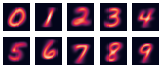
(a) NIST employees

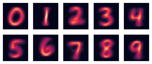
(b) High school students

Figure 3: Mean over all digits written by (a) NIST employees, and (b) high school students

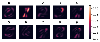
Figure 4: The marginal Hellinger distance over each pixel.

In order to test this, we need to learn 10 pairs of , one for each digit—i.e. 0, 1, etc.—with each pair containing the learnt over the 2 writer groups—NIST employees and students. Since each image has a resolution of $28\times 28$ pixels, we have $784$ pixels, and therefore $784$ variables, to learn our over. We do this by first learning the chordal graph structure for each using Chordalysis [33, 34, 35]. Specifically from which, we employ the Stepwise Multiple Testing learner [36] with a p-value threshold of $0.05$. Once we have the structure for each , we learn their parameters using pgmpy [37], specifically its BayesianEstimator parameter estimator with Dirichlet priors and a pseudo count of $1$. Once done, we now have 2 for each type of digit.

By marginalizing the learnt over each of the $28\times 28$ pixels, and computing the marginal Hellinger distance between the marginalized in each pair, we can immediately observe from Figure 4 that the digit with the most pronounced difference is $1$. Between the two writer groups, the top and bottom half of the digit $1$ changes drastically, while the middle of the digit remains relatively unchanged. This corresponds to the difference between how a regular and slanted $1$ is written.

We can also observe some clear changes to the top right and bottom half of digits $4$ and $9$, with these changes looking similar in both digits. This corresponds to the observation from Figure 3 that both digits have a similar downward stroke on the right, which changes similarly between the two writer groups. Other examples of changes observable in Figure 3 that are also highlighted by our method in Figure 4 are: the digit $0$ changing relatively more at the top and bottom left, $\{3,2,8\}$ mostly changing mostly in the top right and bottom left, and $5$ changing mostly at the top and bottom—but not as much in the middle.

However, our method seems to have picked up on more subtle changes that that a brief visual inspection of Figure 3 could have missed. For instance, although in Figure 3 it might look like digit $7$ differs the most in the downwards stroke at its bottom half, Figure 4 indicates that the area with the greatest difference for $7$ is in its top right instead.

IX Quantum Error Analysis

Our second set of experiments addresses the quantification of the effective error behavior of quantum circuits. A quantum circuit over $n$ qubits is a $2^{n}\times 2^{n}$ unitary complex matrix $C$. It acts on a quantum state $\ket{\phi}$—a $2^{n}$-dimensional, $\ell_{2}$-normalized complex vector. The computation of an $n$-qubit quantum computer with circuit $C$ can hence be written as $\ket{\psi}=C\ket{\phi}$. Denoting the $i$-th standard basis unit vector by $\bm{e}_{i}$, any quantum state can be decomposed as $\sum_{i=0}^{2^{n}-1}\alpha_{i}\bm{e}_{i}$ with $\sum_{i=0}^{2^{n}-1}|\alpha_{i}|^{2}=1$. Clearly, the $2^{n}$-dimensional output vector is never realized on a real-world quantum computer, as this would require an exponential amount of memory. Instead, a quantum computer outputs a random $n$-bit string, where the bit string that represents the standard binary encoding of the unsigned integer $i$ is sampled with probability $\mathbb{P}(i)=|(C\ket{\phi})_{i}|^{2}$, according to the Born-rule. However, due to various sources of error, samples from real-world quantum computers are generated from a (sometimes heavily) distorted distribution $\mathbb{Q}$.

In what follows, we show how to apply marginal divergences $D_{\textit{AB}}^{(\alpha,\beta)}(\mathbb{P}_{\bm{Z}}\mid\mid\mathbb{Q}_{\bm{Z}})$ for quantifying the error for specific (subsets of) qubits. To this end, we conduct two sets of experiments.

Figure 5: Quantum circuits used in our single qubit experiments.

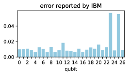
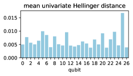
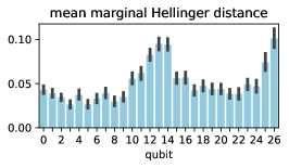
Figure 6: Left: Single qubit errors for ‘ibmq_ehningen’ as reported by IBM after we ran the experiments (June 1st, 3am). Center: Mean Hellinger distance over the two circuits used in the single qubit experiment. Right: Mean univariate marginal Hellinger distance over all 300 pairs of .

First, we consider simple single qubit circuits, shown in Figure 5. In Figure 5 a), $C$ is the identity matrix and the input state $\ket{\phi}$ is set to $\ket{0}$, i.e., the zero state. This circuit is deterministic—an exact simulation of this circuit will always output $0$. In Figure 5 b), $C=\begin{pmatrix}0&1\\ 1&0\end{pmatrix}$ is the so-called Pauli-$X$ matrix and the input state $\ket{\phi}$ is set to $\ket{0}$. An exact simulation of this circuit will always output $1$.

Nevertheless, on a real-world quantum computer, there is a small probability, that both circuits will deliver the incorrect result. Moreover, on quantum processors with more than one qubit, the error depends on the specific hardware qubit that is selected to run the circuit—each hardware qubit has its own error behavior. The precise error is typically unknown, but quantum hardware vendors deliver rough estimates of these quantities.

Here, we employ ‘ibmq_ehningen’, an IBM Falcon r5.11 superconducting quantum processing unit (QPU) with 27 qubits. The corresponding single qubit errors that IBM reports for the time we ran our experiments are provided in Figure 6 (left). Wired connections between qubits are shown in Figure 7. We run both circuits $N=10000$ times on each of the 27 qubits, resulting in a total $2\times 27\times 10000=540000$ samples for the single qubit experiment.

For the second set of experiments, we consider the quantum Fourier transform (QFT) [38]. QFT is an essential building block of many quantum algorithms, notably Shor’s algorithm for factoring and computing the discrete logarithm, as well as quantum phase estimation. We refer to [39] for an elaborate introduction to these topics.

Here, we run the QFT on $300$ uniformly random inputs on the same 27 qubit QPU as before. Each circuit is sampled $N=10000$ times, resulting in a total of $2\times 10^{6}$ samples for the QFT experiment.

For the sake of reproducibility, the circuits, data, and python scripts will be made available after acceptance of this manuscript.

IX-A Single Qubit Divergence

During transpilation, a sub-set of all available qubits is chosen to realize the logical circuit. The user can decide to consider only a specific sub-set of candidate qubits. Thus, reliable information about the effective error behavior of each qubit when used within a quantum circuit is of utmost importance.

Based on data from the single qubit experiments, we estimate $\mathbb{Q}_{i}$, that is, the probability that the $i$-th qubit takes a specific value (0 or 1). Moreover, we obtain an empirical estimate of the ground truth $\mathbb{P}_{i}$ from the exact simulated results, which allows us to compute the Hellinger distance between $\mathbb{P}$ and $\mathbb{Q}$ for each qubit. We do this for both circuits from Figure 5. The average qubit-wise Hellinger distance is reported in Figure 6 (center).

The results help us to quantify the isolated error behavior of each qubit. We see that our results qualitatively agree with the errors reported by IBM, e.g., the top-5 qubits which show the largest divergence $\{5,11,20,23,25\}$ also accumulate the largest error mass as reported by IBM. Explaining all the discrepancies is neither possible—since the exact procedure for reproducing the IBM errors in unknown—nor required. The result clearly shows that the numbers reported by IBM quantify the isolated error behavior of each qubit. We will now see that one obtains a different picture when qubits are used within a larger circuit (which is the most common use-case).

To this end, we consider the results from the QFT circuits. We learn 300 pairs of on the samples using the same methodology as in Section VIII. We then compute the marginal divergence for each qubit and report the average over all 300 QFT circuits in Figure 6 (right). As these numbers are marginals of the full joint divergence, we now quantify how each qubit behaves on average when it is part of a larger circuit.

We see that the result mostly disagrees with both, the errors reported by IBM and the single qubit divergences reported by us. First, we see that qubits 12, 13, and 14—the qubits directly in the middle of the coupling map shown in Figure 7–which are qubits that, individually, did not have much error according to both our experiments in Figure 6 (center) and the reported errors from IBM. However, it is not a coincidence that most of these high error qubits are concentrated in the middle of the circuit. Unlike in an idealized QPU, the qubits in the physical QPU we used are not all coupled with each other. Therefore, routing has to take place whenever a quantum circuit operates on pairs of qubits which are not physically connected. As a result, the states of the qubits in the middle of the circuit—qubits 12, 13, and 14—needs to be pushed around and stored in other qubits more often. This is done in order to make way for routes between qubits of opposing sides of the circuit. The more frequently these states get pushed around, the greater the chance of an error occurring, hence why these qubits in the middle exhibit the greatest amount of error. To the best of our knowledge no quantum hardware vendor reports such numbers, although they are highly important when logic qubits are transpiled to a circuit that is mapped to the actual hardware.

From Figure 6 (right), we can also observe a spike in the Hellinger distance for qubits 25 and 26. While qubit 25 is a heavy hitter in Figure 6, this does not apply for qubit 26. Moreover, qubit 26 is a “leaf” qubit (w.r.t Figure 7) and hence not used heavily for routing. Therefore, our approach reveals a type of error that is not detected by standard methods, e.g., cross-talk or three-level-system activity.

IX-B High-Order Divergence

Figure 7: The coupling map for the 27 qubit IBM Falcon r5.11 QPU

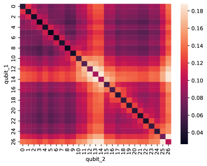
Figure 8: Mean pairwise marginal Hellinger distance over all pairs of .

We finish our analysis by investigating marginal divergence beyond single qubits. Figure 8 shows the result of computing the pairwise marginal Hellinger distance between the in each pair, taking the mean over all the pairs. The resulting heatmap is symmetrical due to Hellinger distance being a symmetric divergence. The first immediate observation is the bright bands over pairs that include qubits that already have a high univariate marginal Hellinger distance—such as qubits 12, 13, 14, 25, and 26. Another interesting observation is the bright band that occurs across the diagonal of the heatmap. We believe this is due to higher order interactions between coupled qubits, that do not necessarily exist between qubits that are multiple jumps away from each other. There are multiple causes for these higher-order interactions, ranging from unintended physical processes—such as cross-talk [40, 41]—to limitations of current QPUs—such as states being swapped between qubits solely for the purposes of routing.

These higher-order interactions are not just limited to pairwise interactions. As an example, we have discovered 70 cases where a 3-tuple of qubits, $A$, has a greater Hellinger distance than some other 3-tuple of qubits, $B$, despite the maximum Hellinger distance over all the pairwise combinations of the qubits in $A$ being less than the minimum over that of $B$. This clearly shows that our method is applicable for recovering high-order error behavior that cannot be deduced by simply investigating low-order terms.

X Conclusion

In this work, we explained how to compute the marginal and conditional $\alpha\beta$-divergence between any two . In the process, we showed how to decompose the marginal distribution of a over any subset of variables, and how this can be used to decompose the conditional distribution of a as well. In order to compute the marginal and conditional $\alpha\beta$-divergence based on these decompositions, we introduced a notion of the product and quotient between .

An initial numerical experiment on the image benchmark dataset QMNIST [29] showed that our methods can be applied for analyzing the differences in handwriting between NIST employees and high school students.

Finally, we proposed a completely novel error analysis of contemporary quantum computers, based on marginal divergences. To this end, we collected more than 2.5 million samples from a 27 qubit superconducting quantum processor. From this data, we found that marginal divergences can yield useful insights into the effective error behavior of physical qubits. This procedure can be applied to every quantum computing device and is of utmost importance for selecting which hardware qubits will eventually run a quantum algorithm, e.g., for feature selection or probabilistic inference [42, 43, 44].

A restriction of our approach is the limitation to computing the $\alpha\beta$-divergence between . Although this family of divergences is fairly broad, it does not include some well-known divergences, such as the Jensen-Shannon divergence [45]. It might be possible to obtain an approximation of these divergences by using our approach to compute a Taylor expansion of these divergences instead. However, more work is needed to figure out if this is even a viable path forward.

Nevertheless, our work paves the way for the principled analysis of high-order relations within high-dimensional models. An interesting direction that arises from our insights is the question which relations one should analyze, since their number grows combinatorially with respect to the size of the subsets we wish to analyze. Therefore more research is urgently needed to develop advanced tools that can aid in the analysis of higher dimensional subsets.

Appendix A Proof for Theorem 3

Using the product-quotient of , we can re-express the factors in the log-term of the conditional $\alpha\beta$-divergence:

$$D_{\textit{AB}}^{(\alpha,\beta)}(\mathbb{P}_{\bm{Y}\mid\bm{Z}}\mid\mid\mathbb{Q}_{\bm{Y}\mid\bm{Z}})$$

$$=\sum_{\bm{z}\in\mathcal{Z}}\mathbb{P}_{\bm{Z}}(\bm{z})\sum_{\bm{y}\in\mathcal{Y}}g[\mathbb{P}_{\bm{Y}\mid\bm{Z}}](\bm{y}\mid\bm{z})h[\mathbb{Q}_{\bm{Y}\mid\bm{Z}}](\bm{y}\mid\bm{z})$$

$$\qquad\qquad\qquad\quad\log\bigl{(}g^{*}[\mathbb{P}_{\bm{Y}\mid\bm{Z}}](\bm{y}\mid\bm{z})h^{*}[\mathbb{Q}_{\bm{Y}\mid\bm{Z}}](\bm{y}\mid\bm{z})\bigr{)}$$

as factors of the , $\mathcal{M}_{\log}=(\mathcal{H}_{\log},\Psi_{\log})$, where: $\mathcal{H}_{\log}=\mathcal{U}(\kappa(\Gamma(\bm{\mathcal{N}}_{\mathbb{P},\bm{Z}}),\kappa(\Gamma(\bm{\mathcal{N}}_{\mathbb{Q},\bm{Z}}))$ and $\Psi_{\log}=\bigl{\{}g^{*}[\varphi]\bigm{|}\varphi\in\bm{\varphi}^{c}(\bm{\mathcal{N}}_{\mathbb{P},\bm{W}},\bm{\mathcal{N}}_{\mathbb{P},\bm{Z}})\bigr{\}}\cup\bigl{\{}h^{*}[\varphi]\bigm{|}\varphi\in\bm{\varphi}^{c}(\bm{\mathcal{N}}_{\mathbb{Q},\bm{W}},\bm{\mathcal{N}}_{\mathbb{Q},\bm{Z}})\bigr{\}}$. Therefore, the conditional $\alpha\beta$-divergence in this case can be expressed as such:

$$D_{\textit{AB}}^{(\alpha,\beta)}(\mathbb{P}_{\bm{Y}\mid\bm{Z}}\mid\mid\mathbb{Q}_{\bm{Y}\mid\bm{Z}}) =\sum_{\psi\in\Psi}\sum_{\bm{w}_{L}\in\mathcal{W}_{L}}\log\psi(\bm{w}_{L})\textit{SPQ}_{L}(\bm{w}_{L})$$

where $L\mathrel{\mathop{\mathchar 58\relax}}=V(\psi)$ and

$$\textit{SPQ}_{L}(\bm{w}_{L})=\sum_{\bm{w}\in\mathcal{W}_{\bm{W}-L}}\mathbb{P}_{\bm{Z}}(\bm{z}){g[\mathbb{P}_{\bm{Y}\mid\bm{Z}}](\bm{y},\bm{z})}{h[\mathbb{Q}_{\bm{Y}\mid\bm{Z}}](\bm{y},\bm{z})}$$

$\textit{SPQ}_{L}$ is then a sum-product-quotient that can be obtained by carrying out belief propagation on the clique tree of $\mathcal{H}=\mathcal{U}(\kappa(\bm{\mathcal{N}}_{\mathbb{P},\bm{Z}}),\kappa(\bm{\mathcal{N}}_{\mathbb{Q},\bm{Z}}),\Gamma(\bm{\mathcal{N}}_{\mathbb{P},\bm{Z}}))=\mathcal{U}(\kappa(\bm{\mathcal{N}}_{\mathbb{P},\bm{Z}}),\kappa(\bm{\mathcal{N}}_{\mathbb{Q},\bm{Z}}))$ with factors

$$\Psi=\; \bm{\varphi}(\bm{\mathcal{N}}_{\mathbb{P},\bm{Z}})\cup\bigl{\{}g[\varphi]\bigm{|}\varphi\in\bm{\varphi}^{c}(\bm{\mathcal{N}}_{\mathbb{P},\bm{W}},\bm{\mathcal{N}}_{\mathbb{P},\bm{Z}})\bigr{\}}\cup$$

$$\quad\bigl{\{}h[\varphi]\bigm{|}\varphi\in\bm{\varphi}^{c}(\bm{\mathcal{N}}_{\mathbb{Q},\bm{W}},\bm{\mathcal{N}}_{\mathbb{Q},\bm{Z}})\bigr{\}}$$

which has the complexity of $\mathcal{O}(2^{\omega(\mathcal{H})+1})$. Since we need to carry out this process for each factor in $\Psi_{\log}$, and $|\Psi_{\log}|\in\mathcal{O}(|\bm{X}|)$, then the final complexity of computing $D_{\textit{AB}}^{(\alpha,\beta)}(\mathbb{P}_{\bm{Y}\mid\bm{Z}}\mid\mid\mathbb{Q}_{\bm{Y}\mid\bm{Z}})$ when either $\alpha$ or $\beta$ is 0 is $\mathcal{O}(|\bm{X}|\cdot 2^{\omega(\mathcal{H})+1})$.

Appendix B Proof for Theorem 4

Recall the conditional $\alpha\beta$-divergence when $\alpha,\beta=0$:

$$D_{\textit{AB}}^{(0,0)}(\mathbb{P}_{\bm{Y}\mid\bm{Z}}\mid\mid\mathbb{Q}_{\bm{Y}\mid\bm{Z}})$$

$$=\sum_{\bm{z}\in\mathcal{Z}}\mathbb{P}_{\bm{Z}}(\bm{z})\sum_{\bm{y}\in\mathcal{Y}}\frac{1}{2}\left(\log\mathbb{P}_{\bm{Y}\mid\bm{Z}}(\bm{y}\mid\bm{z})-\log\mathbb{Q}_{\bm{Y}\mid\bm{Z}}(\bm{y}\mid\bm{z})\right)^{2}$$

We can then express the factors resulting from the division between the two conditional distributions as the factors of the $\mathcal{M}_{\log}=(\mathcal{G},\Phi)$ where: $\mathcal{G}=\mathcal{U}(\kappa(\bm{\mathcal{N}}_{\mathbb{P},\bm{Z}}),\kappa(\bm{\mathcal{N}}_{\mathbb{Q},\bm{Z}}))$ and $\Phi=\bm{\varphi}^{c}(\bm{\mathcal{N}}_{\mathbb{P},\bm{W}},\bm{\mathcal{N}}_{\mathbb{P},\bm{Z}})\cup\{1/\varphi\mid\varphi\in\bm{\varphi}^{c}(\bm{\mathcal{N}}_{\mathbb{Q},\bm{W}},\bm{\mathcal{N}}_{\mathbb{Q},\bm{Z}})\}$. Therefore:

$$D_{\textit{AB}}^{(0,0)}(\mathbb{P}_{\bm{Y}\mid\bm{Z}}\mid\mid\mathbb{Q}_{\bm{Y}\mid\bm{Z}})=\sum_{\bm{z}\in\mathcal{Z}}\frac{\mathbb{P}_{\bm{Z}}(\bm{z})}{2}\sum_{\bm{y}\in\mathcal{Y}}\Biggl{(}\sum_{\phi\in\Phi}\log\phi(\bm{y},\bm{z})\Biggr{)}^{2}$$

$$=\frac{1}{2}\sum_{\phi^{+}\in\Phi}\sum_{\phi^{*}\in\Phi}\sum_{\bm{z}\in\mathcal{Z}}\sum_{\bm{y}\in\mathcal{Y}}\mathbb{P}_{\bm{Z}}(\bm{z})\log\phi^{+}(\bm{y},\bm{z})\log\phi^{*}(\bm{y},\bm{z})$$

The sum-product over $\mathcal{Z}$ and $\mathcal{Y}$, for each $(\phi^{+},\phi^{*})\in\Phi\times\Phi$, can then be expressed as a sum-product over the factors of the $\mathcal{M}=(\mathcal{H},\Psi)$, where: $\mathcal{H}=\mathcal{U}(\Gamma(\bm{\mathcal{N}}_{\mathbb{P},\bm{Z}}),\mathcal{G}(V(\phi^{+})),\mathcal{G}(V(\phi^{*})))$, and $\Psi=\{\log\phi^{*},\log\phi^{+}\}\cup\bm{\varphi}(\bm{\mathcal{N}}_{\mathbb{P},\bm{Z}})$.

In order to find the complexity of computing this sum product, we need to find a bound on the treewidth of $\mathcal{H}$. We know that the treewidth of the induced subgraphs $\mathcal{G}(V(\phi^{*}))$ and $\mathcal{G}(V(\phi^{+}))$ is bounded by the treewidth of $\mathcal{G}$. Furthermore, since $E(\Gamma(\bm{\mathcal{N}}_{\mathbb{P},\bm{Z}}))\subseteq E(\mathcal{G})$, then $\omega(\Gamma(\bm{\mathcal{N}}_{\mathbb{P},\bm{Z}}))\leq\omega(\mathcal{G})$. Therefore the complexity of computing the sum-product over $\Psi$ is exponential with respect to $\omega(\mathcal{G})$.

Since we have to obtain this sum-product for each $(\phi^{+},\phi^{*})\in\Phi\times\Phi$, and $\mathinner{\!\left\lvert\Phi\times\Phi\right\rvert}=\mathinner{\!\left\lvert\Phi\right\rvert}^{2}\leq\mathinner{\!\left\lvert\bm{X}\right\rvert}^{2}$, the final complexity is: $\mathcal{O}(D_{\textit{AB}}^{(0,0)}(\mathbb{P}_{\bm{Y}\mid\bm{Z}}\mid\mid\mathbb{Q}_{\bm{Y}\mid\bm{Z}}))\in\mathcal{O}(\mathinner{\!\left\lvert\bm{X}\right\rvert}^{2}2^{\omega(\mathcal{G})+1})$

References

- [1] J. C. Schlimmer and R. H. Granger, “Incremental learning from noisy data,” Machine Learning, vol. 1, no. 3, pp. 317–354, 1986.
- [2] G. I. Webb, L. K. Lee, B. Goethals, and F. Petitjean, “Analyzing concept drift and shift from sample data,” Data Mining and Knowledge Discovery, vol. 32, no. 5, pp. 1179–1199, Sep. 2018.
- [3] B. Barz, E. Rodner, Y. G. Garcia, and J. Denzler, “Detecting regions of maximal divergence for spatio-temporal anomaly detection,” IEEE Transactions on Pattern Analysis and Machine Intelligence, vol. 41, no. 5, pp. 1088–1101, May 2019.
- [4] N. Piatkowski, S. Lee, and K. Morik, “Spatio-temporal random fields: compressible representation and distributed estimation,” Machine Learning, vol. 93, no. 1, pp. 115–139, Oct. 2013.
- [5] Y. Chen, J. Ye, and J. Li, “Aggregated wasserstein distance and state registration for hidden markov models,” IEEE Transactions on Pattern Analysis and Machine Intelligence, vol. 42, no. 9, pp. 2133–2147, Sep. 2020.
- [6] L. K. Lee, N. Piatkowski, F. Petitjean, and G. I. Webb, “Computing divergences between discrete decomposable models,” Proceedings of the AAAI Conference on Artificial Intelligence, vol. 37, no. 10, pp. 12 243–12 251, Jun. 2023.
- [7] F. Hinder, J. Jakob, and B. Hammer, “Analysis of drifting features,” arXiv:2012.00499 [cs, stat], Dec. 2020.
- [8] T. R. Hoens, N. V. Chawla, and R. Polikar, “Heuristic updatable weighted random subspaces for non-stationary environments,” in 2011 IEEE 11th International Conference on Data Mining, Dec. 2011, pp. 241–250.
- [9] G. Alberghini, S. Barbon Junior, and A. Cano, “Adaptive ensemble of self-adjusting nearest neighbor subspaces for multi-label drifting data streams,” Neurocomputing, vol. 481, pp. 228–248, Apr. 2022.
- [10] M. Roseberry, B. Krawczyk, Y. Djenouri, and A. Cano, “Self-adjusting k nearest neighbors for continual learning from multi-label drifting data streams,” Neurocomputing, vol. 442, pp. 10–25, Jun. 2021.
- [11] A. Liu, Y. Song, G. Zhang, and J. Lu, “Regional concept drift detection and density synchronized drift adaptation,” in Proceedings of the twenty-sixth international joint conference on artificial intelligence, IJCAI-17, 2017, pp. 2280–2286.
- [12] F. M. Polo, R. Izbicki, E. G. Lacerda, J. P. Ibieta-Jimenez, and R. Vicente, “A unified framework for dataset shift diagnostics,” arXiv:2205.08340, 2022.
- [13] S.-i. Amari, Information geometry and its applications. Springer, Feb. 2016.
- [14] S. Kullback and R. A. Leibler, “On information and sufficiency,” The Annals of Mathematical Statistics, vol. 22, no. 1, pp. 79–86, Mar. 1951.
- [15] E. Hellinger, “Neue begründung der theorie quadratischer formen von unendlichvielen veränderlichen.” Journal für die reine und angewandte Mathematik, vol. 136, pp. 210–271, 1909.
- [16] F. Itakura and S. Saito, “Analysis synthesis telephony based on the maximum likelihood method,” in Proceedings of the 6th International Congress on Acoustics, Tokyo, Japan, Aug. 1968, pp. 17–20.
- [17] C. Févotte, N. Bertin, and J.-L. Durrieu, “Nonnegative matrix factorization with the itakura-saito divergence: with application to music analysis,” Neural Computation, vol. 21, no. 3, pp. 793–830, Mar. 2009.
- [18] A. Cichocki and S.-i. Amari, “Families of alpha- beta- and gamma- divergences: flexible and robust measures of similarities,” Entropy, vol. 12, no. 6, pp. 1532–1568, Jun. 2010.
- [19] C. Bleuler, A. Lapidoth, and C. Pfister, “Conditional rényi divergences and horse betting,” Entropy, vol. 22, no. 3, p. 316, Mar. 2020.
- [20] R. Sibson, “Information radius,” Zeitschrift für Wahrscheinlichkeitstheorie und Verwandte Gebiete, vol. 14, no. 2, pp. 149–160, Jun. 1969.
- [21] C. Cai and S. Verdú, “Conditional rényi divergence saddlepoint and the maximization of -mutual information,” Entropy, vol. 21, no. 10, p. 969, Oct. 2019.
- [22] I. Csiszar, “Generalized cutoff rates and renyi’s information measures,” IEEE Transactions on Information Theory, vol. 41, no. 1, pp. 26–34, Jan. 1995.
- [23] B. Poczos and J. Schneider, “Nonparametric estimation of conditional information and divergences,” in Artificial Intelligence and Statistics. PMLR, Mar. 2012, pp. 914–923.
- [24] R. Bhattacharyya and S. Chakraborty, “Property testing of joint distributions using conditional samples,” ACM Transactions on Computation Theory, vol. 10, no. 4, pp. 16:1–16:20, Aug. 2018.
- [25] S. L. Lauritzen, Graphical models, ser. Oxford statistical science series. Oxford : New York: Clarendon Press ; Oxford University Press, 1996, no. 17.
- [26] J. M. Hammersley and P. Clifford, “Markov fields on finite graphs and lattices,” Unpublished manuscript, 1971. http://www.statslab.cam.ac.uk/~grg/books/hammfest/hamm-cliff.pdf (access Oct. 13, 2023).
- [27] D. Koller and N. Friedman, Probabilistic graphical models: principles and techniques - adaptive computation and machine learning. The MIT Press, 2009.
- [28] J. R. S. Blair and B. Peyton, “An introduction to chordal graphs and clique trees,” in Graph Theory and Sparse Matrix Computation, ser. The IMA Volumes in Mathematics and its Applications, A. George, J. R. Gilbert, and J. W. H. Liu, Eds. New York, NY: Springer, 1993, pp. 1–29.
- [29] C. Yadav and L. Bottou, “Cold case: the lost MNIST digits,” in Advances in Neural Information Processing Systems, vol. 32. Curran Associates, Inc., 2019.
- [30] Y. LeCun, C. Cortes, and C. J. C. Burges, “The MNIST database of handwritten digits,” 1994. http://yann.lecun.com/exdb/mnist/ (accessed Oct. 13, 2023).
- [31] L. Bottou, C. Cortes, J. Denker, H. Drucker, I. Guyon, L. Jackel, Y. LeCun, U. Muller, E. Sackinger, P. Simard, and V. Vapnik, “Comparison of classifier methods: a case study in handwritten digit recognition,” in Proceedings of the 12th IAPR International Conference on Pattern Recognition, Vol. 3 - Conference C: Signal Processing (Cat. No.94CH3440-5), vol. 2, Oct. 1994, pp. 77–82 vol.2.
- [32] P. J. Grother and K. K. Hanaoka, “NIST special database 19: handprinted forms and characters database,” 1995. https://www.nist.gov/srd/nist-special-database-19 (accessed Oct. 13, 2023).
- [33] F. Petitjean, G. I. Webb, and A. E. Nicholson, “Scaling log-linear analysis to high-dimensional data,” in 2013 IEEE 13th International Conference on Data Mining. Dallas, TX, USA: IEEE, Dec. 2013, pp. 597–606.
- [34] F. Petitjean, L. Allison, and G. I. Webb, “A statistically efficient and scalable method for log-linear analysis of high-dimensional data,” in 2014 IEEE International Conference on Data Mining. Shenzhen, China: IEEE, Dec. 2014, pp. 480–489.
- [35] F. Petitjean and G. I. Webb, “Scaling log-linear analysis to datasets with thousands of variables,” in Proceedings of the 2015 SIAM International Conference on Data Mining. Society for Industrial and Applied Mathematics, Jun. 2015, pp. 469–477.
- [36] G. I. Webb and F. Petitjean, “A multiple test correction for streams and cascades of statistical hypothesis tests,” in Proceedings of the 22nd ACM SIGKDD International Conference on Knowledge Discovery and Data Mining - KDD ’16. San Francisco, California, USA: ACM Press, 2016, pp. 1255–1264.
- [37] A. Ankan and A. Panda, “pgmpy: probabilistic graphical models using python,” Proceedings of the 14th Python in Science Conference, pp. 6–11, 2015.
- [38] D. Coppersmith, “An approximate fourier transform useful in quantum factoring,” arXiv:quant-ph/0201067, Jan. 2002.
- [39] M. A. Nielsen and I. L. Chuang, Quantum Computation and Quantum Information (10th Anniversary edition). Cambridge University Press, 2016.
- [40] A. Ketterer and T. Wellens, “Characterizing crosstalk of superconducting transmon processors,” arXiv:2303.14103 [quant-ph], Mar. 2023.
- [41] H. Perrin, T. Scoquart, A. Shnirman, J. Schmalian, and K. Snizhko, “Mitigating crosstalk errors by randomized compiling: simulation of the BCS model on a superconducting quantum computer,” arXiv:2305.02345 [cond-mat, physics:quant-ph], May 2023.
- [42] S. Mücke, R. Heese, S. Müller, M. Wolter, and N. Piatkowski, “Feature selection on quantum computers,” Quantum Mach. Intell., vol. 5, no. 1, pp. 1–16, 2023.
- [43] S. Mücke and N. Piatkowski, “Quantum-inspired structure-preserving probabilistic inference,” in IEEE Congress on Evolutionary Computation (CEC). IEEE, 2022, pp. 1–9.
- [44] N. Piatkowski and C. Zoufal, “On quantum circuits for discrete graphical models,” arXiv, vol. quant-ph, no. 2206.00398, 2022.
- [45] J. Lin, “Divergence measures based on the shannon entropy,” IEEE Transactions on Information Theory, vol. 37, no. 1, pp. 145–151, Jan. 1991.