Physics-guided Noise Neural Proxy
for Practical Low-light Raw Image Denoising

Abstract

Recently, the mainstream practice for training low-light raw image denoising methods has shifted towards employing synthetic data. Noise modeling, which focuses on characterizing the noise distribution of real-world sensors, profoundly influences the effectiveness and practicality of synthetic data. Currently, physics-based noise modeling struggles to characterize the entire real noise distribution, while learning-based noise modeling impractically depends on paired real data. In this paper, we propose a novel strategy: learning the noise model from dark frames instead of paired real data, to break down the data dependency. Based on this strategy, we introduce an efficient physics-guided noise neural proxy (PNNP) to approximate the real-world sensor noise model. Specifically, we integrate physical priors into neural proxies and introduce three efficient techniques: physics-guided noise decoupling (PND), physics-guided proxy model (PPM), and differentiable distribution loss (DDL). PND decouples the dark frame into different components and handles different levels of noise flexibly, which reduces the complexity of noise modeling. PPM incorporates physical priors to constrain the generated noise, which promotes the accuracy of noise modeling. DDL provides explicit and reliable supervision for noise distribution, which promotes the precision of noise modeling. PNNP exhibits powerful potential in characterizing the real noise distribution. Extensive experiments on public datasets demonstrate superior performance in practical low-light raw image denoising. The code will be available at https://github.com/fenghansen/PNNP.

1 Introduction

With the increasing prevalence of cameras in mobile phones, it has become essential to deliver high-quality photography experiences, especially in low-light conditions. The inevitable noise in low-light conditions can lead to significant information loss, causing low-light raw image denoising a critical task. Learning-based denoising methods [1, 2, 3, 4, 5, 6, 7, 8, 9], i.e., learning the noisy-to-clean mapping via the neural network, have become the mainstream approaches for low-light denoising, as they can learn data priors from massive data to fill the losing information. However, collecting a large-scale high-quality denoising dataset is a time-consuming and laborious process, which requires careful preparations to ensure data quality [10, 11, 12, 13, 14, 15, 16, 17]. Therefore, training with synthetic data based on a noise model is an efficient and practical alternative [18, 19, 13, 14, 20].

Noise modeling aims to proxy the sensor noise for synthesizing noise and guiding denoising processes. Physics-based noise modeling [21, 22, 23, 24, 25, 26, 27, 13, 14], as a classical and well-established approach, encompasses the modeling of noise by considering the underlying physical mechanisms and statistical properties of the sensor. For noise with known physical mechanisms, physics-based noise modeling provides accurate and interpretable representations, such as signal-dependent shot noise that can be equivalently modeled as Poisson noise [21, 24]. However, in cases where the physical mechanisms underlying noise are partially known, physics-based methods generally deviate from the real-world sensor noise model. This deviation is particularly pronounced in the modeling of signal-independent noise [22, 24, 25, 26, 27]. To fill this gap, SFRN [20] captures real dark frames as signal-independent noise, but limited sampling cannot comprehensively cover the entire spectrum of continuous camera settings and noise distribution. In summary, the principal challenge in physics-based noise modeling is the imprecise proxy of sensor noise, especially signal-independent noise, under low-light conditions.

Learning-based noise modeling [28, 29, 30, 31, 32, 33, 34] has emerged as a potential alternative in recent years. Learning-based noise modeling typically involves learning the clean-to-noise mapping through neural networks trained on paired real data. By leveraging large-scale high-quality datasets, learning-based noise modeling introduces a new approach to approximate the real-world sensor noise model, especially when the underlying physical mechanisms of the sensor are not fully known. However, due to underdeveloped data acquisition settings and inevitable environmental disturbances, acquiring high-quality paired real data remains a significant challenge [17]. From a data perspective, the dependence on high-quality paired real data in learning-based noise modeling poses a paradox with the motivation for noise modeling. Moreover, existing methods struggle to accurately extract noise models from complex noise distributions [32, 33]. The lack of high-precision measurement techniques for accurately approximating complex noise distributions typically results in the failure of learning-based noise modeling in real-world scenarios [20, 14]. In summary, the principal challenges in learning-based noise modeling are the inherent difficulties of acquiring high-quality paired real data and approximating complex noise distributions.

To address the challenges above, we propose a novel strategy: learning the noise model from dark frames instead of paired real data. On one side, capturing dark frames is significantly more accessible than collecting paired real data, which breaks the dependence on high-quality paired real data for noise modeling. On the other side, dark frames only represent signal-independent noise, which reduces the difficulty of noise distribution approximation. Based on the strategy, we introduce a physics-guided noise neural proxy (PNNP) framework. Our framework leverages the physical priors of sensors to decouple the complex noise, constrain the optimization process, and provide reliable supervision. The comprehensive exploitation of dark frames empowers our framework to attain a superior approximation of the real-world sensor noise model.

Firstly, we propose a physics-guided noise decoupling (PND) to handle different levels of noise in a flexible manner. Based on the statistical properties of noise, we decouple the dark frame into frame-wise, band-wise, and pixel-wise components. We model the frame-wise and band-wise noise via physics-based noise modeling while employing a neural network to proxy the pixel-wise noise. Our noise decoupling strategy simplifies the complexity of noise modeling, thereby reducing the complexity of noise modeling.

Moreover, we propose a physics-guided proxy model (PPM) incorporating physical priors to constrain the generated noise. Referring to the imaging process of sensors, we introduce an interpretable network architecture to achieve physical constraints. Our proxy model restricts the degrees of freedom during optimization based on physical priors, thereby promoting the accuracy of noise modeling.

Finally, we propose a differentiable distribution loss (DDL) to efficiently supervise the distribution learning. By interpolating the cumulative distribution function (CDF) of the noise distribution, we introduce a differentiable loss function to directly measure pixel-wise noise distribution. Our loss function provides explicit and reliable supervision for noise modeling, thereby promoting the precision of noise modeling.

Our main contributions can be summarized as follows:

1. We introduce the strategy of learning the noise model from dark frames instead of paired real data, and then propose a physics-guided noise neural proxy framework to effectively integrate the physics-based and learning-based noise modeling.

2. We propose a physics-guided noise decoupling to enable the neural network to approximate pixel-wise noise only, which reduces the complexity of noise modeling.

3. We propose a physics-guided proxy model to ensure that the synthesized noise adheres to the physical priors, which promotes the accuracy of noise modeling.

4. We introduce a differentiable distribution loss to provide explicit and reliable supervision, which promotes the precision of noise modeling.

The efficient integration of physics-based and learning-based noise modeling is the core competitiveness of our framework. Benefiting from physics-guided designs, PNNP not only exhibits low data dependency but also facilitates easy training. These user-friendly features emphasize the practicality of PNNP. Extensive experiments on low-light raw image denoising datasets [12, 13, 14] have demonstrated the superiority of our framework compared to existing noise modeling methods.

2 Related Works

2.1 Low-light Raw Image Denoising

Due to the inherent advantages of raw images characterized by high-bit depth and high linearity, low-light raw image denoising has garnered significant attention in the industry and has been subject to extensive research in various fields, including astronomy [35], microscopy [36] and mobile photography [37]. Classical denoising methods relying on image priors such as sparsity [38, 39], low rank [40], self-similarity [41, 42], and smoothness [43, 44], can generally be applied to low-light raw image denoising. However, the effectiveness of image priors is ultimately limited in low-light conditions, making it challenging to achieve satisfactory denoising results. With the development of deep learning, learning-based methods [12, 45, 46] have emerged as the mainstream approach for low-light raw image denoising.

Training a neural network requires large-scale high-quality data, which is a significant challenge in low-light raw image denoising. On one hand, the extreme imaging settings increase the difficulty of data collection. The combination of complex physical environments and challenging imaging settings typically results in underdeveloped datasets, characterized by either insufficient quantity or compromised quality (e.g., misalignment). On the other hand, the extreme imaging settings amplify errors in the noise model. The classical noise model [23] fails to generate reliable training data, highlighting the indispensability of research on noise modeling in practice.

2.2 Noise Modeling

TABLE I: Comparison between noise modeling methods. “Approach” represents the technical pathways of these methods, among which “DDL” is our novel noise distribution measurement method. The last two columns compare the data dependency of these methods. Calibration materials are easy to capture, while paired real data is challenging to collect.

Method	Approach	Calibration Materials	Paired Real Data
P-G [23]	Physics	✓	✗
ELD [14]	Physics	✓	✗
SFRN [20]	Physics	✓	✗
NoiseFlow [28]	Flow	✗	✓
DANet [29]	GAN	✗	✓
CA-GAN [30]	GAN	✗	✓
PNGAN [31]	GAN	✗	✓
Starlight [32]	Physics + GAN	✓	✓
LLD [33]	Physics + Flow	✓	✓
LRD [34]	Physics + GAN	✓	✓
PNNP (Ours)	Physics + DDL	✓	✗

Physics-based noise modeling methods, inspired by the physics prior and statistical characteristics of sensor noise, are widely employed in the industry [19]. Based on the correlation of signals, sensor noise is typically divided into signal-dependent noise and signal-independent noise. The noise model parameters are often specific to the sensors, thus requiring calibrating noise parameters from calibration materials (e.g., dark frames and flat-field frames) for specific cameras [21, 23, 24]. In raw image denoising, the most classic noise modeling approach is the Poisson-Gaussian model or simplified heteroscedastic Gaussian model [23]. However, classic noise modeling approaches tend to be limited in low-light conditions [47, 26, 24, 27, 48, 22]. In response to this challenge, there are several noise modeling works specifically targeting low-light conditions in recent years. [13, 14] propose a physics-based noise modeling method for extreme low-light photography, improving the accuracy of noise modeling in low-light conditions. [20] propose to directly sample from dark frames and perform high-bit recovery to synthesize noisy data, trading off noise accuracy for data diversity. [49, 17] introduce a linear dark shading model and a shot noise augmentation method, opening up a new perspective on the relationship between paired real data and noise modeling.

To outperform the physics-based approach [28, 29, 30, 31, 32, 33, 34], the learning-based approach has gained significant attention in recent years. Existing learning-based methods typically involve constituting a noise neural proxy through neural networks trained on paired real data. However, the utilization of imprecise distribution measurement methods often limits the effectiveness of the learning-based approach compared to the physics-based approach. For instance, [28] employs normalized flow [50] to transform Gaussian noise into real noise. Nevertheless, flow-based methods struggle to approximate complex noise distributions in low-light conditions [14, 20]. Similarly, GAN-based noise modeling methods [51, 29, 30, 31] face challenges in effectively approximating noise distribution, which is often reported to be unstable and difficult to converge [20, 33]. To address the challenges, some advanced noise modeling methods [32, 33, 34] attempt to integrate physics-based methods into learning-based methods, ushering in a new era of learning-based noise modeling.

Recently, based on the concept of learnability enhancement, PMN [49, 17] reform paired real data according to noise modeling. Inspired by the PMN, we revisit the data dependency of existing noise modeling methods. We observe that existing learning-based methods often overlook or incorporate data defects in paired real data as part of the noise, leading to overfitting the training data and underfitting the noise model. The observation encourages us to propose a practical method to break through the status quo. As shown in Table I, our method not only facilitates easy training but also exhibits low data dependency, highlighting its superiority in practice.

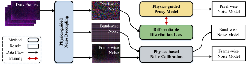
Figure 1: The overview of our physics-guided noise neural proxy (PNNP) framework. We have visualized the noise as sRGB images for viewing through a simple ISP pipeline.

3 Method

3.1 Strategy and Framework

To facilitate a clear understanding of our strategy and framework, we will begin with a brief overview of the general sensor imaging model.

During the sensor imaging process, the incident scene irradiance $I$ undergoes several transformations, including conversion to charges and subsequently voltages, amplification by amplifiers, and quantization into the digital signal $D$ by an analog-to-digital converter (ADC) [24]. For a raw image captured by a sensor, the imaging model can be expressed as

$$D=K(I+N_{p})+N_{indep},$$ (1)

where $K$ represents the overall system gain, $N_{p}$ is the signal-dependent photon shot noise, and $N_{indep}$ is signal-independent noise. The general noise model can be extracted as

$$N=KN_{p}+N_{indep}.$$ (2)

In the general noise model, the shot noise model based on the photoelectric effect is relatively reliable due to well-defined physical processes, which can be modeled as

$$(I+N_{p})\sim{\mathcal{P}(I)},$$ (3)

where $\mathcal{P}(\cdot)$ denotes the Poisson distribution. In contrast, the origin of signal-independent noise is highly complex, and there is no consensus on its noise model in the imaging community [47, 26, 24, 27, 22, 48]. In low-light conditions, the contribution of signal-independent noise is much higher compared to that in normal-light conditions, thus further emphasizing the need for accurate noise modeling.

To achieve accurate noise modeling, some advanced noise modeling methods [32, 33, 34] attempt to integrate physics-based methods into learning-based methods. However, as shown in Table I, they are bound by the dependency on high-quality paired real data, limiting their practicality. To release the noise modeling from the constraints of data dependency and further enhance the accuracy of noise modeling, we propose a novel strategy: learning the noise model from dark frames instead of paired real data. Motivated by this new strategy, we introduce a novel noise modeling framework, physics-guided noise neural proxy (PNNP), as shown in Fig. 1.

The first step of PNNP is physics-guided noise decoupling. Dark frames are the images captured under a lightless environment, which contains complete signal-independent noise. We decouple dark frames into three independent levels, which can be present as

$$N_{indep}=N_{frame}+N_{band}+N_{pixel},$$ (4)

where $N_{frame}$ represents the temporal stable frame-wise noise, $N_{band}$ represents the row- or col-related band-wise noise, and $N_{pixel}$ represents the independent and identically distributed (i.i.d.) pixel-wise noise.

We leverage the frame-wise noise and band-wise noise to calibrate their respective noise models using established physics-based noise calibration methods [13, 14, 49]. Notably, our primary focus lies in accurately modeling the pixel-wise noise, a challenging task for previous physics-based noise modeling methods. Therefore, we just employ a powerful neural network as the proxy model of pixel-wise noise. The decoupled pixel-wise noise exhibits the favorable characteristic of spatial independence, which serves as a valuable physical prior. To fully exploit the physical prior, we introduce the PPM to represent the pixel-wise noise and utilize the DDL to measure the distribution distance. Through precise and efficient training, we can obtain the pixel-wise noise model. Detailed implementation specifics of the PND, PPM, and DDL will be elaborated in subsequent sections of the paper.

In summary, the PNNP simplifies the complexity of noise modeling, combining the advantages of physics-based and learning-based approaches to enhance the accuracy of noise modeling.

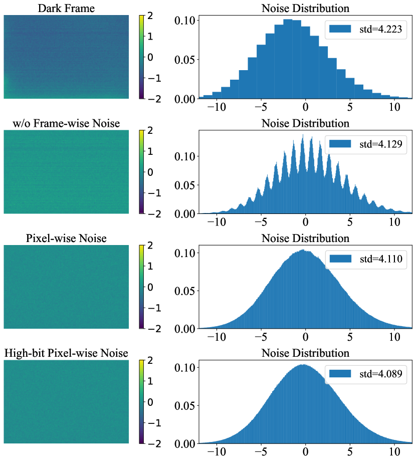
Figure 2: The analysis of PND process. The first and second columns plot the noise and its corresponding noise distribution, respectively. “std” refers to the standard deviation of the noise, which characterizes the intensity of the noise. The numerical range is adjusted for the best viewing.

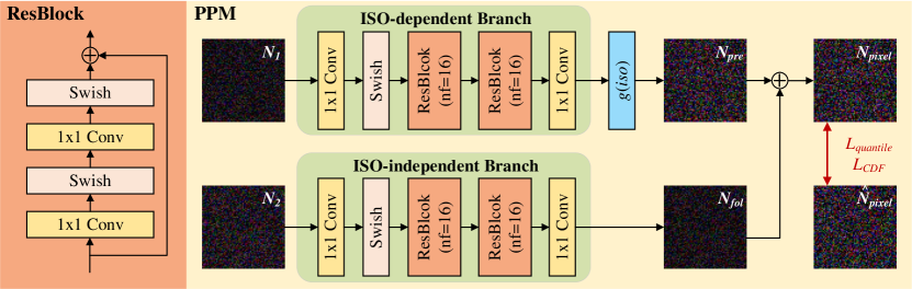
Figure 3: The overview of our PPM. “nf” represents the number of filters. All 1$\times$1 convolutions in PPM have 16 channels.

3.2 Physics-guided Noise Decoupling

In this section, we will introduce the principles and procedures of physics-guided noise decoupling in detail.

Previous research [49] highlights the advantages of noise decoupling in reducing data mapping complexity and improving denoising performance. We extend this notion to noise modeling, demonstrating that noise decoupling offers advantages beyond denoising. By employing different modeling approaches to address distinct levels of noise, we can effectively reduce the complexity of noise modeling. In line with the physical mechanisms and statistical characteristics of noise, we decouple dark frames into three independent noise types with significant mode differences: frame-wise noise, band-wise noise, and pixel-wise noise. The decoupling process of a dark frame is shown in Fig. 2. The notion of PND is that noise neural proxy should only focus on the unknown part of noise. Simplified real noise brings superiority to the learnability of data mapping.

Initially, the original dark frame, captured in a lightless environment, is represented as discrete signals with quantization intervals. In the decoupling process, we first employ frame-wise decoupling [17] to calibrate and eliminate the frame-wise noise $N_{frame}$. As a result, the dark frame devoid of frame-wise noise no longer exhibits significant spatial non-uniformity and retains various random noise components. Subsequently, we employ band-wise decoupling [14] to calibrate and eliminate the band-wise noise $N_{band}$, resulting in a dark frame without spatial correlation, where only i.i.d. pixel-wise noise remains. Due to the low-bit quantization of the original dark frame, the noise distribution of the pixel-wise noise exhibits periodic fluctuations caused by quantization-induced signal misalignment, as shown in Fig. 2. To mitigate the impact of quantization-induced signal misalignment on the noise neural proxy, we perform high-bit reconstruction [20] to eliminate the influence of quantization noise. The resulting high-bit pixel-wise noise $N_{pixel}$ serves as the ground truth for subsequent noise neural proxy modeling. The observed significant variations in noise distribution and noise intensity (standard deviation) in Fig. 2 indicate the effectiveness of our physics-guided noise decoupling.

Next, we will detail the principles and procedures of frame-wise decoupling, band-wise decoupling, and high-bit reconstruction, respectively.

Frame-wise noise, also known as dark shading [22], represents the temporal stable component of signal-independent noise and encompasses both spatial invariant Black Level Error (BLE) [52, 14] and spatial variant Fixed Pattern Noise (FPN) [25, 24, 27, 53, 48]. Following previous works [17], we first compute the average of dark frames at the same ISO to estimate the ISO-specific frame-wise noise. Then, we utilize a linear dark shading model to fit the ISO-specific frame-wise noise at different ISO as the final frame-wise noise model

$$N_{frame}=N_{FPNk}\cdot iso+N_{FPNb}+BLE(iso),$$ (5)

where $N_{FPNk}\in\mathbb{R}^{H\times W}$ and $N_{FPNb}\in\mathbb{R}^{H\times W}$ are the coefficient maps of the FPN that needs to be regressed, $iso$ is the ISO value, $BLE(iso)$ is the BLE at a specific ISO value $iso$. We introduce small perturbations to each parameter during training in order to simulate calibration errors.

The band-wise noise can be primarily divided into row noise $N_{row}$ and column noise $N_{col}$, which are typically associated with the working frequency and readout mechanism of the sensor circuit

$$N_{band}=N_{row}+N_{col}.$$ (6)

Following previous works [13, 14], we model the band-wise noise as zero-mean Gaussian noise

$$N_{row}\sim\mathcal{N}(0,\sigma^{2}_{row}),N_{col}\sim\mathcal{N}(0,\sigma^{2}_{col}),$$ (7)

where $N_{row}\in\mathbb{R}^{H\times 1}$ and $N_{col}\in\mathbb{R}^{1\times W}$.

The band-wise noise can be easily estimated by computing the mean of each row or column in the dark frames. The goodness of fit can be evaluated using the coefficient of determination in the probability plot, denoted as R² [54]. In our experiments, the R² for fitting the band-wise noise with a Gaussian distribution exceeds 0.999, indicating a strong adherence of the band-wise noise to the assumption of a Gaussian distribution.

After the aforementioned physics-guided noise decoupling, the remaining noise corresponds to the pixel-wise noise, which can be considered as the aggregation of all i.i.d. noise within the sensor. As introduced at the beginning of this section, the pixel-wise noise obtained from the noise decoupling exhibits quantization-induced signal misalignment. Therefore, we employ the high-bit reconstruction technique proposed in SFRN [20] to reconstruct the pixel-wise noise. It is worth noting that SFRN does not perform noise decoupling to high-bit reconstruction, resulting in non-i.i.d. signals that affect the accuracy of high-bit reconstruction. The effectiveness of the high-bit reconstruction technique relies on our noise decoupling strategy, which is not considered in existing works.

In summary, the physics-guided noise decoupling strategy simplifies the complexity of the noise modeling, thereby reducing the complexity of noise modeling.

3.3 Physics-guided Proxy Model

As shown in Fig. 3, we propose the PPM to constrain the optimization process based on physical priors. Our overall network architecture adopts a lightweight dual-branch design. The input of PPM is the random noise $N_{1}$ and $N_{2}$ that follows a standard normal distribution. We divide the input into two parts, which are separately fed into the ISO-dependent branch and the ISO-independent branch. Two branches of the network share identical structures, which include 1$\times$1 convolutions, Swish activation functions [55], and ResBlocks composed of these operations. Following the physical imaging process of sensors, the output $N_{pre}$ from the ISO-dependent branch undergoes amplification using a gain layer $g(iso)$, while the output $N_{fol}$ from the ISO-independent branch remains unchanged regardless of ISO variations. The sum of the outputs from these dual branches is pixel-wise noise $N_{pixel}$, representing the noise transformation result of our proxy model. We use the quantile loss $L_{quantile}$ and CDF loss $L_{CDF}$ to supervise the model, where the high-bit pixel-wise noise $\hat{N}_{pixel}$ is the ground truth. The process can be summarized as

$$N_{pixel}={\rm PPM}(N_{1},N_{2},iso),$$ (8)

where $N_{1},N_{2},N_{pixel}\in\mathbb{R}^{H\times W}$.

We will provide a detailed explanation of the two physics-guided designs incorporated in our network.

Firstly, we introduce the design of the pixel-wise independent module. Considering the i.i.d. nature of pixel-wise noise, all module designs utilize spatially independent operations, employing 1$\times$1 convolutions instead of 3$\times$3 convolutions. Despite the theoretical advantage of 3$\times$3 convolutions in terms of optimization freedom, as 3$\times$3 convolutions encompass the search space of 1$\times$1 convolutions, 3$\times$3 convolutions can pose an optimization trap in practical scenarios. The presence of non-zero parameters in 3$\times$3 convolutions (except the central parameter) introduces spatial correlation, which contradicts the prior assumption of pixel-wise spatial independence. It is worth emphasizing that most of learning-based methods [29, 30, 31, 32], including flow-based methods [28, 33], introduce spatial correlations. Moreover, the distinctive feature of PND, decoupling noise into spatially independent pixel-wise noise, is a sufficient condition where the efficacy of 1$\times$1 convolutions shines. Therefore, the usage of 1$\times$1 convolutions in the proxy model is simple yet nontrivial. By adhering to the structural constraint of 1$\times$1 convolutions, the proxy model significantly reduces its optimization freedom while adhering to the prior assumption of spatial independence.

Next, we introduce the design of the ISO-aware dual branch. The noise pattern is significantly affected by analog amplifiers in sensor circuits. Inspired by the physical principle of noise amplification in analog amplifiers, we divide the network into ISO-dependent and ISO-independent branches. Typically, sensor gains exhibit linear growth with ISO. Therefore, we design an ISO-dependent gain layer $g(iso)$ based on the linear gain prior, which is equivalent to the analog gain $K$. In this paper, we define the gain layer $g(iso)$ as a learnable look-up table (LUT) and initialize it with parameters obtained from noise calibration. By leveraging the explicit modeling of the ISO-aware dual branch network, the proxy model effectively bridges the noise model across different ISO levels while maintaining interpretability.

In summary, the physics-guided proxy model restricts the degrees of freedom during optimization based on physical priors, thereby promoting the accuracy of noise modeling.

3.4 Differentiable Distribution Loss

The choice of loss function poses a major challenge in learning-based noise modeling, as it is difficult to accurately measure the distance between noise distributions based on a set of noise. Previous methods can only measure the distribution through indirect approaches to train neural networks. A common approach is to employ Generative Adversarial Networks (GANs) [56]. GANs employ neural networks to extract noise features and estimate the distance between these features, indirectly quantifying the distance between noise distributions. However, GANs are known to be prone to instability and overfitting, often requiring careful initialization for effective convergence in noise modeling. Another common approach is to employ normalizing flow [50]. The invertible neural network of the flow-based model is bijective. By learning the transformation process from unknown real noise to known Gaussian noise, the model can simultaneously learn the reverse process, which is equivalent to noise modeling. However, the strict reversibility also limits the performance of flow-based models, leading to underfitting in noise models.

Our novel noise decoupling strategy introduces pixel-wise noise without spatial dependency, thereby presenting a fresh opportunity to design loss functions for noise modeling. We observe that the distribution function of i.i.d. pixel-wise noise can serve as a representation of the noise model itself. Motivated by this insight, we propose the DDL that leverages cumulative distribution functions (CDFs) for precise and interpretable measurements of the noise distribution. Instead of forcing complex data to fit measurement methods, we simplify the data to align with reliable measurement techniques.

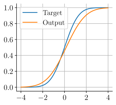
(a) Distribution Functions

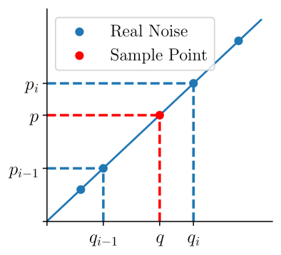
(b) Detailed View of CDF

Figure 4: The principle of DDL. (a) Cumulative distribution function plot, used to observe and measure the distribution distance between the target and the output. (b) Detailed view of CDF, used to illustrate the linear interpolation operation during the query process.

DDL incorporates two novel distribution losses: quantile loss $L_{quantile}$ and CDF loss $L_{CDF}$. Quantiles are values that divide a probability distribution into equal parts, while the CDF characterizes the probability of a random variable taking on a value less than or equal to a given value [54]. In Fig. 4(a), quantiles and CDF values form the horizontal and vertical axes of the cumulative distribution function plot, respectively. The CDF plot inspires us to measure the distance between distribution points using differences in their corresponding quantiles and CDF values, which forms the basis for $L_{quantile}$ and $L_{CDF}$.

Notably, to train neural networks with distribution loss functions, the entire loss computation procedure must be fully differentiable, despite the discrete nature of noisy samples. We exploit the property that sorting and normalization operations inherently preserve gradients, allowing us to derive a differentiable approximation of the CDF for these discrete data points. Consequently, this ensures the differentiability of both CDF querying and the overall loss computation pipeline.

For instance, when computing the CDF, given a set of $n$ noisy samples, the CDF of the $i$-th smallest value, $p_{i}$, is expressed as $F(i)=i/n$. To query the CDF, binary search locates the smallest index $i$ such that $q_{i}$ exceeds a given value $q$. As shown in Fig. 4(b), linear interpolation is then used to calculate the query result $p$ between adjacent samples $q_{i-1}$ and $q_{i}$:

$$p=F(q)=(i-\frac{q_{i}-q}{q_{i}-q_{i-1}})/n,$$ (9)

where negative infinity is appended to the dataset and adjustments are made to support arbitrary queries.

The above procedures involve solely differentiable operations, ensuring the differentiability of the distribution loss function. A similar but omitted approach is applied to derive the quantile loss.

Subsequently, we formally define our quantile loss $L_{quantile}$ and CDF loss $L_{CDF}$. For arbitrary pixel-wise noise $N_{pixel}$, its CDF is denoted as $F$, and its quantile function is denoted as $F^{-1}$. Given pixel-wise noise $N_{pixel}$, high-bit pixel-wise noise $\hat{N}_{pixel}$, and a set of query value sampling points $Q=\{q_{k}|k=1,2,...,N\}$, the CDF loss is defined as

$$L_{CDF}=\sum_{k=1}^{N}|F_{out}(q_{k})-F_{real}(q_{k})|,$$ (10)

where $F_{out}$ and $F_{real}$ represent the CDFs of pixel-wise noise $N_{pixel}$, high-bit pixel-wise noise $\hat{N}_{pixel}$, respectively.

Similarly, the quantile loss $L_{quantile}$ is defined as

$$L_{quantile}=\sum_{k=1}^{N}|F_{out}^{-1}(p_{k})-F_{real}^{-1}(p_{k})|,$$ (11)

where $F_{out}^{-1}$ and $F_{real}^{-1}$ represent the quantile functions of pixel-wise noise $N_{pixel}$, high-bit pixel-wise noise $\hat{N}_{pixel}$, respectively.

Each query operation typically provides supervision for only two samples around the query value. Therefore, the sampling strategy for query values plays a crucial role in the efficiency of the loss function. We design a random sampling strategy that introduces slight perturbations to fixed samples, enhancing the robustness of supervision. Initially, we use uniform sampling on the standard normal distribution as a baseline, covering the entire noise distribution in a uniform manner. Gaussian perturbations are then added around the baseline to increase the diversity of supervised points. We clip the query values to avoid numerical overflow.

In summary, the distribution loss function provides explicit and reliable supervision for the noise model, thereby promoting the precision of noise modeling.

TABLE II: Quantitative results (PSNR/SSIM) of different methods on the ELD dataset and SID dataset. The red color indicates the best results and the blue color indicates the second-best results.

	ELD Dataset [14]			SID Dataset [12]
Method	$\times$100	$\times$200	Average	$\times$100	$\times$250	$\times$300	Average
Paired Data	44.47 / 0.9676	41.97 / 0.9282	43.22 / 0.9479	42.06 / 0.9548	39.60 / 0.9380	36.85 / 0.9227	39.32 / 0.9374
P-G [23]	42.05 / 0.8721	38.18 / 0.7827	40.12 / 0.8274	39.44 / 0.8995	34.32 / 0.7681	30.66 / 0.6569	34.52 / 0.7666
ELD [14]	45.45 / 0.9754	43.43 / 0.9544	44.44 / 0.9649	41.95 / 0.9530	39.44 / 0.9307	36.36 / 0.9114	39.05 / 0.9303
SFRN [20]	46.38 / 0.9793	44.38 / 0.9651	45.38 / 0.9722	42.81 / 0.9568	40.18 / 0.9343	37.09 / 0.9175	39.82 / 0.9349
NoiseFlow [28]	43.21 / 0.9210	40.60 / 0.8638	41.90 / 0.8924	41.08 / 0.9394	37.45 / 0.8864	33.53 / 0.8132	37.09 / 0.8750
Starlight [32]	43.80 / 0.9358	40.86 / 0.8837	42.33 / 0.9098	40.47 / 0.9261	36.26 / 0.8575	33.00 / 0.7802	36.33 / 0.8494
LLD [33]	45.78 / 0.9789	44.08 / 0.9635	44.93 / 0.9712	42.29 / 0.9562	40.11 / 0.9373	36.89 / 0.9152	39.56 / 0.9348
LRD [34]	46.16 / 0.9829	43.91 / 0.9677	45.04 / 0.9753	43.16 / 0.9581	40.69 / 0.9406	37.48 / 0.9190	40.24 / 0.9378
PNNP (Ours)	47.31 / 0.9877	45.47 / 0.9791	46.39 / 0.9834	43.63 / 0.9614	41.49 / 0.9498	38.01 / 0.9353	40.83 / 0.9479

4 Experiment

4.1 Experimental Setting

4.1.1 Implementation details

Noise Modeling. The dark frames for noise modeling on the SID dataset [12] and ELD dataset [13, 14] are captured using a SonyA7S2 camera, which shares the same sensor as the public datasets but not the same camera. We prepare 5 dark frames per ISO for our PNNP. After physics-guided noise decoupling, we randomly crop 1024$\times$1024 patches at each step to train the PPM. We train the PPM with 1000 steps per ISO using Adam [57]. We sample 10⁶ query values per step according to the random sampling strategy of DDL. The learning rate follows a variation pattern similar to SGDR [58]. The base learning rate is set to 1$\times$10^-2 and the minimum learning rate is set to 1$\times$10^-5. The training setting on the LRID dataset [17] shares the same procedure.

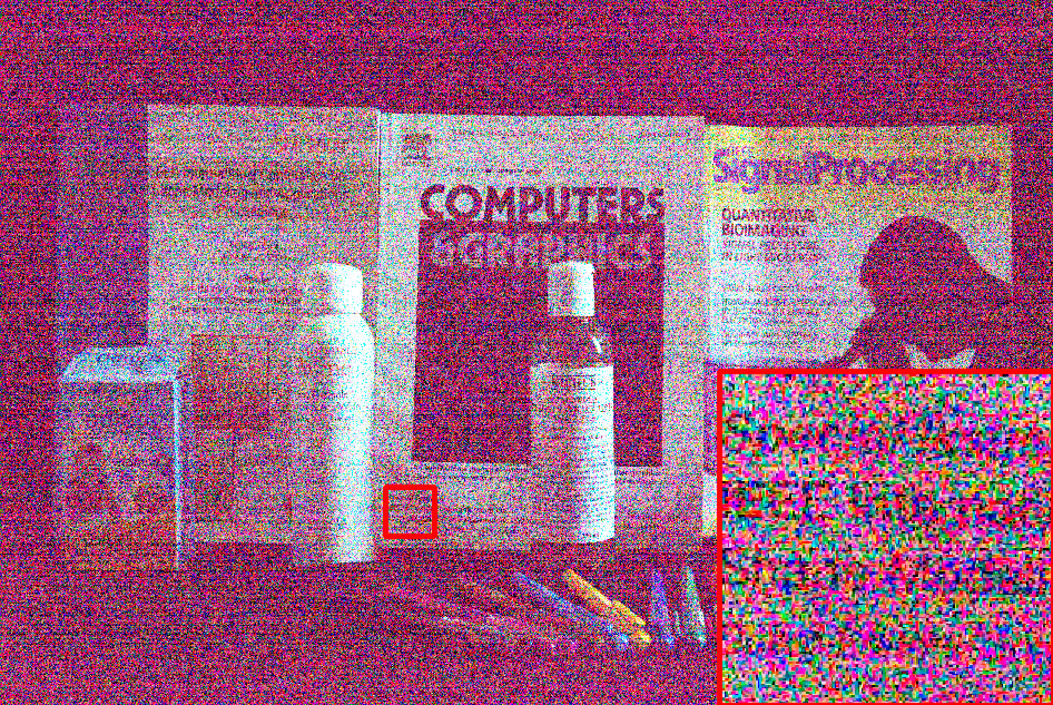
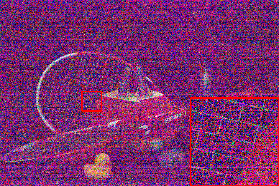
Noisy Image 21.48/0.1347 Noisy Image 22.32/0.0836

Reference Paired Data P-G[23] ELD[14] SFRN[20] PSNR/SSIM 36.76/0.9043 32.68/0.7412 37.63/0.9342 38.61/0.9467 NoiseFlow[28] Starlight[32] LLD[33] LRD[34] PNNP (Ours) 34.48/0.8126 34.56/0.8414 38.36/0.9460 38.40/0.9512 39.56/0.9650 Reference Paired Data P-G[23] ELD[14] SFRN[20] PSNR/SSIM 40.96/0.8788 37.41/0.7361 39.10/0.8164 43.86/0.9504 NoiseFlow[28] Starlight[32] LLD[33] LRD[34] PNNP (Ours) 43.07/0.9494 35.37/0.6497 43.12/0.9366 43.89/0.9454 45.80/0.9773

Figure 5: Raw image denoising results on images from the ELD dataset. The red color indicates the best results and the blue color indicates the second-best results. (Best viewed with zoom-in)

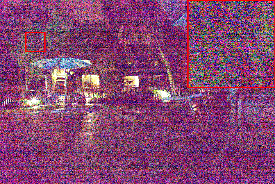
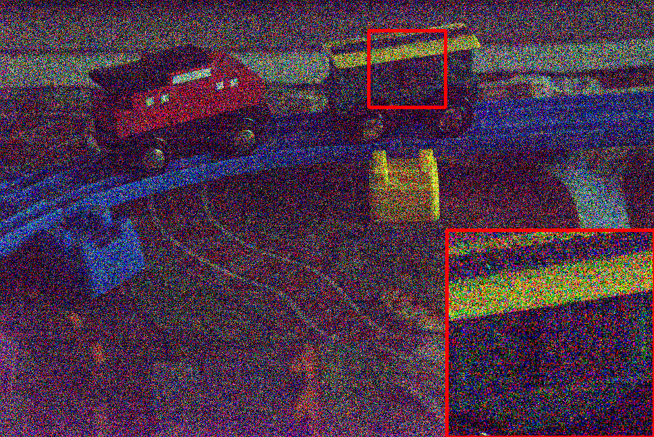
Noisy Image 18.33/0.088 Noisy Image 19.11/0.1075

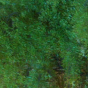
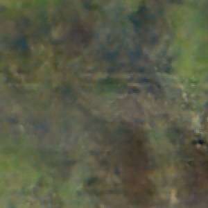
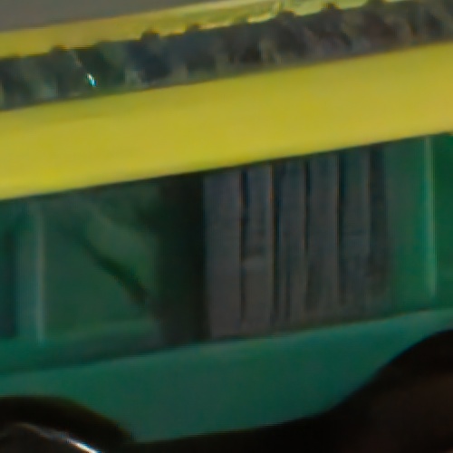
Reference Paired Data P-G[23] ELD[14] SFRN[20] PSNR/SSIM 32.16/0.8859 27.27/0.7293 32.21/0.8769 32.54/0.8834 NoiseFlow[28] Starlight[32] LLD[33] LRD[34] PNNP (Ours) 29.19/0.7943 28.67/0.8014 31.93/0.8754 32.46/0.8777 33.22/0.8970 Reference Paired Data P-G[23] ELD[14] SFRN[20] PSNR/SSIM 39.10/0.9447 29.78/0.6097 38.39/0.9424 39.52/0.9465 NoiseFlow[28] Starlight[32] LLD[33] LRD[34] PNNP (Ours) 34.06/0.8417 33.38/0.8228 39.45/0.9445 39.22/0.9450 40.51/0.9533

Figure 6: Raw image denoising results on images from the SID dataset. The red color indicates the best results and the blue color indicates the second-best results. (Best viewed with zoom-in)

Inspired by previous works [52, 13, 14], we record the errors associated with each type of noise (including linear dark shading) under the Gaussian error assumption during calibration. When synthesizing noise, we perturb the noise parameters based on these recorded errors, thereby endowing the denoising model with enhanced robustness.

Low-light Raw Image Denoising. We employ the same UNet architecture [59] as ELD for denoising. For the SID dataset and ELD dataset, we utilize raw images from the SID Sony training set to synthesize training data. The quantitative results are reported on the ELD Sony dataset and the whole SID Sony dataset, including validation and testing sets. For the LRID dataset, we synthesize training data based on the clean images in the training set. The quantitative results are reported on the official testing set. We adopt the dark shading correction strategy [17], thus we correct the frame-wise noise before inference. For training, we pack the raw images into four channels and crop each image into non-overlapping 512$\times$512 patches. These patches are then randomly rotated and flipped as a batch. We visualize the raw images as sRGB images for viewing through RawPy (a Python wrapper for LibRaw) based on the metadata of reference images. All of the quantitative results are computed on the raw images.

We train denoising models using Adam and $L_{1}$ loss. Each epoch consists of data pairs from various scenarios and exposure ratios. The learning rate will vary with iterations similar to SGDR. The entire training process comprises 1000 epochs, during which a single noisy image under each exposure ratio is traversed in each epoch. The training process includes two distinct stages: a coarse-tuning stage running for 600 epochs, initialized with a base learning rate of 2$\times$10^-4, and a subsequent fine-tuning stage extending over 400 epochs with a reduced base learning rate of 1$\times$10^-4. Both stages share the minimum learning rate of 1$\times$10^-5. The optimizer restarts every 200 epochs, accompanied by a halving of the learning rate upon each restart.

Compared Methods. In order to demonstrate the reliability of our PNNP, we compare our noise model with the following methods:

• The denoising model trained with paired real data (i.e., Paired Data), serves as a baseline for evaluating the performance of noise modeling applied to denoising.

• Physics-based noise modeling methods including P-G (Poisson-Gaussian) [23], ELD [14] and SFRN [20].

• Learning-based noise modeling methods including NoiseFlow [28], starlight [32], LLD [33] and LRD [34].

The results of P-G, ELD, SFRN, and Paired Data are implemented from the code and weights released by the open-source project [17]. The results of starlight and LLD are provided by the authors of LLD [33] Due to the lack of details, Learning-based noise modeling methods often pose a challenge to reproduce results meeting the claimed performance. Consequently, we just update the metrics of NoiseFlow based on our reproduced results. The results of starlight and LLD are sourced from the original authors of LLD, while the results of LRD are generated based on the official weights. On the LRID dataset, PNNP only compares with NoiseFlow among learning-based noise modeling methods.

It is important to emphasize that precisely measuring noise distribution discrepancies in real-world low-light image denoising datasets is impractical. On the one hand, classic distribution metrics, such as Kullback-Leibler Divergence (KLD) [54], are limited to characterize complex noise distributions under low-light conditions, as they are tailored for pixel-wise i.i.d. noise modeling [33]. On the other hand, inevitable data defects in the dataset, such as misalignments and residual noise, render the differences between clean data and noisy data inadequate for precisely representing the real noise distribution [17]. In response to these measurement complexities, we pivot towards adopting the performance of denoising networks trained on synthetic data generated by different noise modeling methods as the sole criterion for evaluation.

4.2 Denoising Results

4.2.1 ELD dataset and SID dataset

Table II summarizes the denoising performances over different exposure ratios based on different noise models. Fig. 5 and Fig. 6 shows the comparisons on ELD dataset and SID dataset, respectively.

The model trained with synthetic data based on physics-based noise models exhibits limited effectiveness in removing real-world noise. In low-light scenarios, the synthetic data generated by the P-G [23] lacks authenticity due to significant deviations from the real-world sensor noise model. As a result, denoising results exhibit noticeable color bias and stripe artifacts. While the ELD [14] enhances the modeling of signal-independent noise upon the P-G, it still falls short compared to the real-world sensor noise model. The absence of fixed-pattern noise modeling in the ELD leads to prominent pattern noise in denoising results and a failure to restore fine textures. In the case of the SFRN [20], which synthesizes data by sampling real signal-independent noise, the complexity of real noise poses challenges for the network to learn accurate data mappings. Therefore, persistent fixed-pattern noise remains in denoising results, indicating the potential for further improvement in restoring fine textures.

Learning-based noise modeling methods face challenges in ensuring the accuracy of the learned noise model. NoiseFlow [28] is limited by the representation ability of flow-based modules, which hinders NoiseFlow to precisely approximate complex noise distributions, resulting in significant blur. Starlight [32] seems to have not converged well due to the instability of GAN, resulting in obvious stripes and color bias. LLD [33] reduces the difficulty of noise approximation through noise decoupling. However, the flow-based backbone bound the representation ability of LLD, resulting in slight artifacts and color bias. Based on the Fourier Transformers, LRD [34] stands out as the state-of-the-art GAN-based method. Nonetheless, approximating complex noise distributions with neural networks remains a challenge, as evidenced by obvious stripes artifacts and blur.

In contrast, our method achieves the most exact color and clearest textures in the majority of scenarios in public datasets. Benefiting from accurate and precise noise modeling, the corresponding denoising results are free from obvious residual noise, encompassing complex fixed-pattern noise.

TABLE III: Quantitative results (PSNR/SSIM) of different methods on the LRID dataset. The red color indicates the best results and the blue color indicates the second-best results.

		NoiseFlow [28]	P-G [23]	ELD [14]	SFRN [20]	Paired Data	PNNP (Ours)
Dataset	Ratio	PSNR / SSIM	PSNR / SSIM	PSNR / SSIM	PSNR / SSIM	PSNR / SSIM	PSNR / SSIM
LRID-Indoor	$\times$64	48.16 / 0.9901	46.14 / 0.9872	48.19 / 0.9898	47.94 / 0.9899	48.77 / 0.9906	48.50 / 0.9908
	$\times$128	46.19 / 0.9828	44.98 / 0.9809	46.55 / 0.9836	46.52 / 0.9854	47.00 / 0.9860	46.94 / 0.9863
	$\times$256	43.91 / 0.9698	43.31 / 0.9682	44.39 / 0.9730	44.74 / 0.9789	44.74 / 0.9786	45.06 / 0.9797
	$\times$512	41.09 / 0.9442	40.80 / 0.9429	41.56 / 0.9452	42.46 / 0.9652	42.40 / 0.9647	42.64 / 0.9662
	$\times$1024	37.76 / 0.8906	37.74 / 0.8905	37.50 / 0.8915	40.10 / 0.9453	40.07 / 0.9437	40.30 / 0.9460
	Average	43.42 / 0.9555	42.59 / 0.9539	43.64 / 0.9566	44.35 / 0.9729	44.60 / 0.9727	44.69 / 0.9738
LRID-Outdoor	$\times$64	45.34 / 0.9856	42.16 / 0.9796	45.00 / 0.9841	45.05 / 0.9850	45.84 / 0.9876	45.62 / 0.9873
	$\times$128	43.82 / 0.9757	41.48 / 0.9709	43.48 / 0.9734	43.67 / 0.9766	44.50 / 0.9821	44.27 / 0.9821
	$\times$256	41.92 / 0.9570	40.36 / 0.9525	41.31 / 0.9450	41.89 / 0.9591	42.66 / 0.9709	42.63 / 0.9724
	Average	43.69 / 0.9728	41.33 / 0.9677	43.26 / 0.9675	43.54 / 0.9736	44.33 / 0.9802	44.17 / 0.9806

Input	NoiseFlow [28]	P-G [23]	ELD [14]	SFRN [20]	Paired Data	PNNP (Ours)	Reference
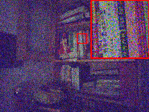
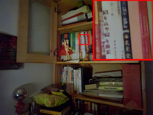
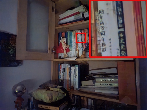
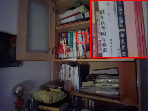
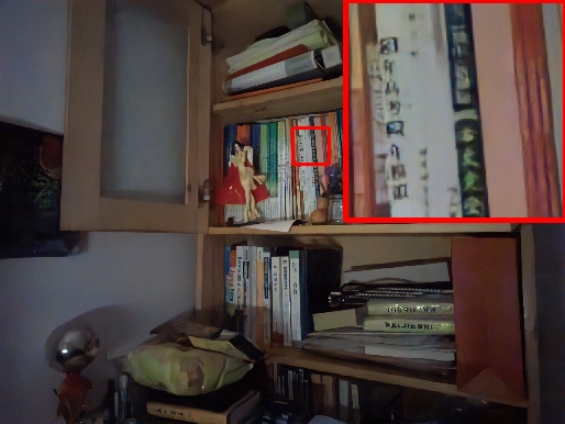
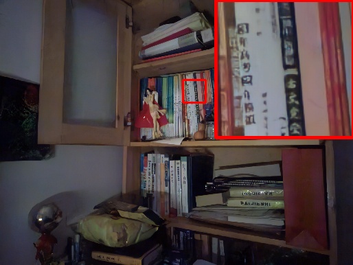
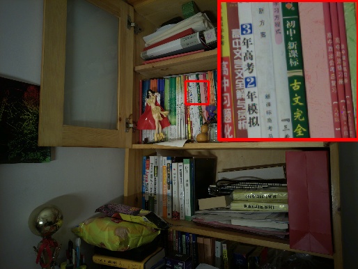
25.82 / 0.2597	45.14 / 0.9754	44.37 / 0.9721	45.27 / 0.9765	45.75 / 0.9810	45.41 / 0.9800	46.10 / 0.9825	PSNR / SSIM
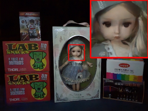
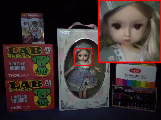
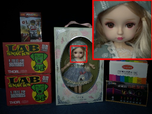
25.36 / 0.2236	41.94 / 0.9685	41.06 / 0.9653	41.92 / 0.9653	42.10 / 0.9735	42.40 / 0.9744	42.50 / 0.9751	PSNR / SSIM
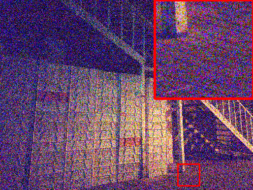
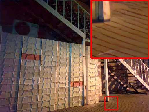
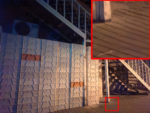
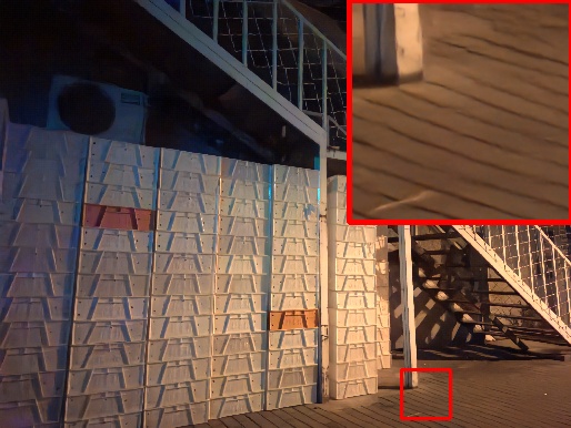
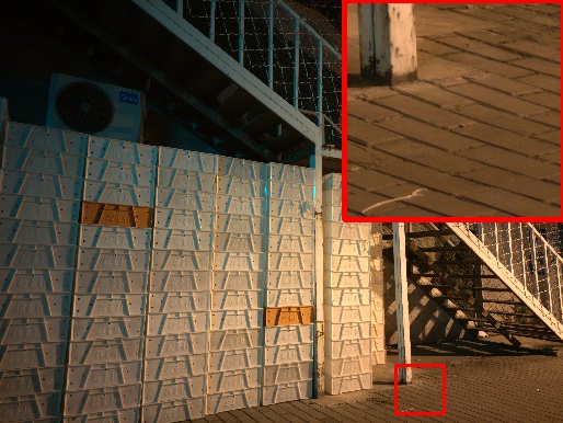
24.40 / 0.2593	40.70 / 0.9587	39.14 / 0.9506	40.49 / 0.9544	40.75 / 0.9625	40.95 / 0.9638	41.00 / 0.9650	PSNR / SSIM
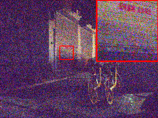
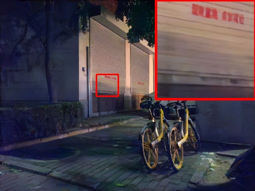
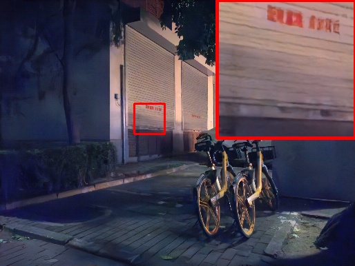
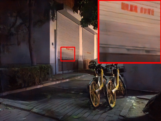
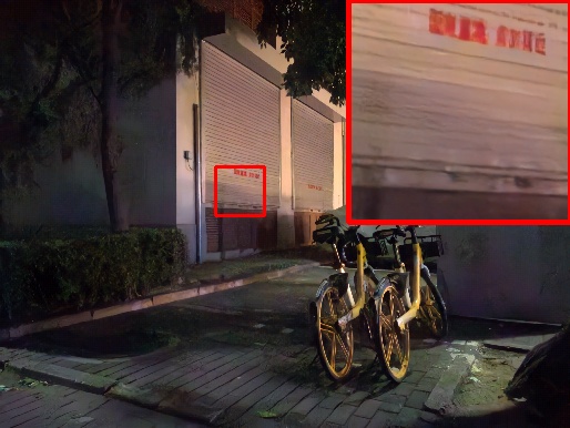
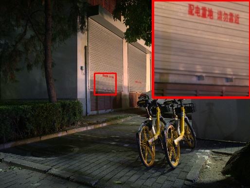
25.55 / 0.2505	43.03 / 0.9458	42.76 / 0.9468	41.19 / 0.9155	42.47 / 0.9367	44.81 / 0.9752	44.89 / 0.9760	PSNR / SSIM

Figure 7: Raw image denoising results on images from the LRID dataset. The red color indicates the best results and the blue color indicates the second-best results. (Best viewed with zoom-in)

4.2.2 LRID dataset

Table III summarizes the denoising performances over different exposure ratios based on different noise model. Fig. 7 shows the comparisons on some representative scenarios. The denoising performance rankings among noise modeling methods remain consistent with previous conclusions. Specifically, since the LRID dataset has fewer data defects compared to the SID dataset, the “Paired Data” serves as an exceptionally high baseline on the LRID dataset. Due to the high-quality data, learning-based methods depending on paired real data also exhibit improved performance. For instance, on the LRID dataset, NoiseFlow can be on par with or sometimes even outperform ELD. As mentioned in Table I, PNNP is independent of paired real data, therefore deriving minimal benefit from the improvement in data quality. Nonetheless, PNNP still demonstrates comparable denoising performance and further restore more details. The low data dependency and superior denoising performance demonstrate the practicality of our method.

4.3 Ablation Study

We conduct ablation studies from both the perspectives of noise modeling and image denoising to evaluate the effectiveness of our proposed contributions: PND, PPM, and DDL. The quantitative results of the ablation studies are shown in Table IV. We visualize a representative comparison of ablation studies at ISO-1600 in Fig. 8 and Fig. 9. All the ablation studies are performed on the SonyA7S2 camera.

TABLE IV: Ablation studies of proposed methods under different conditions. The metrics listed in the table are all averages over the dataset. The bold metrics indicate the best results.

Method	Condition	Noise Modeling		Image Denoising
		Pixel-wise Noise	Dark Frame Noise	ELD [14]	SID [12]
		KLD$\downarrow$ / R${}^{2}\uparrow$	KLD$\downarrow$ / R${}^{2}\uparrow$	PSNR$\uparrow$ / SSIM$\uparrow$	PSNR$\uparrow$ / SSIM$\uparrow$
	w/ Gaussian	0.00730 / 0.9682	0.02252 / 0.9603	40.12 / 0.8274	37.05 / 0.8255
	w/ ELD	0.01342 / 0.9837	0.02464 / 0.9685	44.44 / 0.9649	39.05 / 0.9303
	w/o Noise Decoupling	0.27335 / 0.9700	0.31421 / 0.9555	44.26 / 0.9591	38.45 / 0.9164
PND	PNNP (Ours)	0.00048 / 0.9995	0.01775 / 0.9789	46.39 / 0.9834	40.83 / 0.9479
	w/ Flow-based Module	0.00186 / 0.9932	0.01947 / 0.9724	46.00 / 0.9797	40.53 / 0.9444
	w/ 3$\times$3 Conv	0.00049 / 0.9994	0.01775 / 0.9789	44.69 / 0.9539	39.68 / 0.9213
	w/o Dual Branch	0.00500 / 0.9961	0.01784 / 0.9789	45.89 / 0.9727	40.55 / 0.9388
PPM	PNNP (Ours)	0.00048 / 0.9995	0.01775 / 0.9789	46.39 / 0.9834	40.83 / 0.9479
	w/o Quantile Loss	0.00203 / 0.9876	0.01986 / 0.9682	46.05 / 0.9806	40.67 / 0.9457
	w/o CDF Loss	0.00057 / 0.9994	0.01775 / 0.9789	46.16 / 0.9818	40.71 / 0.9466
DDL	PNNP (Ours)	0.00048 / 0.9995	0.01775 / 0.9789	46.39 / 0.9834	40.83 / 0.9479

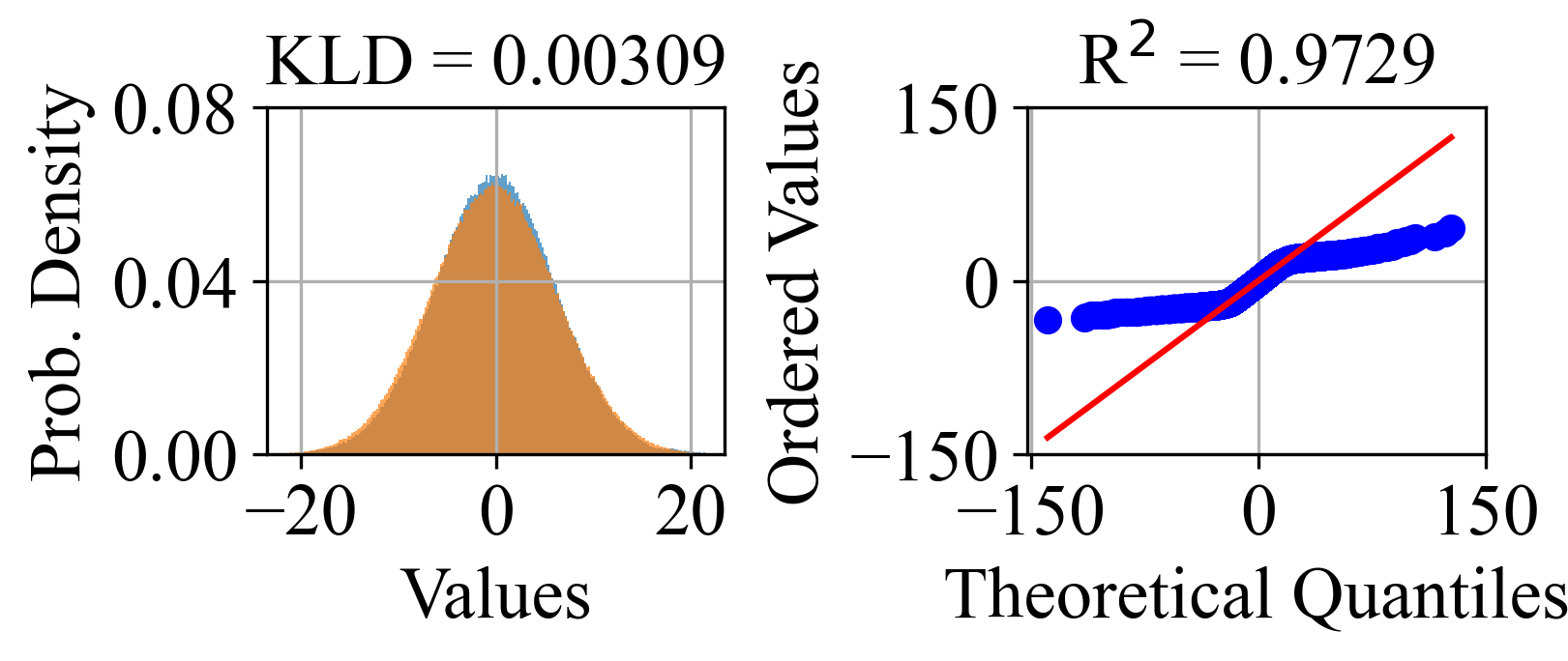
(a) w/ Gaussian

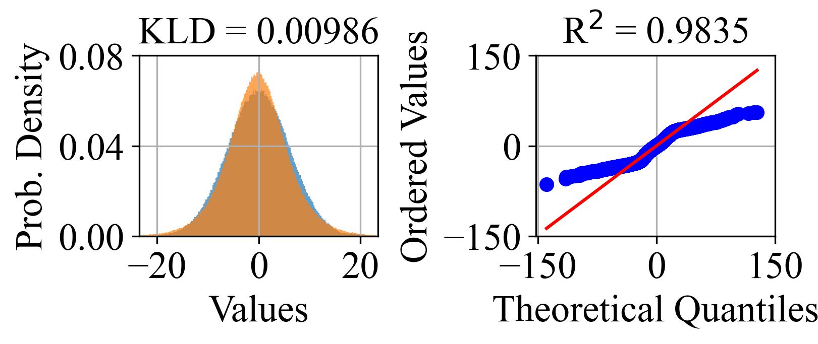
(b) w/ ELD

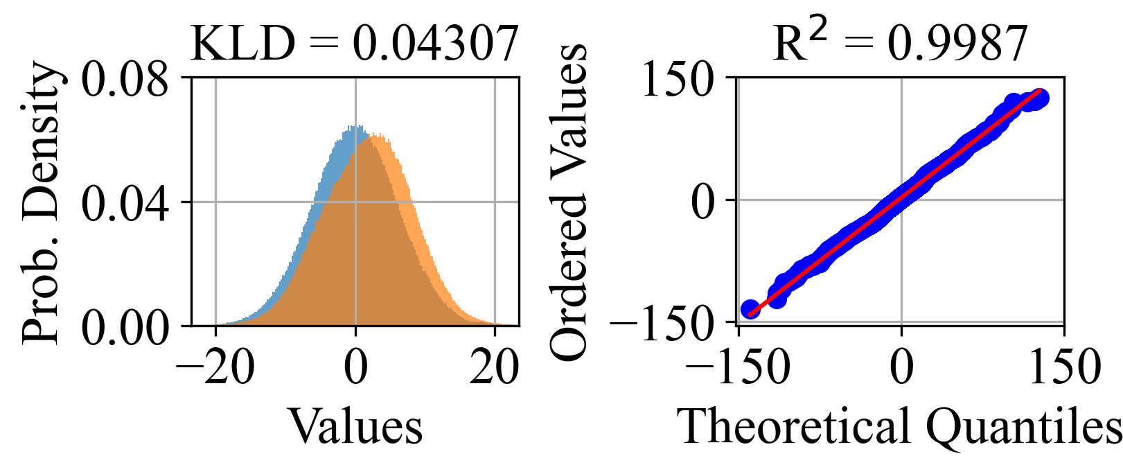
(c) w/o Noise Decoupling

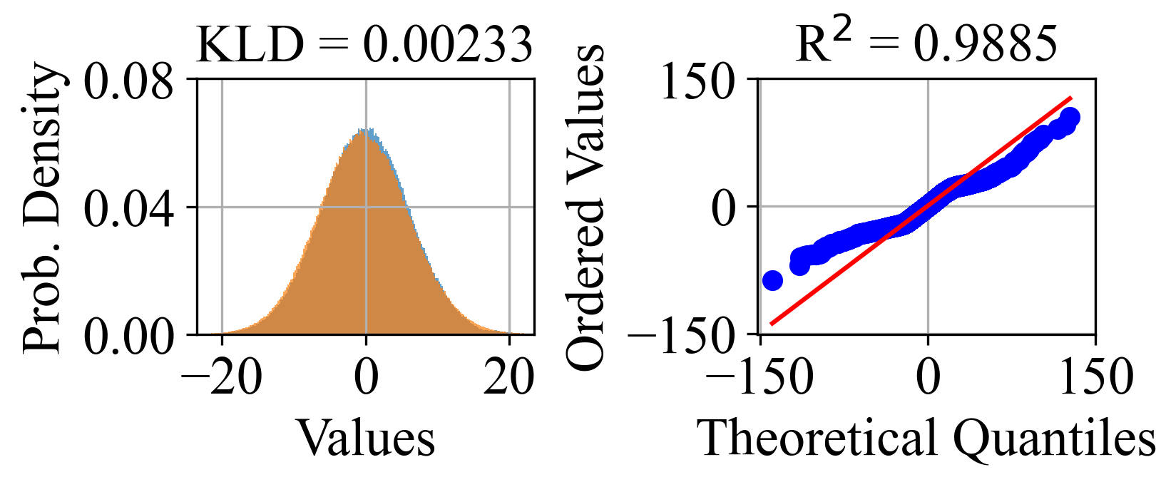
(d) w/ Flow-based Module

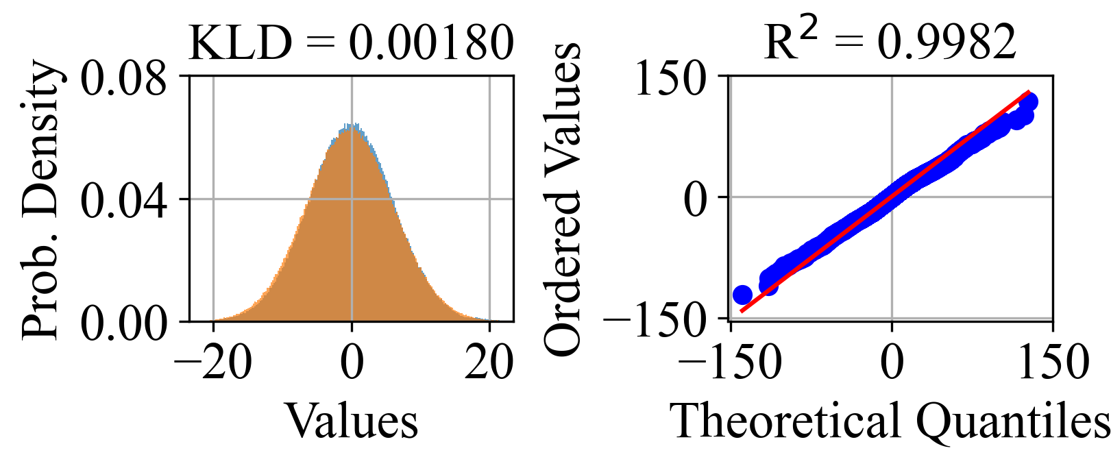
(e) w/ Conv3$\times$3

(f) w/o Dual Branch

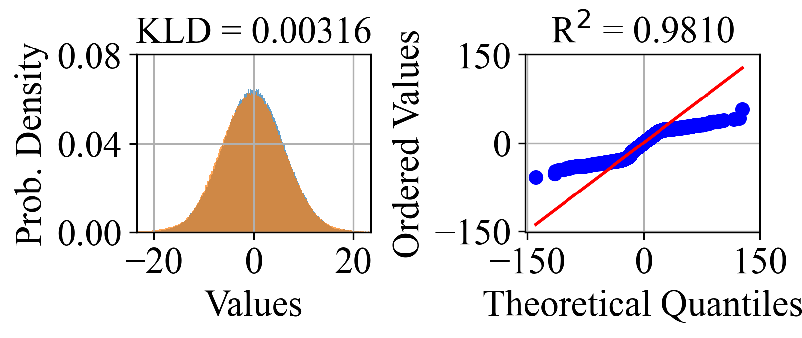
(g) w/o Quantile Loss Branch

(h) w/o CDF Loss Branch

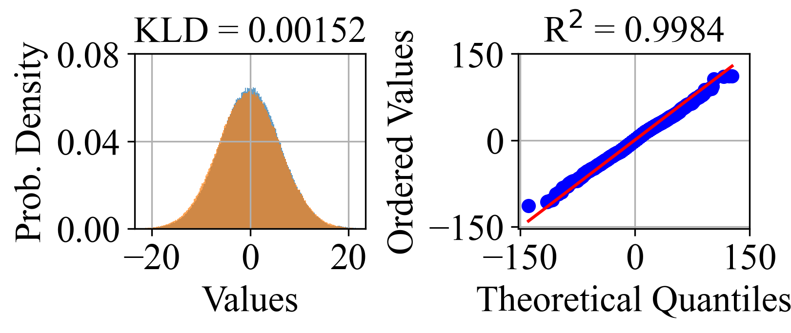
(i) PNNP (Ours)

Figure 8: A distribution comparison of ablation studies on pixel-wise noise at ISO-1600. Each subfigure consists of two parts: the left part shows a comparison of the probability density functions, while the right part shows the probability plot [54]. The blue histogram represents the distribution of real noise, while the orange histogram represents the distribution of synthetic noise. The blue points represent the quantiles of the real noise distribution, and the red line represents the quantiles of the synthetic noise distribution.

To evaluate the performance of noise modeling, we employ KLD and coefficient of determination (R²) as metrics on real noise [54]. Two types of real noise are used: pixel-wise noise and dark frame noise. Pixel-wise noise represents the high-bit pixel-wise noise decoupled by PND, which serves as the ground truth during training. Dark frame noise refers to the original dark frame without PND, which serves as the noise modeling target for our PNNP. The calculation process of KLD and R² is kept pace with the approaches described in NoiseFlow [28] and ELD [14], respectively.

To evaluate the performance of image denoising, we employ PSNR and SSIM as metrics on the public datasets. Since the metrics used for noise modeling cannot fully capture all the characteristics of the noise model, we consider the denoising performance corresponding to the noise model as the most important metric.

4.3.1 Ablation on PND

PND plays a vital role in bridging between physics-based noise modeling and learning-based noise modeling. To demonstrate its effectiveness, we select two classical physics-based noise modeling methods (Gaussian and ELD) as baselines and then explore the case of direct learning without noise decoupling. As shown in Table IV, compared to the classical physics-based noise modeling, PNNP retains substantial superiority in noise modeling. As shown in Fig. 8(a) and Fig. 8(b), both Gaussian and ELD exhibit low R², indicating their challenges in modeling long-tailed distributions. The comparison between Fig. 8(c) and Fig. 8(i) demonstrates the robust capability of our method in modeling long-tailed distributions. However, considering Table IV and Fig 9, PNNP without noise decoupling struggles to cover the complete noise distribution, leaving noticeable pattern noise residues, which indicates the indispensability of PND for the entire framework.

w/ Gaussian	w/ ELD	w/o Noise Decoupling	w/ Flow-based Module	w/ Conv3$\times$3
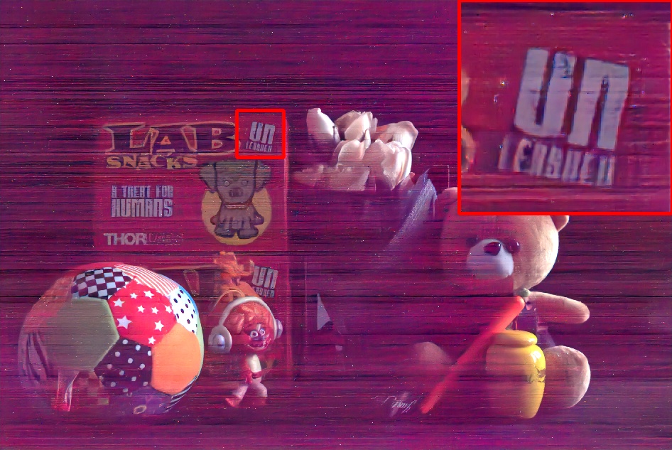
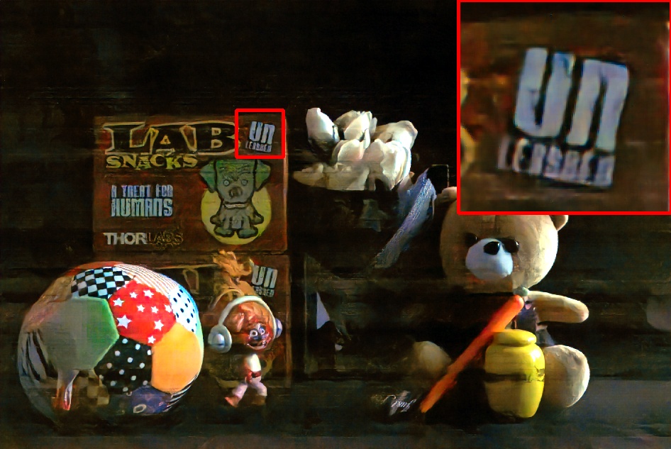
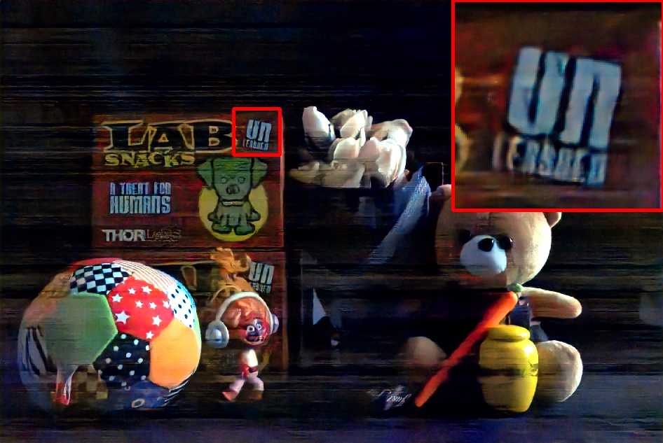
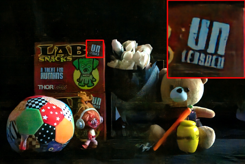
34.53 / 0.6103	42.75 / 0.9271	42.42 / 0.9174	44.17 / 0.9606	43.48 / 0.9469
w/o Dual Branch	w/o Quantile Loss	w/o CDF Loss	PNNP (Ours)	Reference
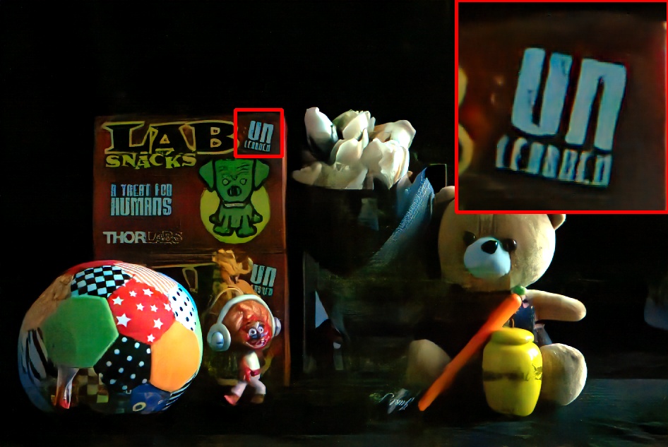
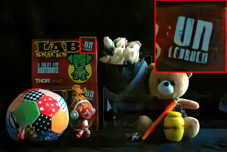
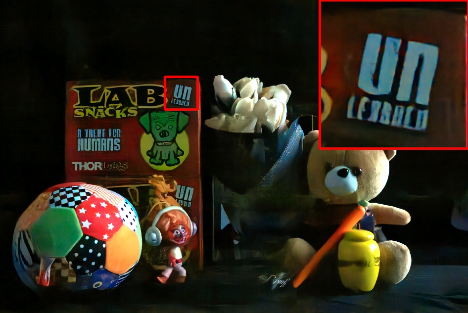
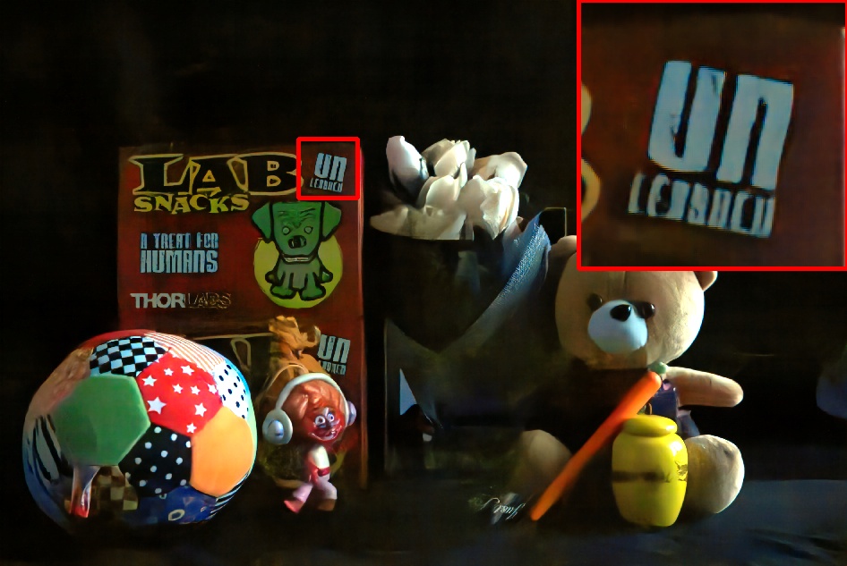
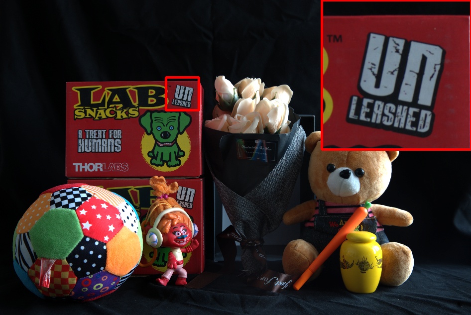
43.70 / 0.9332	44.20 / 0.9594	44.41 / 0.9636	44.70 / 0.9685	PSNR / SSIM

Figure 9: A representative visual comparison of ablation studies on the ELD dataset. The red color indicates the best results and the blue color indicates the second-best results. (Best viewed with zoom-in)

4.3.2 Ablation on PPM

To demonstrate the effectiveness of PPM, we first substitute the PPM modules with flow-based modules (marked as modified NoiseFlow) as a baseline, As shown in Fig. 8(d), the modified NoiseFlow performs well on KLD but falls short on R². Despite having more parameters than PNNP (2.7k vs. 2.2k), the modified NoiseFlow still struggles to approximate long-tailed distributions. Constrained by the limited representation ability of the flow model, DDL fails to bring significant improvements to the modified NoiseFlow.

Next, we will evaluate our physics-guided module designs proposed in PPM.

Our first design is using 1$\times$1 convolutions instead of 3$\times$3 convolutions to preserve the spatially independent prior of pixel-wise noise. In the ablation study, we replace all 1$\times$1 convolutions with 3$\times$3 convolutions. While the metrics for noise modeling may seem promising in Fig. 8(e), the corresponding denoising results exhibit noticeable residual pattern noise in Fig. 9. In the absence of explicitly considering spatially correlated noise components, the network spontaneously learns to exploit neighborhood information to optimize the noise model, inadvertently introducing spatial correlation. The unacceptable pattern noise highlights the significance of our pixel-wise independent module design.

Our second design is the network structure based on the sensor imaging mechanisms. In the ablation study, we change the ISO-aware dual-branch structure to a single branch. Without the physics-guided network structure design, the noise proxy model not only loses the physical interpretability but also exhibits a noticeable decrease in noise modeling, as shown in Fig. 8(f), which highlights the importance of our ISO-aware dual-branch design.

4.3.3 Ablation on DDL

DDL can be briefly divided into three components: quantile loss and CDF loss. We conducted an ablation study on each of these components, as shown in Table IV.

The quantile loss focuses on supervising the long-tail region of the noise distribution, which is consistent with the emphasis of R². Without quantile loss, the modeling ability on the long-tail distribution significantly decreases. It is reflected in the degradation of metrics in Fig 8(g) and the appearance of artifacts resembling defect pixels in denoising results, as shown in Fig. 9. The CDF loss focuses on supervising the central region of the noise distribution, which is the same as the emphasis of KLD. Without CDF loss, the modeling ability of PNNP slightly decreases, resulting in a slight decrease in KLD as shown in Fig 8(h). The complete DDL consistently provides reliable and stable supervision for PPM, contributing to the best performance in both noise modeling and corresponding image denoising results.

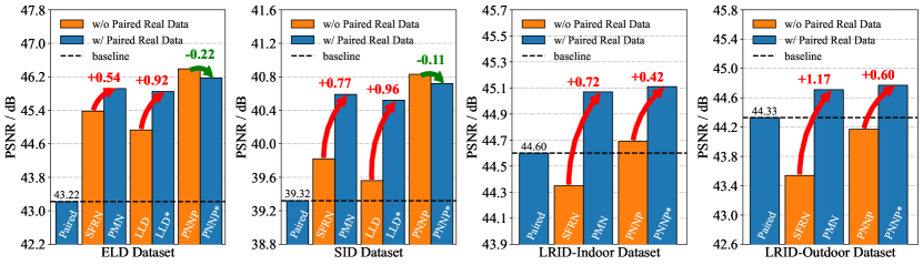
Figure 10: Comparison of denoising performance among noise modeling methods trained with and without paired real data. Arrows indicate changes in denoising performance after incorporating paired real data, with red arrows indicating positive gains and green arrows indicating negative gains.

Input	Paired Data	SFRN [20]	PMN [17]	LLD [33]	LLD* [33]	PNNP(Ours)	PNNP*(Ours)	Reference
22.58/0.0565	41.04/0.8590	47.19/0.9531	48.82/0.9811	46.82/0.9544	49.24/0.9808	49.83/0.9818	49.78/0.9822	PSNR/SSIM
33.64/0.7154	43.15/0.9767	45.05/0.9801	44.76/0.9819	44.56/0.9788	44.91/0.9818	45.90/0.9840	45.10/0.9808	PSNR/SSIM
23.56/0.2314	44.57/0.9862	44.32/0.9860	45.44/0.9894	- / -	- / -	44.98/0.9876	45.75/0.9901	PSNR/SSIM

Figure 11: Comparison of denoising performance among noise modeling methods trained with and without paired real data. We select some representative results from ELD dataset [14], SID dataset [12] and LRID datasets [17], respectively. (Best viewed with zoom-in)

5 Discussion

5.1 Data for Noise Modeling

One important premise often overlooked in noise modeling research is that real data is always essential in practical noise modeling. Learning-based approaches depend on real data to train noise models, while physics-based methods utilize real data for calibrating noise parameters. Although noise modeling methods are generally applicable, the model parameters exhibit sensor-specific characteristics. Hence, a robust and practical noise modeling approach should address the inherent challenges associated with real data quality.

The quality of real data directly influences the quality of the resulting noise model. The overlook for data is particularly severe in learning-based noise modeling methods. The existing strategy of learning-based noise modeling, which involves learning the clean-to-noise mapping from paired real data, has several problems from a data perspective. This strategy heavily depends on large-scale high-quality paired real data, which is often challenging to obtain. On one side, underdeveloped data acquisition protocol often results in signal misalignment within the paired real data. On the other side, the coupling of excessive noise models within the paired real data makes it challenging for neural networks to accurately approximate the real-world sensor noise model. In summary, data defects hinder the performance of the existing learning-based noise modeling strategy in practice.

Compared to learning-based noise modeling, physics-based noise modeling relies on real data collected by cameras specifically for calibration purposes, such as flat-field frames for calibrating signal-dependent noise and dark frames for calibrating signal-independent noise. The calibration process is independent of paired real data, eliminating signal misalignment. From the perspective of data dependency, the data required for physics-based noise modeling is easier to obtain and of higher quality compared to learning-based noise modeling.

Based on these insights, we propose the strategy of learning the noise model from dark frames instead of paired real data. The data-centric perspective [60] serves as the foundational principle guiding our analysis and problem-solving approach.

5.2 Integration of Paired Real Data and Noise Modeling

Recently, PMN [17] introduce a novel strategy that integrates paired real data and noise modeling, forming a kind of augmented hybrid data. Moreover, LLD [33] proposed a hybrid training strategy based on PMN, comprising two strategies: the dark shading correction strategy and the zero-mean noise strategy. The dark shading correction strategy relies on paired real data, while the zero-mean noise strategy relies on data synthesized based on noise modeling. By integrating the signal-independent noise model of LLD via the zero-mean noise strategy, LLD* achieves competitive performance in low-light denoising. The above hybrid-based methods not only involve noise modeling but also depend on the quality of paired real data. For the sake of controlling variables, we exclude them from comparisons in Section 4.2.

To facilitate a fair comparison with hybrid-based methods, we develop the noise augmentation method of PMN based on PNNP. PMN argues that only signal-dependent shot noise can be accurately modeled, thus proposing the shot noise augmentation (SNA) method to generate hybrid data. Fortunately, experiments in Section 4 have demonstrated the high precision of our PNNP in approximating signal-independent noise. Hence, inspired by SNA, we introduce a read noise augmentation method, supporting arbitrary interpolation between paired real data and synthetic data while maintaining the reliability of the noise model. We name the new hybrid-based method as PNNP*.

As shown in Table 10 and Fig. 11, we compare our method with existing hybrid-based methods and corresponding noise modeling methods. One of either PNNP or PNNP* consistently achieves state-of-the-art performance with exact color and clear details, demonstrating the superiority of our method.

A noteworthy difference emerges between PNNP and PNNP*, as detailed in Table 10, deserving an in-depth analysis. Intuitively, differences between paired real data are typically considered a reliable representation of real noise. Therefore, the introduction of paired real data in hybrid data is generally believed to promote the denoising performance. This assumption holds in most cases; however, the assumption fails between PNNP and PNNP* on the ELD dataset and SID dataset. This counterintuitive phenomenon aligns with our emphasis on data quality in Section 5.1. The denoising performance of hybrid-based methods depends not only on the accuracy of noise modeling but also on the quality of paired real data. The SID dataset exhibits noticeable data defects, including residual noise, spatial misalignment, and intensity discrepancies. These defects reduce the reliability of data mapping between paired real data, resulting in PNNP* trained on the SID dataset performing less effectively than PNNP. The LRID dataset overcomes most of the data defects, making the model trained only on paired real data competitive with PNNP. The complementarity of high-quality paired real data and a large amount of realistic synthetic data (generated by PNNP) leads to superior performance for PNNP* trained on the LRID dataset.

Finally, we note the efficient method proposed by LED [61], which requires only a small amount of paired real data to adapt a denoising method to new noise models. LED shares a similar motivation with hybrid-based methods; however, it lacks the process of noise modeling. Furthermore, LED also encounters challenges associated with the quality of paired real data, resulting in suboptimal denoising performance (LED is notably inferior to SFRN). Hence, in this paper, we refrain from comparing our approach with LED.

6 Conclusion

In this paper, we propose a novel strategy for noise modeling: learning the noise model from dark frames instead of paired real data. Based on the new strategy, we introduce a physics-guided noise neural proxy framework. Our framework leverages the physical priors of the sensor to decouple the complex noise, constrain the optimization process, and provide reliable supervision, thereby further improving the performance of noise modeling. Firstly, we propose a physics-guided noise decoupling strategy to handle different levels of noise in a flexible manner. Secondly, we propose a physics-guided proxy model incorporating physical priors to constrain the generated noise. Finally, we propose a differentiable distribution loss function to efficiently supervise the random noise variables. Benefiting from physics-guided designs, PNNP not only exhibits low data dependency but also facilitates easy training. These user-friendly features emphasize the practicality of PNNP. Experimental results on extensive low-light raw image denoising datasets demonstrate the superiority of our PNNP, highlighting its effectiveness and practicality in noise modeling.

Hansen Feng received the BS degree from the University of Science and Technology Beijing, China, in 2020. He is currently a Ph.D. student with the School of Computer Science and Technology, Beijing Institute of Technology. His research interests include computational photography and image processing. He received the Best Paper Runner-Up Award of ACM MM 2022.

Lizhi Wang (M’17) received the B.S. and Ph.D. degrees from Xidian University, Xi’an, China, in 2011 and 2016, respectively. He is currently an Associate Professor with the School of Computer Science and Technology, Beijing Institute of Technology. His research interests include computational photography and image processing. He received the Best Paper Award of IEEE VCIP 2016.

Yiqi Huang received the B.S. degree from the school of Information Science and Engineering, Lanzhou University, Lanzhou, China, in 2022. He is currently a M.D. student with the School of Computer Science and Technology, Beijing Institute of Technology. His research interests include computational photography and image processing.

Yuzhi Wang received the B.S. degree from the School of Telecommunication Engineering, Xidian University, Xi’an, China, in 2012. He received the Ph.D. degree with the Department of Electronic Engineering, Tsinghua University, Beijing, China, under the supervision of Prof. H. Yang. His research interests include wireless sensor networks, computational photography, machine learning, and deep neural networks

Lin Zhu (M’22) received the B.S. degree in computer science from the Northwestern Polytechnical University, China, in 2014, the M.S. degree in computer science from the North Automatic Control Technology Institute, China, in 2018, and the Ph.D. degree with the School of Electronics Engineering and Computer Science, Peking University, China, in 2022. He is currently an assistant professor with the School of Computer Science, Beijing Institute of Technology, China. His current research interests include image processing, computer vision, neuromorphic computing, and spiking neural network.

Hua Huang (SM’19) received the B.S. and Ph.D. degrees from Xi’an Jiaotong University, in 1996 and 2006, respectively. He is currently a professor in the School of Artificial Intelligence, Beijing Normal University. He is also an adjunct professor at Xi’an Jiaotong University and Beijing Institute of Technology. His main research interests include image and video processing, computational photography, and computer graphics. He received the Best Paper Award of ICML2020 / EURASIP2020 / PRCV2019 / ChinaMM2017.

References

- [1] K. Zhang, W. Zuo, Y. Chen, D. Meng, and L. Zhang, “Beyond a gaussian denoiser: Residual learning of deep cnn for image denoising,” IEEE Transactions on Image Processing (TIP), vol. 26, pp. 3142–3155, 2017.
- [2] K. Zhang, W. Zuo, and L. Zhang, “Ffdnet: Toward a fast and flexible solution for cnn-based image denoising,” IEEE Transactions on Image Processing (TIP), vol. 27, no. 9, pp. 4608–4622, 2018.
- [3] S. Guo, Z. Yan, K. Zhang, W. Zuo, and L. Zhang, “Toward convolutional blind denoising of real photographs,” in IEEE/CVF Conference on Computer Vision and Pattern Recognition (CVPR), 2019, pp. 1712–1722.
- [4] Z. Yue, H. Yong, Q. Zhao, D. Meng, and L. Zhang, “Variational denoising network: Toward blind noise modeling and removal,” Advances in Neural Information Processing Systems (NeurIPS), vol. 32, 2019.
- [5] S. W. Zamir, A. Arora, S. Khan, M. Hayat, F. S. Khan, M.-H. Yang, and L. Shao, “Multi-stage progressive image restoration,” in IEEE/CVF Conference on Computer Vision and Pattern Recognition (CVPR), 2021, pp. 14 821–14 831.
- [6] S. Cheng, Y. Wang, H. Huang, D. Liu, H. Fan, and S. Liu, “Nbnet: Noise basis learning for image denoising with subspace projection,” in IEEE/CVF Conference on Computer Vision and Pattern Recognition (CVPR), 2021, pp. 4896–4906.
- [7] L. Chen, X. Lu, J. Zhang, X. Chu, and C. Chen, “Hinet: Half instance normalization network for image restoration,” in IEEE/CVF Conference on Computer Vision and Pattern Recognition (CVPR), 2021, pp. 182–192.
- [8] J. Liang, J. Cao, G. Sun, K. Zhang, L. Van Gool, and R. Timofte, “Swinir: Image restoration using swin transformer,” in IEEE/CVF Conference on Computer Vision and Pattern Recognition (CVPR), 2021, pp. 1833–1844.
- [9] S. W. Zamir, A. Arora, S. Khan, M. Hayat, F. S. Khan, and M.-H. Yang, “Restormer: Efficient transformer for high-resolution image restoration,” in IEEE/CVF Conference on Computer Vision and Pattern Recognition (CVPR), 2022, pp. 5728–5739.
- [10] T. Plötz and S. Roth, “Benchmarking denoising algorithms with real photographs,” in IEEE/CVF Conference on Computer Vision and Pattern Recognition (CVPR), 2017, pp. 2750–2759.
- [11] A. Abdelhamed, S. Lin, and M. S. Brown, “A high-quality denoising dataset for smartphone cameras,” in IEEE/CVF Conference on Computer Vision and Pattern Recognition (CVPR), 2018, pp. 1692–1700.
- [12] C. Chen, Q. Chen, J. Xu, and V. Koltun, “Learning to see in the dark,” in IEEE/CVF Conference on Computer Vision and Pattern Recognition (CVPR), 2018, pp. 3291–3300.
- [13] K. Wei, Y. Fu, J. Yang, and H. Huang, “A physics-based noise formation model for extreme low-light raw denoising,” in IEEE/CVF Conference on Computer Vision and Pattern Recognition (CVPR), 2020, pp. 2755–2764.
- [14] K. Wei, Y. Fu, Y. Zheng, and J. Yang, “Physics-based noise modeling for extreme low-light photography,” IEEE Transactions on Pattern Analysis and Machine Intelligence (TPAMI), pp. 1–18, 2021.
- [15] B. Zhang, Y. Guo, R. Yang, Z. Zhang, J. Xie, J. Suo, and Q. Dai, “Darkvision: A benchmark for low-light image/video perception,” arXiv preprint arXiv:2301.06269, 2023.
- [16] H. Yue, C. Cao, L. Liao, and J. Yang, “Rvideformer: Efficient raw video denoising transformer with a larger benchmark dataset,” arXiv preprint arXiv:2305.00767, 2023.
- [17] H. Feng, L. Wang, Y. Wang, H. Fan, and H. Huang, “Learnability enhancement for low-light raw image denoising: A data perspective,” IEEE Transactions on Pattern Analysis and Machine Intelligence (TPAMI), pp. 1–18, 2023.
- [18] T. Brooks, B. Mildenhall, T. Xue, J. Chen, D. Sharlet, and J. T. Barron, “Unprocessing images for learned raw denoising,” in IEEE/CVF Conference on Computer Vision and Pattern Recognition (CVPR), 2019, pp. 11 036–11 045.
- [19] Y. Wang, H. Huang, Q. Xu, J. Liu, Y. Liu, and J. Wang, “Practical deep raw image denoising on mobile devices,” in European Conference on Computer Vision (ECCV), 2020, pp. 1–16.
- [20] Y. Zhang, H. Qin, X. Wang, and H. Li, “Rethinking noise synthesis and modeling in raw denoising,” in IEEE/CVF International Conference on Computer Vision (ICCV), 2021, pp. 4573–4581.
- [21] G. E. Healey and R. Kondepudy, “Radiometric ccd camera calibration and noise estimation,” IEEE Transactions on Pattern Analysis and Machine Intelligence (TPAMI), vol. 16, no. 3, pp. 267–276, 1994.
- [22] J. Nakamura, Image Sensors and Signal Processing for Digital Still Cameras. CRC press, 2017.
- [23] A. Foi, M. Trimeche, V. Katkovnik, and K. Egiazarian, “Practical poissonian-gaussian noise modeling and fitting for single-image raw-data,” IEEE Transactions on Image Processing (TIP), vol. 17, no. 10, pp. 1737–1754, 2008.
- [24] B. Jähne, “Emva 1288 standard for machine vision: Objective specification of vital camera data,” Optik & Photonik, vol. 5, no. 1, pp. 53–54, 2010.
- [25] G. C. Holst and T. S. Lomheim, CMOS/CCD Sensors and Camera Systems, Second Edition. SPIE, 2011.
- [26] R. Gow, D. Renshaw, K. Findlater, L. A. Grant, S. Mcleod, J. Hart, and R. Nicol, “A comprehensive tool for modeling cmos image-sensor-noise performance,” IEEE Transactions on Electron Devices (TED), vol. 54, pp. 1321–1329, 2007.
- [27] M. Konnik and J. Welsh, “High-level numerical simulations of noise in ccd and cmos photosensors: Review and tutorial,” arXiv preprint arXiv:1412.4031, pp. 1–21, 2014.
- [28] A. Abdelhamed, M. A. Brubaker, and M. S. Brown, “Noise flow: Noise modeling with conditional normalizing flows,” in IEEE/CVF International Conference on Computer Vision (ICCV), 2019, pp. 3165–3173.
- [29] Z. Yue, Q. Zhao, L. Zhang, and D. Meng, “Dual adversarial network: Toward real-world noise removal and noise generation,” in European Conference on Computer Vision (ECCV), 2020, pp. 41–58.
- [30] K.-C. Chang, R. Wang, H.-J. Lin, Y.-L. Liu, C.-P. Chen, Y.-L. Chang, and H.-T. Chen, “Learning camera-aware noise models,” in European Conference on Computer Vision (ECCV), 2020, pp. 343–358.
- [31] Y. Cai, X. Hu, H. Wang, Y. Zhang, H. Pfister, and D. Wei, “Learning to generate realistic noisy images via pixel-level noise-aware adversarial training,” in Advances in Neural Information Processing Systems (NeurIPS), vol. 34, 2021, pp. 3259–3270.
- [32] K. Monakhova, S. R. Richter, L. Waller, and V. Koltun, “Dancing under the stars: Video denoising in starlight,” in IEEE/CVF Conference on Computer Vision and Pattern Recognition (CVPR), 2022, pp. 16 241–16 251.
- [33] Y. Cao, M. Liu, S. Liu, X. Wang, L. Lei, and W. Zuo, “Physics-guided iso-dependent sensor noise modeling for extreme low-light photography,” in IEEE/CVF Conference on Computer Vision and Pattern Recognition (CVPR), 2023, pp. 5744–5753.
- [34] F. Zhang, B. Xu, Z. Li, X. Liu, Q. Lu, C. Gao, and N. Sang, “Towards general low-light raw noise synthesis and modeling,” in Proceedings of the IEEE/CVF International Conference on Computer Vision, 2023, pp. 10 820–10 830.
- [35] I. S. McLean, Electronic Imaging in Astronomy: Detectors and Instrumentation. Springer Science & Business Media, 2008.
- [36] M. S. Joens, C. Huynh, J. M. Kasuboski, D. Ferranti, Y. J. Sigal, F. Zeitvogel, M. Obst, C. J. Burkhardt, K. P. Curran, S. H. Chalasani et al., “Helium ion microscopy (him) for the imaging of biological samples at sub-nanometer resolution,” Scientific reports, vol. 3, no. 1, pp. 1–7, 2013.
- [37] S. W. Hasinoff, D. Sharlet, R. Geiss, A. Adams, J. T. Barron, F. Kainz, J. Chen, and M. Levoy, “Burst photography for high dynamic range and low-light imaging on mobile cameras,” ACM Transactions on Graphics (TOG), vol. 35, no. 6, pp. 1–12, 2016.
- [38] M. Aharon, M. Elad, and A. Bruckstein, “K-svd: An algorithm for designing overcomplete dictionaries for sparse representation,” IEEE Transactions on Signal Processing (TSP), vol. 54, no. 11, pp. 4311–4322, 2006.
- [39] M. Elad and M. Aharon, “Image denoising via sparse and redundant representations over learned dictionaries,” IEEE Transactions on Image Processing (TIP), vol. 15, no. 12, pp. 3736–3745, 2006.
- [40] S. Gu, L. Zhang, W. Zuo, and X. Feng, “Weighted nuclear norm minimization with application to image denoising,” in IEEE/CVF Conference on Computer Vision and Pattern Recognition (CVPR), 2014, pp. 2862–2869.
- [41] A. Buades, B. Coll, and J.-M. Morel, “A non-local algorithm for image denoising,” in IEEE/CVF Conference on Computer Vision and Pattern Recognition (CVPR), 2005, pp. 60–65.
- [42] K. Dabov, A. Foi, V. Katkovnik, and K. Egiazarian, “Image denoising by sparse 3-d transform-domain collaborative filtering,” IEEE Transactions on Image Processing (TIP), vol. 16, pp. 2080–2095, 2007.
- [43] J. Portilla, V. Strela, M. J. Wainwright, and E. P. Simoncelli, “Image denoising using scale mixtures of gaussians in the wavelet domain,” IEEE Transactions on Image Processing (TIP), vol. 12, no. 11, pp. 1338–1351, 2003.
- [44] L. I. Rudin, S. Osher, and E. Fatemi, “Nonlinear total variation based noise removal algorithms,” Physica D: nonlinear phenomena, vol. 60, no. 14, pp. 259–268, 1992.
- [45] C. Chen, Q. Chen, M. N. Do, and V. Koltun, “Seeing motion in the dark,” in IEEE/CVF International Conference on Computer Vision (ICCV), 2019, pp. 3185–3194.
- [46] C. Li, C. Guo, L.-H. Han, J. Jiang, M.-M. Cheng, J. Gu, and C. C. Loy, “Low-light image and video enhancement using deep learning: A survey,” IEEE Transactions on Pattern Analysis and Machine Intelligence (TPAMI), pp. 1–19, 2021.
- [47] H. Wach and E. R. Dowski Jr, “Noise modeling for design and simulation of computational imaging systems,” in Visual Information Processing, 2004, pp. 159–170.
- [48] L. Song and H. Huang, “Fixed pattern noise removal based on a semi-calibration method,” IEEE Transactions on Pattern Analysis and Machine Intelligence (TPAMI), pp. 1–14, 2023.
- [49] H. Feng, L. Wang, Y. Wang, and H. Huang, “Learnability enhancement for low-light raw denoising: Where paired real data meets noise modeling,” in Proceedings of the 30th ACM International Conference on Multimedia (ACMMM), 2022, pp. 1436–1444.
- [50] D. P. Kingma and P. Dhariwal, “Glow: Generative flow with invertible 1x1 convolutions,” in Advances in Neural Information Processing Systems (NeurIPS), S. Bengio, H. Wallach, H. Larochelle, K. Grauman, N. Cesa-Bianchi, and R. Garnett, Eds., vol. 31, 2018, pp. 1–10.
- [51] L. D. Tran, S. M. Nguyen, and M. Arai, “Gan-based noise model for denoising real images,” in Proceedings of the Asian Conference on Computer Vision (ACCV), 2020.
- [52] J. Wang, Y. Yu, S. Wu, C. Lei, and K. Xu, “Rethinking noise modeling in extreme low-light environments,” in IEEE International Conference on Multimedia and Expo (ICME), 2021, pp. 1–6.
- [53] M. Maggioni, E. Sánchez-Monge, and A. Foi, “Joint removal of random and fixed-pattern noise through spatiotemporal video filtering,” IEEE Transactions on Image Processing (TIP), vol. 23, no. 10, pp. 4282–4296, 2014.
- [54] E. L. Lehmann, J. P. Romano, and G. Casella, Testing statistical hypotheses. Springer, 1986, vol. 3.
- [55] P. Ramachandran, B. Zoph, and Q. V. Le, “Searching for activation functions,” in International Conference on Learning Representations (ICLR), 2018, pp. 1–13.
- [56] I. Goodfellow, J. Pouget-Abadie, M. Mirza, B. Xu, D. Warde-Farley, S. Ozair, and Y. Bengio, “Generative adversarial networks, 1–9,” in Advances in Neural Information Processing Systems (NeurIPS), vol. 27, 2014, pp. 1–9.
- [57] D. P. Kingma and J. Ba, “Adam: A method for stochastic optimization,” in International Conference on Learning Representations (ICLR), 2015, pp. 1–15.
- [58] I. Loshchilov and F. Hutter, “SGDR: stochastic gradient descent with warm restarts,” in International Conference on Learning Representations (ICLR), 2017, pp. 1–16.
- [59] O. Ronneberger, P. Fischer, and T. Brox, “U-net: Convolutional networks for biomedical image segmentation,” in Medical Image Computing and Computer-Assisted Intervention (MICCAI), 2015, pp. 234–241.
- [60] D. Zha, Z. P. Bhat, K.-H. Lai, F. Yang, and X. Hu, “Data-centric ai: Perspectives and challenges,” in Proceedings of the 2023 SIAM International Conference on Data Mining (SDM), 2023, pp. 945–948.
- [61] X. Jin, J.-W. Xiao, L.-H. Han, C. Guo, R. Zhang, X. Liu, and C. Li, “Lighting every darkness in two pairs: A calibration-free pipeline for raw denoising,” in IEEE/CVF International Conference on Computer Vision (ICCV), 2023, pp. 13 275–13 284.