Systematic Evaluation of Generative Machine Learning Capability to Simulate Distributions of Observables at the Large Hadron Collider

Abstract

Monte Carlo simulations are a crucial component when analysing the Standard Model and New physics processes at the Large Hadron Collider (LHC). This paper aims to explore the use of generative models for increasing the statistics of Monte Carlo simulations in the final stage of data analysis by generating synthetic data that follows the same kinematic distributions for a limited set of analysis-specific observables to a high precision. Several state-of-the-art generative machine learning algorithms are adapted to this task, best performance is demonstrated by the normalizing flow architectures, which are capable of fast generation of an arbitrary number of new events. As an example of analysis-specific Monte Carlo simulated data, a well-known benchmark sample containing the Higgs boson production beyond the Standard Model and the corresponding irreducible background is used. The applicability of normalizing flows with different model parameters and numbers of initial events used in training is investigated. The resulting event distributions are compared with the original Monte Carlo distributions using statistical tests and a simplified statistical analysis to evaluate their similarity and quality of reproduction required in a physics analysis environment in a systematic way.

Keywords High energy physics  $\cdot$ LHC  $\cdot$ machine learning  $\cdot$ normalizing flows  $\cdot$ Monte Carlo simulations

1 Introduction

In data analysis of new physics searches at the LHC [1] experiments, the use of Monte Carlo (MC) simulation is essential to accurately describe the kinematics of the known background processes in order to determine an eventual discrepancy with the measured data and attribute such a deviation to a certain new physics signal hypothesis. Describing LHC data precisely through Monte Carlo (MC) simulations involves several key steps (see e.g. [2]). First, particles are generated based on a calculated differential cross-section, a process referred to as “event generation”. This generation is carried out using MC generator tools like Pythia [3] or Sherpa [4]. Next, these particles are simulated as they pass through the detector volume and interact with the detector’s materials. This stage is typically performed using the Geant4 toolkit [5] and is known as “detector simulation”. During this step, the model also incorporates various factors that accurately represent the collision environment, such as the response to multiple simultaneous proton collisions in the LHC, often referred to as “pile-up” events. These interactions in the detector are converted into simulated electronic response of the detector electronics (“digitization” step) and at this stage, the MC simulated data matches the real recorded collision data as closely as possible. Subsequently, the response of the detector trigger system is modeled, and then the simulated data undergoes the same complex reconstruction procedure as the, involving the reconstruction of basic analysis objects, such as electrons or jets, followed by reconstruction of more involved event kinematics.

Eventually, the final data analysis optimizes the data selection (“filtering”) procedure to maximize measurement accuracy and new physics discovery potential (statistical significance) and determines the potential presence of new physics using statistical tests on the final data selection. The filtering and final statistical analysis are based on comparing the MC signal and background predictions with the real data by using several $\mathcal{O}(10)$ kinematic variables. Obviously, the statistics of the simulated events limits the prediction accuracy of the background and signal events - ideally, the number of simulated events would exceed the data predictions by several orders of magnitude to minimize the impact of finite MC statistics on the systematics uncertainty of the final measurement. While the simulated background events can typically be shared between several analyses, the simulation of a chosen signal process, and the subsequent choice of the relevant kinematic observables is very analysis-specific.

1.1 High-Luminosity LHC and the need for more computing power

A fundamental problem with the standard MC simulation procedure described above is the need for large computational resources, which restricts the physics analysis discovery process due to the speed and high cost of CPU and disk space needed to generate and store events describing high energy particle collisions [6]. The full procedure of MC event simulation at the LHC’s detectors may take several minutes per event and produce $\mathcal{O}(1~{}\text{MB})$ of data of which only $\mathcal{O}(1~{}\text{kB})$ of high-level features, i.e. reconstructed kinematic observables, is used in a specific final analysis of a specific physics process of interest.

With the current Run 3 and, in the future, the High-Luminosity LHC (HL-LHC) it is expected that the experiments will require even more computing power for MC simulation to match the precision requirements of physics analysis, which increase proportionally to the size of the collected datasets that will come with the increase in luminosity. Taken together, the data and MC requirements of the HL-LHC physics programme are formidable, and if the computing costs are to be kept within feasible levels, very significant improvements will need to be made both in terms of computing and storage, as stated in Ref. [7] for the ATLAS detector [8]. The majority of resources will indeed be needed to produce simulated events from physics modelling (event generation) to detector simulation, reconstruction, and production of analysis formats.

1.2 Machine learning for fast event generation

To address the limitation posed by insufficient Monte Carlo (MC) statistics in constraining the potential of physics analysis, a promising approach is the utilization of Machine Learning (ML), specifically focusing on deep generative modelling. The general idea is to create large numbers of events at limited computing cost using a learning algorithm that was trained on a comparatively smaller set of MC-simulated events. Several different approaches exist, trying to replace different MC stages in simulation chain with faster ML solutions. Recent examples involve event generation [9, 10, 11], replacing the most computationally intensive parts of the detector simulation, such as the calorimeter response [12] as well as the full simulation chain for analysis-specific purposes [13, 14], using different ML approaches, from Generative Adversarial Networks (GAN) to variational autoencoders (VAE) and most recently several implementations of normalizing flows.

The study presented in this paper specifically focuses on the approach of developing a generative ML procedure for a finite set of analysis-specific reconstructed kinematic observables. The generative ML algorithm is thus trained on a set of MC-simulated and reconstructed events using the kinematic distributions used in the final analysis. The requirement is to be able to extend the statistics of the existing MC using this procedure by several orders of magnitude with the generation being fast enough that the events can be produced on-demand without the need for expensive data storage. In other words, the ML algorithm will learn to model the multi-dimensional distributions with a density $p(\mathbf{x})$ of $\mathcal{O}(10)$ observables $\mathbf{x}$ that can be used in the final stage of a given physics analysis, thus the approach can also be interpreted as smoothing (“kriging”) of the multi-dimensional kinematic distributions derived from a finite learning sample.

The ML procedures used in particle physics are built upon the most recent advances in ML tools used for commercial purposes (e.g. [15]), whereby the goals and precision requirements in commercial applications are very different from the ones used in a particle physics analysis. While ML approaches can achieve a visually impressive agreement between the training MC sample and the events generated using the derived ML procedure [13, 14], one still needs to systematically evaluate whether the agreement is good enough in terms of the requirements of the corresponding physics data analysis. This paper aims to provide a systematic evaluation of:

• what are the actual precision requirements in terms of statistical analysis of a new physics search,

• what is the required training MC dataset size to actually achieve the required level of precision,

and in view of these evaluates the performance of a few custom implementations of the recently trending ML tools.

2 Training MC dataset

The study in this paper uses the publicly available simulated LHC-like HIGGS dataset [16] of a new physics beyond the Standard model (BSM) Higgs boson production and a background process with identical decay products in the final state but distinct kinematic features to illustrate the performance of ML data generation in high-dimensional feature spaces. The HIGGS dataset MC simulation uses the DELPHES toolkit [17] to simulate the detector response of a LHC experiment.

The advantage of using this benchmark dataset is that it is publicly available and often used in evaluations of new ML tools by computer science researchers and developers, and referenced even in groundbreaking works such as Ref. [18].

The signal process is the fusion of two gluons $gg$ into a heavy neutral Higgs boson $H^{0}$ that decays into heavy charged Higgs bosons $H^{\pm}$ and a $W$ boson. The $H^{\pm}$ then decays to a second $W$ boson and to a light Higgs boson $h^{0}$ that decays to $b$ quarks. The whole signal process can be described as:

$$gg\rightarrow H^{0}\rightarrow W^{\mp}H^{\pm}\rightarrow W^{\mp}W^{\pm}h^{0}\rightarrow W^{\mp}W^{\pm}b\bar{b}\>.$$ (1)

The background process, which features the same intermediate state state $W^{\mp}W^{\pm}b\bar{b}$ without the Higgs boson production is the production and decay of a pair of top quarks. Events were generated assuming 8 TeV collisions of protons at the LHC with masses set to $m_{H^{0}}=425$ GeV and $m_{H^{\pm}}=325$ GeV.

Observable final state decay products include electrically charged leptons $\ell$ (electrons or muons) and particle jets $j$. The dataset contains semi-leptonic decay modes, where the first $W$ boson decays into $\ell\nu$ and the second into $jj$ giving us decay products $\ell\nu b$ and $jjb$. Further restrictions are also set on transverse momentum $p_{\text{T}}$, pseudorapidity $\eta$, type and number of leptons, and number of jets. Events that satisfy the above requirements are characterized by a set of observables (features) that describe the experimental measurements using the detector data. These basic kinematic observables were labelled as “low-level” features and are:

• jet $p_{\text{T}}$, $\eta$ and azimuthal angle $\phi$,

• jet $b$-tag,

• lepton $p_{\text{T}}$, $\eta$ and $\phi$,

• missing energy $E_{m}$,

which gives us 21 features in total. More complex derived kinematic observables can be obtained by reconstructing the invariant masses of the different intermediate states of the two processes. These are the “high-level” features and are:

$$m_{jj},\>m_{jjj},\>m_{lv},\>m_{jlv},\>m_{b\bar{b}},\>m_{Wb\bar{b}},\>m_{WWb\bar{b}}\>.$$ (2)

Ignoring azimuthal angles $\phi$ due to the detector symmetry (giving a uniform distribution), and focusing only on continuous features finally results in an 18-dimensional feature space.

2.1 Data preprocessing

In order to achieve optimal performance of the ML algorithms, a data normalization (i.e. feature scaling) of the HIGGS dataset has been performed before training the ML algorithms in the following way:

1. min-max normalization

   $$\mathbf{x}_{1}=\frac{\mathbf{x}-\text{min}(\mathbf{x})}{\text{max}(\mathbf{x})-\text{min}(\mathbf{x})}\>,$$ (3)

2. logit transformation

   $$\mathbf{x}_{2}=\log\frac{\mathbf{x}_{1}}{1-\mathbf{x}_{1}}\>,$$ (4)

3. standardization

   $$\mathbf{x}_{3}=\frac{\mathbf{x}_{2}-\boldsymbol{\mu}(\mathbf{x}_{2})}{\boldsymbol{\sigma}(\mathbf{x}_{2})}\>,$$ (5)

with similar inverse transformations. While this procedure demonstrably gives a good ML performance, the reasoning behind this particular normalization is the observation that ML procedures built using the normalising flows approach do not perform well on distributions with sharp cut-off edges (lepton and jet $p_{\text{T}}$ distributions in our example). Min-max normalization scales the data to the $[0,1]$ range for the logit transformation that then scales it to the $(-\infty,\infty)$ range. In the last step, the standardization makes the distribution of each feature have zero mean and unit variance, which further helps with ML algorithm training.

3 Implemented ML methods

A short description of normalizing flows is presented in this section in order to give a relevant context to the ML approaches evaluated in this paper. The description closely follows the reviews from Refs. [19, 20].

Let $\mathbf{u}\in\mathbb{R}^{D}$ be a random vector with a known probability density function $p_{\mathbf{u}}(\mathbf{u}):\mathbb{R}^{D}\rightarrow\mathbb{R}$. Distribution $p_{\text{u}}(\mathbf{u})$ is called a base distribution and is usually chosen to be something simple, such as a normal distribution. Given data $\mathbf{x}\in\mathbb{R}^{D}$, one would like to know the distribution $p_{\text{x}}(\mathbf{x})$ it was drawn from. The solution is to express $\mathbf{x}$ as a transformation $T$ of a random variable $\mathbf{u}$, distributed according to a distribution $p_{\text{u}}(\textbf{u})$ in such a way that

$$\mathbf{x}=T(\mathbf{u})\>,\quad\mathbf{u}\sim p_{\text{u}}(\textbf{u})\>,$$ (6)

where $T$ is implemented using ML components, such as a neural network. The transformation $T$ must be a diffeomorphism, meaning that it is invertible and both $T$ and $T^{-1}$ are differentiable. Under these conditions, the density $p_{\text{x}}(\mathbf{x})$ is well-defined and can be calculated using the usual change-of-variables formula

$$p_{\text{x}}(\mathbf{x}) =p_{\text{u}}\left(T^{-1}\left(\mathbf{x}\right)\right)\left|\text{det}J_{T}\left(T^{-1}\left(\mathbf{x}\right)\right)\right|^{-1}$$ (7)

$$=p_{\text{u}}\left(T^{-1}\left(\mathbf{x}\right)\right)\left|\text{det}J_{T^{-1}}\left(\mathbf{x}\right)\right|\>,$$

where $J_{T}$ is a $D\times D$ Jacobian matrix of partial derivatives.

Invertible and differentiable transformations are composable, which allows one to construct a flow by chaining together different transformations. This means that one can construct a complicated transformation $T$ with more expressive power by composing many simpler transformations:

$$T=T_{K}\circ\ldots\circ T_{1}\quad\text{and}\quad T^{-1}=T_{1}^{-1}\circ\ldots\circ T_{K}^{-1}\>.$$ (8)

A flow is thus referring to the trajectory of samples from the base distribution as they get sequentially transformed by each transformation into the target distribution. This is known as forward or generating direction. The word normalizing refers to the reverse direction, taking samples from data and transforming them to the base distribution, which is usually normal. This direction is called inverse or normalizing direction and is the direction of the model training. Flows in forward and inverse directions are then, respectively,

$$\mathbf{z}_{k}=T_{k}(\mathbf{z}_{k-1})\quad\text{for}\quad k=1,\ldots,K\>,$$ (9)

$$\mathbf{z}_{k-1}=T^{-1}_{k}(\mathbf{z}_{k})\quad\text{for}\quad k=K,\ldots,1\>,$$

where $\mathbf{z}_{0}=\mathbf{u}$ and $\mathbf{z}_{K}=\mathbf{x}$.

The log-determinant of a flow is given by

$$\log\left|\operatorname{det}J_{T}\left(\mathbf{z}_{0}\right)\right| =\log\left|\prod_{k=1}^{K}\operatorname{det}J_{T_{k}}\left(\mathbf{z}_{k-1}\right)\right|=\sum_{k=1}^{K}\log\left|\operatorname{det}J_{T_{k}}\left(\mathbf{z}_{k-1}\right)\right|\>.$$ (10)

A trained flow model provides event sampling capability by Eq. (6) and density estimation by Eq. (7).

The best description of the unknown probability density $p_{\text{x}}(\mathbf{x})$ is obtained by fitting a parametric flow model $p_{\text{x}}(\mathbf{x};\boldsymbol{\theta})$ with free parameters $\boldsymbol{\theta}$ to a target distribution by using a maximum likelihood estimator computing the average log-likelihood over $N$ data points

$$\mathcal{L}(\boldsymbol{\theta})=-\frac{1}{N}\sum_{n=1}^{N}\log p_{\text{x}}(\mathbf{x}_{n};\boldsymbol{\theta})\>.$$ (11)

The latter defines the loss function of the ML algorithm and is thus the quantity optimized using gradient-based methods while training the ML procedure. This can be done because the exact log-likelihood of input data is tractable in flow-based models. In order to keep the computing load at a manageable level, averaging is performed over batches of data and not on the whole dataset, as is customary in practically all ML procedures.

Rewriting Eq. (11) in terms of variables $\mathbf{u}$ using Eq. (7) and introducing a parametric description of the distribution $p_{\text{u}}(\textbf{u};\boldsymbol{\psi})$, one gets

$$\mathcal{L}(\boldsymbol{\theta})=-\frac{1}{N}\sum_{n=1}^{N}[\log p_{\text{u}}\left(T^{-1}(\mathbf{x}_{n};\boldsymbol{\phi});\boldsymbol{\psi}\right)-\log\left|\text{det}J_{T^{-1}}(\mathbf{x}_{n};\boldsymbol{\phi})\right|]\>,$$ (12)

where $\boldsymbol{\theta}=\{\boldsymbol{\phi},\boldsymbol{\psi}\}$ are the parameters of the target and base distributions, respectively. The parameters $\boldsymbol{\psi}$ of the base distribution are usually fixed, for example, the zero mean and the unit variance of a normal distribution. From Eq. (12), one can see that in order to fit the flow model parameters one needs to compute the inverse transformation $T^{-1}$, the Jacobian determinant, the density $p_{\text{u}}(\mathbf{u};\boldsymbol{\psi})$ and be able to differentiate through all of them. For sampling the flow model, one must also compute $T$ and be able to sample from $p_{\text{u}}(\mathbf{u};\boldsymbol{\psi})$.

For applications of flow models, the Jacobian determinant should have at most $\mathcal{O}(D)$ complexity, which limits the flow-model-based design.

3.1 Coupling models

The main principle of finding a set of transformations optimally suited to be used in flow-based ML generative models, introduced by Ref. [21], focus on a class of transformations that produce Jacobian matrices with determinants reduced to the product of diagonal terms. These classes of transformations are called coupling layers.

A coupling layer splits the feature vector $\mathbf{z}$ into two parts at index $d$ and transforms the second part as a function of the first part, resulting in an output vector $\mathbf{z}^{\prime}$. In the case of RealNVP model [22] the implementation is a follows:

$$\mathbf{z}_{\leq d}^{\prime}=\mathbf{z}_{\leq d}\>,$$ (13)

$$\mathbf{z}_{>d}^{\prime}=\mathbf{z}_{>d}\cdot\exp\left(\boldsymbol{\sigma}(\mathbf{z}_{\leq d})\right)+\boldsymbol{\mu}(\mathbf{z}_{\leq d})\>.$$

The affine transformation $\boldsymbol{s}\cdot\mathbf{z}+\boldsymbol{t}$, consisting of separate scaling ($\boldsymbol{s}=\exp{(\boldsymbol{\sigma})}$) and translation ($\boldsymbol{t}=\boldsymbol{\mu}$) operations, is implemented by distinct neural networks $f$. These operations depend on the variables $\mathbf{z}_{i}$ in the other half of the block ($i\leq d$), i.e. $\boldsymbol{\mu}=f_{\boldsymbol{\mu}}(\mathbf{z}_{\leq d})$ and $\boldsymbol{\sigma}=f_{\boldsymbol{\sigma}}(\mathbf{z}_{\leq d})$. It is worth noting that this affine transformation possesses a straightforward inverse, eliminating the need to compute the inverses of $\boldsymbol{s}$ and $\boldsymbol{t}$. Furthermore, it exhibits a lower triangular Jacobian with a block-like structure, enabling the determinant to be computed in linear time.

When sequentially stacking coupling layers, the elements of $\mathbf{z}$ need to be permuted between each of the two layers so that every input has a chance to interact with every other input. This can be done with a trained permutation matrix

$$\mathbf{z}^{\prime}=\mathbf{W}\mathbf{z}$$ (14)

as in the Glow model [23]. The idea is thus to alternate these invertible linear transformations with coupling layers.

In order to further speed up and stabilize flow training, batch normalization is introduced at the start of each coupling layer as described in Ref. [22]. One block of such a flow is schematically presented in Fig. 1.

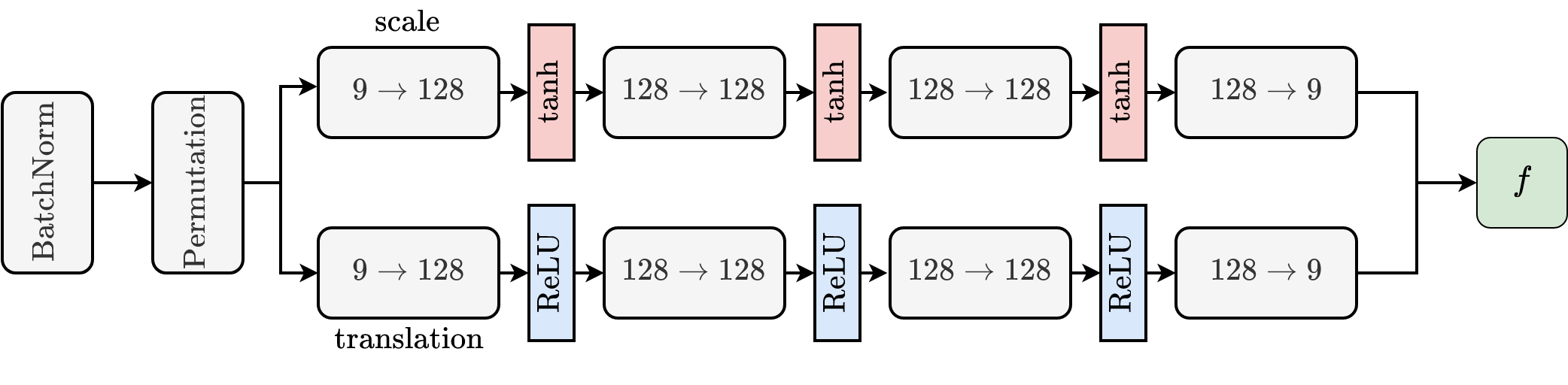
Figure 1: The building block of a coupling layer in a flow. The block consists of a coupling layer with batch normalization and learned permutations. The scaling and translation networks have the same architecture but differ in activation functions. Scaling network uses tanh functions, whereas the translation network uses ReLU functions.

The expressive power of a flow can be increased by composing multiple blocks of coupling layers, batch normalizations and permutations. The number of blocks in the flow is the main hyper-parameter of such a model. Fig. 2 shows the dependence of validation loss, i.e. the value of the loss function from Eq. (11) obtained on an validation sub-sample of the HIGGS dataset, on the number of blocks in a flow. Models with more blocks are harder to train, and show signs of over-fitting earlier. For the subsequent studies presented in this paper, one has chosen to use 10 blocks for all flow models used. A list of all other hyper-parameters is given in appendix A.

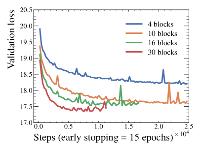
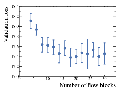
Figure 2: Validation loss as a function of training steps (epochs) and the number of flow blocks. Early stopping was employed to account for over-fitting. All other hyper-parameters were kept constant. Models were trained on $2.5\times 10^{5}$ events. The uncertainties presented in the right plot were estimated by repeated training and validation using random sampling of events. One can observe rapidly diminishing gains by using more than 10 blocks.

3.2 Autoregressive models

Using the chain rule of probability, one can rewrite any joint distribution over $D$ variables (as discussed in Ref. [24]) in the form of a product of conditional probabilities

$$p(\mathbf{z})=\prod_{i=1}^{D}p_{i}\left(\mathbf{z}_{i};c_{i}(\mathbf{z}_{<i})\right)\>,$$ (15)

where $c_{i}$ is some conditional or context on inputs. If $p_{i}\left(\mathbf{z}_{i};c_{i}(\mathbf{z}_{<i})\right)$ is conditioned on a mixture of Gaussians (MOG), one gets a RNADE model from Ref. [25]:

$$p_{i}(\mathbf{z}_{i};\mathbf{z}_{<i})=\sum_{c=1}^{C}\boldsymbol{\alpha}_{i,c}\,\mathcal{N}(\mathbf{z}_{i};\boldsymbol{\mu}_{i,c},\boldsymbol{\sigma}^{2}_{i,c})\>.$$ (16)

The mixture model parameters are calculated using a neural network that returns a vector of outputs $(\boldsymbol{\mu}_{i},\boldsymbol{\sigma}_{i},\boldsymbol{\alpha}_{i})=f_{i}(\mathbf{z}_{<i};\boldsymbol{\theta}_{i})$, as illustrated on Fig. 3.

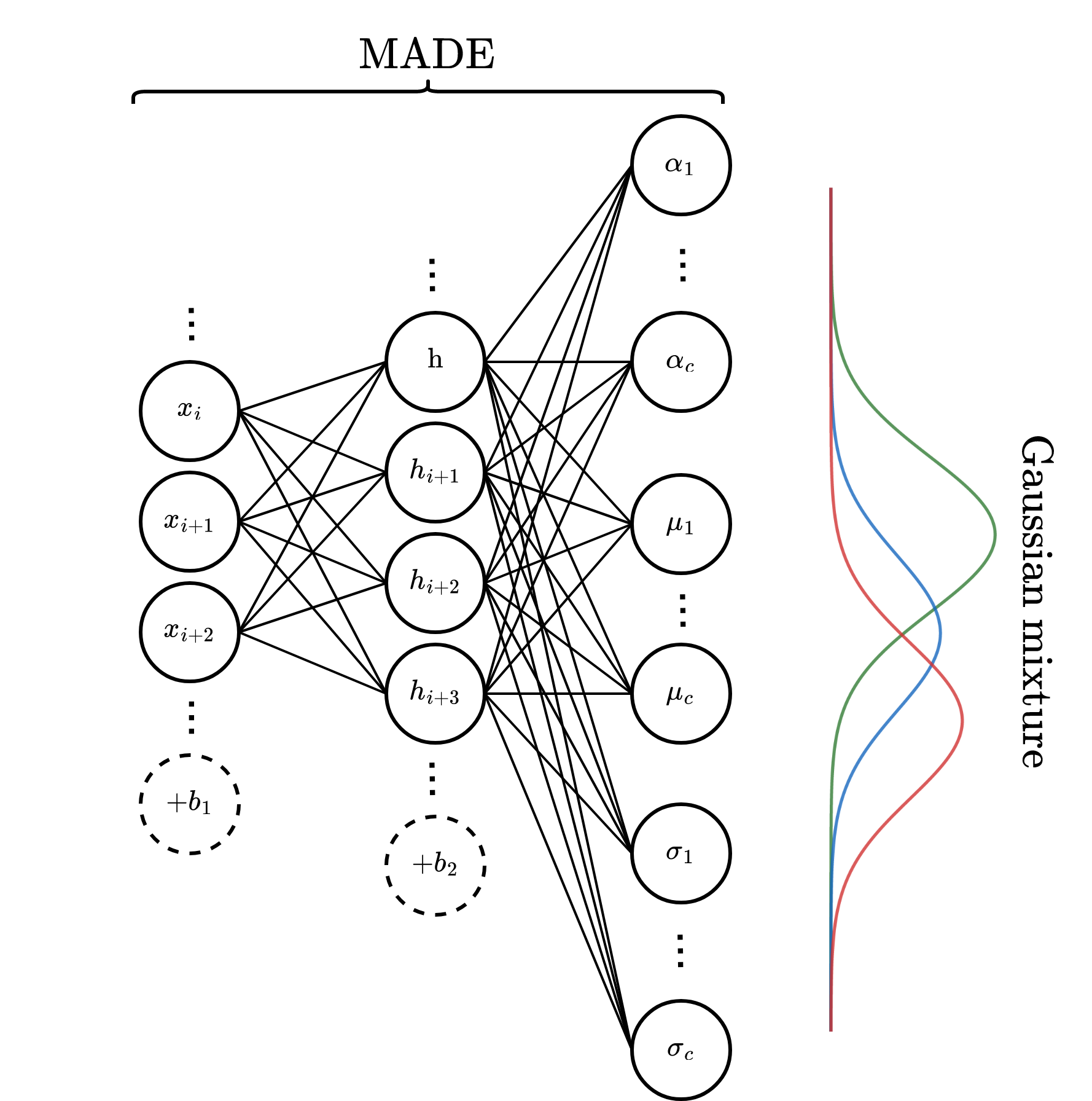
Figure 3: Mixture of Gaussians (MOG) output of a neural network implemented with MADE.

Specifically, the mixture of Gaussians parameters for the conditionals is calculated in the following sequence:

$$\mathbf{h}(\mathbf{z}) =\text{ReLU}(\mathbf{W}^{\top}\mathbf{z}+\mathbf{b})\>,$$ (17)

$$\boldsymbol{\alpha}(\mathbf{z}) =\text{softmax}(\mathbf{W}^{\top}_{\alpha}\mathbf{h}(\mathbf{z})+\mathbf{b}_{\alpha})\>,$$

$$\boldsymbol{\mu}(\mathbf{z}) =\mathbf{W}^{\top}_{\mu}\mathbf{h}(\mathbf{z})+\textbf{b}_{\mu}\>,$$

$$\boldsymbol{\sigma}(\mathbf{z}) =\text{ELU}(\mathbf{W}^{\top}_{\sigma}\mathbf{h}(\mathbf{z})+\mathbf{b}_{\sigma})+1+\varepsilon\>,$$

where $\mathbf{W}$ are the weight matrices, and $\mathbf{b}$ the bias vectors. ReLU, softmax and ELU are the activation functions. The event sampling generative step is performed simply as sampling from a Gaussian mixture. As a substantial simplification, a single neural network with $D$ inputs and $D$ outputs for each parameter vector can be used instead of using $D$ separate neural networks ($f_{i}$) for each parameter. This is done with a MADE network [26] that uses a masking strategy to ensure the autoregressive property from Eq. (15). Adding Gaussian components to a MADE network increases its flexibility. The model was proposed in Ref. [27] and is known as MADEMOG. The MADE network was implemented using residual connections from [28] as described in Ref. [29]. MADE networks can also be used as building blocks to construct a Masked Autoregressive Flow or MAF [27] by sequentially stacking MADE networks. In this case, the $i$-th conditional is given by a single Gaussian

$$p_{i}\left(\mathbf{z}_{i};c_{i}(\mathbf{z}_{<i})\right)=\mathcal{N}\left(\mathbf{z}_{i};\boldsymbol{\mu}_{i},(\exp(\boldsymbol{\sigma}_{i}))^{2}\right)\>,$$ (18)

where $\boldsymbol{\mu}_{i}=f_{\boldsymbol{\mu}_{i}}(\mathbf{z}_{<i})$ and $\boldsymbol{\sigma}_{i}=f_{\boldsymbol{\sigma}_{i}}(\mathbf{z}_{<i})$ are MADE networks. The generative sampling in this model is straightforward:

$$\mathbf{z}_{i}=\mathbf{u}_{i}\cdot\exp(\boldsymbol{\sigma}_{i})+\boldsymbol{\mu}_{i}\>,\quad\text{where}\quad\mathbf{u}_{i}\sim\mathcal{N}(0,1)$$ (19)

with a simple inverse

$$\mathbf{u}_{i}=(\mathbf{z}_{i}-\boldsymbol{\mu}_{i})\exp(-\boldsymbol{\sigma}_{i})\>,$$ (20)

which is the flow model training direction. Due to the autoregressive structure, the Jacobian is triangular (the partial derivatives $\partial x_{i}/\partial u_{j}$ are identically zero when $j>i$), hence its determinant is simply the product of its diagonal entries. One block of such a flow is presented in Fig. 4. A further option is to stack a MADEMOG on top of a MAF, which is then labelled as a MAFMADEMOG.

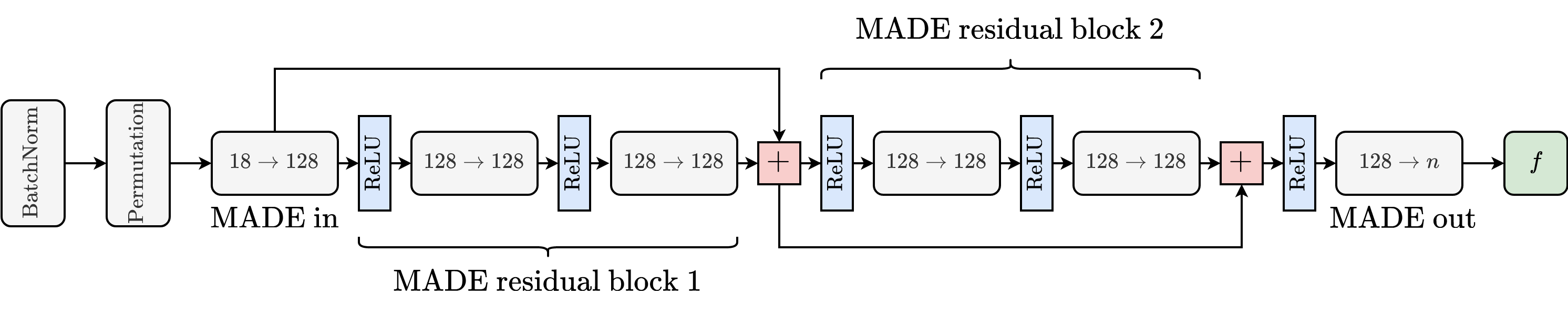
Figure 4: Block of a used MAF model. The architecture follows the one outlined in Ref. [30].

Training curves for all three types of models are shown in Fig. 5, where one can see that the MADEMOG and MAFMADEMOG achieve similar performance, in both cases significantly better than the simpler MAF. The dependence on the number of summed Gaussians is also shown, where one can see that the model performance saturates at a relatively low number of chosen Gaussian mixtures. The subsequent studies in this paper were done by choosing the number of mixture components to be the same as the number of features, i.e. 18.

3.3 Spline transformations

At the end of the flow block, one needs to choose a specific transformation $f$. So far, affine transformations of Eq. (13) and Eq. (19) were used, which were combined with sampling from Gaussian conditionals as in Eq. (16). Rather than relying on basic affine transformations, this approach can be extended to incorporate spline-based transformations.

A spline is defined as a monotonic piecewise function consisting of $K$ segments (bins). Each segment is a simple invertible function (e.g. linear or quadratic polynomial, as in Ref. [31]). In this paper, rational quadratic splines are implemented, as proposed in Ref. [30] and used by Ref. [32]. Rational quadratic functions are differentiable and are also analytically invertible, if only monotonic segments are considered. The spline parameters are then determined from neural networks in an autoregressive way. The resulting autoregressive model, replacing affine transformations of Eq. (19) and its inverse Eq. (20) with equivalent expressions for splines, is labelled as RQS in the studies of this paper. Symbolically, the generative step is thus:

$$\mathbf{z}_{i}=\text{RQS}_{i}\left(\mathbf{u}_{i},K_{i},\boldsymbol{\theta}_{i}\right),\quad\text{where}\quad\mathbf{u}_{i}\sim\mathcal{N}(0,1)$$ (21)

with an inverse

$$\mathbf{u}_{i}=\text{RQS}^{-1}_{i}\left(\mathbf{z}_{i},\mathbf{u}_{i},K_{i},\boldsymbol{\theta}_{i}\right),$$ (22)

where the $K$ represents the bin parameters and $\boldsymbol{\theta}$ denotes the remaining model (spline) parameters.

Fig. 6 shows the validation loss for different number of spline bins. The validation loss does not seem to decrease substantially with the increasing number of bins, however, as it will be shown, the quality of generated samples does, in fact, improve with more bins. For the studies performed in this paper, rational splines in 32 bins were eventually chosen.

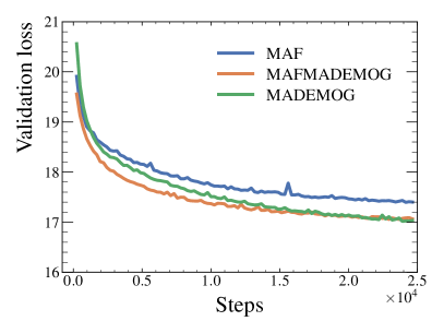
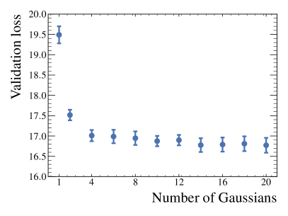
Figure 5: Validation loss as a function of training steps (epochs) for different types of models and the dependance of validation loss on the number of Gaussian components. Models were trained on $2.5\times 10^{5}$ events.

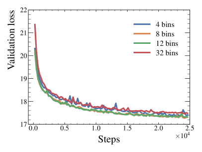
Figure 6: Validation loss as a function of training steps and number of spline bins. Models were trained on $2.5\times 10^{5}$ events.

4 Performance evaluation of the ML techniques in an analysis

After defining the appropriate evaluation data set and generative ML procedures, one can focus on the main objective of this paper, which is to systematically evaluate the performance of such tools with a finite-sized training sample in terms of requirements based on a physics analysis.

As described in the introduction, a typical particle physics analysis with the final selection and the statistical evaluation procedure uses an order of $\mathcal{O}(10)$ reconstructed kinematic observables (which are very often used to construct a final selection variable using ML techniques). The corresponding available statistics of MC signal and background events used to construct the predicted distributions of these kinematic observables, is however often of the order $\mathcal{O}(10^{5})$ events or less due to the computing resource constraints and severe filtering requirements of a new physics search. Consequently, the final kinematic region, where one searches for new physics signal, can even contain orders of magnitude fewer MC events, since one is looking for unknown new processes at the limits of achievable kinematics, which translates to “tails” of kinematic distributions.

4.1 Generated distributions of observables

Histograms of generated distributions for all three considered generative ML models, i.e. Glow, MAFMADEMOG and RQS, are shown in Fig. 7. Generated distributions are compared with their MC distributions on which the model was trained. All three models quite reliably model the original distributions, where the model with Gaussian mixtures has more success with some tails of distributions.

Histograms containing binned ratios of generated ML events and MC-simulated events are shown in Fig. 8 for the implemented models, overlaid with the shape of the normalized MC distribution (red curve) for comparison. It is evident that the deviations between the ML and MC are for all cases, except for pseudo-rapidity $\eta$, most pronounced in the tails where the event count becomes very low due to the fact that the learning algorithm did not see enough rare events in the tails of distributions and could not reproduce a reliable distribution in that region. In the case of the pseudo-rapidity distributions, the ratio deviates both at the centre and at both ends of the distribution.

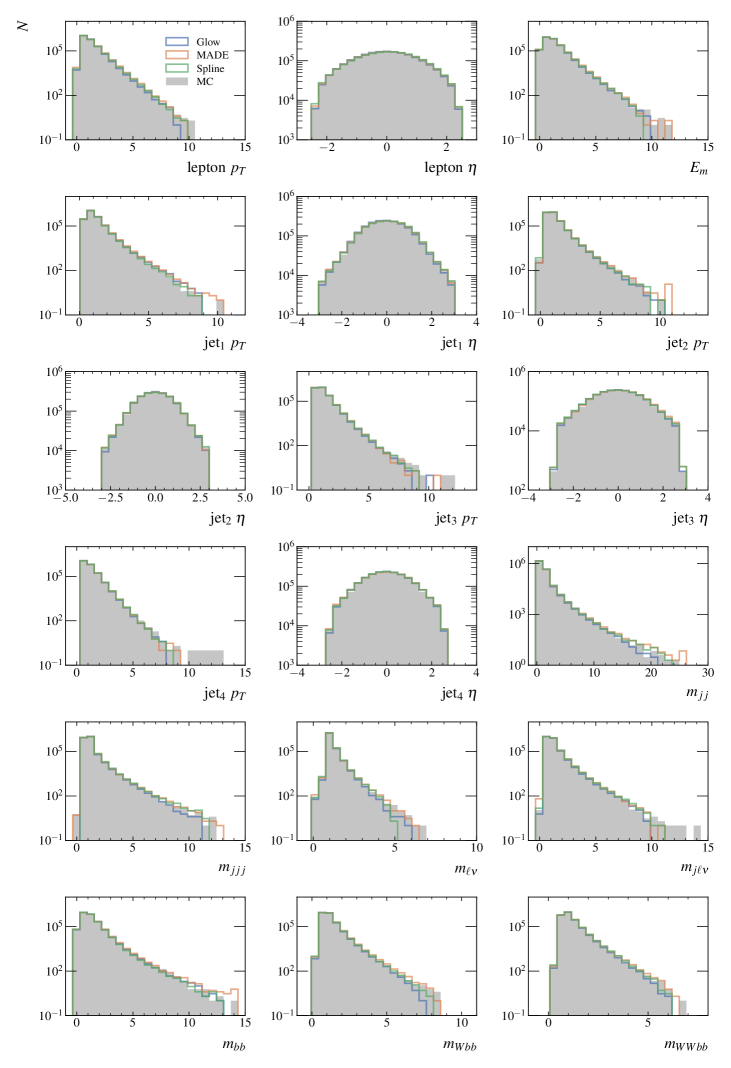
Figure 7: Distributions of $5\times 10^{6}$ events generated with models trained on $1\times 10^{6}$ events. All three models from Section 3 (Glow, MAFMADEMOG and RQS) are considered and compared with the original MC distribution in grey.

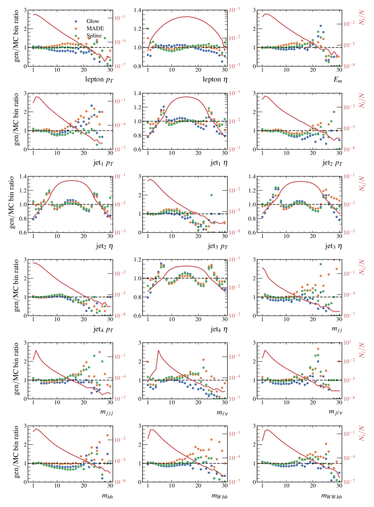
Figure 8: Histograms containing binned ratios of ML-generated events and MC-simulated events are shown for all implemented ML models. Red curves represent the normalised distributions of MC events, with the scale given in red on the right-hand side of the plots. Discrepancy between bins for MC events and ML-generated events increases in the tails of the distributions with smaller ratio $N_{i}/N$.

4.2 Simple statistical tests

The aim of this paper is to systematically define and evaluate the performance of the implemented generative ML algorithms in the context of a physics analysis. As the first step in the exploration of evaluation criteria, two of the most common statistical two-sample comparison tests are performed on the original MC events and the derived ML events from the generative procedure (trained on these MC events). When looking for possible testing algorithms, it was found that there is a notable absence of multi-variate (multi-dimensional) statistical compatibility tests that would scale to the sample sizes and dimensions expected in particle-physics analyses at the LHC.

In order to compare two samples $A$ and $B$ (MC and ML-generated data) of sizes $N$ and $M$ histogrammed in $K$ bins, a two-sample $\chi^{2}$ test described in e.g. Ref. [33] was performed. In this case, one can write $\chi^{2}$ statistics for $a_{k}$ and $b_{k}$ events from samples $A$ and $B$ in bin $k$ as

$$\chi^{2}=\sum_{k=1}^{K}\frac{(C_{1}a_{k}-C_{2}b_{k})^{2}}{a_{k}+b_{k}}$$ (23)

where

$$C_{1}=\sqrt{\frac{M}{N}}=\sqrt{\frac{\sum_{k=1}^{K}b_{k}}{\sum_{k=1}^{K}a_{k}}}\quad\text{and}\quad C_{2}=\sqrt{\frac{N}{M}}=\sqrt{\frac{\sum_{k=1}^{K}a_{k}}{\sum_{k=1}^{K}b_{k}}}$$ (24)

are weight factors. To estimate an optimal number of bins $K$, one used

$$K=\text{max}\left\{2\frac{\text{IQR}}{N^{1/3}},\>\log_{2}N+1\right\}\>,$$ (25)

where the IQR denotes the interquartile range and $N$ the sample size, combining the Freedman-Diaconis rule [34] and the Sturges’ rule [35] and which is the automatic value used in optimized automated histogramming of the NumPy package [36]. Using this rule, an arbitrary choice of binning is avoided, which could bias the observations of this paper.

The so-derived test statistic follows, approximately, a chi-square distribution with $K$ degrees of freedom, and the compatibility hypothesis is rejected if the test statistic is above the critical value $\chi_{c}(1-\alpha,K)$ at significance level of $\alpha$.

Another common test one can use is the Kolmogorov-Smirnov (KS) test (see e.g. Ref. [33, 37] for further discussion). In the case of two samples, the distance $D$ measured between two empirical distributions is calculated as the supremum of the set of distances between the distribution functions (cumulants, ECDF) $S_{1,2}$ of the two samples.

$$D=\underset{x}{\text{sup}}|S_{1}(x)-S_{2}(x)|\>.$$ (26)

The compatibility test is again performed using a critical value $\text{KS}_{c}(\alpha)$ at significance level $\alpha$.

Both tests require one-dimensional distributions. One can thus either apply the tests feature-wise (for each observable independently), or use a method to reduce the dimensionality of our dataset to one dimension. In this paper, a classification neural network was used to achieve this, which closely matches what would also be done in an actual physics analysis as the final filtering (event selection) step and exploits the fact that there are both background and new physics signal contributions available in the HIGGS dataset, identifiable by a binary label. The input to the classifier is a vector of observables and a label (1 for signal events and 0 for background events). The output score value is a scalar that can be used to distinguish background from signal. Consequently, a transformation from a vector to a scalar was obtained, which one can use to reduce the dimensionality of our data. As a classifier, a simple neural network with an unbound output, and an MSE loss function was used. The test accuracy of such a network was estimated to be about $75\%$.

An example of dimensionality reduction with a classifier is shown in Fig. 9 for both signal and background contributions. One can observe that the performance of the ML-generated sample is quite close to the original MC sample.

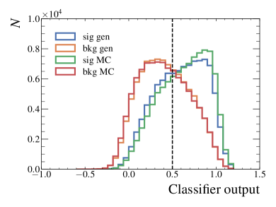
Figure 9: Dimensionality reduction with a neural network classifier, resulting in a scalar score value. Both MC-simulated and ML-generated distributions using the Glow method are shown.

4.3 Test scaling with increasing number of generated events

The critical value $\chi_{c}(1-\alpha,K)$ of the $\chi^{2}$ test depends on the number of bins $K$ and thus indirectly, using the automated rule of Eq. (25), also on the event statistics, whereas the critical value $\text{KS}_{c}(\alpha)$ of the Kolmogorov-Smirnov test depends on the number of events directly. Consequently, since the generative ML model is an approximation of the MC process, one can expect that at a certain number of ML-generated events, the statistical tests will necessarily fail as a result of the increasing deviation between the growth of the critical value and the test statistics. The value of $N$, at which the divergence between the two values and the subsequent test failure occurs, is determined by the quality of our generative model.

This scaling of the critical values and the test scores as a function of the number of events $N$ is shown in Fig. 10 for the classifier-reduced data dimensionality. The tests show that a statistically acceptable value for the number of events is around $10^{5}$. Above this number of events, however, the test value and the critical value start to diverge.

This can in fact be interpreted as an important observation, namely that the advanced generative ML algorithms exhaust their matching power to the MC at $\mathcal{O}(10^{5})$ events, which thus gives a measure of the training sample statistics that is appropriate (or required) for these ML algorithms. Since, as already stated, the available MC samples of physical processes at the LHC are typically of the order of $\mathcal{O}(10^{5})$ events, which means that it is in fact feasible to construct generative ML procedures using such training samples.

Another point to stress in the interpretation of these results is that these simple tests are likely overly strict when comparing the predictive precision of the ML-generated distributions. In other words, even the best representative ML generative algorithm would never be good enough to extend the simulated statistics by orders of magnitude, as is the goal of the ML generative approaches in the existing particle physics studies including in this paper. Instead, we should consider what approximation is good enough in terms of the achievable precision of an analysis, involving limited data statistics as well as a plethora of measurement systematic uncertainties and specific statistical analysis procedures, which are further explored in the following sections of this paper.

To gain further insight, one can also perform both tests for each generated observable distribution separately, as shown in Fig. 11. It is evident that some observables get modeled better than others, depending on the sensitivity region of a specific test. Results depend on the model used, and it is clear that the performance of autoregressive methods is significantly better than the simpler alternatives.

The impact of the number of training events used in the range of $\mathcal{O}(10^{4}-10^{6})$ is shown in Fig. 12. The figure shows the convergence of the ratios of the test statistics and their corresponding critical values for a fixed size of ML data generated by models trained on different number of MC events. The improvement with larger training sets is evident. As already stated, the increase in the training (MC) sample size nonetheless has a diminishing return because, at some point, the limit saturates as the ML model exhausts its matching capacity (i.e. learning potential) to the MC sample. The impact of the increase in the training dataset size is, in fact, most evident in the better generation of events in the tails of distributions, where the poorest statistics is available, as also evident from Figs 7 and 8.

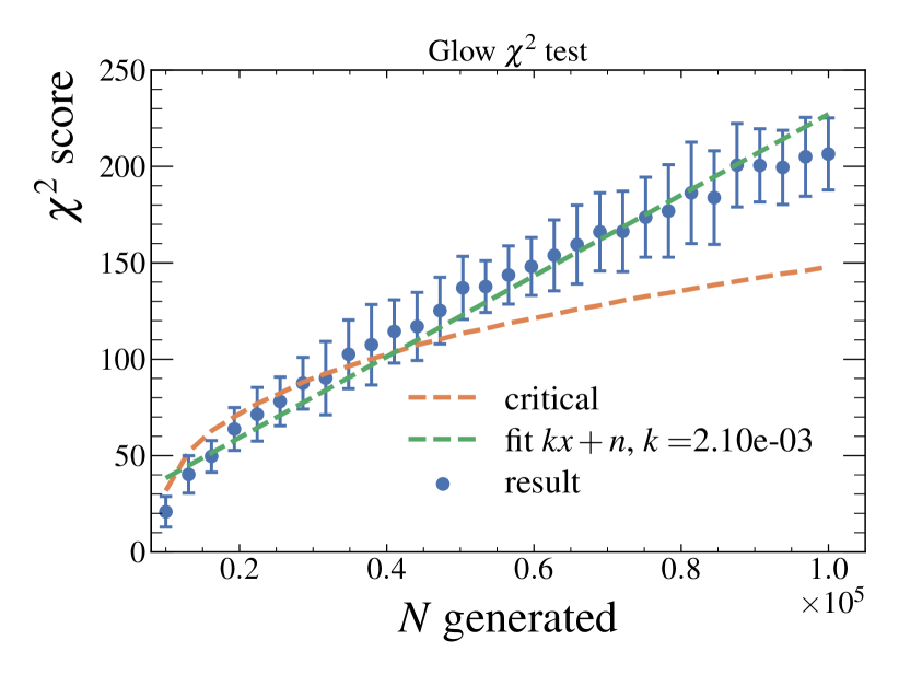
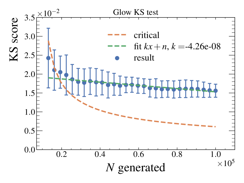
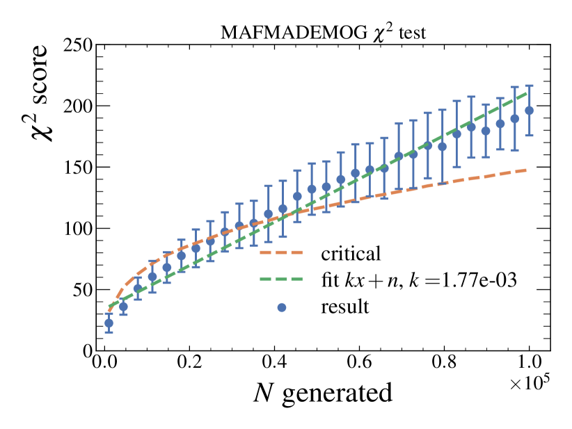
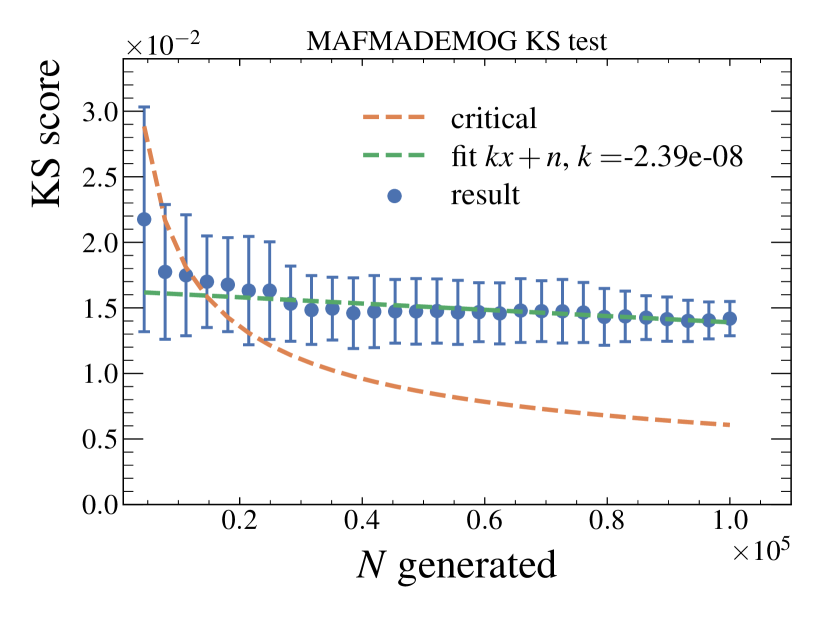
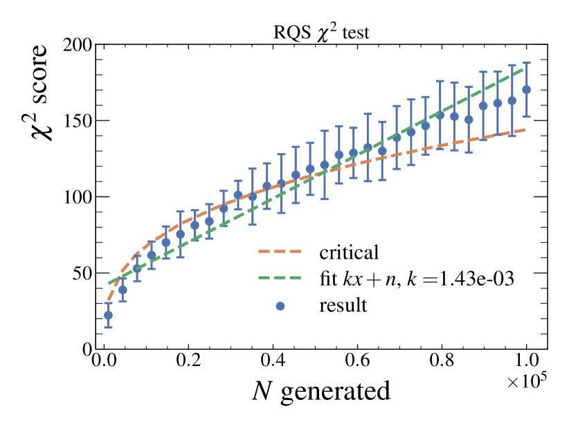
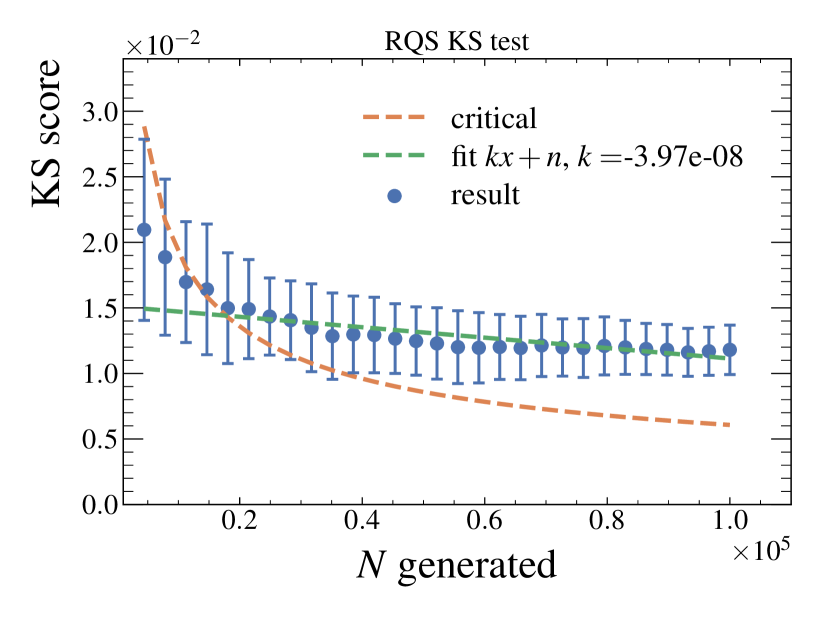
Figure 10: Performance of the two-sample tests using $\chi^{2}$ (left) and the Kolmogorov-Smirnov test (right) is shown for different implementations of the generative ML algorithms using Glow (top) MAFMADEMOG (middle) and RQS (bottom) approaches as described in Section 3. The plots show the test score as a function of the ML-generated number of events $N$ (error bars) compared to the critical value of the test (red curve) at $\alpha=0.05$. The dimensionality of the generated and MC data was reduced using a neural network classifier, and the distributions of events w.r.t. the classifier score were used in the tests. In addition, a linear fit (green line) has been performed on the test scores to approximately show the divergence with increasing $N$.

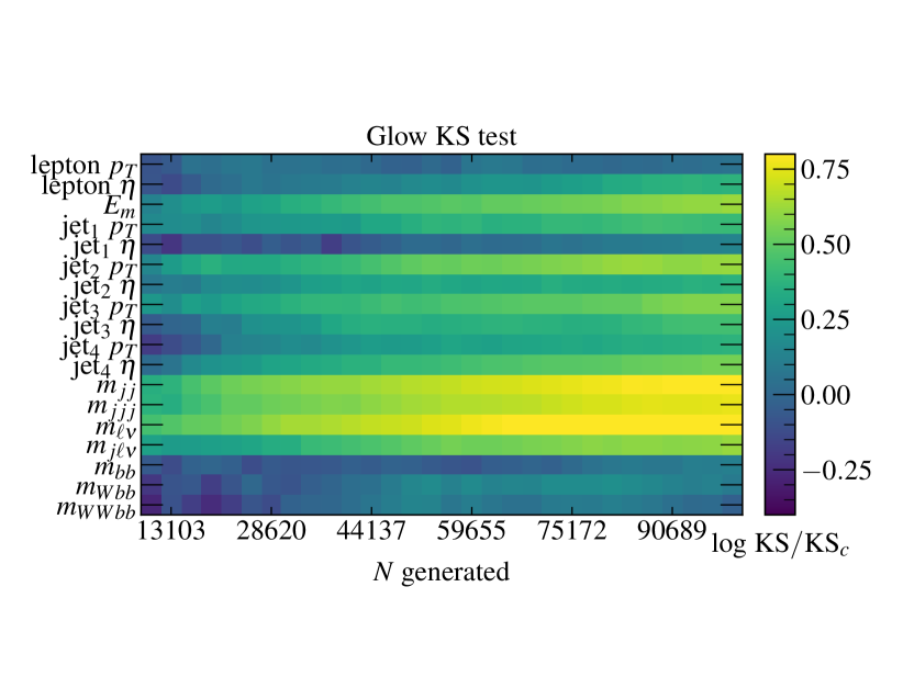
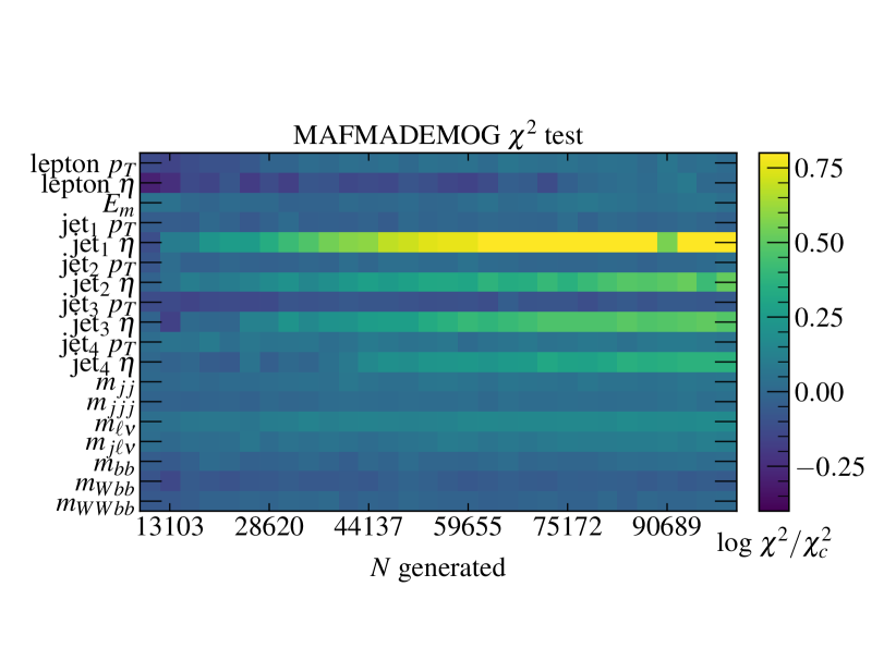
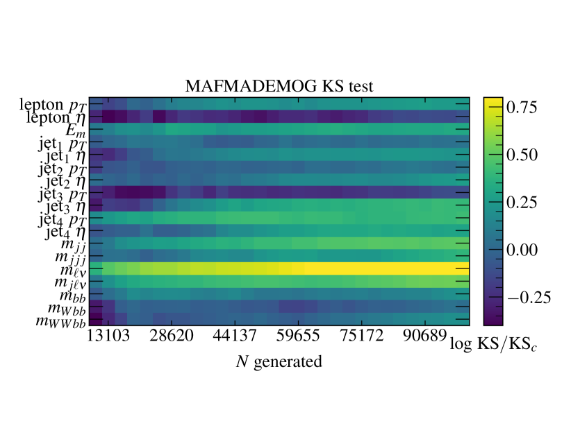
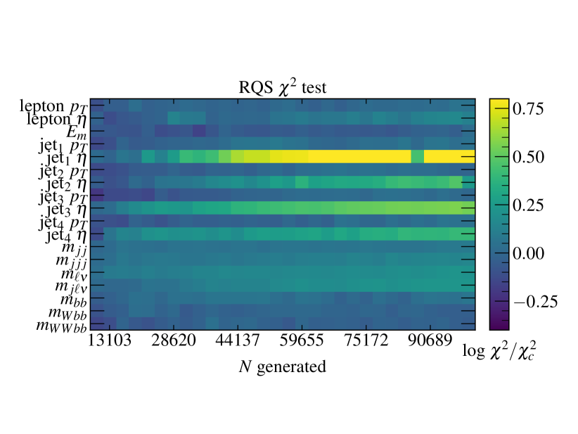
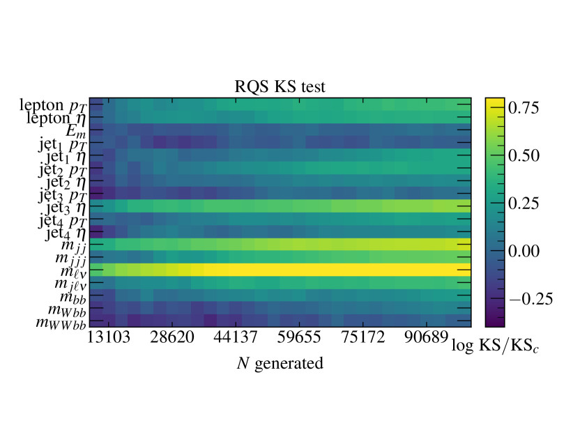
Figure 11: Ratios of test results and critical values for each generated feature distribution.

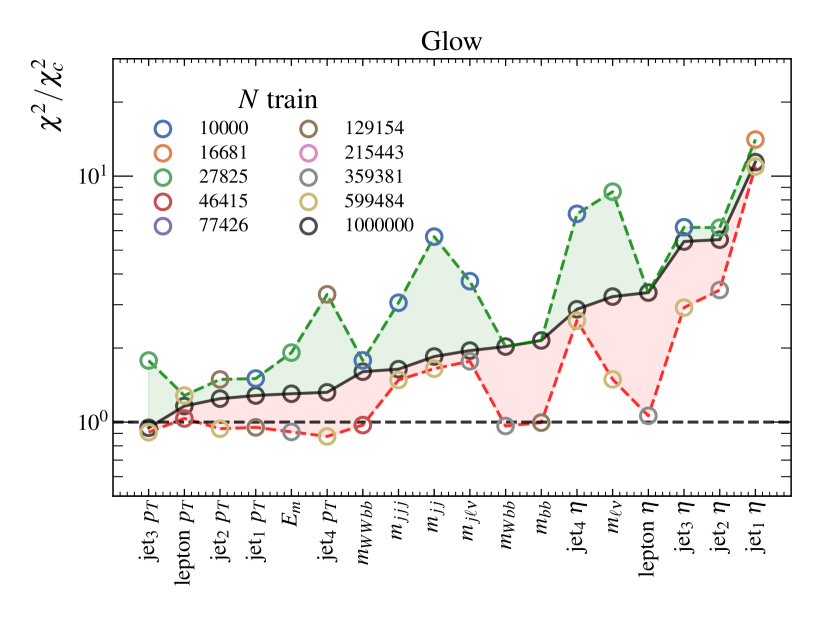
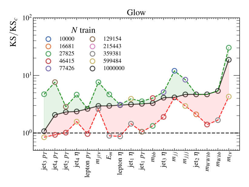
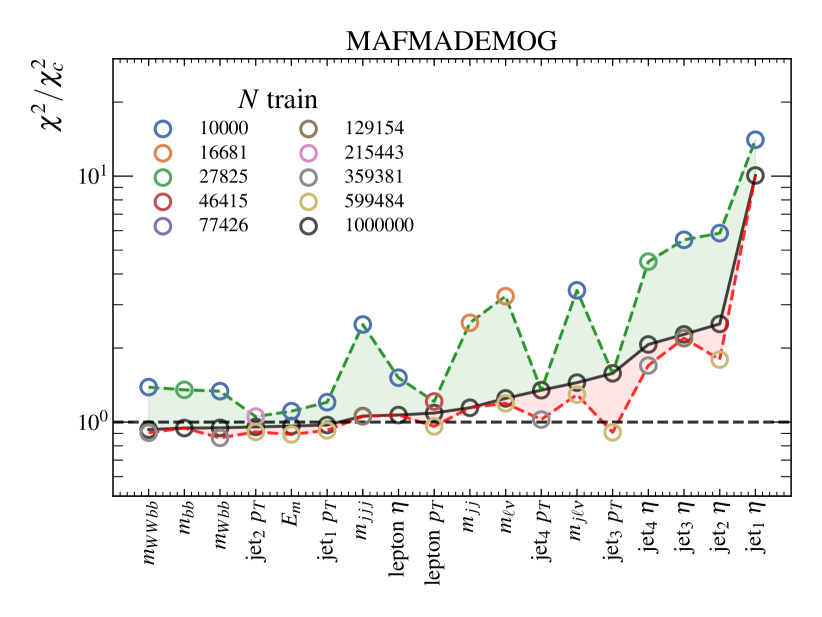
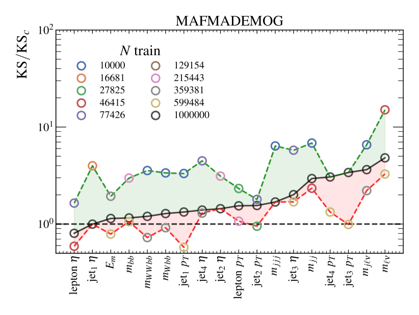
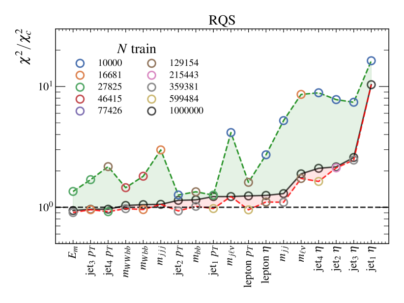
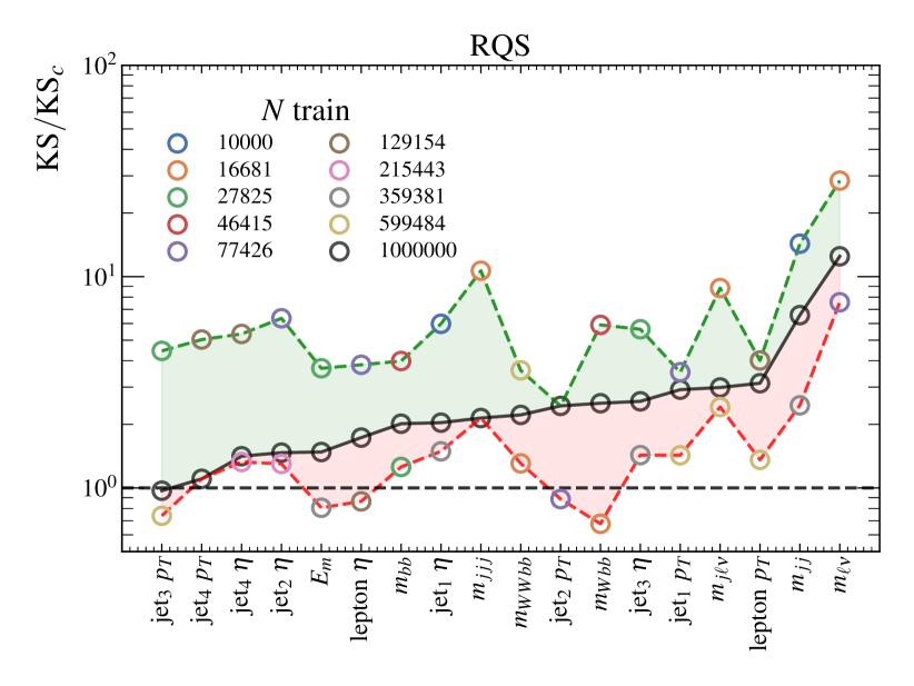
Figure 12: Ratios of test statistic and its critical value for data generated by models trained on different number of events. For every size $N$ of the training set, a newly initialized model was used. Test values were calculated 10 times for $10^{5}$ generated events and then averaged for every feature. In order to obtain the uncertainty bands, the extreme values obtained in all scenarios were selected.

5 ML performance evaluation in a physics analysis

In order to provide a relevant quantitative evaluation of the impact of the imperfect agreement of ML-generated distributions with the MC-generated ones in an analysis environment, a simplified analysis setup was constructed that matches the statistical analysis of a new physics search in an LHC experiment. In this setup, the HIGGS sample was used for training the ML-generative algorithms for both signal and background. In the following studies, the MADEMOG model trained on the HIGGS dataset was used to generate the new samples.

In order to emulate a typical analysis procedure in an LHC experiment, a further step was introduced, namely the ML generative algorithm was trained and applied on the full HIGGS sample (signal and background training was performed separately), while the statistical analysis studies were done after an additional cut on the classifier from Figure 9 at the score value of 0.50 . This is intended to match the standard analysis approach, where first a relatively simple baseline selection is applied on the data and MC samples as the first stage of analysis optimisation, and which approximately matches the agreement of kinematics of the signal and background in the HIGGS sample used in this study. After the baseline selection, a current LHC analysis then uses the MC samples to train an advanced classifier (usually ML-based approach is used) to perform a final data selection to achieve an optimal signal-to-background separation. The simulated samples in new physics searches tend to have quite low statistics after the final selection, too low to be usable to effectively train a ML generative procedure.

Consequently, the same steps were also taken in this paper, which is an innovative implementation of the study presented in this paper. The procedure can be summarised as follows:

1. train a generative model on full MC samples and generate large datasets of new events using it,

2. apply the baseline selection on the generated ML samples using a neural network classifier,

3. normalise the generated ML samples to match the data sample after the baseline selection,

4. perform the statistical analysis.

By introducing a (ML) classifier cut, one can also see how well the multi-dimensional generation of correlated variables is in fact performing. As a further insight from a different perspective, without final cuts, each relevant kinematic distribution can just be modelled (smoothed) independently, without a need for a generative procedure.

As one can observe in Figure 13, good agreement is preserved between the MC and ML samples, demonstrating that the variable correlations are adequately modelled and that the ML generative approach is thus usable for such an analysis approach.

In order to provide representative event yields, the background normalisation of the binned distributions used in statistical analysis after the final selection was set to yield $B=10^{3}$ events at an integrated luminosity of $L=$100 fb^-1, which matches the order of magnitude of a typical background contribution in the final data selection of a Run 2 new physics search at the LHC. For further studies with varying luminosity, the background yield was evaluated in the range $B\in[10^{3},10^{4}]$, corresponding to a luminosity increase up to one order of magnitude ($L\in[100~{}\text{fb}^{-1},1000~{}\text{fb}^{-1}]$). The signal yield ($S$) fraction, denoted $\alpha=S/B$, was set to have a value of up to 10% of the background yield in the performed tests, whereby the signal normalisation was varied in this range in the sensitivity studies presented below. An inclusive relative systematic uncertainty ($\beta$), which in a real analysis would comprise both theoretical and experimental uncertainties, was set to $\beta=$10%, excluding the systematic uncertainty due to finite simulated sample statistics, which is the focus of this study and is being treated separately and has the expected total Poisson-like $\sim\sqrt{N}$ dependence on the number of generated events for the normalised background prediction, translating into the appropriate multinomial uncertainties in binned distributions.

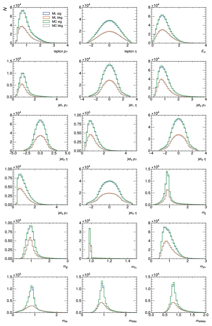
Figure 13: Cuts on the classifier from Figure 9 at an output score of 0.50 .

The data prediction was constructed by adding the MC-simulated samples of background and signal with a chosen signal content, giving a so-called Asimov dataset, which perfectly matches the MC-samples and is often used in the performance validation of a statistical analysis in an LHC experiment. For the purpose of the studies in this paper, the MC-simulated background is then replaced with ML-generated samples, whereby the ML procedure was trained on these MC-samples.

The signal prediction is retained as the MC one because in LHC analyses, the signal simulation, which generally has a comparatively small number of generated events, is typically not as much of an issue as the background. The final analysis selection is centred around the signal prediction, retaining most of the signal statistics while only selecting the low-statistics tails of the background samples. This aims to provide a good measure of the quality of the ML approach in a LHC analysis environment - ideally the results after this replacement would still perfectly match the results of the original MC setup on the Asimov data set, however, an agreement within the joint statistical and systematic uncertainty is still deemed as acceptable, and thus a successful ML implementation.

The achieved statistical agreement certainly depends on the luminosity, i.e. data statistics, assuming a constant presence of a fixed total systematic uncertainty, which then translates into a requirement on the quality of ML-generated samples, assuming that an arbitrarily large statistics (size) of these ML-generated samples is easily achievable.

In addition to a standard upper-limit and $p$-value evaluation in this analysis setup, a sequence of tests proposed in Ref. [38] in terms of spurious signal evaluation was performed to give a relevant quantitative evaluation of the impact of ML-generated samples.

With the aim of closely matching a typical statistical analysis as done in LHC experiments, the HistFactory model from the pyhf [39, 40] statistical tool was used, and different standard procedures of evaluation of the agreement between data and simulation predictions were implemented (profile likelihood calculation, upper limit estimation, background-only hypothesis probability etc…). The statistical analysis was performed using two different possibilities for choosing the optimal variable, resulting in a binned distribution w.r.t. the $m_{bb}$ in the first case and classifier output observable in the second case, which aims to give an optimal separation between the shape of the background and signal predictions. In the statistical analysis, the signal presence is evaluated by using a scaling factor $\mu$ (signal strength) of the predicted signal normalisation. Statistical error scale factors $\boldsymbol{\gamma}=\{\gamma_{i}\}$ are used to model the uncertainty in the bins due to the limited statistics of (ML-)simulated samples. By using the fast ML event generation, one aims to push this uncertainty to negligible values, as is indeed done in the study presented below. As already stated, the simulated predictions are given an additional overall relative uncertainty of $\beta=$10% in each bin to model the systematic uncertainty contribution as $\boldsymbol{\beta}=\{\beta_{i}\}$. In the likelihood calculation, the parameters $\boldsymbol{\gamma}$ and $\boldsymbol{\beta}$ are modelled as nuisance parameters in addition to $\mu$ as the main parameter of the likelihood fit.

The binned distributions of samples used in this statistical analysis, together with the injected uncertainties, are shown in Figure 14 for the two relevant observables. One can see that the agreement between the Asimov data and the simulation prediction using the ML-generated background sample is well within the simulated sample uncertainties, which is an encouraging starting point for a detailed analysis.

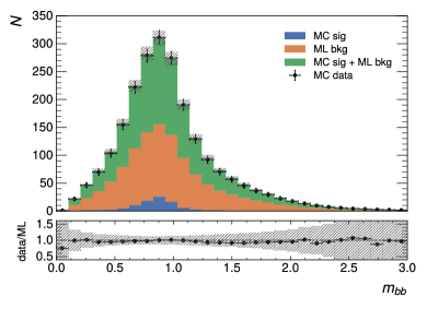
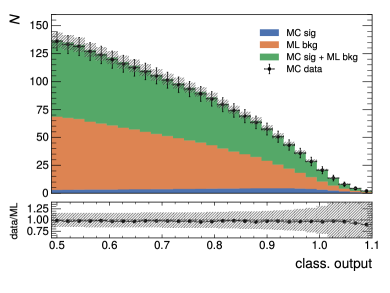
Figure 14: $m_{bb}$ and classifier distributions after the classifier cut. The “MC data” (crosses) represents the Asimov data set composed from MC signal and background prediction and matches quite well the combined MC signal (blue) and ML background (orange) prediction (green histogram).

In more detail, the likelihood is defined as the product over all bins of the Poisson probability to observe $N_{i}$ events in a particular bin $i$:

$$L_{\text{phys}}(\text{data}\,|\,\mu)=L_{\text{phys}}(\mu)$$ (27)

$$=\prod_{i\in\text{bins}}\text{Pois}(N_{i}\,|\,\mu S_{i}+B_{i})$$

$$=\prod_{i\in\text{bins}}\frac{(\mu S_{i}+B_{i})^{N_{i}}}{N_{i}!}e^{-(\mu S_{i}+B_{i})},$$

where $S_{i}$ and $B_{i}$ are the expected signal and background yields, respectively. As already stated, the main parameter of interest is the signal strength, denoted as $\mu$.

The systematic uncertainties are included in the likelihood via a set of nuisance parameters (NP), denoted as $\boldsymbol{\theta}=(\boldsymbol{\beta},\boldsymbol{\gamma})$, that modify the expected background yield, i.e. $\{B_{i}\}\to\{B_{i}(\boldsymbol{\theta})\}$. The overall relative systematic uncertainties $\beta_{i}$ can be encoded into Gaussian functions and subsequently into an auxiliary likelihood function $L_{\text{aux}}(\boldsymbol{\beta})$, while the uncertainties on the background predictions due to the limited number of simulated events are accounted for in the likelihood function considering Poisson terms

$$L_{\text{stat}}(\boldsymbol{\gamma})=\prod_{i\in\text{bins}}\frac{(\gamma_{i}B_{i})^{B_{i}}e^{-\gamma_{i}B_{i}}}{\Gamma(B_{i})},$$ (28)

where $\Gamma$ is the Gamma function.

The final profile likelihood function can finally be defined as a product of three likelihoods

$$L(\mu,\boldsymbol{\theta})=L_{\text{phys}}(\mu)\cdot L_{\text{aux}}(\boldsymbol{\beta})\cdot L_{\text{stat}}(\boldsymbol{\gamma}).$$ (29)

A likelihood fit using this likelihood is then performed to determine the value of $\mu$ and its uncertainty, as well as the nuisance parameters. The estimates of $\mu$ and $\boldsymbol{\theta}$ are obtained as the values of the parameters that maximise the likelihood function $L(\mu,\boldsymbol{\theta})$ or, equivalently, minimise $-\!\ln L(\mu,\boldsymbol{\theta})$.

This profile likelihood function is also used to construct statistical tests of w.r.t. the hypothesised value of $\mu$. A profile likelihood ratio, $\lambda(\mu)$, is defined as

$$\lambda(\mu)=\frac{L(\mu,\hat{\hat{\boldsymbol{\theta}}}(\mu))}{L(\hat{\mu},\hat{\boldsymbol{\theta}})},$$ (30)

where $\hat{\mu}$ and $\hat{\boldsymbol{\theta}}$ are the parameters that maximise the overall likelihood, and $\hat{\hat{\boldsymbol{\theta}}}$ are the NP values that maximise the likelihood for a particular value of $\mu$. The test statistic is then defined as $q_{\mu}=-2\ln\lambda(\mu)$, for which the lower values indicate better compatibility between the data and the hypothesised value of $\mu$. The test statistic is used to calculate a p-value that quantifies the agreement

$$p_{\mu}=\int_{q_{\mu}^{\text{obs}}}^{\infty}f(q_{\mu}\,|\,\mu)\,\text{d}q_{\mu},$$ (31)

where $q_{\mu}^{\text{obs}}$ is the value of test statistics observed in the data, and $f(q_{\mu}\,|\,\mu)$ is the probability density function of the test statistic $q_{\mu}$ under the signal strength assumption, $\mu$. The $p$-value can be expressed in units of Gaussian standard deviations $Z=\Phi^{-1}(1-p)$, where $\Phi^{-1}$ is the inverse Gaussian CDF. The rejection of the background-only hypothesis ($\mu=0$) with a significance of at least $Z=5$ (corresponding to $p_{0}=2.87\times 10^{-7}$) is considered a discovery.

A test statistic used in this analysis is the one for the positive signal discovery in which the background-only hypothesis with $\mu=0$ is tested. If the data is compatible with the background-only hypothesis, the nominator and the denominator of the test statistic, $q_{0}=-2\ln\lambda(\mu=0)$, are similar. Then, $q_{0}$ is close to 0, and $p_{0}$ value is 0.5. For this scenario, upper limits on the signal strength are derived at a CL=95% confidence level using the $\text{CL}_{\text{s}}$ method [41], for which both the signal plus background, $p_{S+B}$, and background-only, $p_{B}$, $p$-values need to be calculated. For a given set of signal masses or branching ratios, the signal hypothesis is tested for several values of $\mu$. The final confidence level $\text{CL}_{\text{s}}$ is computed as the ratio $\text{CL}_{\text{s}}\equiv\frac{p_{S+B}}{1-p_{B}}$, which excludes a signal hypothesis at CL=95% when giving a value below 5%.

5.1 Results of statistical tests

Examples of distributions obtained from profile likelihood fit results to the Asimov data described above are shown on Figure 15 for different variable selections. One can observe a very nice agreement between the fitted prediction and Asimov data, well within the uncertainty band. The improvement of the agreement between the Asimov data and prediction using ML-generated background, after the likelihood fit to the distribution of the indicated observable, is shown in Figure 16.

In Figure 17 the reproduction of the expected value of the signal strength is shown w.r.t. the increase in integrated luminosity. The signal strength is scaled to the value of the injected signal fraction $\alpha$, giving $\mu=\alpha$ as the ideal outcome. An impact of the size (fraction) $\alpha$ of the injected signal with respect to the background and the performance of the likelihood fit w.r.t. the increase in integrated luminosity is also shown. One can observe that for decreasing signal presence (lower $\alpha$ values) the performance of the fit is progressively worse, leading to a bias even with increasing integrated luminosity. The (biased) values are still within the uncertainty, as shown on Figure 19, for the difference $\mu-\alpha$, but it is of course clear that background mis-modelling, present when using ML-generated background, leads to sensitivity loss and possible biases in an analysis with relatively tiny signal presence. Figure 18 gives a nice quantitative measure of this.

The discrepancy between the injected and estimated signal in the final analysis fit can also be interpreted as the presence of a spurious signal. Its evaluation is a common approach in LHC analyses. An example of the spurious signal presence in this analysis is given in Figure 19 as a function of integrated luminosity. One can observe that using the ML-generated background indeed gives a non-zero spurious signal content as a bias, which is however well within the estimated total uncertainty of the measurement across the relevant luminosity range. The value of the bias depends on the variable used in the fitting scenario.

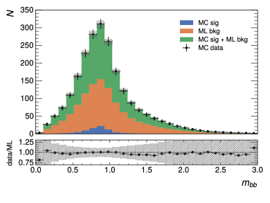
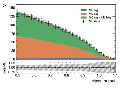
Figure 15: Post-fit distributions for profile likelihood fits to the $m_{bb}$ or the classifier output variable.

Using the derived profile likelihood in a test statistic to determine the signal and background hypothesis probabilities (p-values in LHC jargon) and the eventual CL${}_{\text{s}}$ value, as described above, is shown in Figure 20 as a function of the injected signal fraction $\alpha$. Results for the ideal scenario, using only the MC simulated samples, which identically match the Asimov dataset, are shown for comparison with the ML-generated background results. One can see that the relevant observables, in particular CL${}_{\text{s}}$, converge nicely with increasing signal presence, while there is a discrepancy when the signal presence is diminishing, which agrees with observations from Figure 17.

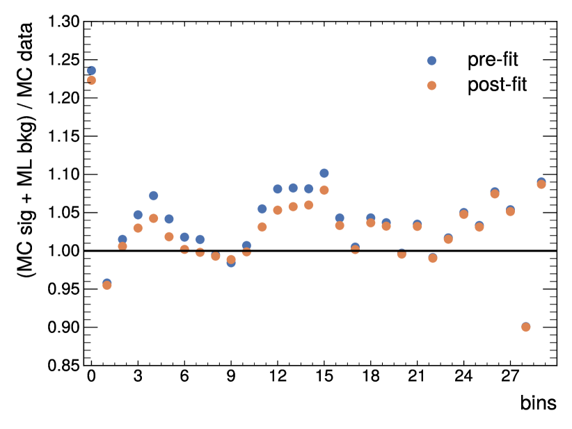
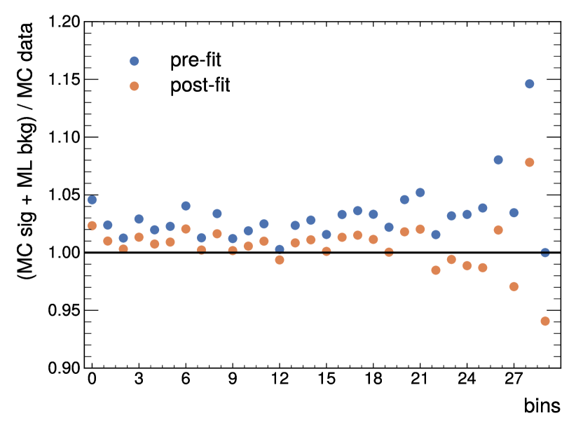
Figure 16: Ratios between pre-fit and post-fit results for both scenarios ($m_{bb}$ and classifier output).

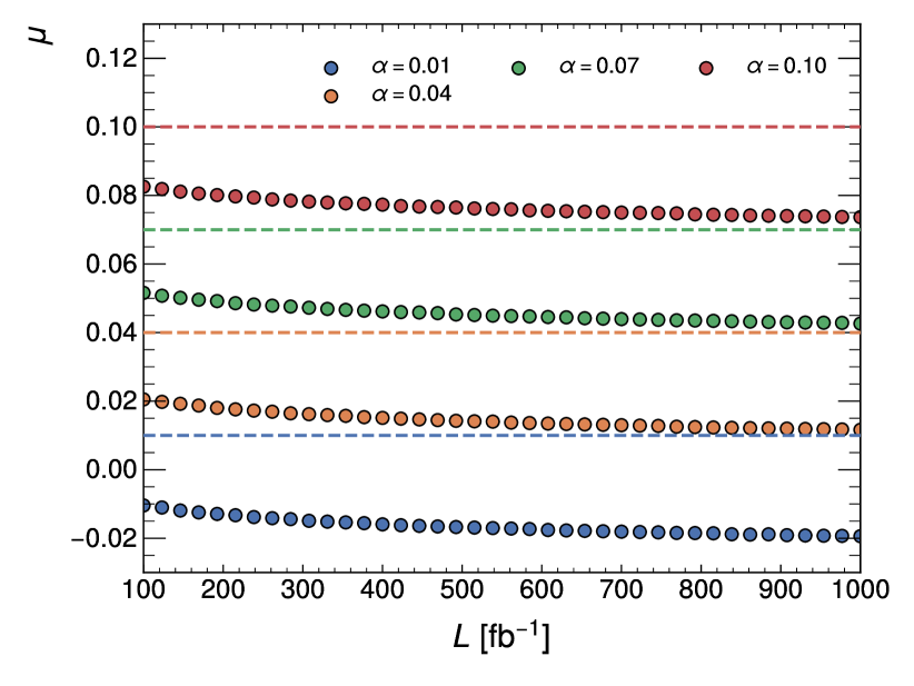
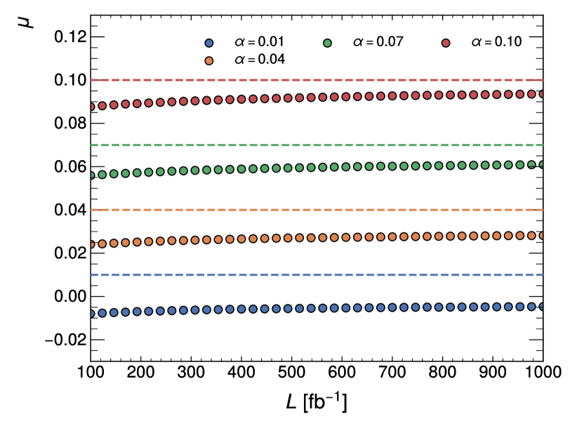
Figure 17: Fitted signal strength $\mu$ as a function of integrated luminosity $L$ for both scenarios ($m_{bb}$ and classifier output) of likelihood fit at different values of $\alpha=S/B$.

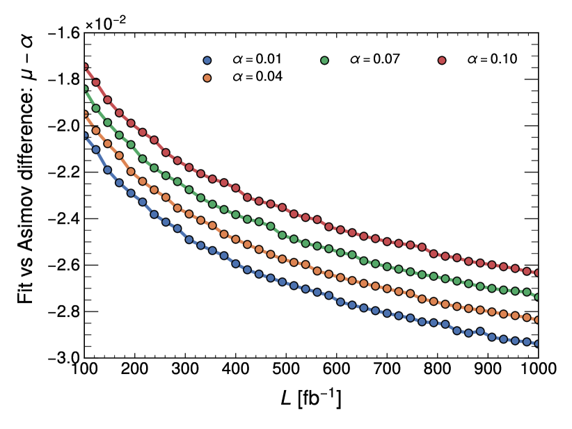
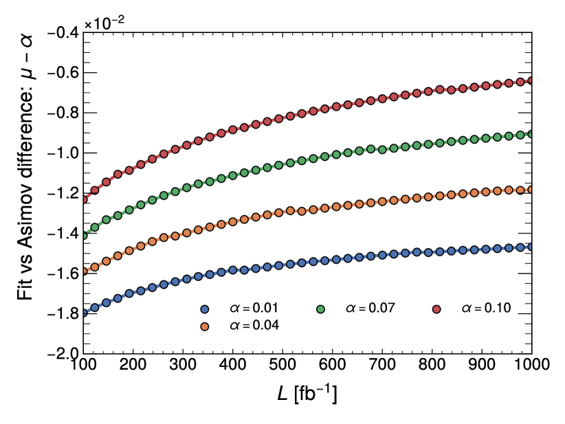
Figure 18: Difference of fitted signal strength $\mu$ and Asimov $\alpha$ value as a function of integrated luminosity $L$ for both scenarios ($m_{bb}$ and classifier output).

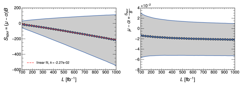
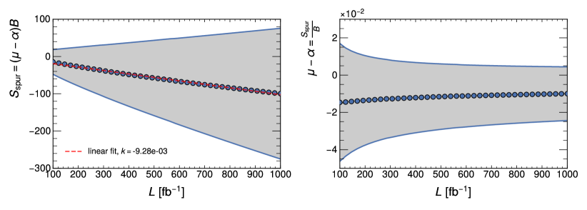
Figure 19: Estimated spurious signal as a function of integrated luminosity $L$ for both scenarios ($m_{bb}$ and classifier output) of likelihood fits with $\alpha=0.1$ from Fig. 17.

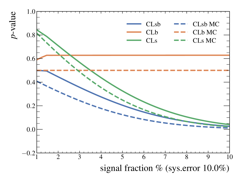
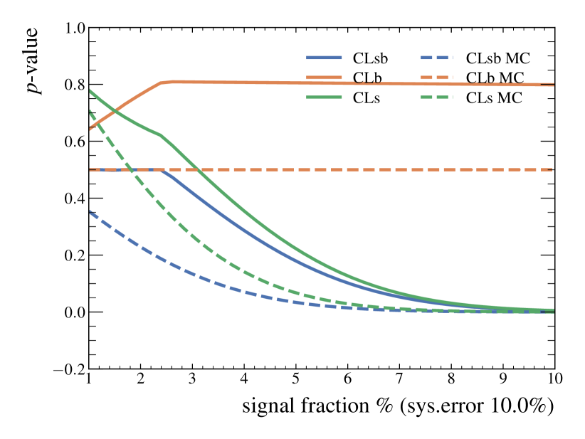
Figure 20: Estimated $p$-values for signal and background , background and CL${}_{\text{s}}$ for both scenarios ($m_{bb}$ and classifier output) at different values of $\alpha=S/B$.

6 Upper limits

As the final step in this physics analysis study, one aims to evaluate the upper limits on the signal strength, together with the uncertainty estimates using the profile-likelihood-based test statistics, as is done in LHC analyses. The dependence of the extracted upper limit as a function of integrated luminosity is shown in figures Fig. 21 and Fig. 22 for different values of injected signal fraction $\alpha$ and the two fitting scenarios. Again, the ideal (reference) scenario, using the MC simulated samples both for Asimov data construction and simulated predictions is used as a reference, and is in the figures shown together with the derived uncertainty bands. One can observe that the shifts in upper limit estimation are on a scale compatible with the estimated uncertainties for the reference scenario.

From these results it is evident that the ML-generated samples can indeed be used in a physics analysis as a surrogate model for the background prediction. However, to further minimize the impact of the background ML mis-modelling, one would need to work on implementing techniques that go even beyond the current commercial state-of-the-art approaches used in this paper, and to understand how to optimally adapt them for this use case in high energy physics.

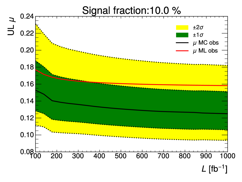
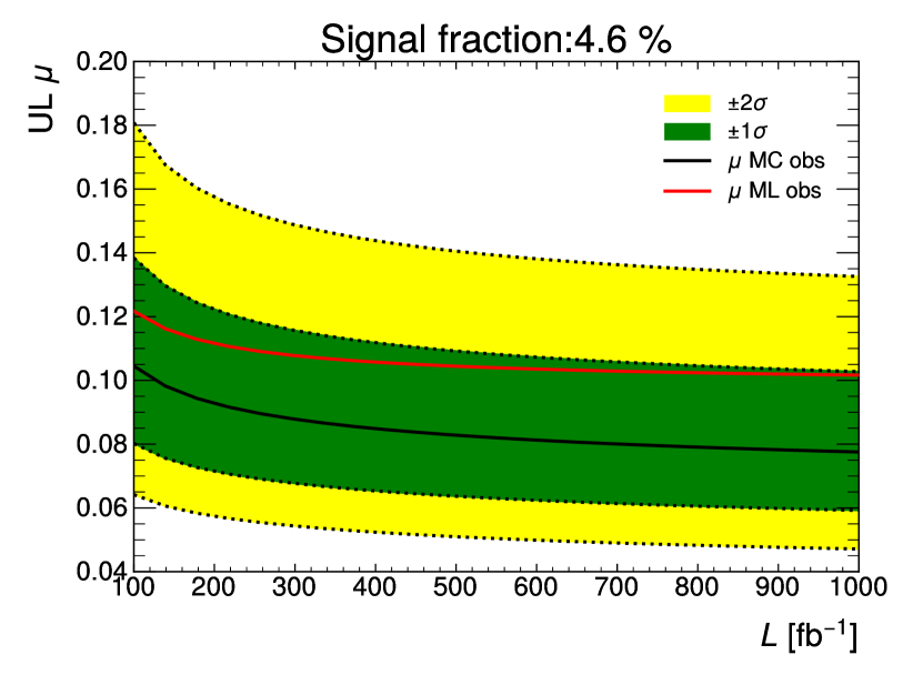
Figure 21: Upper limits on the signal strength $\mu$ as a function of integrated luminosity $L$ for the likelihood fit to the $m_{bb}$ distribution.

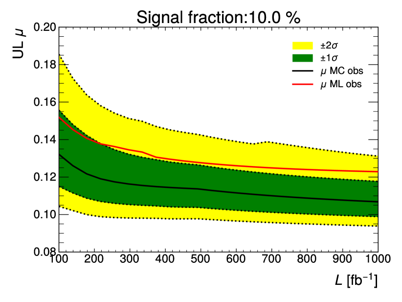
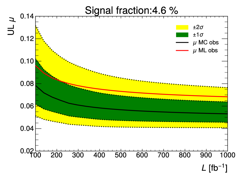
Figure 22: Upper limits on the signal strength ($\mu$) as a function of integrated luminosity $L$ for the likelihood fit to the classifier output distribution.

7 Discussion and outlook

The paper investigates the possibility of using normalizing flows for analysis-specific ML-based generation of events used by the final stage of a given particle physics analysis, where the state-of-the-art generative ML algorithms are trained on the available MC-simulated samples. The extended custom event samples can thus serve to extend the MC statistics, thereby minimizing the analysis uncertainty due to the statistics limitations of MC events or, equivalently, to smooth and minimize the uncertainties on the predicted kinematic event distributions used in the final statistical analysis of the data.

The presented work builds on the ideas of [13] and [14] where GANs and VAEs were considered and gives better or comparable results to Ref. [42] for the ATLAS detector. Furthermore, aside from the achievable accuracy, the advantage of using normalizing flows is that they provide density estimation alongside sampling, which can also be incorporated into the analysis. The downside of this architecture is that it does not provide much flexibility in the design of the method due to the invertibility and differentiability constraints of transformations and the calculation of their determinants.

The envisaged ML modelling strategy is to learn the $D$-dimensional distributions of kinematic observables used in a representative physics analysis at the LHC, and produce large amounts of ML-generated events at a low computing cost (see Appendix B). The input kinematic distributions are derived from the MC-simulated samples, which are statistics-limited by design since they are produced in a very computationally expensive procedure, albeit giving very accurate predictions of the physics performance of the LHC experiments. Furthermore, the study presented in this paper replicates the realistic case of the final event selection in a physics analysis using a cut on a ML-derived discriminating parameter, which defines the final data sets for physics analysis. In this final set, the MC statistics is usually too low to effectively train a ML procedure, thus the training needs to happen at the stage before the final filtering and it is essential that the ML training reproduce the correlations between the observables so that the agreement between the ML-generated and original MC-simulated data is preserved after the final event selection. This paper demonstrates that this can, in fact, be achieved by using the implemented ML techniques, with reasonable precision.

The generative ML approach described in this paper is inherently analysis-specific, meaning that each analysis would require a dedicated training setup. As a demonstrator for this paper, a number of different state-of-the-art normalizing flow architectures with different parameters and number of training examples were implemented. The procedures were not fine-tuned for specific analysis and/or MC dataset to preserve generality, but could potentially achieve even better performance with further optimization of hyper-parameters in Appendix A, as done, e.g. in Refs. [13, 10]. The implemented models were trained on the LHC-specific dataset (beyond the Standard model Higgs boson decay) with $\mathcal{O}(10)$ observables. Both coupling layer models and autoregressive models were considered with different transformation functions (Gaussian and rational quadratic splines) as discussed in section 3. All of the models were capable of learning complicated high-dimensional distributions to some degree of accuracy, with autoregressive models having an advantage at the cost of somewhat longer sampling times, which does not pose a problem since our distributions are relatively low-dimensional and the absolute speed-ups are impressive in all cases, i.e. orders of magnitude lower with respect to the standard MC generation procedures used at the LHC.

Detailed performance evaluations using $\chi^{2}$ and Kolmogorov-Smirnov two-sample tests as well as a simplified statistical analysis, matching the procedures used for upper limit estimation of new physics searches at the LHC, show that the generally available MC samples of $\mathcal{O}(10^{5})$ events are indeed enough to train such state-of-the-art generative ML models to a satisfactory precision to be used to reduce the systematic uncertainties due to the limited MC statistics. The generative modelling strategy described in this paper could alleviate some of the high CPU and disk size requirements (and costs) of generating and storing simulated events. When trained, these models provide not only fast sampling but also encode all of the distributions in the weights and biases of neural networks, which take up significantly less space than the full MC datasets and can generate analysis-specific events practically on-demand, which is a functionality that goes beyond the scope of this paper but should be studied in a dedicated project.

The listed advantages become even more crucial when considering future LHC computing requirements for physics simulation and analysis, as it is clear that the increase in collision rates will result in much larger data volumes and even more complex events to analyse. Using generative modelling could thus aid in faster event generation as well as future storage requirements coming with the HL-LHC upgrade and beyond.

8 Acknowledgements

The authors would like to acknowledge the support of Slovenian Research and Innovation agency (ARIS) by funding the research project J1-3010 and programme P1-0135.

Appendix A Hyper-parameters

A table of parameters used in all our experiments (if not stated otherwise) is given below. Further optimization could be performed to achieve better performance.

Hyper-parameter list
Parameter	Value
Hidden layer size	128
Flow blocks	10
Activation function	ReLU
Batch size	1024
Training size	$2.5\times 10^{5}$
Optimizer	Adam
Learning rate	$3\times 10^{-4}$
Weight decay	$1\times 10^{-7}$
Max. epochs	100
Early stopping	15

Table 1: List of used hyper-parameters.

Appendix B Event generation times

The computational time per event on a GPU is given below for all our models. Autoregressive models have longer sampling times because of the modeling constraint that variable $i$ is dependent on all variables preceding variable at index $i$ in an input vector, giving us $\mathcal{O}(D)$ sampling time.

Event generation timing
Model	Time $[\mu\text{s}/\text{event]}$
Glow	$1.33\pm 0.02$
MAFMADEMOG	$11.10\pm 0.08$
RQS	$103.59\pm 0.94$

Table 2: Event generation times. The training and inference were performed using an NVIDIA GeForce RTX 3070 graphics card.

Appendix C Code availability

All networks were implemented in PyTorch [43]. The code is available on GitHub (https://github.com/j-gavran/MlHEPsim) and follows the implementation of [44] closely.

References

- Evans and Bryant [2008] Lyndon Evans and Philip Bryant. Lhc machine. Journal of Instrumentation, 3(08):S08001, aug 2008. doi:10.1088/1748-0221/3/08/S08001. URL https://dx.doi.org/10.1088/1748-0221/3/08/S08001.
- Collaboration [2010] ATLAS Collaboration. The atlas simulation infrastructure. The European Physical Journal C, 70(3):823–874, 2010. doi:10.1140/epjc/s10052-010-1429-9. URL https://doi.org/10.1140/epjc/s10052-010-1429-9.
- Sjöstrand et al. [2015] Torbjörn Sjöstrand, Stefan Ask, Jesper R. Christiansen, Richard Corke, Nishita Desai, Philip Ilten, Stephen Mrenna, Stefan Prestel, Christine O. Rasmussen, and Peter Z. Skands. An introduction to PYTHIA 8.2. Comput. Phys. Commun., 191:159, 2015. doi:10.1016/j.cpc.2015.01.024. URL https://doi.org/10.1016/j.cpc.2015.01.024.
- Höche et al. [2009] Stefan Höche, Frank Krauss, Steffen Schumann, and Frank Siegert. Qcd matrix elements and truncated showers. Journal of High Energy Physics, 2009(05):053, may 2009. doi:10.1088/1126-6708/2009/05/053. URL https://dx.doi.org/10.1088/1126-6708/2009/05/053.
- Agostinelli et al. [2003] S. Agostinelli et al. Geant4 – a simulation toolkit. Nucl. Instrum. Meth. A, 506:250, 2003. doi:10.1016/S0168-9002(03)01368-8. URL https://doi.org/10.1016/S0168-9002(03)01368-8.
- Bird et al. [2014] I Bird, P Buncic, F Carminati, M Cattaneo, P Clarke, I Fisk, M Girone, J Harvey, B Kersevan, P Mato, R Mount, and B Panzer-Steindel. Update of the Computing Models of the WLCG and the LHC Experiments. Technical report, 2014. URL https://cds.cern.ch/record/1695401.
- Calafiura et al. [2020] P Calafiura, J Catmore, D Costanzo, and A Di Girolamo. ATLAS HL-LHC Computing Conceptual Design Report. Technical report, CERN, Geneva, Sep 2020. URL https://cds.cern.ch/record/2729668.
- ATLAS Collaboration [2008] ATLAS Collaboration. The ATLAS Experiment at the CERN Large Hadron Collider. JINST, 3:S08003, 2008. doi:10.1088/1748-0221/3/08/S08003. URL https://dx.doi.org/10.1088/1748-0221/3/08/S08003.
- Gao et al. [2020a] Christina Gao, Stefan Höche, Joshua Isaacson, Claudius Krause, and Holger Schulz. Event generation with normalizing flows. Physical Review D, 101(7), apr 2020a. doi:10.1103/physrevd.101.076002. URL https://doi.org/10.1103%2Fphysrevd.101.076002.
- Butter et al. [2023] Anja Butter, Theo Heimel, Sander Hummerich, Tobias Krebs, Tilman Plehn, Armand Rousselot, and Sophia Vent. Generative networks for precision enthusiasts. SciPost Phys., 14:078, 2023. doi:10.21468/SciPostPhys.14.4.078. URL https://scipost.org/10.21468/SciPostPhys.14.4.078.
- Verheyen [2022] Rob Verheyen. Event Generation and Density Estimation with Surjective Normalizing Flows. SciPost Phys., 13:047, 2022. doi:10.21468/SciPostPhys.13.3.047. URL https://scipost.org/10.21468/SciPostPhys.13.3.047.
- Krause and Shih [2023] Claudius Krause and David Shih. CaloFlow II: Even Faster and Still Accurate Generation of Calorimeter Showers with Normalizing Flows, 2023. URL https://arxiv.org/abs/2110.11377.
- Hashemi et al. [2019] Bobak Hashemi, Nick Amin, Kaustuv Datta, Dominick Olivito, and Maurizio Pierini. Lhc analysis-specific datasets with generative adversarial networks, 2019. URL https://arxiv.org/abs/1901.05282.
- Otten et al. [2021] Sydney Otten, Sascha Caron, Wieske de Swart, Melissa van Beekveld, Luc Hendriks, Caspar van Leeuwen, Damian Podareanu, Roberto Ruiz de Austri, and Rob Verheyen. Event generation and statistical sampling for physics with deep generative models and a density information buffer. Nature communications, 12(1):1–16, 2021. doi:https://doi.org/10.1038/s41467-021-22616-z. URL https://doi.org/10.1038/s41467-021-22616-z.
- Ramesh et al. [2022] Aditya Ramesh, Prafulla Dhariwal, Alex Nichol, Casey Chu, and Mark Chen. Hierarchical text-conditional image generation with clip latents, 2022. URL https://arxiv.org/abs/2204.06125.
- Baldi et al. [2014] Pierre Baldi, Peter Sadowski, and Daniel Whiteson. Searching for exotic particles in high-energy physics with deep learning. Nature communications, 5(1):1–9, 2014. doi:https://doi.org/10.1038/ncomms5308. URL https://doi.org/10.1038/ncomms5308.
- Ovyn et al. [2010] S. Ovyn, X. Rouby, and V. Lemaitre. Delphes, a framework for fast simulation of a generic collider experiment, 2010. URL https://arxiv.org/abs/0903.2225.
- Goodfellow et al. [2016] Ian Goodfellow, Yoshua Bengio, and Aaron Courville. Deep learning. 2016. http://www.deeplearningbook.org.
- Papamakarios et al. [2021] George Papamakarios, Eric Nalisnick, Danilo Jimenez Rezende, Shakir Mohamed, and Balaji Lakshminarayanan. Normalizing flows for probabilistic modeling and inference, 2021. URL https://arxiv.org/abs/1912.02762.
- Kobyzev et al. [2021] Ivan Kobyzev, Simon J.D. Prince, and Marcus A. Brubaker. Normalizing flows: An introduction and review of current methods. IEEE Transactions on Pattern Analysis and Machine Intelligence, 43(11):3964–3979, 2021. doi:10.1109/TPAMI.2020.2992934.
- Dinh et al. [2015] Laurent Dinh, David Krueger, and Yoshua Bengio. NICE: Non-linear Independent Components Estimation, 2015. URL https://arxiv.org/abs/1410.8516.
- Dinh et al. [2017] Laurent Dinh, Jascha Sohl-Dickstein, and Samy Bengio. Density estimation using Real NVP, 2017. URL https://arxiv.org/abs/1605.08803.
- Kingma and Dhariwal [2018] Diederik P. Kingma and Prafulla Dhariwal. Glow: Generative Flow with Invertible 1x1 Convolutions, 2018. URL https://arxiv.org/abs/1807.03039.
- Murphy [2023] Kevin P. Murphy. Probabilistic Machine Learning: Advanced Topics. 2023. http://probml.github.io/book2.
- Uria et al. [2014] Benigno Uria, Iain Murray, and Hugo Larochelle. RNADE: The real-valued neural autoregressive density-estimator, 2014. URL https://arxiv.org/abs/1306.0186.
- Germain et al. [2015] Mathieu Germain, Karol Gregor, Iain Murray, and Hugo Larochelle. MADE: Masked Autoencoder for Distribution Estimation, 2015. URL https://arxiv.org/abs/1502.03509.
- Papamakarios et al. [2018] George Papamakarios, Theo Pavlakou, and Iain Murray. Masked Autoregressive Flow for Density Estimation, 2018. URL https://arxiv.org/abs/1705.07057.
- He et al. [2016] Kaiming He, Xiangyu Zhang, Shaoqing Ren, and Jian Sun. Identity mappings in deep residual networks. In Computer Vision – ECCV 2016, pages 630–645, Cham, 2016. Springer International Publishing. doi:10.1007/978-3-319-46493-0_38. URL https://doi.org/10.1007/978-3-319-46493-0_38.
- Nash and Durkan [2019] Charlie Nash and Conor Durkan. Autoregressive Energy Machines, 2019. URL https://arxiv.org/abs/1904.05626.
- Durkan et al. [2019] Conor Durkan, Artur Bekasov, Iain Murray, and George Papamakarios. Neural Spline Flows, 2019. URL https://arxiv.org/abs/1906.04032.
- Müller et al. [2019] Thomas Müller, Brian McWilliams, Fabrice Rousselle, Markus Gross, and Jan Novák. Neural importance sampling. ACM Trans. Graph., 38(5):145:1–145:19, October 2019. ISSN 0730-0301. doi:10.1145/3341156. URL http://doi.acm.org/10.1145/3341156.
- Gao et al. [2020b] Christina Gao, Joshua Isaacson, and Claudius Krause. i- flow: High-dimensional integration and sampling with normalizing flows. Machine Learning: Science and Technology, 1(4):045023, oct 2020b. doi:10.1088/2632-2153/abab62. URL https://dx.doi.org/10.1088/2632-2153/abab62.
- von Mises and Geiringer [2014] R. von Mises and H. Geiringer. Mathematical theory of probability and statistics. Elsevier Science, 2014. https://books.google.si/books?id=VbTiBQAAQBAJ.
- Freedman and Diaconis [1981] David Freedman and Persi Diaconis. On the histogram as a density estimator: L2 theory. Zeitschrift für Wahrscheinlichkeitstheorie und Verwandte Gebiete, 57(4):453–476, 1981. doi:10.1007/BF01025868.
- Scott [2009] David W. Scott. Sturges’ rule. WIREs Computational Statistics, 1(3):303–306, 2009. doi:10.1002/wics.35. URL https://doi.org/10.1002/wics.35.
- NumPy [2023] NumPy. numpy histogram bin edges, 2023. URL https://numpy.org/doc/stable/reference/generated/numpy.histogram_bin_edges.html.
- Bohm and Zech [2010] Gerhard Bohm and Günter Zech. Introduction to statistics and data analysis for physicists. Desy Hamburg, 2010.
- ATLAS Collaboration [2020] ATLAS Collaboration. Recommendations for the Modeling of Smooth Backgrounds. Technical report, CERN, Geneva, 2020. URL https://cds.cern.ch/record/2743717.
- Heinrich et al. [2021] Lukas Heinrich, Matthew Feickert, Giordon Stark, and Kyle Cranmer. pyhf: pure-python implementation of histfactory statistical models. Journal of Open Source Software, 6(58):2823, 2021. doi:10.21105/joss.02823.
- [40] Lukas Heinrich, Matthew Feickert, and Giordon Stark. pyhf: v0.7.3. https://github.com/scikit-hep/pyhf/releases/tag/v0.7.3.
- Read [2002] Alexander L. Read. Presentation of search results: the technique. J. Phys. G, 28:2693, 2002. doi:10.1088/0954-3899/28/10/313.
- Collaboration [2022] ATLAS Collaboration. AtlFast3: the next generation of fast simulation in ATLAS. Computing and Software for Big Science, 6(1):1–54, 2022. doi:10.1007/s41781-021-00079-7. URL https://doi.org/10.1007/s41781-021-00079-7.
- Paszke et al. [2019] Adam Paszke, Sam Gross, Francisco Massa, Adam Lerer, James Bradbury, Gregory Chanan, Trevor Killeen, Zeming Lin, Natalia Gimelshein, Luca Antiga, et al. Pytorch: An imperative style, high-performance deep learning library. Advances in neural information processing systems, 32:8024–8035, 2019. URL https://pytorch.org/.
- Durkan et al. [2020] Conor Durkan, Artur Bekasov, Iain Murray, and George Papamakarios. nflows: normalizing flows in PyTorch. November 2020. doi:10.5281/zenodo.4296287. URL https://github.com/bayesiains/nflows.