A Thorough Search for Short Timescale Periodicity in Five Repeating FRBs

Abstract

Fast Radio Bursts (FRBs) are bright radio transients with millisecond durations which typically occur at extragalactic distances. The association of FRB 20200428 with the Galactic magnetar SGR J1935+2154 strongly indicates that they could originate from neutron stars, which naturally leads to the expectation that periodicity connected with the spinning of magnetars should exist in the activities of repeating FRBs. However, previous studies have failed to find any signatures supporting such a conjecture. Here we perform a thorough search for short timescale periodicity in the five most active repeating sources, i.e. FRBs 20121102A, 20180916B, 20190520B, 20200120E, and 20201124A. Three different methods are employed, including the phase folding algorithm, the Schuster periodogram and the Lomb-Scargle periodogram. For the two most active repeaters from which more than 1600 bursts have been detected, i.e. FRB 20121102A and FRB 20201124A, more in-depth period searches are conducted by considering various burst properties such as the pulse width, peak flux, fluence, and the brightness temperature. For these two repeaters, we have also selected those days on which a large number of bursts were detected and performed periodicity analysis based on the single-day bursts. No periodicity in a period range of 1 ms–1000 s is found in all the efforts, although possible existence of a very short period between 1 ms–10 ms still could not be completely excluded for FRBs 20200120E and 20201124A due to limited timing accuracy of currently available observations. Implications of such a null result on the theoretical models of FRBs are discussed.

1 Introduction

Fast radio bursts (FRBs) are mysterious radio transients with an extremely high brightness temperature, and with a short duration of a few milliseconds (Thornton et al., 2013). Since the first discover of FRBs in 2007 (Lorimer et al., 2007), a new field is opened in astronomy, which concentrates on the study of such extremely rapid transients. Exciting progresses have been acquired in the past decade. Over 700 FRB sources are discovered (Petroff et al., 2016; CHIME/FRB Collaboration et al., 2021; Xu et al., 2023), along with a diverse burst phenomenology (Pleunis et al., 2021; Zhang et al., 2023; Hu & Huang, 2023). Several important databases have been established for FRBs, such as FRBCAT , Blinkverse , and the CHIME/FRB Catalog , which have greatly facilitated the study of FRBs by integrating a large amount of observational data. Due to the high dispersion measures of FRBs, they should occur at cosmological distances (CHIME/FRB Collaboration et al., 2021), connecting with some kinds of violent activities and/or even catastrophic events (Moroianu et al., 2023). However, the triggering mechanisms and radiation processes behind FRBs are still under debate (Platts et al., 2019; Zhang, 2020; Hu & Huang, 2023).

Notably, although most FRBs seem to be one-off events, a small fraction of them do produce repeating bursts. The discovery of the first repeating source, FRB 20121102A, was a milestone in the field (Spitler et al., 2016). It provides a direct hint for classifying FRBs, suggesting that at least some FRBs are non-catastrophic events. Models in which FRBs originate from compact objects such as relatively young neutron stars are favored. The connection between FRBs and magnetars is further confirmed by the discovery of FRB 20200428, which is found to be associated with an X-ray burst from SGR J1935+2154, a magnetar in the Milky Way (Li et al., 2021a; Mereghetti et al., 2020).

The waiting time of active repeating FRBs shows a clear bimodal log-normal distribution (Li et al., 2021b; Xu et al., 2022). The main component peaks at a timescale of $\sim$ 100 s, while the secondary short component peaks at $\sim$ 1 ms. The origin of such a bimodal distribution is still unknown. Observations on these active repeaters raise two interesting questions. The first is whether all FRBs are actually repeating sources, answering which requires long-term continuous observations and is not yet conclusive. The second is whether repeating FRBs show any periodicity, which is a natural expectation if FRBs originate from neutron stars that are generally rotating at an extremely stable period.

Interestingly, recent observations on FRB 20180916B show that it has a periodic activity. The period is $\sim 16.35$ days, with an active window of $\sim 5$ days (CHIME/FRB Collaboration et al., 2020). A tentative period of $\sim 160$ days has also been suggested for FRB 20121102 (Rajwade et al., 2020). These long periods are unlikely due to the rotation of neutron stars (Beniamini et al., 2020; Xu et al., 2021), but could be explained as a signature of the orbital motion of binary systems (Zhang & Gao, 2020; Ioka & Zhang, 2020; Li et al., 2021c; Sridhar et al., 2021; Geng et al., 2021; Kurban et al., 2022), or the precession of neutron stars (Yang & Zou, 2020; Tong et al., 2020; Levin et al., 2020; Zanazzi & Lai, 2020; Chen et al., 2021), although a decisive conclusion still could not be drawn yet (Katz, 2021). It should also be noted that the observations of FRBs are subjected to the daily-sampling problem, i.e., each source is generally monitored by a particular radio telescope only in a relatively fixed time span every day due to the rotation of the Earth. Such an observational strategy might lead to some false features in the periodicity, which should be carefully examined.

Possible short-time periodic features were also reported in some repeating FRBs recently. For example, a series of nine pulses were observed in a total duration of $\sim 3$ s from FRB 20191221A. As a result, it seems to have a short period of $\sim 200$ ms at a confidence level of 6.5 $\sigma$ (CHIME/FRB Collaboration et al., 2022). FRB 20201020A was reported to be consisted of five pulses with a total duration of $\sim 2.14$ ms, which even shows a sub-millisecond periodic behavior (Pastor-Marazuela et al., 2023). It is worth mentioning that these phenomena could only be regarded as quasi-periodic behaviors that are observed in a very short time window. These temporal structures could also be multiple components of a single burst. The possibility that they are due to some oscillations in the magnetosphere of magnetars could not be excluded, and their connection with the spin period cannot be firmly established. On the other hand, some attempts to search for short time periodicity (from milliseconds to seconds) in the most active repeating sources such as FRBs 20201124A and 20121102A, have failed to present any positive results (Li et al., 2021b; Xu et al., 2022; Niu et al., 2022a). The lack of any signatures connecting to the spinning of magnetars has troubled theorists deeply, which thus needs further investigation with more data and samples.

In this study, we will analyze the dedispersed arrival times of five active repeating FRBs, namely FRBs 20121102A, 20180916B, 20190520B, 20200120E and 20201124A, paying special attention on the possible existence of short-time periodicity (from $\sim 1$ ms to $\sim 1000$ s). Various period searching methods are engaged for the purpose, including the phase folding algorithm, the Schuster periodogram, and the Lomb-Scargle periodogram. Observational data obtained by various telescopes such as CHIME, Apertif, FAST, Arecibo, uGMRT, and Effelsberg are collected as far as possible. Different weights connected to the pulse width, peak flux, fluence, and brightness temperature are also considered during the period analysis.

The structure of this paper is organized as follows. In Section 2, the data samples of the five FRBs are briefly introduced. The three period searching methods used in this study are described in Section 3. Numerical results based on the overall period searching are presented in Section 4. More elaborated period searches are conducted in Section 5 for the two most active repeaters of FRB 20121102A and FRB 20201124A. Finally, Section 6 presents our conclusions and discussion.

2 Samples

To search for periodicity in a particular FRB source, enough bursts need to be detected. Among all the repeating FRBs, five repeaters are very active and are suitable for short timescale period analysis. Table 1 summarizes the basic information of these sources. We have collected the key parameters of all the FRBs from these five repeaters. Below, we present a detailed description of the data samples.

Table 1: Summary of the observations of the five FRBs.

FRB name	Telescope	Burst	Observation	Active	References
		Number	frequency	time span
			(GHz)	(MJD)
20121102A	FAST	1653	1.05 - 1.45	58724 - 58776	Li et al. (2021b)
	Arecibo	478	0.98 - 1.78	57364 - 57666	Hewitt et al. (2022)
20180916B	CHIME	107	0.4 - 0.8	58377 - 59993	https://www.chime-frb.ca/
	Apertif	54	1.22 -1.52	58930 - 59191	Pastor-Marazuela et al. (2021)
20190520B	FAST	79	1.05 - 1.45	58623 - 59111	Niu et al. (2022b)
20200120E	Effelsberg	60	1.255- 1.505	59593 - 59655	Nimmo et al. (2023)
20201124A	FAST	1863	1.0 - 1.5	59307 - 59360	Xu et al. (2022)
	uGMRT	48	0.55 - 0.75	59309	Marthi et al. (2021)

2.1 FRB 20121102A

FRB 20121102A is the first repeating source discovered (Spitler et al., 2016). Extensive follow-up observations show that it locates near a star-forming region in a dwarf galaxy at a redshift of $z=0.193$ (Chatterjee et al., 2017; Marcote et al., 2017). It is interestingly found to be associated with a persistent compact radio source (Tendulkar et al., 2017). More strikingly, it seems to have long-term periodic activities. Analysis of burst data over 5 years shows a tentative period of $\sim$ 160 days and a duty cycle of $\sim$ 55 percent (Rajwade et al., 2020). Recently, an extremely active phase was observed by FAST, which reported the detection of 1652 individual bursts in 59.5 hours spanning 47 days since August 2019 (Li et al., 2021b). These bursts are detected in a frequency range of 1.05 GHz–1.45 GHz. Arecibo also detected a burst storm from FRB 20121102A in September 2016. A total number of 478 bursts were recorded in 59 hours, with the frequency ranges between 980 MHz–1780 MHz (Hewitt et al., 2022). A brief log of the observations of FRB 20121102A is summarized in Table 1. Fig. 1 shows the number of bursts observed by FAST and Arecibo on each day. With a total number of $>2000$ bursts being observed, FRB 20121102A is a unique repeater for which the possible existence of short-time periodicity can be examined in great detail.

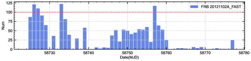
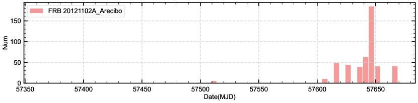
Figure 1: Log of the observations of FRB 20121102A by FAST and Arecibo. The upper panel shows the number of bursts detected by FAST on each day, and the lower panel correspondingly shows the observations by Arecibo. The horizontal dotted line in the upper panel corresponds to an observed rate of 100 bursts in a single day. It can be clearly seen that only on four days, the observed event rate exceeds this number. The bursts of these four days will be used for single-day periodicity searches in Section 5.1.

2.2 FRB 20180916B

FRB 20180916B is also an active repeater. CHIME detected 107 bursts from it over a time span of nearly 5 years. Apertif also detected 54 bursts from the source over a time span of $\sim 260$ days (Pastor-Marazuela et al., 2021). The observational frequency of CHIME is from 400 MHz to 800 MHz, while the observational frequency of Apertif is from 1.22 GHz to 1.52 GHz. FRB 20180916B is reported to have a long-time period of $\sim$ 16.35 days, with an activity window of $\sim 5$ days (CHIME/FRB Collaboration et al., 2020). Recent observations suggested that its active window is both narrower and earlier at higher frequencies (Pastor-Marazuela et al., 2021). FRB 20180916B is associated with a nearby spiral galaxy at a redshift of $z=0.0337$ (Marcote et al., 2020). A brief log of the observations of FRB 20180916B is summarized in Table 1, and the number of bursts observed by CHIME and Apertif on each day is illustrated in Fig. 2.

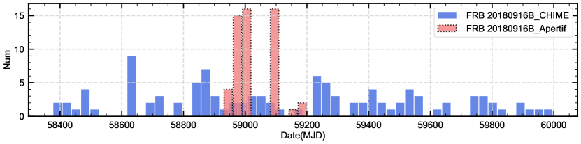
Figure 2: Log of the observations of FRB 20180916B by CHIME and Apertif.

2.3 FRB 20190520B

FRB 20190520B is a special repeater with an very large DM excess, which is therefore believed to occur in an extreme magneto-ionic environment. It was found to be associated with a compact persistent radio source in a dwarf host galaxy at a redshift of $z=0.241$ with a high specific star formation rate (Niu et al., 2022b). FAST detected 79 bursts from FRB 20190520B over a time span of $\sim 488$ days beginning in 2019. The observations are performed in a frequency range of 1.05 GHz–1.45 GHz. A brief log of the observations of FRB 20190520B is summarized in Table 1. The number of bursts observed by FAST on each day is illustrated in Fig. 3.

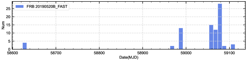
Figure 3: Log of the observations of FRB 20190520B by FAST.

2.4 FRB 20200120E

A total number of 60 bursts were detected from FRB 20200120E by Effelsberg over a time span of $\sim 62$ days (Nimmo et al., 2023). Especially, a burst storm of 53 events occurring in a short period of 40 mins are detected from this source on Jan 14, 2022. The observational frequency is 1.255 GHz–1.505 GHz for Effelsberg. FRB 20200120E is not far from us. Its distance is only 3.6 Mpc. It is associated with a globular cluster in a nearby galaxy (Kirsten et al., 2022). On average, the pulse width of the bursts from FRB 20200120E are much narrower than that of others (by about one order of magnitude). The burst luminosity is also significantly lower. The spectra of its bursts are generally well described by a steep power-law function. Comparing with other repeaters, both the DM and the variation of DM of FRB 20200120E are quite low, which means a relatively clean local magneto-ionic environment (Nimmo et al., 2023). A brief log of the observations of FRB 20200120E is summarized in Table 1. The number of bursts observed by Effelsberg on each day is illustrated in Fig. 4.

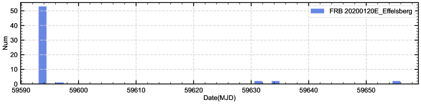
Figure 4: Log of the observations of FRB 20200120E by Effelsberg.

2.5 FRB 20201124A

FRB 20201124A is an extremely active repeater, with nearly $\sim 2000$ bursts being detected. The observations were conducted mainly by FAST and uGMRT. FAST detected 1863 bursts from it over a time span of only $\sim 53$ days beginning in April 2021 (Xu et al., 2022). Note that all these bursts occurred in a total time period of 88 hours, thus leading to a high average event rate of $\sim 21$ bursts per hour. The observational frequency is 1.0 GHz–1.5 GHz. uGMRT also detected 48 FRBs from it on a single day (April 5, 2021), covering a frequency range of 550 MHz–750 MHz (Marthi et al., 2021). The RM of FRB 20201124A varies significantly on a short timescale. A high degree of circular polarization is observed in a good fraction of bursts. FRB 20201124A is associated with a barred spiral galaxy at a redshift of $z=0.098$, located in a region of low stellar density (Xu et al., 2022). A brief log of the observations of FRB 20201124A is summarized in Table 1. The number of bursts observed by FAST and uGMRT on each day is illustrated in Fig. 5.

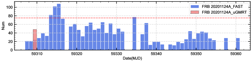
Figure 5: Log of the observations of FRB 20201124A by FAST and uGMRT. The horizontal dotted line corresponds to an observed rate of 75 bursts in a single day. It can be clearly seen that only on four days, the observed event rate exceeds this number. The bursts of these four days will be used for single-day periodicity searches in Section 5.1.

3 Methods

In this study, three different methods are used for periodicity analysis of the above five active repeaters: the phase folding algorithm, the Schuster periodogram, and the Lomb-Scargle periodogram. Among them, the phase folding algorithm is a time-domain method, while the Schuster periodogram and Lomb-Scargle periodogram are frequency-domain methods. Here we describe the three methods briefly.

3.1 The phase folding algorithm

The phase folding algorithm is a traditional but useful and practical method to analyze the time of arrivals of FRBs. Many other analysis methods such as those based on Fourier transforms require additional intensity data. However, the phase folding algorithm only requires a sequence of timing data as the inputs. Considering the diversity of the FRB data sources and the incompleteness and disunity of the data sample itself, the phase folding algorithm is even more credible to some extent.

To begin the analysis, we first assume a trial period ($p$) for the timing data. The time of arrivals of the FRBs are then folded with respect to this assumptive period. Usually, the first data point of the sequence ($t_{0}$) is taken as the zero point. Then the phase of a particular burst that occurs at $t_{i}$ can be calculated as

$$P_{i}=\frac{\big{[}(t_{i}-t_{0})\bmod p\big{]}}{p},$$ (1)

where $\bmod$ means a remainder operation. If $p$ is really the intrinsic period of the timing sequence, then a large number of bursts will concentrate at some particular phase. On the other hand, if $p$ is not the period, then the bursts will randomly distribute at all phases so that no prominent structures will be seen in the phase space. The classic Pearson $\chi^{2}$ test can be used to assess whether $p$ is a potential period or not.

For a particular trial period $p$, when the phases of all the bursts have been determined, we group the bursts into $n$ bins in the phase space. The $\chi^{2}$ value is then calculated as

$$\chi^{2}=\sum_{i=1}^{n}\frac{(O_{i}-E_{i})^{2}}{E_{i}},$$ (2)

where $O_{i}$ is the observed count in the $i$-th bin, and $E_{i}$ is the expected count in each bin for a uniform phase distribution. Here the uniform phase distribution means all the bursts distribute uniformly in the whole phase space. Usually, a large $\chi^{2}$ value indicates that $p$ could potentially be the period of the burst activity, while a small $\chi^{2}$ value means that $p$ is unlikely the intrinsic period. Varying $p$ in all the possible period ranges, we would be able to find the true period if it really exists.

The phase folding method is relatively insensitive to the randomly occurring gaps in the observational data as long as the exposure is reasonably uniform across the phase space. Note that the event rate of FRBs are connected to the detection rate of bursts, i.e. the number of bursts observed by a particular telescope during a unit time period. This factor can be considered in the phase folding procedure by implementing a more precise calculation of $\chi^{2}$, in which $E_{i}$ should be substituted by $T_{i}\cdot\sum O_{i}/\sum T_{i}$, where $T_{i}$ is the exposure time for the $i$th bin (CHIME/FRB Collaboration et al., 2020). For this purpose, we need to know the telescope’s observational time interval associated with each burst. However, in our data sample, such information is not available for all the bursts. So, we simply calculate the $\chi^{2}$ in its original form in this study.

3.2 The Schuster periodogram

The Schuster periodogram, also known as the Schuster spectrum or classical periodogram analysis, is a method widely used to identify periodicity in a timing data set. It was first proposed by Arthur Schuster (Schuster, 1898). The merit of the Schuster periodogram lies in its measurement of the correlation between the time-series data and the sine and cosine functions at different frequencies (i.e. the Fourier series). It calculates the power of each frequency component and identifies the periodic components with the highest normalized power values. This method help revealing the dominant periodic components in the data and their contributions to the overall signal.

The Schuster periodogram relies on the theory of Fourier transform. For the observed time series, the power of Schuster periodogram can be derived by using the formula of discrete Fourier transform:

$$P_{\rm{Schuster}}(\omega) = \frac{1}{N}\left|\sum_{l=1}^{N}g_{l}e^{-i\omega t_{l}}\right|^{2}$$ (3)

$$= \frac{1}{N}\left[\left(\sum_{l=1}^{N}g_{l}\cos(\omega t_{l})\right)^{2}+\left(\sum_{l=1}^{N}g_{l}\sin(\omega t_{l})\right)^{2}\right],$$

where $\omega$ is the angular frequency, $g_{l}$ is the observed signal value of the $l$th data point, $t_{l}$ is the time of the $l$th data point, and $N$ is the total number of data points.

However, the Schuster periodogram has some limitations, such as the spectral leakage and resolution constraints. To overcome these limitations, people have developed more advanced techniques, such as the Lomb-Scargle periodogram described below, which offer improved performance and accuracy in detecting periodicities in a time-series data set.

3.3 The Lomb-Scargle periodogram

Based on the Schuster method, a more effective periodogram was developed by Lomb (1976) and Scargle (1982), which calculate the power as:

$$\begin{split}P_{\rm{Lomb-Scargle}}(\omega)=\frac{1}{2}&\Bigg{\{}\dfrac{\big{[}\sum_{l}g_{l}\cos\omega(t_{l}-\tau)\big{]}^{2}}{\sum_{l}\cos^{2}\omega(t_{l}-\tau)}\\ &+\dfrac{\big{[}\sum_{l}g_{l}\sin\omega(t_{l}-\tau)\big{]}^{2}}{\sum_{l}\sin^{2}\omega(t_{l}-\tau)}\Bigg{\}},\end{split}$$ (4)

where $\omega$ is the angular frequency, $g_{l}$ is the observed signal value of the $l$th data point, $t_{l}$ is the time of the $l$th data point, and $\tau$ is specified for each $\omega$ to ensure the time-shift invariance:

$$\tau=\frac{1}{2\omega}\tan^{-1}\Bigg{(}\frac{\sum_{l}\sin 2\omega t_{l}}{\sum_{l}\cos 2\omega t_{l}}\Bigg{)}.$$ (5)

where $l$ ranges from 1 to $N$ in the summation. $N$ is the total number of data points.

The Lomb-Scargle periodogram is an improved method for periodogram analysis that has several notable advantages over the Schuster periodogram. Especially, it is more effective in analyzing time-series data that have non-uniformly distributed sampling intervals. In reality, data collection may be affected by complicated factors such as observation conditions and instrument limitations, resulting in unevenly spaced intervals. The Lomb-Scargle method is more suitable in these cases. The main limitation of the Lomb-Scargle periodogram is the much higher computational complexity being involved.

3.4 Segmented period searches

In our study, we generally need to search for a short timescale period (0.001 s to 1000 s) by using observational data spanning a long term (months or even years). Note that the trial period varies in a wide range, which essentially covers six orders of magnitude. Under this circumstance, the procedure is very difficult and too much calculations are needed no matter whether we use the phase folding algorithm, the Schuster periodogram, or the Lomb-Scargle periodogram. The reason is that a huge amount of data are involved in the analysis, which poses a challenge for the computer’s memory capacity and processing speed.

To overcome the difficulty, we divide the target period range into six segments, i.e., 0.001 s–0.01 s, 0.01 s–0.1 s, 0.1 s–1 s, 1 s–10 s, 10 s–100 s, and 100 s–1000 s. An appropriate period step are applied in each segment. In this way, we can thoroughly examine possible periodicity in the whole range of 1 ms–1000 s.

4 Global period searches for five FRBs

In this section, we present our results of period searching for the five repeating FRBs. All the three methods described above are applied to each repeater. In our study, we mainly concentrate on short-time periodicity, with the period ranging in 0.001 s–1000 s. As mentioned above, to improve the efficiency, the whole period range is divided into six segments, i.e. 0.001 s–0.01 s, 0.01 s–0.1 s, … , 100 s–1000 s. The period step is taken as 5 $\mathrm{\mu s}$, 50 $\mathrm{\mu s}$, … , 0.5 s in each segment, respectively. Such a strategy significantly reduces the computing burden. It can meet the requirement of the expected accuracy as well. Here in this section, for each repeating source, the arrival times of all the detected bursts are used in the searching process.

4.1 FRB 20121102A

The arrival times of all the bursts from FRB 20121102A, obtained by FAST and Arecibo, are used to search for potential short-time periodicity. Here, the arrival time corresponds to the peak of each burst, calibrated to the barycenter of the solar system. For the FAST data set, the arrival times are de-dispersed and normalized to 1.5 GHz. The timing accuracy of this FAST FRB sample (estimated from the last digit of the recorded arrival time) is $\sim 10^{-9}$ d (86.4 $\mathrm{\mu s}$), which means it is accurate enough to reveal any potential periodicity with a period larger than $\sim 1$ ms. Correspondingly, the arrival times of Arecibo data set are de-dispersed and normalized to the infinite frequency. The timing accuracy is also $10^{-9}$ d (86.4 $\mathrm{\mu s}$).

We have used all the three methods mentioned above to analyze the periodicity in FRB 20121102A. For the the Schuster and Lomb-Scargle methods, we use the fluence of each burst as a necessary input for the intensity. The data sets of FAST and Arecibo are analyzed separately to avoid any possible systematic difference between them. The results are shown in Fig. 6. For the phase folding method and the Schuster periodogram, a horizontal dotted line is plot to mark the coincidence level of $10^{-5}$. Correspondingly, for the Lomb-Scargle periodogram, a horizontal dotted line showing a coincidence level of $0.001$ is plot. From these plots, we can clearly see that no periodicity exceeding these confidence levels is found in the whole range of 0.001–1000 s for FRB 20121102A. In each segment, we have also examined by hand the phase-folded histogram at the position that corresponds to the highest $\chi^{2}$ value, but found that no marked features appear in the histogram.

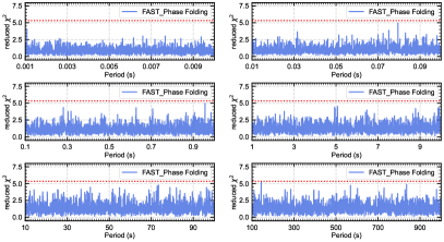
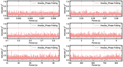
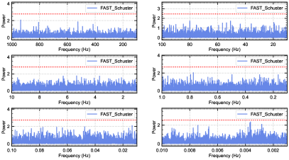
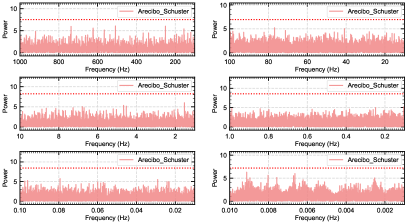
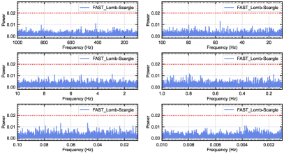
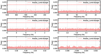
Figure 6: The results of periodicity analysis for FRB 20121102A. The left two columns are the results by using FAST data, and the right two columns are the results by using Arecibo data. Three methods are applied for each dataset, i.e., the phase folding method, the Schuster periodogram, and the Lomb-Scargle periodogram. The results are shown in the panels from top to bottom, respectively. In the panels corresponding to the phase folding method and Schuster periodogram, the horizontal dotted lines represent a coincidence level of $<10^{-5}$. In the panels corresponding to the Lomb-Scargle periodogram, the horizontal dotted lines represent a coincidence level of $<0.001$. No clear evidence of periodicity is found in these plots.

4.2 FRB 20180916B

The arrival times of all the bursts from FRB 20180916B, obtained by CHIME and Apertif, are used to search for potential short-time periodicity. Again, the arrival time corresponds to the peak of each burst, calibrated to the barycenter of the solar system. For the CHIME data set, the arrival times are de-dispersed and normalized to the infinite frequency. The timing accuracy of this CHIME FRB sample (estimated from the last digit of the recorded arrival time is $\sim 1\mathrm{\mu s}$), which is high enough. The arrival times of Apertif data set are de-dispersed and normalized to a frequency of 1.4 GHz. However, note that the timing accuracy of the Apertif data set is $10^{-8}$ d (864 $\mathrm{\mu s}$), which means it is not accurate enough to reveal any potential periodicity with a period less than $\sim 10$ ms.

We have also used all the three methods to analyze the periodicity in FRB 20180916B. For the Schuster and Lomb-Scargle methods, we use the Apertif fluence as the necessary input for the intensity. However, since the CHIME data set do not contain fluences, we use the signal-to-noise ratio as the input for the intensity. The data sets of CHIME and Apertif are analyzed separately to avoid any possible systematic difference between them. The results are shown in Fig. 7. For the phase folding method and the Schuster periodogram, a horizontal dotted line is plot to mark the coincidence level of $10^{-5}$. Correspondingly, for the Lomb-Scargle periodogram, a horizontal dotted line showing a coincidence level of $0.001$ is plot. From these plots, we can see that no periodicity exceeding these confidence levels is found in the whole range of 0.001–1000 s for FRB 20180916B. In each segment, we again have examined the phase-folded histogram at the position that corresponds to the highest $\chi^{2}$ value, but found that no marked features appear in the histogram.

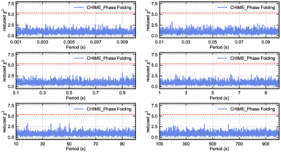
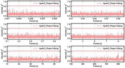
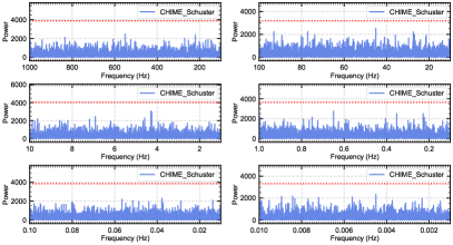
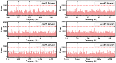
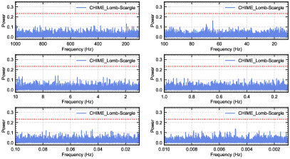
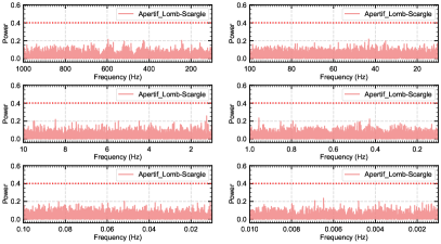
Figure 7: The results of periodicity analysis for FRB 20180916B. The left two columns are the results by using CHIME data, and the right two columns are the results by using Apertif data. Three methods are applied for each dataset, i.e., the phase folding method, the Schuster periodogram, and the Lomb-Scargle periodogram. The results are shown in the panels from top to bottom, respectively. In the panels corresponding to the phase folding method and Schuster periodogram, the horizontal dotted lines represent a coincidence level of $<10^{-5}$. In the panels corresponding to the Lomb-Scargle periodogram, the horizontal dotted lines represent a coincidence level of $<0.001$. No clear evidence of periodicity is found in these plots.

4.3 FRB 20190520B

The arrival times of all the bursts from FRB 20190520B, obtained by FAST, are used to search for potential short-time periodicity. The arrival time corresponds to the peak of each burst, calibrated to the barycenter of the solar system. All the arrival times are de-dispersed and normalized to 1.5 GHz. The timing accuracy of this FAST FRB sample (estimated from the last digit of the recorded arrival time) is $10^{-9}$ d (86.4 $\mathrm{\mu s}$), which is high enough to reveal any potential periodicity with a period larger than $\sim 1$ ms.

All the three methods described in the previous section are used to analyze the periodicity in FRB 20190520B. For the Schuster and Lomb-Scargle methods, we still use the fluence as the necessary input for the intensity. The results are shown in Fig. LABEL:Fig8. For the phase folding method and the Schuster periodogram, a horizontal dotted line is plot to mark the coincidence level of $10^{-5}$. Correspondingly, for the Lomb-Scargle periodogram, a horizontal dotted line showing a coincidence level of $0.001$ is plot. From these plots, we can see that no periodicity exceeding these confidence levels is found in the whole range of 0.001–1000 s for FRB 20190520B. In each segment, we have examined the phase-folded histogram at the position with the highest $\chi^{2}$ value, but found that no marked features appear in the histogram.

4.4 FRB 20200120E

The arrival times of all the bursts from FRB 20200120E, obtained by Effelsberg, are used to search for potential short-time periodicity. The arrival time corresponds to the peak of each burst, calibrated to the barycenter of the solar system. All the arrival times are de-dispersed and normalized to the infinite frequency. The timing accuracy of this Effelsberg FRB sample (estimated from the last digit of the recorded arrival time) is $10^{-8}$ d (864 $\mathrm{\mu s}$), which means it is not accurate enough to reveal the potential periodicity with a period less than $\sim 10$ ms.

All the three methods described in the previous section are used to analyze the periodicity in FRB 20200120E. For the Schuster and Lomb-Scargle methods, we still use the fluence as the necessary input for the intensity. The results are shown in Fig. LABEL:Fig9. For the phase folding method and the Schuster periodogram, a horizontal dotted line is plot to mark the coincidence level of $10^{-5}$. Correspondingly, for the Lomb-Scargle periodogram, a horizontal dotted line showing a coincidence level of $0.001$ is plot. From these plots, we can see that no periodicity exceeding these confidence levels is found in the whole range of 0.001–1000 s for FRB 20200120E. In each segment, we have examined the phase-folded histogram at the position with the highest $\chi^{2}$ value, but found that no marked features appear in the histogram. But note that the possible existence of a periodicity in 1 ms–10 ms still could be completely excluded yet, due to the limited timing accuracy.

4.5 FRB 20201124A

The arrival times of all the bursts from FRB 20201124A, obtained by FAST and uGMRT, are used to search for potential short-time periodicity. The arrival time corresponds to the peak of each burst, calibrated to the barycenter of the solar system. For the FAST data set, the arrival times are de-dispersed and normalized to 1.5 GHz. The timing accuracy of this FAST FRB sample (estimated from the last digit of the recorded arrival time) is $10^{-8}$ d (864 $\mathrm{\mu s}$), which means it is not accurate enough to reveal the potential periodicity with a period less than $\sim 10$ ms. The arrival times of uGMRT data set are de-dispersed and normalized to a frequency of 550 MHz. Again, the timing accuracy of the uGMRT data set is $10^{-8}$ d (864 $\mathrm{\mu s}$), which is not accurate enough to reveal the potential periodicity with a period less than $\sim 10$ ms.

We have used all the three methods described in the previous section to analyze the periodicity in FRB 20201124A. For the the Schuster and Lomb-Scargle methods, we use the fluence of each burst as a necessary input for the intensity. The data sets of FAST and uGMRT are analyzed separately to avoid any possible systematic difference between them. The results are shown in Fig. 10. For the phase folding method and the Schuster periodogram, a horizontal dotted line is plot to mark the coincidence level of $10^{-5}$. Correspondingly, for the Lomb-Scargle periodogram, a horizontal dotted line showing a coincidence level of $0.001$ is plot. Note that in the upper-left panel of Fig. 10 which shows the FAST result in the 0.001–0.01 s range, several extremely high peaks could be observed. However, all these peaks correspond to a too short period that is less than 10 ms. They are actually fake signals due to the limitation of the timing accuracy. The inset in the panel shows the folding result at one of the peaks. Still, from Fig. 10, we can conclude that no periodicity exceeding the expected confidence levels is found in the whole range of 0.005–1000 s for FRB 20201124A. In other segments, we have also examined the phase-folded histogram at the position with the highest $\chi^{2}$ value, but found that no marked features appear in the histogram.

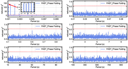
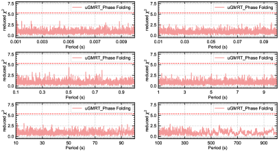
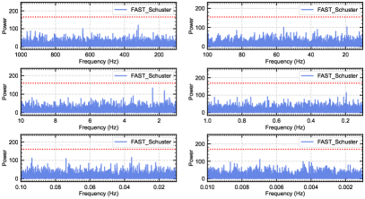
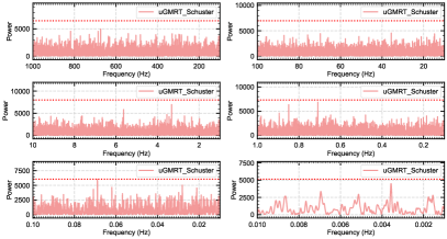
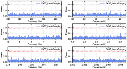
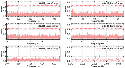
Figure 10: The results of periodicity analysis for FRB 20201124A. The left two columns are the results by using FAST data, and the right two columns are the results by using uGMRT data. Three methods are applied for each dataset, i.e., the phase folding method, the Schuster periodogram, and the Lomb-Scargle periodogram. The results are shown in the panels from top to bottom, respectively. In the panels corresponding to the phase folding method and Schuster periodogram, the horizontal dotted lines represent a coincidence level of $<10^{-5}$. In the panels corresponding to the Lomb-Scargle periodogram, the horizontal ddotted lines represent a coincidence level of $<0.001$. No clear evidence of periodicity is found in these plots. Note that in the upper-left panel that shows the FAST result in the 0.001–0.01 s range, the peak structures at $<10$ ms are fake signals due to the limited timing accuracy. The inset in the panel shows the folding result at one of the peaks.

To summarize, we have carefully examined the five active repeating FRB sources. All the three methods widely used for periodicity analysis are applied on them. For three of them (FRBs 20121102A, 20180916B, 20190520B), no evidence is found supporting the existence of any periodicity in the whole range of 0.001 s–1000 s. For FRBs 20200120E and 20201124A, also a negative result is obtained for the wide range of 0.01 s–1000 s. However, no firm conclusion could be drawn for the period range of 0.001 s–0.01 s yet, due to the limited timing accuracy of currently available observations.

5 More in-depth period searches for FRBs 20121102A and 20201124A

Here, we concentrate on the two most active repeaters, FRBs 20121102A and 20201124A. These two FRBs exhibit both a high burst rate and a high total number of bursts being detected. During two observation campaigns conducted by FAST, an astonishing number of 1652 bursts were detected from FRB 20121102A, and also 1863 bursts were detected from FRB 20201124A. Using these large samples, we can conduct more thorough searches for short timescale periodicity in these two FRBs.

5.1 Single-day period searches

In our study, we have tried to select those days on which a large number of bursts were detected by FAST during the observation of a single day. We use these bursts to search for potential period exists in each of those days. Then we combine the results of those days jointly by calculating the correlation function among them. In this way, we would be able to find any common periods existed in the bursts of those days. The advantage of performing such a single-day period search is that it can effective eliminate possible systematic timing errors on different days. For example, if 100 bursts were detected by FAST in a two-hour monitoring, then the time intervals between every two successive FRBs will be recorded with an extremely high accuracy. The relative arrival times of these 100 bursts will not be subject to any serious systematic errors when they are calibrated to the barycenter of the solar system, thus they can effectively reserve their intrinsic period information. Additionally, by using the cross-correlation method, we can also effectively improve the reliability of the period search.

As shown in Fig. 1, a total number of 1652 bursts are detected from FRB 20121102A by FAST. We see that there are four days (MJDs 58725, 58726, 58732, and 58756) on which the number of detected single-day bursts is larger than 100. Note that the number of single-day bursts here is even larger than the number of all bursts detected from other active sources, such as FRBs 20180916B, 20190520B, and 20200120E (see Table 1). We have selected these four days and analyzed their periodicity on each day. All the three methods, i.e. the phase folding, Schuster and Lomb-Scargle periodogram, are applied in our analysis. The results of these four days are then combined to search for any potential common periods among them. The results are shown in Fig. 11. Note that for clarity, Fig. 11 only includes the results of the phase folding analysis. The figures corresponding to the Schuster and Lomb-Scargle periodogram methods are presented in the Appendix. Here, the whole period range of 0.001 s–1000 s is still divided into 6 segments, i.e. 0.001 s–0.01 s, 0.01 s–0.1 s, 0.1 s–1 s, 1 s–10 s, 10 s–100 s, and 100 s–1000 s. In each segment, the bursts detected by FAST on each of the four days are first analyzed separately. The results are then cross-correlated to search for their possible common periods. In our study, we have selected the best candidate period in each segment and plot the distribution of the bursts in the phase space folded according to the candidate period. Generally, we could clearly see that the structures are not prominent in all the histograms. Our in-depth search thus still fails to find any short timescale periodicity in FRB 20121102A.

Similarly, as shown in Fig. 5, a total number of 1863 bursts are detected from FRB 20201124A by FAST. We have chosen four days on which the most bursts are detected, i.e. MJDs 59313, 59314, 59315, and 59334. On each day, the number of detected bursts is larger than 70. We have analyzed their periodicity by using the phase folding method. The results of these four days are then combined to search for any potential common periods among them. The results of the phase folding method are shown in Fig. 12, and those corresponding to the Schuster and Lomb-Scargle periodogram methods are also presented in the Appendix. Similar to that in Fig. 11, here the whole period range of 0.001 s–1000 s is still divided into 6 segments. In each segment, the bursts detected by FAST on each of the four days are first analyzed separately. The results are then cross-correlated to search for their possible common periods. Again, we have selected the best candidate period in each segment and plot the corresponding distribution of the bursts in the phase space. Note that for FRB 20201124A, since the timing accuracy of FAST observations is $864\mathrm{\mu s}$, the periodicity with a period less than $\sim 10$ ms could be fake signals (also see Section 4.5). Apart from the uncertain range of 1 ms–10 ms, we see that the structures are not prominent in the histograms in all other segments. FRB 20201124A thus does not show any periodicity among the 10 ms–1000 s range in this in-depth search.

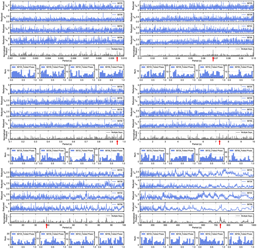
Figure 11: In-depth period search results of FRB 20121102A by using the phase folding method. Again, the whole period range of 0.001 s–1000 s is divided into 6 segments, i.e. 0.001 s–0.01 s, 0.01 s–0.1 s, 0.1 s–1 s, 1 s–10 s, 10 s–100 s, and 100 s–1000 s. In each segment, the bursts detected by FAST on four days are analyzed (MJDs 58725, 58726, 58732, and 58756, marked in each panel correspondingly): the first four panels show the phase folding results for each of the four days, then the fifth panel shows their cross-correlation function, i.e. an normalized product of the above four panels. An arrow is marked at the position (the best candidate period) that has the highest product. The histograms just below the correlation function panel show the distribution of the bursts in the phase space folded according to the best candidate period as marked by the arrow, for the four days.

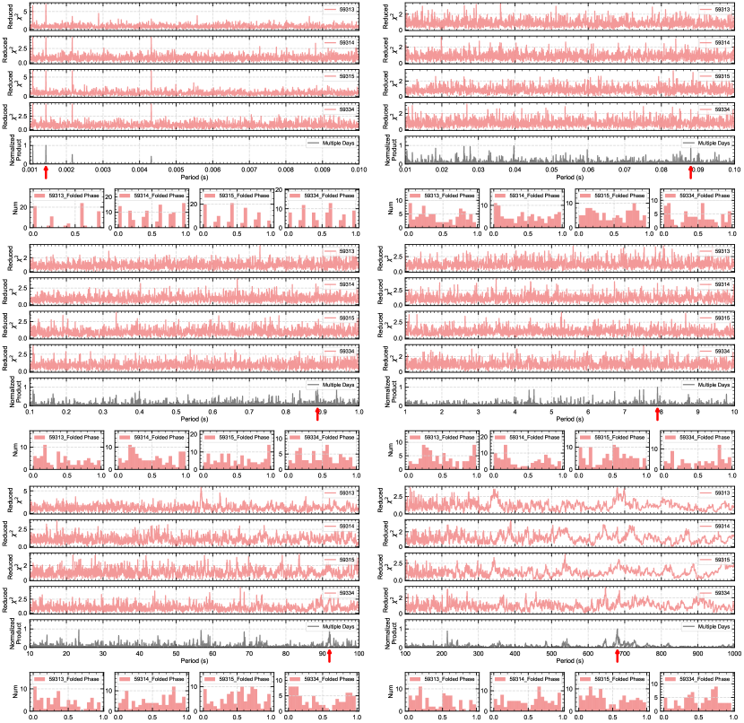
Figure 12: In-depth period search results of FRB 20201124A by using the phase folding method. Similar to Fig. 11, the whole period range of 0.001 s–1000 s is divided into 6 segments, i.e. 0.001 s–0.01 s, 0.01 s–0.1 s, 0.1 s–1 s, 1 s–10 s, 10 s–100 s, and 100 s–1000 s. In each segment, the bursts detected by FAST on four days are analyzed (MJDs 59313, 59314, 59315, and 59334, marked in each panel correspondingly): the first four panels show the phase folding results for each of the four days, then the sixth panel shows their cross-correlation function, i.e. an normalized product of the above four panels. An arrow is marked at the position (the best candidate period) that has the highest product. The histograms just below the correlation function panel show the distribution of the bursts in the phase space folded according to the best candidate period as marked by the arrow, for the four days. Note that since the timing accuracy of FAST observations is $864\mathrm{\mu s}$ for FRB 20201124A, the structures of the histograms in the first segment (0.001 s–0.01 s) with a period less than $\sim 10$ ms should be fake signals, which can be clearly seen in the corresponding histograms.

5.2 Period search based on classification

FRBs are highly variable. Their properties vary from event to event. They have different pulse widths, peak flux, fluence and pulse profiles, and the emission is in different frequency ranges. The differences may reflect the different physical conditions of the central engine. Theoretically, even for the same repeater, the bursts might be triggered by different mechanisms and could be emitted at various regions. Therefore, it is possible that some subclasses of FRBs may show a periodical behavior. In this subsection, we explore the periodicity of FRBs based on their properties. In earlier researches of repeating FRBs, the small sample size severely limits the robustness of previous attempts at period searching on subclasses of bursts. However, thanks to the large samples of FRB 20121102A and FRB 20201124A obtained by FAST, it is possible for us to group the sample to subsets and examine their nature in great detail.

As a first step, we have tried to use some simple parameters such as the pulse width, peak flux or fluence as the weighting factor of each burst, and repeated the previous search processes. Unfortunately, no clear evidence pointing toward any periodicity is found.

We then consider the brightness temperature as the criteria. Recent studies by Xiao & Dai (2022b); Xiao & Dai (2022a) suggest that FRBs can be divided into two subsets according to their brightness temperatures: typical bursts and bright bursts. Here we present our results of period search for these two subclasses of FRBs.

The brightness temperature of an FRB is defined by equaling the observed power to the luminosity of a blackbody, which gives:

$$T_{\mathrm{B}}=F_{\nu}d_{\mathrm{A}}^{2}/2\pi k(\nu\cdot W)^{2},$$ (6)

where $F_{\nu}$ is the flux density, $\nu$ is the emission frequency and $W$ is the pulse width. Note that $d_{\mathrm{A}}$ here is the angular diameter distance, which is different for different repeaters. In this study, a flat $\Lambda$-CDM cosmology with $H_{0}=67.4$ km s^-1 Mpc^-1 and $\Omega_{\rm m}=0.315$ is adopted (Planck Collaboration et al., 2020). For FRB 20121102A at a redshift of $z=0.19273$ (Tendulkar et al., 2017), we get the distance as $d_{\mathrm{A}}$ = 0.682 Gpc. For FRB 20201124A at $z=0.09795$ (Xu et al., 2022), we have $d_{\mathrm{A}}$ = 0.386 Gpc. Fig. 13 shows the distribution of FRBs on the $W$ - $F_{\nu}$ plane for both FRB 20121102A and FRB 20201124A. In our calculations below, we take $T_{B}=10^{33}$ K as the criterion between typical bursts and bright bursts for both FRB 20121102A and FRB 20201124A. This criterion is consistent with that suggested by Xiao & Dai (2022b).

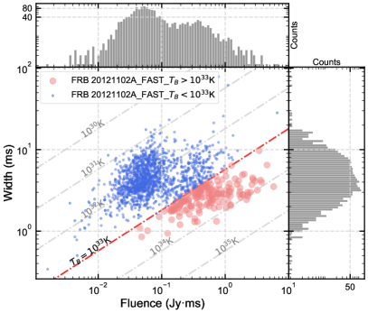
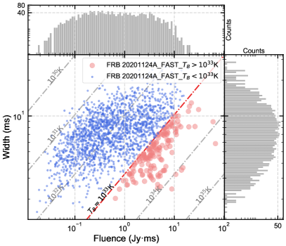
Figure 13: The distribution of FRBs on the $W$ - $F_{\nu}$ plane. The left panel shows the case of FRB 20121102A, and the right panel shows the case of FRB 20201124A. The oblique dashed lines in each panel correspond to different brightness temperatures. $T_{B}=10^{33}$ K is taken as the criterion between typical bursts and bright bursts for both FRB 20121102A and FRB 20201124A.

We have performed periodicity analysis on the two subsets of FRBs, i.e. typical bursts and bright bursts, separately. Fig. 14 presents our results for FRB 20121102A by using the phase folding method. We see that no periodicity is found neither in typical bursts nor in bright bursts. We have also done the analysis by using the Schuster method and the Lomb-Scargle periodogram method. The results are shown in the Appendix. Still, no evidence pointing toward the existence of any periodicity is found for FRB 20121102A.

Similarly, Fig. 15 presents our results based on classification for FRB 20201124A. Again, the analysis is done by using the phase folding method. We see that no periodicity is found neither in typical bursts nor in bright bursts. We have also done the analysis by using the Schuster method and the Lomb-Scargle periodogram method. The results are shown in the Appendix. Still, no periodicity is found for FRB 20201124A.

Note that in Fig. 15, some prominent peak structures can be found in the two panels showing the results of the 0.001–0.01 s segment. Their corresponding periods are all less than $10$ ms and are fake signals due to timing errors. For FRB 20201124A, the timing accuracy of the FAST data set is $10^{-8}$ d (864 $\mathrm{\mu s}$), which means it is not accurate enough to reveal any potential periodicity with a period less than $\sim 10$ ms.

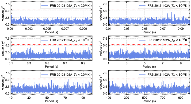
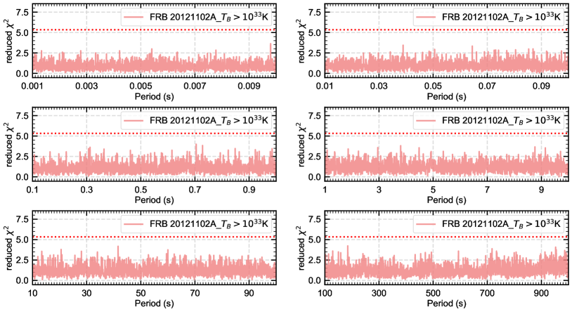
Figure 14: Periodicity analysis for FRB 20121102A based on classification according to the brightness temperature. The phase folding method is applied in the analysis. The upper six panels correspond to typical bursts with $T_{B}<10^{33}$ K, and the lower six panels correspond to the bright subset of bursts with $T_{B}>10^{33}$ K. For each subset, the whole period range of 0.001 s–1000 s is divided into 6 segments, i.e. 0.001 s–0.01 s, 0.01 s–0.1 s, 0.1 s–1 s, 1 s–10 s, 10 s–100 s, and 100 s–1000 s. The horizontal dotted line in each panel represents a coincidence level of $<10^{-5}$. No clear evidence of periodicity is found in these plots.

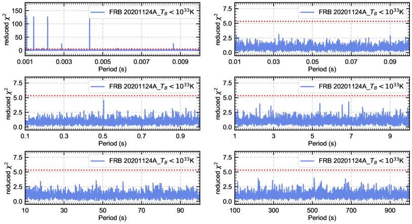
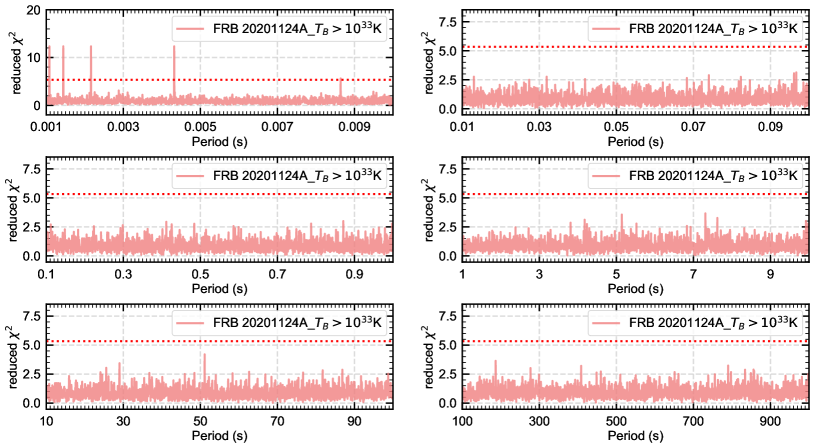
Figure 15: Periodicity analysis for FRB 20201124A based on classification according to the brightness temperature. The phase folding method is applied in the analysis. The upper six panels correspond to typical bursts with $T_{B}<10^{33}$ K, and the lower six panels correspond to the bright subset of bursts with $T_{B}>10^{33}$ K. For each subset, the whole period range of 0.001 s–1000 s is divided into 6 segments, i.e. 0.001 s–0.01 s, 0.01 s–0.1 s, 0.1 s–1 s, 1 s–10 s, 10 s–100 s, and 100 s–1000 s. The horizontal dotted line in each panel represents a coincidence level of $<10^{-5}$. No clear evidence of periodicity is found in these plots. Note that in the two panels that show the results in the 0.001 s–0.01 s range, the peak structures at $<10$ ms are fake signals due to the limitation of the timing accuracy.

6 Conclusions and discussion

Whether short timescale periodicity exists or not in the activities of repeating FRBs is an intriguing issue. In this study, we perform a thorough search for periodicity in the range of 0.001 s–1000 s on the five most active repeaters, i.e. FRBs 20121102A, 20180916B, 20190520B, 20200120E, and 20201124A. Observational data obtained by various telescopes, including CHIME, FAST, Apertif, uGMRT, and Effelsberg are collected and used in the analysis. Three period searching methods are adopted in the process, which include the phase folding algorithm, Schuster periodogram, and Lomb-Scargle periodogram. For the two most active repeating sources, FRBs 20121102A and 20201124A (Li et al., 2018), more in-depth period searches are conducted. We have selected those days on which a large number of bursts were detected and conducted period search based on these single-day events. We have also tried to analyze the data by using the pulse width, peak flux or the fluence as a weight for each burst. Periodicity analysis is also conducted separately for different sub-classes of bursts featured by the brightness temperature. In all the attempts, no evidence pointing to any clear short timescale periodicity is found.

The recurrence of FRBs from a particular source strongly indicates that the bursts are non-catastrophic events. The association of FRB 20200428 with SGR J1935+2154 firmly establishes the connection between magnetars and at least some FRBs (Li et al., 2021a; Mereghetti et al., 2020). As a result, it is naturally expected that periodicity connected with the spinning of magnetars should exist in the activities of repeating FRBs. The properties of FRBs, such as the pulse width, peak flux, fluence, and the brightness temperature, may depend on the detailed trigger mechanism and the position of radiation. However, our study shows that there are no periodical signals in the detected bursts even when the effects of pulse width, peak flux, fluence, and the brightness temperature are considered. Such a null result could provide useful constraints on the theoretical models of repeating FRBs. It may indicate that the radiation is emitted in a region that is relatively far away from the magnetar, at least outside the light cylinder, where the radiation zone does not co-rotate with the magnetar. Another possibility is that the burst activities are not restricted to a particular region of the magnetar. Instead, they could be triggered at different positions on the surface or in the magnetosphere of the compact star. It could also be possible that some external mechanisms such as the collision of asteroids trigger these repeating bursts (Geng & Huang, 2015).

It deserves mentioning that the possible existence of a period less than $\sim 10$ ms still cannot be completely excluded for FRBs 20200120E and 20201124A yet. The observational data of these two repeating sources were obtained by Effelsberg, FAST and uGMRT, but the timing accuracy of the data are $864\mathrm{\mu s}$ during their observations on these repeaters. It is impossible to reveal any periodicity with a period less than $\sim 10$ ms based on the data sets. More accurate observations should be carried out to further examine this issue in the future.

Data Availability

The original data of FRB 20121102A analyzed in the this work are available from Li et al. (2021b) (10.1038/s41586-021-03878-5) and Hewitt et al. (2022) (10.1093/mnras/stac1960). The original data of FRB 20180916B analyzed in the this work are available from CHIME/FRB Public Database (https://www.chime-frb.ca/) and Pastor-Marazuela et al. (2021) (10.1038/s41586-021-03724-8). The original data of FRB 20190520B analyzed in the this work are available from Niu et al. (2022b) (10.1038/s41586-022-04755-5). The original data of FRB 20200120E analyzed in the this work are available from Nimmo et al. (2023) (10.1093/mnras/stad269). The original data of FRB 20201124A analyzed in the this work are available from Xu et al. (2022) (10.1038/s41586-022-05071-8) and Marthi et al. (2021) (10.1093/mnras/stab3067).

Appendix A Additional figures showing the in-depth searching results

In our study, we have carried out detailed periodicity analysis on the five most active repeating FRBs by using three methods, i.e. the phase folding algorithm, the Schuster periodogram, and the Lomb-Scargle periodogram. Major results have been illustrated in the main text. Here in this appendix, we present some additional figures that are not shown in the previous sections. Note that no periodicity is revealed in all the plots below.

Figure 16 illustrates our in-depth analysis on the FAST data of FRB 20121102A based on single-day searches. The observations on four days (MJDs 58725, 58726, 58732, and 58756) are used and the Schuster periodogram method is applied. In Figure 17, the same data are analyzed but the Lomb-Scargle periodogram method is adopted.

Figure 18 illustrates our in-depth analysis on the FAST data of FRB 20201124A based on single-day searches. The observations on four days (MJDs 59313, 59314, 59315, and 59334) are used and the Schuster periodogram method is applied. In Figure 19, the same data are analyzed but the Lomb-Scargle periodogram method is adopted.

Figure 20 illustrates the periodicity analysis results for FRB 20121102A based on classification according to the brightness temperature. The Schuster periodogram method is applied in the analysis. In Figure 21, the same data are analyzed but the Lomb-Scargle periodogram method is adopted.

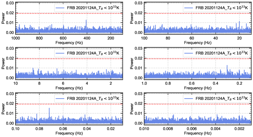
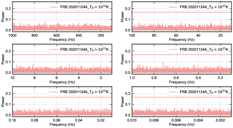
Figure 23: Periodicity analysis for FRB 20201124A based on classification according to the brightness temperature. The Lomb-Scargle periodogram method is applied in the analysis. The upper six panels correspond to typical bursts with $T_{B}<10^{33}$ K, and the lower six panels correspond to the bright subset of bursts with $T_{B}>10^{33}$ K. For each subset, the whole period range of 0.001 s–1000 s is divided into 6 segments, i.e. 0.001 s–0.01 s, 0.01 s–0.1 s, 0.1 s–1 s, 1 s–10 s, 10 s–100 s, and 100 s–1000 s. The horizontal dotted line in each panel represents a coincidence level of $<0.001$. No clear evidence of periodicity is found in these plots.

Figure 22 illustrates the periodicity analysis results for FRB 20201124A based on classification according to the brightness temperature. The Schuster periodogram method is applied in the analysis. In Figure 23, the same data are analyzed but the Lomb-Scargle periodogram method is adopted.

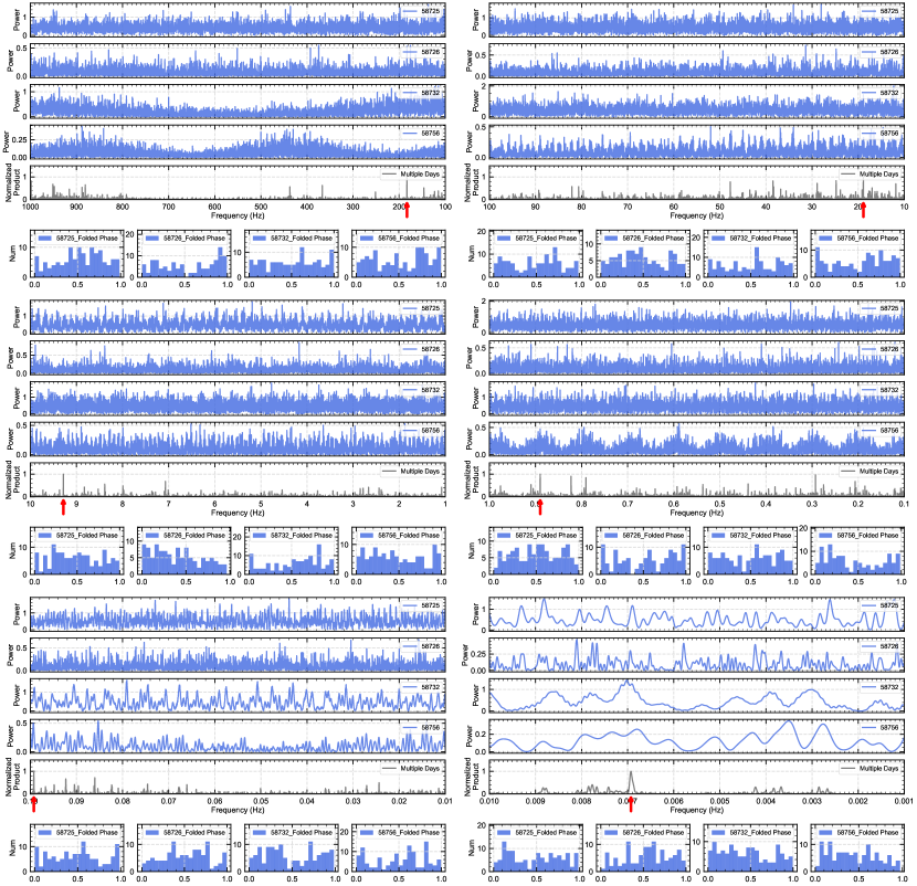
Figure 16: In-depth period search results of FRB 20121102A by using the Schuster periodogram method. The whole period range of 0.001 s–1000 s is divided into 6 segments, i.e. 0.001 s–0.01 s, 0.01 s–0.1 s, 0.1 s–1 s, 1 s–10 s, 10 s–100 s, and 100 s–1000 s. In each segment, the bursts detected by FAST on four days are analyzed (MJDs 58725, 58726, 58732, and 58756, marked in each panel correspondingly): the first four panels show the phase folding results for each of the four days, then the fifth panel shows their cross-correlation function, i.e. an normalized product of the above four panels. An arrow is marked at the position (the best candidate period) that has the highest product. The histograms just below the correlation function panel show the distribution of the bursts in the phase space folded according to the best candidate period as marked by the arrow, for the four days.

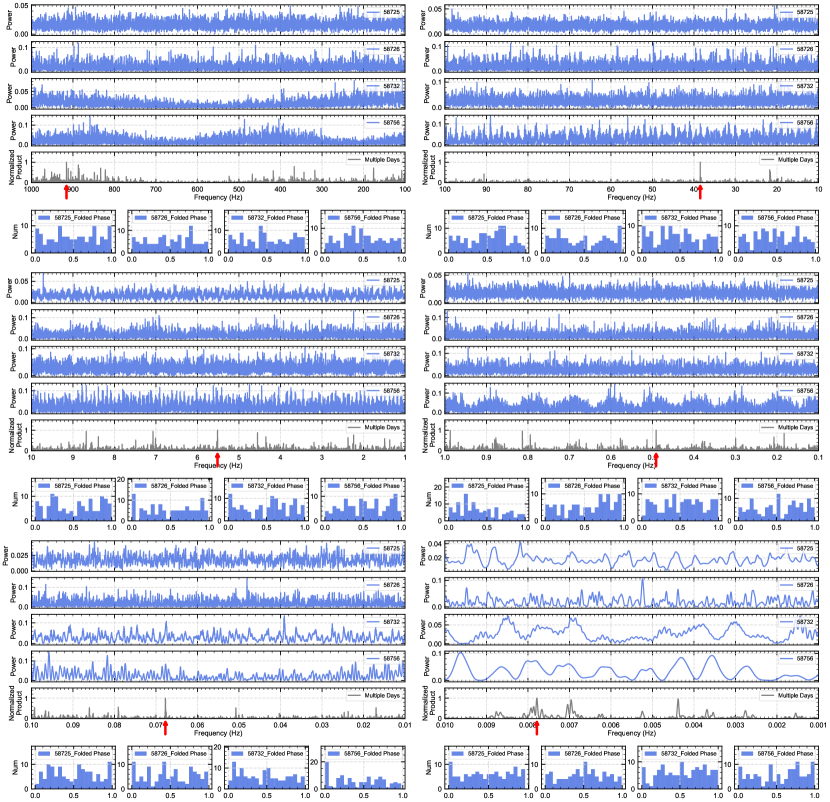
Figure 17: In-depth period search results of FRB 20121102A by using the Lomb-Scargle periodogram method. The whole period range of 0.001 s–1000 s is divided into 6 segments, i.e. 0.001 s–0.01 s, 0.01 s–0.1 s, 0.1 s–1 s, 1 s–10 s, 10 s–100 s, and 100 s–1000 s. In each segment, the bursts detected by FAST on four days are analyzed (MJDs 58725, 58726, 58732, and 58756, marked in each panel correspondingly): the first four panels show the phase folding results for each of the four days, then the fifth panel shows their cross-correlation function, i.e. an normalized product of the above four panels. An arrow is marked at the position (the best candidate period) that has the highest product. The histograms just below the correlation function panel show the distribution of the bursts in the phase space folded according to the best candidate period as marked by the arrow, for the four days.

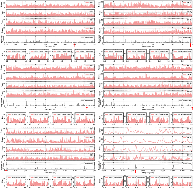
Figure 18: In-depth period search results of FRB 20201124A by using the Schuster periodogram method. The whole period range of 0.001 s–1000 s is divided into 6 segments, i.e. 0.001 s–0.01 s, 0.01 s–0.1 s, 0.1 s–1 s, 1 s–10 s, 10 s–100 s, and 100 s–1000 s. In each segment, the bursts detected by FAST on four days are analyzed (MJDs 59313, 59314, 59315, and 59334, marked in each panel correspondingly): the first four panels show the phase folding results for each of the four days, then the fifth panel shows their cross-correlation function, i.e. an normalized product of the above four panels. An arrow is marked at the position (the best candidate period) that has the highest product. The histograms just below the correlation function panel show the distribution of the bursts in the phase space folded according to the best candidate period as marked by the arrow, for the four days.

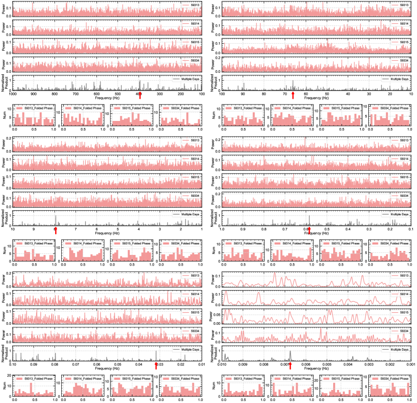
Figure 19: In-depth period search results of FRB 20201124A by using the Lomb-Scargle periodogram method. The whole period range of 0.001 s–1000 s is divided into 6 segments, i.e. 0.001 s–0.01 s, 0.01 s–0.1 s, 0.1 s–1 s, 1 s–10 s, 10 s–100 s, and 100 s–1000 s. In each segment, the bursts detected by FAST on four days are analyzed (MJDs 59313, 59314, 59315, and 59334, marked in each panel correspondingly): the first four panels show the phase folding results for each of the four days, then the fifth panel shows their cross-correlation function, i.e. an normalized product of the above four panels. An arrow is marked at the position (the best candidate period) that has the highest product. The histograms just below the correlation function panel show the distribution of the bursts in the phase space folded according to the best candidate period as marked by the arrow, for the four days.

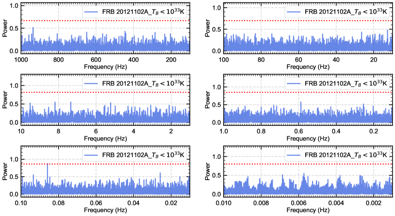
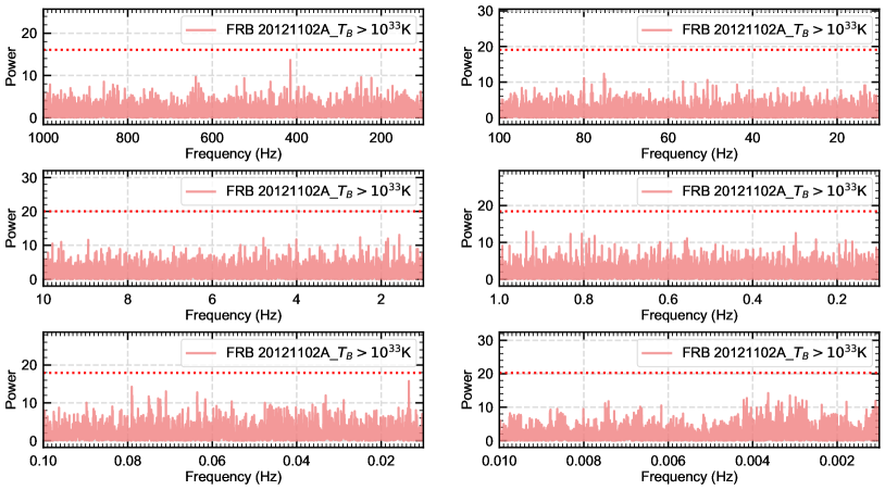
Figure 20: Periodicity analysis for FRB 20121102A based on classification according to the brightness temperature. The Schuster periodogram method is applied in the analysis. The upper six panels correspond to typical bursts with $T_{B}<10^{33}$ K, and the lower six panels correspond to the bright subset of bursts with $T_{B}>10^{33}$ K. For each subset, the whole period range of 0.001 s–1000 s is divided into 6 segments, i.e. 0.001 s–0.01 s, 0.01 s–0.1 s, 0.1 s–1 s, 1 s–10 s, 10 s–100 s, and 100 s–1000 s. The horizontal dotted line in each panel represents a coincidence level of $<10^{-5}$. No clear evidence of periodicity is found in these plots.

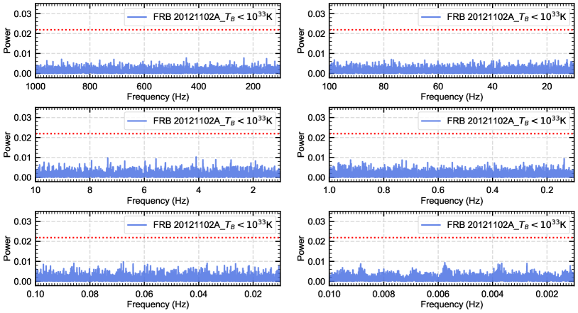
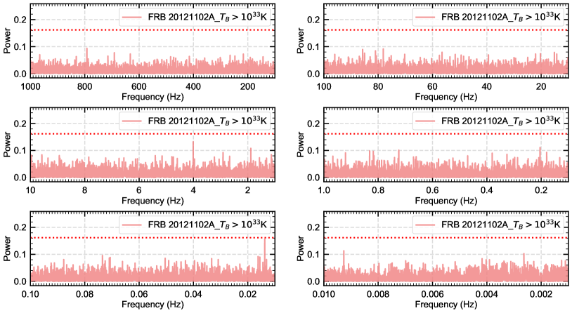
Figure 21: Periodicity analysis for FRB 20121102A based on classification according to the brightness temperature. The Lomb-Scargle periodogram method is applied in the analysis. The upper six panels correspond to typical bursts with $T_{B}<10^{33}$ K, and the lower six panels correspond to the bright subset of bursts with $T_{B}>10^{33}$ K. For each subset, the whole period range of 0.001 s–1000 s is divided into 6 segments, i.e. 0.001 s–0.01 s, 0.01 s–0.1 s, 0.1 s–1 s, 1 s–10 s, 10 s–100 s, and 100 s–1000 s. The horizontal dotted line in each panel represents a coincidence level of $<0.001$. No clear evidence of periodicity is found in these plots.

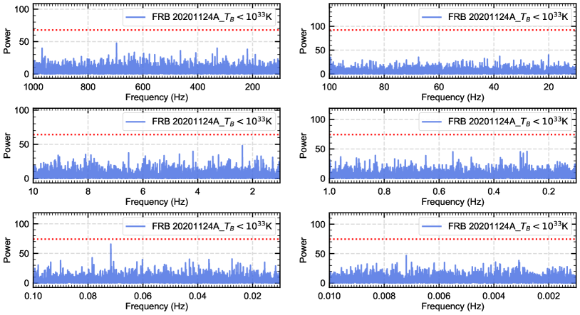
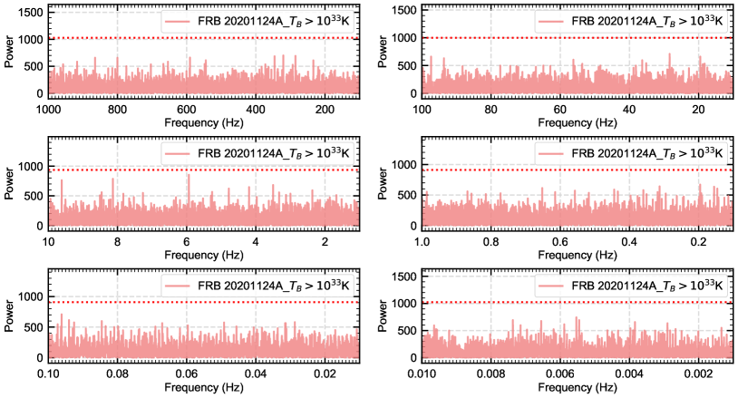
Figure 22: Periodicity analysis for FRB 20201124A based on classification according to the brightness temperature. The Schuster periodogram method is applied in the analysis. The upper six panels correspond to typical bursts with $T_{B}<10^{33}$ K, and the lower six panels correspond to the bright subset of bursts with $T_{B}>10^{33}$ K. For each subset, the whole period range of 0.001 s–1000 s is divided into 6 segments, i.e. 0.001 s–0.01 s, 0.01 s–0.1 s, 0.1 s–1 s, 1 s–10 s, 10 s–100 s, and 100 s–1000 s. The horizontal dotted line in each panel represents a coincidence level of $<10^{-5}$. No clear evidence of periodicity is found in these plots.

References

- Beniamini et al. (2020) Beniamini P., Wadiasingh Z., Metzger B. D., 2020, Monthly Notices of the Royal Astronomical Society, 496, 3390
- CHIME/FRB Collaboration et al. (2020) CHIME/FRB Collaboration et al., 2020, Nature, 582, 351
- CHIME/FRB Collaboration et al. (2021) CHIME/FRB Collaboration et al., 2021, The Astrophysical Journal Supplement Series, 257, 59
- CHIME/FRB Collaboration et al. (2022) CHIME/FRB Collaboration et al., 2022, Nature, 607, 256
- Chatterjee et al. (2017) Chatterjee S., et al., 2017, Nature, 541, 58
- Chen et al. (2021) Chen H.-Y., Gu W.-M., Sun M., Liu T., Yi T., 2021, The Astrophysical Journal, 921, 147
- Geng & Huang (2015) Geng J., Huang Y., 2015, The Astrophysical Journal, 809, 24
- Geng et al. (2021) Geng J., Li B., Huang Y., 2021, The Innovation, 2, 100152
- Hewitt et al. (2022) Hewitt D. M., et al., 2022, Monthly Notices of the Royal Astronomical Society, 515, 3577
- Hu & Huang (2023) Hu C.-R., Huang Y.-F., 2023, arXiv preprint, arXiv:2212.05242
- Ioka & Zhang (2020) Ioka K., Zhang B., 2020, The Astrophysical Journal Letters, 893, L26
- Katz (2021) Katz JI., 2021, Monthly Notices of the Royal Astronomical Society, 502, 4664
- Kirsten et al. (2022) Kirsten F., et al., 2022, Nature, 602, 585
- Kurban et al. (2022) Kurban A., et al., 2022, The Astrophysical Journal, 928, 94
- Levin et al. (2020) Levin Y., Beloborodov A. M., Bransgrove A., 2020, The Astrophysical Journal Letters, 895, L30
- Li et al. (2018) Li D., et al., 2018, IEEE Microwave Magazine, 19, 112
- Li et al. (2021a) Li CK., et al., 2021a, Nature Astronomy, 5, 378
- Li et al. (2021b) Li D., et al., 2021b, Nature, 598, 267
- Li et al. (2021c) Li Q.-C., Yang Y.-P., Wang F. Y., Xu K., Shao Y., Liu Z.-N., Dai Z.-G., 2021c, The Astrophysical Journal Letters, 918, L5
- Lomb (1976) Lomb N. R., 1976, Astrophysics and Space Science, 39, 447
- Lorimer et al. (2007) Lorimer D. R., Bailes M., McLaughlin M. A., Narkevic D. J., Crawford F., 2007, Science, 318, 777
- Marcote et al. (2017) Marcote B., et al., 2017, The Astrophysical Journal, 834, L8
- Marcote et al. (2020) Marcote B., et al., 2020, Nature, 577, 190
- Marthi et al. (2021) Marthi V. R., et al., 2021, Monthly Notices of the Royal Astronomical Society
- Mereghetti et al. (2020) Mereghetti S., et al., 2020, The Astrophysical Journal Letters, 898, L29
- Moroianu et al. (2023) Moroianu A., Wen L., James C. W., Ai S., Kovalam M., Panther F. H., Zhang B., 2023, Nature Astronomy, 7, 579
- Nimmo et al. (2023) Nimmo K., et al., 2023, Monthly Notices of the Royal Astronomical Society, 520, 2281
- Niu et al. (2022a) Niu J.-R., et al., 2022a, Research in Astronomy and Astrophysics, 22, 124004
- Niu et al. (2022b) Niu C.-H., et al., 2022b, Nature, 606, 873
- Pastor-Marazuela et al. (2021) Pastor-Marazuela I., et al., 2021, Nature, 596, 505
- Pastor-Marazuela et al. (2023) Pastor-Marazuela I., et al., 2023, Astronomy & Astrophysics, 678, A149
- Petroff et al. (2016) Petroff E., et al., 2016, Publications of the Astronomical Society of Australia, 33, e045
- Planck Collaboration et al. (2020) Planck Collaboration et al., 2020, Astronomy & Astrophysics, 641, A6
- Platts et al. (2019) Platts E., Weltman A., Walters A., Tendulkar SP., Gordin JEB., Kandhai S., 2019, Physics Reports, 821, 1
- Pleunis et al. (2021) Pleunis Z., et al., 2021, The Astrophysical Journal, 923, 1
- Rajwade et al. (2020) Rajwade KM., et al., 2020, Monthly Notices of the Royal Astronomical Society, 495, 3551
- Scargle (1982) Scargle J. D., 1982, The Astrophysical Journal, 263, 835
- Schuster (1898) Schuster A., 1898, Terrestrial Magnetism, 3, 13
- Spitler et al. (2016) Spitler LG., et al., 2016, Nature, 531, 202
- Sridhar et al. (2021) Sridhar N., Metzger B. D., Beniamini P., Margalit B., Renzo M., Sironi L., Kovlakas K., 2021, The Astrophysical Journal, 917, 13
- Tendulkar et al. (2017) Tendulkar S. P., et al., 2017, The Astrophysical Journal Letters, 834, L7
- Thornton et al. (2013) Thornton D., et al., 2013, Science, 341, 53
- Tong et al. (2020) Tong H., Wang W., Wang H.-G., 2020, Research in Astronomy and Astrophysics, 20, 142
- Xiao & Dai (2022a) Xiao D., Dai Z.-G., 2022a, Astronomy & Astrophysics, 657, L7
- Xiao & Dai (2022b) Xiao D., Dai Z.-G., 2022b, Astronomy & Astrophysics, 667, A26
- Xu et al. (2021) Xu K., Li Q.-C., Yang Y.-P., Li X.-D., Dai Z.-G., Liu J., 2021, The Astrophysical Journal, 917, 2
- Xu et al. (2022) Xu H., et al., 2022, Nature, 609, 685
- Xu et al. (2023) Xu J., et al., 2023, Universe, 9, 330
- Yang & Zou (2020) Yang H., Zou Y.-C., 2020, The Astrophysical Journal Letters, 893, L31
- Zanazzi & Lai (2020) Zanazzi JJ., Lai D., 2020, The Astrophysical Journal Letters, 892, L15
- Zhang (2020) Zhang B., 2020, Nature, 587, 45
- Zhang & Gao (2020) Zhang X., Gao H., 2020, Monthly Notices of the Royal Astronomical Society: Letters, 498, L1
- Zhang et al. (2023) Zhang Y.-K., Li D., Feng Y., Wang P., Niu C.-H., Dai S., Yao J.-M., Tsai C.-W., 2023, arXiv preprint, arXiv:2305.18052