LRRU: Long-short Range Recurrent Updating Networks for Depth Completion
– Supplementary Materials –

Abstract

In this supplementary material, we provide further details in evaluation metrics, quantitative and qualitative analysis of our iterative update process, and qualitative comparisons on the NYUv2 dataset. In addition, we adopt the proposed LRRU method in the basic framework of existing SPN-based methods to further demonstrate the advantages of our method.

1 Evaluation metrics.

Following exiting depth completion methods [MaCK19, lin2022dynamic, cheng2019cspn, cheng2020cspn++, xu2020deformable, park2020non, HuWLNFG21, lin2022dynamic, liu2022graphcspn], we employ the Root Mean Squared Error (RMSE[$\mathrm{mm}$]), Mean Absolute Error (MAE[$\mathrm{mm}$]), Root Mean Squared Error of the Inverse depth (iRMSE[1/ $\mathrm{km}$]), Mean Absolute Error of the Inverse depth (iMAE[1/$\mathrm{km}$]), mean absolute relative error (REL), and percentage of pixels satisfying $\delta_{\tau}$ for quantitative evaluation. Eq. (1) shows the detailed definitions, where $d^{gt}$ denotes the ground truth depth map, $d^{pred}$ denotes the predicted dense depth map, and $\mathcal{V}$ is the set of available points in the ground truth.

2 Analysis of Our Iterative Update Process.

In this paper, we present the Long-short Range Recurrent Updating Network (LRRU), a novel lightweight deep network framework for depth completion. Given a sparse input depth map, we first fill it to an initial dense depth map using a simple non-learning method [ku2018defense]. Then, according to the long-short range recurrent strategy, our method iteratively updates the initial depth map through the Target-Dependent Update Unit (TDU) to obtain the final accurate depth maps. Our update process is target-adaptive and highly flexible, and the proposed method only requires 4 iterations to achieve satisfactory results. In this section, we perform both qualitative and quantitative analysis on the result of the depth map during the iterative update process. The experiments are conducted on the KITTI validation dataset [Geiger2012CVPR].

$$[!t]\begin{aligned} &\operatorname{RMSE}[\mathrm{mm}]:\sqrt{\frac{1}{|\mathcal{V}|}\sum_{v\in\mathcal{V}}\left|d_{v}^{gt}-d_{v}^{pred}\right|^{2}},\\ &\operatorname{MAE}[\mathrm{mm}]:\frac{1}{|\mathcal{V}|}\sum_{v\in\mathcal{V}}\left|d_{v}^{gt}-d_{v}^{\text{pred }}\right|,\\ &\operatorname{iRMSE}[1/\mathrm{km}]:\sqrt{\frac{1}{|\mathcal{V}|}\sum_{v\in\mathcal{V}}\left|1/d_{v}^{gt}-1/d_{v}^{\text{pred }}\right|^{2}},\\ &\operatorname{iMAE}[1/\mathrm{km}]:\frac{1}{|\mathcal{V}|}\sum_{v\in\mathcal{V}}\left|1/d_{v}^{gt}-1/d_{v}^{\text{pred }}\right|,\\ &\text{ REL }:\frac{1}{|\mathcal{V}|}\sum_{v\in\mathcal{V}}\left|\left(d_{v}^{gt}-d_{v}^{pred}\right)/d_{v}^{gt}\right|,\\ &\delta_{\tau}[\%]:\max\left(\frac{d_{v}^{gt}}{d_{v}^{pred}},\frac{d_{v}^{pred}}{d_{v}^{gt}}\right)<\tau.\end{aligned}$$ (1)

2.1 Quantitative Analysis

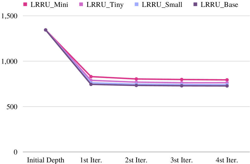
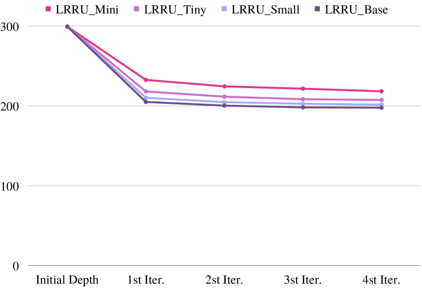
In our proposed method, the accuracy of the initial dense depth map is not strictly limited. We obtain the initial depth map by a classical handcrafted approach [ku2018defense]. Fig. 2 and Fig. 2 show the quantitative results of the depth map during the update process, which include RMSE and MAE. The experimental results demonstrate that the initial depth map is coarse, and the RMSE and MAE are 1344 mm and 299.3 mm, respectively. However, when we update the initial depth once through our Target-Dependent Update Unit (TDU), the results of the depth map are greatly enhanced. Then, as the depth map is updated iteratively, its performance is continuously improved.

2.2 Qualitative Analysis

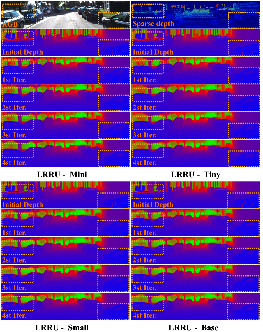
Fig. 3 shows some typical examples that demonstrate the qualitative results of the depth map during our iterative update process. As described in this paper, our proposed method employs large-to-small kernel scopes to capture long-to-short range dependencies to update the depth map. When we update the initial coarse depth map by a TDU with a large kernel scope, the structural details of the depth map are greatly improved. However, the object boundaries of the depth image are still blurred. Then, we iteratively update the depth map by TDUs with smaller kernel scopes, and the depth map continues to become more refined. Meanwhile, the experimental results demonstrate that the larger the network size of our proposed method, the finer the depth map at the same stage.

Figure 1: The RMSE [mm] change of the depth map during the iterative update process.

Figure 2: The MAE [mm] change of the depth map during the iterative update process.

3 Qualitative Comparisons on NYUv2.

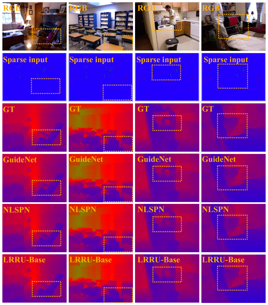
In Fig. 4, we present some depth completion results predicted by our method and other state-of-the-art (SOTA) methods, such as GuideNet [tang2019learning] and NLSPN [park2020non], on the indoor NYUv2 depth dataset. Following the previous works [MaCK19, lin2022dynamic, cheng2019cspn, cheng2020cspn++, xu2020deformable, park2020non, HuWLNFG21, lin2022dynamic, liu2022graphcspn], the sparse depth maps are obtained by randomly sampling 500 depth pixels from the dense depth maps and fed into the network with corresponding RGB images. The experimental results demonstrate that GuideNet generates blurry depth maps, as it is a direct regression method. Compared to GuideNet, the depth maps predicted by NLSPN and our method substantially improve accuracy thanks to the iterative update scheme. However, NLSPN suffers from over-smoothing problems due to massive iterations, especially on tiny or thin structures. In contrast, our method preserves tiny structures and depth boundaries well by using the proposed Target-Dependent Update Unit (TDU) and long-short range recurrent strategy.

4 LRRU using SPN framework (LRRU-SPN)

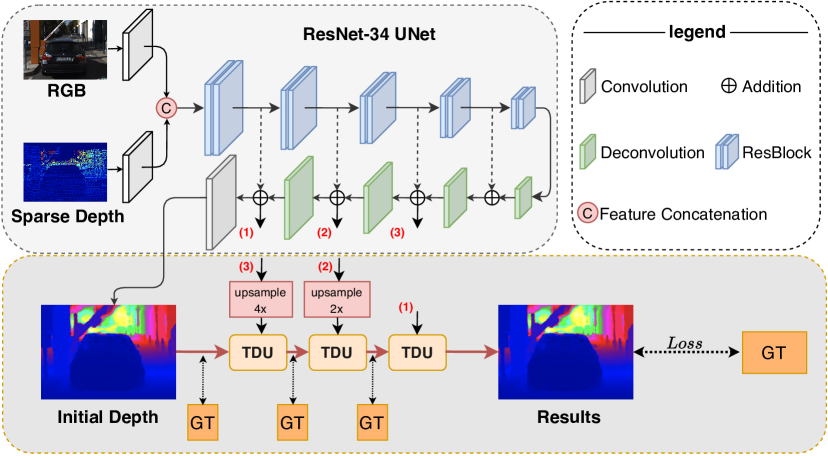
For a direct comparison with existing SPN-based methods [cheng2019cspn, cheng2020cspn++, xu2020deformable, park2020non, HuWLNFG21, lin2022dynamic, liu2022graphcspn], we adopt the proposed LRRU method in the basic framework of the SPN-based methods. We name our method LRRU-SPN with a little name misuse. As shown in Fig. 5, LRRU-SPN uses the ResNet-34 [he_ResNet_CVPR_2016] as the backbone in the same way as these SPN-based approaches. In addition, LRRU-SPN replaces the spatial propagation networks with our proposed target-dependent update unit, and iteratively employ it to update the output of the encoder-decoder network according to our long-short range recurrent strategy.

Conventional SPNs (e.g. CSPN [cheng2019cspn] and NLSPN [park2020non]) employ fixed kernel weights and scopes, which require massive iterations to obtain the long-range dependencies and decent results. By contrast, LRRU-SPN adaptively estimates the kernel weights and dynamically obtains long-to-short range dependencies by adjusting the kernel scope from large to small, which is more flexible. In this comparison experiment, we only need three iterations, where the TDUs of the update process are guided by the cross-guided features of $1/4-$scale, $1/2-$scale, and full-scale in turn. The results in Table 1 show that LRRU-SPN outperforms existing SPN-based methods and has faster inference time.

Although the process of dynamically predicting the kernel parameters will consume extra time, our method is not constrained by the number of iterations. The results on KITTI validation set show that our method using only one iteration (RMSE:741.8/time:0.07s) already outperforms NLSPN (RMSE:771.8/time:0.16s). Therefore, we consider our method to be more efficient.

Table 1: Quantitative evaluation with SPN-based methods on KTTTI test dataset. The time^∗ are from the KITTI leaderboard due to the lack of open-source code.

SPNs	Iterations	Time[s]	RMSE[mm]	MAE[mm]
CSPN [cheng2019cspn]	12	0.20s	1019.64	279.46
DSPN [xu2020deformable]	12	0.34s∗	766.74	220.36
NLSPN [park2020non]	18	0.13s	741.68	199.59
CSPN++ [cheng2020cspn++]	12	0.20s∗	743.69	209.28
DySPN [lin2022dynamic]	6	0.16s∗	709.12	192.71
GraphCSPN [liu2022graphcspn]	3	0.12s∗	736.24	193.25
LRRU-SPN	3	0.10s	707.11	202.08

Figure 3: Typical examples to demonstrate the qualitative result of the depth map during our iterative update process. Note that the sparse depth has been dilated for better visualization.

Figure 4: Qualitative comparison with SOTA methods on the NYUv2 dataset. From top to bottom are RGB images, sparse input depth maps, ground truth depth maps, dense depth maps predicted by GuideNet [tang2019learning], NLSPN [park2020non] and our LRRU-Base model, respectively. Note that the sparse input has been dilated for better visualization.

Figure 5: The network architecture of our LRRU-SPN. For a fair comparison, we employ the same network structure as the SPN-based methods. We replace the spatial propagation networks with our Target-Dependent Update Unit (TDU) and iteratively employ it to update the output of the encoder-decoder network 3 times according to the long-short range recurrent strategy.