On network dynamical systems with a nilpotent singularity

Abstract

Network dynamics is nowadays of extreme relevance to model and analyze complex systems. From a dynamical systems perspective, understanding the local behavior near equilibria is of utmost importance. In particular, equilibria with at least one zero eigenvalue play a crucial role in bifurcation analysis. In this paper, we want to shed some light on nilpotent equilibria of network dynamical systems. As a main result, we show that the blow-up technique, which has proven to be extremely useful in understanding degenerate singularities in low-dimensional ordinary differential equations, is also suitable in the framework of network dynamical systems. Most importantly, we show that the blow-up technique preserves the network structure. The further usefulness of the blow-up technique, especially with regard to the desingularization of a nilpotent point, is showcased through several examples including linear diffusive systems, systems with nilpotent internal dynamics, and an adaptive network of Kuramoto oscillators.

1 Introduction

We consider a networked system of $\displaystyle N$ scalar nodes $\displaystyle x_{i}=x_{i}(t)\in\mathbb{R}$:

$$\begin{split}\dot{x}_{i}=f_{i}(x_{i},\mu_{i})+\sum_{j=1}^{N}w_{ij}h_{ij}(x_{i},x_{j},\lambda_{ij}),\qquad i=1,\ldots,N,\end{split}$$ (1.1)

where $\displaystyle f_{i}$ and $\displaystyle h_{ij}$ are smooth functions with some “internal” parameters $\displaystyle\mu_{i}\in\mathbb{R}^{u_{i}}$, “interaction parameters” $\displaystyle\lambda_{ij}\in\mathbb{R}^{l_{ij}}$, and “weights” $\displaystyle w_{ij}\in\mathbb{R}$. We refer to $\displaystyle f_{i}$ as the internal dynamics and to $\displaystyle h_{ij}$ as the interaction. The topology of the network is encoded in $\displaystyle w_{ij}$, which are the coefficients of a weighted adjacency matrix. In compact form, we can write (1.1) as

$$\dot{x}=F(x,\mu)+H(x,w,\lambda),$$ (1.2)

where $\displaystyle F$ includes all the internal dynamics and $\displaystyle H$ all the interactions; and with $\displaystyle x\in\mathbb{R}^{N}$, $\displaystyle\mu\in\mathbb{R}^{u_{1}+\cdots+u_{N}}=\mathbb{R}^{u}$, $\displaystyle w\in\mathbb{R}^{N^{2}}$ and $\displaystyle\lambda\in\mathbb{R}^{l}$ with $\displaystyle l=\sum_{i,j=1}^{N}l_{ij}$. We shall say that a system has a network structure [26, 30, 34] if it can be (re-)written in the form (1.1), or equivalently (1.2). The main idea is that one can clearly distinguish the internal, or uncoupled, dynamics from the network interaction. In the rest of this paper, we shall concentrate on studying the dynamics near a nilpotent equilibrium point of (1.1). We recall that given a differential equation $\displaystyle\dot{x}=f(x)$, $\displaystyle x\in\mathbb{R}^{n}$, an equilibrium point $\displaystyle x^{*}$ is said to be nilpotent if the eigenvalues of the Jacobian $\displaystyle\textnormal{D}_{x}f(x^{*})$ are all zero.

The main conclusion drawn from the analysis presented in this paper is that the blow-up transformation preserves the network structure. We point out that, a priori, there is no guarantee for a coordinate change to preserve any sort of structure. This can be assessed by simply attempting a linear transformation on e.g. (1.2). The blow-up (see section 2.1) is a singular coordinate transformation that has been extensively used to desingularize the local dynamics of (mostly) low dimensional differential equations. Some further important observations are the following (for the details see section 2):

• A node-directional blow-up induces dynamics on the “blown-up” edges. However, these dynamics occur at higher orders. That is, up to leading order terms, the blown-up network is still static, see section 2.3.

• A parameter-directional blow-up is, essentially, a rescaling such that a distinguished parameter is set to $\displaystyle 1$ and the rest are kept small, see section 2.4.

• The blow-up seems to be especially useful for slowly adaptive networks, where, for example, an edge-directional blow-up leads to a static network with a distinguished edge fixed to $\displaystyle 1$. Moreover, the adaptation rule that defines the dynamics of such distinguished edge is visible, globally, in the whole network, see section 2.5.

Before going into the technical details, let us motivate our interest with some examples.

1.1 Motivating examples

In this section, we motivate considering networked systems with nilpotent equilibria through some examples.

Nilpotent internal dynamics:

Consider a weakly coupled network of the form (1.1) given by

$$\begin{split}\dot{x}_{i}=f_{i}(x_{i},\mu_{i})+\varepsilon\sum_{j=1}^{N}w_{ij}h_{ij}(x_{i},x_{j},\lambda_{ij}),\qquad i=1,\ldots,N,\end{split}$$ (1.3)

where $\displaystyle 0<\varepsilon\ll 1$, and such that there is a fixed set of parameters $\displaystyle\mu_{i}^{*}$, and a point $\displaystyle x^{*}=(x_{1}^{*},\ldots,x_{N}^{*})$, such that $\displaystyle f_{i}(x_{i}^{*},\mu_{i}^{*})=\frac{\partial f_{i}}{\partial x_{i}}(x_{i}^{*},\mu_{i}^{*})=0$. In this case, the point $\displaystyle x^{*}$ is nilpotent for $\displaystyle\varepsilon=0$ and an approach to investigate the dynamics for $\displaystyle\varepsilon$ small could be via the blow-up technique, as we shall present in this paper. See a concrete example in section 3.2.

Remark 1.

Even though we focus on networks of scalar nodes, dynamic networks with nilpotent internal dynamics frequently appear once the nodes are considered multidimensional. For example, one may consider coupled neuronal models [32] where each neuron modeled, e.g. via the Hodgkin-Huxley model or its simplifications contains nilpotent points in its internal dynamics. In a more general setting, nilpotent Hopf bifurcations have been considered for coupled cell networks [8], see also [13, 12, 24]. In such a case, an adapted version of [14] together with the blow-up analysis considered here could be applicable as well.

A class of nonlinear consensus protocols:

Consider the general consensus protocol

$$\dot{x}=-L\left(Ax+\sum_{i=2}^{p}F_{i}(x)\right),$$ (1.4)

where $\displaystyle x\in\mathbb{R}^{N}$, $\displaystyle p\geq 2$, $\displaystyle L$ is a Laplacian matrix, $\displaystyle A$ is a non-singular matrix and $\displaystyle F_{i}$ is a homogeneous polynomial vector field of degree $\displaystyle i$. The classical consensus protocol is obtained when $\displaystyle A=I$ and $\displaystyle F_{i}=0$ for all $\displaystyle i\geq 2$. On the other hand, if $\displaystyle A=0$ we immediately have that the origin is nilpotent. Furthermore, even if one simply considers $\displaystyle\dot{x}=-LF_{2}(x)$, any $\displaystyle x^{*}$ so that $\displaystyle F(x^{*})\in\ker L$ would correspond to a nilpotent point. Since the kernel of $\displaystyle L$ is non-trivial, nilpotent points become relevant in this situation. See [5] for a particular case study, and [16] for a similar, but adaptive, example.

Canceling linear dynamics:

Consider (1.1) in the particular matrix form

$$\dot{x}=Ax+Bx+\cdots,$$ (1.5)

where $\displaystyle A$ is diagonal, accounting for the (leading part of the) internal dynamics, and $\displaystyle B$ is a matrix describing the (leading part of the) interaction; the dots stand for higher-order terms. One can then realize that, upon variation of parameters, some components of these linear parts may “cancel” in the sense of having a nilpotent form. Clearly, this does not require $\displaystyle A=-B$ in general. For example, consider the homogeneous case where $\displaystyle A=aI_{N}$ with $\displaystyle a\in\mathbb{R}$. So, it suffices to notice that if $\displaystyle T$ is the (complex) matrix that brings $\displaystyle B$ into its Jordan canonical form, then the transformation $\displaystyle x\mapsto T^{-1}x$ implies $\displaystyle T(aI_{N}+B)T^{-1}=aI_{N}+J_{B}$, where $\displaystyle J_{B}$ is the Jordan canonical form of $\displaystyle B$, and is upper-triangular. In turn, $\displaystyle aI_{N}+J_{B}$ can be nilpotent, or at least have some zero eigenvalues, for $\displaystyle B\neq-A$. For an example see section 3.1, and [27] for a related scenario.

(Slowly) adaptive networks:

As in the classical (low-dimensional) setting, nilpotent singularities are extremely relevant for slow-fast systems [21, 36]. Consider the (slowly) adaptive dynamic network [3, 31]

$$\begin{split}\dot{x}_{i}&=f_{i}(x_{i},\mu_{i})+\sum_{j=1}^{N}w_{ij}h_{ij}(x_{i},x_{j},\lambda_{ij})\\ \dot{w}_{ij}&=\varepsilon g_{ij}(x,w_{ij}).\end{split}$$ (1.6)

If one were to attempt the analysis of (1.6) with techniques derived from Geometric Singular Perturbation Theory (GSPT), the nilpotent points of (1.6) restricted to $\displaystyle\varepsilon=0$ define a class of singularities nearby which the solutions may exhibit a quite intricate behavior for $\displaystyle 0<\varepsilon\ll 1$. As a particular example consider a family of adaptive Kuramoto oscillators

$$\begin{split}\phi_{i}^{\prime}&=\Omega-\frac{1}{N}\sum_{j=1}^{N}w_{ij}\sin(\phi_{i}-\phi_{j}+\alpha)\\ w_{ij}^{\prime}&=-\varepsilon\left(\sin(\phi_{i}-\phi_{j}+\beta)+w_{ij}\right),\end{split}$$ (1.7)

with parameters $\displaystyle\alpha,\beta$ close to zero. A phase-locked equilibrium is given by

$$\begin{split}\phi_{i}^{*}&=\psi_{i}\\ w_{ij}^{*}&=-\sin(\psi_{i}-\psi_{j}+\beta)\\ \Omega&=-\frac{1}{N}\sum_{j=1}^{N}\sin(\psi_{i}-\psi_{j}+\beta)\sin(\psi_{i}-\psi_{j}+\alpha),\end{split}$$ (1.8)

for some $\displaystyle\psi_{i}\in[0,2\pi)$, $\displaystyle i=1,\ldots,N$. As an example, let us take a 4-node network and $\displaystyle\psi=(\psi_{1},\psi_{2},\psi_{3},\psi_{4})=\left(0,\frac{\pi}{2},\pi,\frac{3\pi}{2}\right)$. For this choice of equilibrium phases, the phase-locked equilibrium is nilpotent for $\displaystyle\alpha=\beta=0$ and $\displaystyle\Omega=-\frac{1}{2}$. Indeed we have that the relevant part of the linearization, at the aforementioned phase-locked equilibrium, is given by

$$\begin{split}J&=\frac{1}{4}\begin{bmatrix}w_{13}&0&-w_{13}&0\\ 0&w_{24}&0&-w_{24}\\ -w_{31}&0&w_{31}&0\\ 0&-w_{42}&0&w_{42}\end{bmatrix}.\end{split}$$ (1.9)

So, further noting that $\displaystyle w_{13}^{*}=w_{31}^{*}=w_{24}^{*}=w_{42}^{*}=0$ we have that $\displaystyle J=0$, implying that the phase-locked equilibrium is nilpotent. This example is further detailed in section 3.3.

Remark 2.

Adaptivity is, of course, not necessary. See for example [33] where nilpotent equilibria of the classical Kuramoto model are considered.

As motivated in the previous examples, we are interested in network dynamical systems (1.1), equivalently (1.2), with a nilpotent singularity. Nilpotent points are highly important because they hint at the possibility of complicated bifurcations occurring in their vicinity. From now on, we shall assume that there is a set of parameters $\displaystyle\mu^{*}$, $\displaystyle\lambda^{*}$ and edge weights $\displaystyle w^{*}$ such that $\displaystyle x^{*}$ is an isolated nilpotent equilibrium point of (1.2).

Remark 3.

Assuming $\displaystyle x^{*}$ being isolated is not too strict, at least for our arguments regarding the blow-up transformation preserving the network structure, because one can also blow-up higher-dimensional sets of equilibria in a similar way. We present a brief description of the blow-up transformation and several relevant references in section 2.1.

Without loss of generality, we further assume that the nilpotent point is at $\displaystyle x^{*}=0$ for $\displaystyle(\mu^{*},\lambda^{*},\omega^{*})=(0,0,0)$. However, we emphasize that, as presented in the examples, a nilpotent point does not necessarily have to be related to a disconnected network. Let $\displaystyle a_{i}(\mu)=\frac{\partial f_{i}}{\partial x_{i}}(0,\mu)$, $\displaystyle D(\mu)=\operatorname{diag}\left\{a_{i}(\mu)\right\}_{i=1}^{N}$, and $\displaystyle A(\omega,\lambda)=\frac{\partial H}{\partial x}(0,\omega,\lambda)$. So, we can write (1.2) as

$$\dot{x}=(D(\mu)+A(\omega,\lambda))x+\tilde{F}(x,\mu)+\tilde{H}(x,w,\lambda),$$ (1.10)

where, from our assumptions, $\displaystyle D(0)+A(0,0)$ is a nilpotent matrix (and non of which needs to be the zero matrix) and $\displaystyle\tilde{F}$ and $\displaystyle\tilde{H}$ stand, respectively, for the higher-order terms (by this we mean monomials of degree higher than one) of the internal dynamics and of the interaction.

It is an important question whether one may indeed expect the leading term $\displaystyle D(\mu)+A(\omega,\lambda)$ in (1.10) to be nilpotent for parameters $\displaystyle(\mu,\omega,\lambda)=(\mu^{*},\omega^{*},\lambda^{*})$. Roughly speaking, since $\displaystyle n$ eigenvalues are required to be zero, we expect that this can be achieved, generically, for $\displaystyle n$-parameter families of dynamic networks (1.10). More formally, since $\displaystyle GL(n)$ has dimension $\displaystyle n^{2}$ and since there are at most $\displaystyle n(n-1)$ “different” nilpotent matrices, one expects that such matrices appear generically whenever $\displaystyle D(\mu)+A(\omega,\lambda)$ has at least $\displaystyle n$ independent parameters. In other words, if $\displaystyle D(\mu)+A(\omega,\lambda)$ has at least $\displaystyle n$ independent parameters, then there is at least one particular choice $\displaystyle(\mu^{*},\omega^{*},\lambda^{*})$ such that $\displaystyle D(\mu^{*})+L(\omega^{*},\lambda^{*})$ is nilpotent. Moreover, since the only nilpotent symmetric matrix is the zero matrix, we shall consider that the interaction is directed.

Remark 4.

We emphasize that we do not put $\displaystyle D(0)+A(0,0)$ in normal form since, generally speaking, a similarity transformation destroys the network structure of the system.

2 Blowing up preserves the network structure

Our aim in this section is to show that the (singular) coordinate transformation known as blow-up, when applied to a nilpotent singularity of a network dynamical system, preserves the network structure. Due to the importance of the blow-up, although the literature contains already plenty of information on it [1, 17, 21], we prefer to provide a brief recollection of what is known as a blow-up in the way it is used in this paper. More importantly, in this section, we provide certain terminology and fix some notations that are later used in the examples of section 3.

2.1 The blow-up

Let $\displaystyle X:\mathbb{R}^{n}\to\mathbb{R}^{n}$ be a smooth vector field such that $\displaystyle X(0)=0$ and $\displaystyle 0\in\mathbb{R}^{n}$ is a nilpotent point. Let $\displaystyle\phi:\mathbb{S}^{n-1}\times I\to\mathbb{R}^{n}$ be a weighted polar transformation given by

$$(\bar{x}_{1},\ldots,\bar{x}_{n},r)\mapsto(r^{\alpha_{1}}\bar{x}_{1},\ldots,r^{\alpha_{n}}\bar{x}_{n})=(x_{1},\ldots,x_{n}),$$ (2.1)

where $\displaystyle\alpha_{i}\in\mathbb{N}$ for all $\displaystyle i=1,\ldots,n$, $\displaystyle\sum_{i=1}^{n}\bar{x}_{i}^{2}=1$ (i.e. $\displaystyle(\bar{x}_{1},\ldots,\bar{x}_{n})\in\mathbb{S}^{n-1}$) and $\displaystyle r\in I\subset\mathbb{R}$ where $\displaystyle I$ is an interval containing the origin. We notice that $\displaystyle\phi^{-1}$ maps the origin $\displaystyle 0\in\mathbb{R}^{n}$ to the sphere $\displaystyle\mathbb{S}^{n-1}\times\left\{0\right\}$ and we usually say that “the origin is blown-up to a sphere”. On the other hand, $\displaystyle\phi$ is a diffeomorphism whenever $\displaystyle r>0$. Due to the weights in the transformation, one refers to the transformation as quasihomogeneous (and homogeneous when all weights are the same). These weights often facilitate the desingularization (see a description below), but their appropriate choice can be quite complicated. If the diagram of figure 1 commutes, then we call $\displaystyle\bar{X}$ the blown-up vector field.

Figure 1: Commutative diagram defining a blow-up transformation.

Since $\displaystyle X(0)=0$, it follows that $\displaystyle\bar{X}|_{r=0}=0$. However, if the weights are appropriately chosen, one can often desingularize $\displaystyle\bar{X}$ by dividing by some power of $\displaystyle r$. In other words, one can define the desingularized vector field $\displaystyle\tilde{X}=\frac{1}{r^{k}}\bar{X}$ such that $\displaystyle\tilde{X}(0)\neq 0$ and $\displaystyle\tilde{X}$ has semi-hyperbolic singularities only (and no more nilpotent ones). Recalling that $\displaystyle\phi$ is a diffeomorphism for $\displaystyle r>0$, the main advantage now is that for $\displaystyle r>0$ small (i.e. near $\displaystyle\mathbb{S}^{n-1}\times\left\{0\right\}$) one can recover the dynamics of $\displaystyle\bar{X}$ from those of $\displaystyle\tilde{X}$, and in turn these describe the dynamics of $\displaystyle X$ near the origin. In practice, however, working with spherical coordinates can become cumbersome very quickly. Hence, one prefers to work with directional blow-ups, which are defined by replacing $\displaystyle\mathbb{S}^{n-1}$ by its charts. Moreover, blowing up using a sphere is not necessary, as one can blow-up, for example, to a hyperbolic manifold [22].

Although the origins of the blow-up transformation are in algebraic geometry, the blow-up transformation has proven extremely useful in dynamical systems to study nilpotent singularities. It has been, for example, used to study degenerate bifurcation problems and their unfoldings [35, 6], see also the survey [1]; or, of particular relevance for this paper, to study some non-hyperbolic points of slow-fast systems [7, 20], see also the survey [17]. Indeed, in the aforementioned context, one can consider nowadays that the blow-up transformation is a standard tool of Geometric Singular Perturbation Theory [21, 36]. Over the past decades, the blow-up transformation has been mostly used for low-dimensional problems. In fact, it is known that analytic vector fields up to dimension three can be desingularized after a finite number of blow-ups [28, 29]. In this paper, we will see the usefulness of the blow-up transformation on systems that are usually considered large-dimensional, dynamic networks. As dynamic networks are, usually, of large dimension, a relevant direction in this regard is the blow-up in the context of PDEs [15, 19, 10, 9], which so far has been considered without networks structure and, in some cases, can be regarded as mean-field limits of dynamic networks [23, 11].

2.2 Structure preservation

This section is dedicated to showing that a general directional blow-up preserves the network structure of a given dynamical system.

Remark 5.

As described in the previous section, usually one expects that after desingularization via blow-up one gains a certain degree of hyperbolicity. The number of blow-up transformations to completely desingularize a nilpotent singularity is, however, not known a priori. This means that, after a blow-up, some of the new singularities may be semi-hyperbolic or (even still) nilpotent. This is nevertheless already good progress. In the former case, further analysis can be restricted to a lower dimensional subset, the corresponding center manifold, where the blow-up can be applied again. In the latter, the process of blowing-up can also be repeated in a system that is, usually, less degenerate than the starting one. Nevertheless, one expects that after a finite number of blow-ups, one can fully describe the dynamics of a system near a nilpotent singularity.

We emphasize that in this section, we only focus on structure preservation via blowing up. The question of (full) desingularization is a nontrivial one and is highly dependent on the particular problem at hand, and the choice of weights in the quasihomogeneous blow-up (a nontrivial task in itself). We discuss some cases where one can achieve desingularization later in the examples of section 3.

Using the notation introduced above, let us consider a vector field of the form

$$X:\left\{\begin{aligned} \dot{x}&=F(x,\sigma)+H(x,\sigma)=(D_{\sigma}+A_{\sigma})x+\tilde{F}(x,\sigma)+\tilde{H}(x,\sigma)\\ \dot{\sigma}&=0,\end{aligned}\right.$$ (2.2)

where $\displaystyle F$ stands for the internal dynamics, $\displaystyle H$ the interaction, and $\displaystyle\sigma\in\mathbb{R}^{p}$ includes all possible parameters, hence $\displaystyle D_{0}+A_{0}$ is nilpotent. Our objective is to show that a local vector field obtained by a directional blow-up has the same identifiable structure of internal dynamics plus interaction.

Remark 6.

The blow-up technique is local. Hence, without further mentioning it, we assume that the vector fields we are considering are polynomial.

Let us define a quasihomogeneous blow-up via the map $\displaystyle\Xi:\mathbb{R}_{\geq 0}\times\mathbb{S}^{N+p-1}\to\mathbb{R}^{N+p}$ given by:

$$\Xi:(r,\bar{x}_{1},\ldots,\bar{x}_{n},\bar{\sigma}_{1},\ldots,\bar{\sigma}_{p})\mapsto\underbrace{(r^{\alpha_{1}}\bar{x}_{1},\dots,r^{\alpha_{n}}\bar{x}_{n},r^{\beta_{1}}\bar{\sigma}_{1},\ldots,r^{\beta_{p}}\bar{\sigma}_{p})}_{=(x_{1},\ldots,x_{N},\sigma_{1},\ldots,\sigma_{p})},$$ (2.3)

and where

$$\sum_{i=1}^{N}\bar{x}_{i}^{2}+\sum_{j=1}^{p}\bar{\sigma}_{j}^{2}=1.$$ (2.4)

We can define a directional blow-up by fixing one of the blown-up variables in $\displaystyle\mathbb{S}^{N+p-1}$ to $\displaystyle\pm 1$ and let the rest be coordinates in $\displaystyle\mathbb{R}^{n-1}$ (this is, of course, reminiscent of a stereographic projection). The sign is, for now, rather inessential, so let us consider charts

$$\begin{split}K_{i}&=\left\{\bar{x}_{i}=1\right\},\qquad i=1,\ldots,N\\ Q_{j}&=\left\{\bar{\sigma}_{j}=1\right\},\qquad j=1,\ldots,p.\end{split}$$ (2.5)

Let us denote a corresponding directional blow-up by

$$\begin{split}\Phi_{i}&=\Xi|_{\bar{x}_{i}=1},\\ \Psi_{j}&=\Xi|_{\bar{\sigma}_{j}=1}.\end{split}$$ (2.6)

The blown-up vector field in the chart $\displaystyle K_{i}$ (resp. $\displaystyle Q_{j}$) is then obtained via the application of the corresponding change of coordinates $\displaystyle\Phi_{i}$ (resp. $\displaystyle\Psi_{j}$). For convenience, let

$$\begin{split}\bar{X}_{i}&=(\textnormal{D}\Phi_{i})^{-1}X\circ\Phi_{i},\qquad i=1,\ldots,N\\ \bar{Y}_{j}&=(\textnormal{D}\Psi_{j})^{-1}X\circ\Psi_{j},\qquad j=1,\ldots,p.\end{split}$$ (2.7)

Remark 7.

• The quasi-homogeneous blow-up requires a careful choice of weights so that the local vector fields are well defined. In this section, however, we are only interested in the form the blown-up vector fields take and hence assume that (2.7) are all well defined, especially at $\displaystyle r=0$ (possibly after a division by some power of $\displaystyle r$).

• $\displaystyle\Phi_{i}$ corresponds to a blow-up of the node $\displaystyle x_{i}$. Hence, within the context of networks, we refer to it as a “node blow-up”. On the other hand, the need to blow-up in the direction of a parameter arises when such a parameter is responsible for some singular behavior, for example when it induces a nilpotent singularity. So, if for example, $\displaystyle\sigma_{k}$ corresponds to some “weight parameter” $\displaystyle w_{ij}$, we shall refer to $\displaystyle\Psi_{k}$ as an “edge blow-up”. Of course, everything that we will present below can be extended to network dynamical systems given by

  $$\begin{split}\dot{x}_{i}&=f_{i}+\sum_{j=1}^{N}w_{ij}h_{ij},\\ \dot{w}_{ij}&=g_{ij},\end{split}$$ (2.8)

  where the “edge-directional blow-up” would be more apparent. This consideration is, however, inessential for the purposes of the paper, which is to show the preservation of the network structure after the blow-up. See more details in section 2.5.

Since the compositions $\displaystyle X\circ\Phi_{i}$ and $\displaystyle X\circ\Psi_{j}$ do not change the network structure, we only need to look at the effect of pre-multiplication by the inverse of the derivative of the directional blow-up.

2.3 Node directional blow-up

We first focus on the node blow-up, that is on the $\displaystyle\bar{X}_{i}$’s. For convenience and simplicity of the exposition, for each $\displaystyle i=1,\ldots,N$ let us reorder the components of $\displaystyle X$ according to the coordinates

$$(x_{i},x_{1},\ldots,x_{i-1},x_{i+1},\ldots,x_{N},\sigma_{1},\ldots,\sigma_{p}).$$

We call such a vector filed $\displaystyle X_{i}$, but notice that we are simply swapping the position of the $\displaystyle i$-th component. In this way the corresponding directional blow-up $\displaystyle\Phi_{i}$ is given in coordinate form by

$$\begin{pmatrix}r^{\alpha_{i}}\\ r^{\alpha_{1}}\bar{x}_{1}\\ \vdots\\ r^{\alpha_{i-1}}\bar{x}_{i-1}\\ r^{\alpha_{i+1}}\bar{x}_{i+1}\\ \vdots\\ r^{\alpha_{N}}\bar{x}_{N}\\ r^{\beta_{1}}\bar{\sigma}_{1}\\ \vdots\\ r^{\beta_{p}}\bar{\sigma}_{p}\end{pmatrix}=\begin{pmatrix}x_{i}\\ x_{1}\\ \vdots\\ x_{i-1}\\ x_{i+1}\\ \vdots\\ x_{N}\\ \sigma_{1}\\ \vdots\\ \sigma_{p}\end{pmatrix},$$ (2.9)

and therefore

$$\textnormal{D}\Phi_{i}=\begin{bmatrix}\rho_{i}&0_{1\times(N-1)}&0_{1\times p}\\ \chi_{i}&R_{i}&0_{(N-1)\times p}\\ \zeta&0_{p\times(N-1)}&B\end{bmatrix}$$ (2.10)

where

$$\begin{split}\rho_{i}&=\alpha_{i}r^{\alpha_{i}-1},\\ \chi_{i}&=(\alpha_{1}r^{\alpha_{1}-1}\bar{x}_{1},\cdots,\alpha_{i-1}r^{\alpha_{i-1}-1}\bar{x}_{i-1},\alpha_{i+1}r^{\alpha_{i+1}-1}\bar{x}_{i+1},\cdots,\alpha_{N}r^{\alpha_{N}-1}\bar{x}_{N})^{\top},\\ R_{i}&=\operatorname{diag}\left\{r^{\alpha_{1}},\cdots,r^{\alpha_{i-1}},r^{\alpha_{i+1}},\cdots,r^{\alpha_{N}}\right\},\\ \zeta&=(\beta_{1}r^{\beta_{1}-1},\cdots,\beta_{p}r^{\beta_{p}-1}\bar{\sigma}_{p})^{\top},\\ B&=\operatorname{diag}\left\{r^{\beta_{1}},\cdots,r^{\beta_{p}}\right\}.\end{split}$$ (2.11)

Since $\displaystyle\textnormal{D}\Phi_{i}$ is lower triangular, its inverse is also lower triangular. In fact, we have:

$$(\textnormal{D}\Phi)^{-1}=\frac{1}{\rho_{i}}\begin{bmatrix}1&0_{1\times(N-1)}&0_{1\times p}\\ -R_{i}^{-1}\chi_{i}&\rho_{i}R_{i}^{-1}&0_{(N-1)\times p}\\ -B^{-1}\zeta&0_{p\times(N-1)}&\rho_{i}B^{-1}.\end{bmatrix}$$ (2.12)

Remark 8.

As expected, $\displaystyle\textnormal{D}\Phi$ is invertible for $\displaystyle r\neq 0$.

Thus, the local vector field $\displaystyle\bar{X}_{i}=(\textnormal{D}\Phi_{i})^{-1}X_{i}\circ\Phi_{i}$ can be written in local coordinates as

$$\bar{X}_{i}:\begin{cases}r^{\prime}&=\frac{r^{1-\alpha_{i}}}{\alpha_{i}}\left(\bar{f}_{i}+\bar{h}_{i}\right),\\ \bar{x}_{k}^{\prime}&=\frac{1}{r^{\alpha_{k}}}\left(\bar{f}_{k}+\bar{h}_{k}-\frac{\alpha_{k}}{\alpha_{i}}r^{\alpha_{k}-\alpha_{i}}\bar{x}_{k}(\bar{f}_{i}+\bar{h}_{i})\right),\\ \bar{\sigma}_{j}^{\prime}&=-\frac{\beta_{j}}{\alpha_{i}}r^{-\alpha_{i}}\bar{\sigma}_{j}(\bar{f}_{i}+\bar{h}_{i}),\end{cases}$$ (2.13)

where $\displaystyle k=1,\ldots,i-1,i+1,\ldots,N$, $\displaystyle j=1,\ldots,p$ and where $\displaystyle\bar{f}_{\ell}$ and $\displaystyle\bar{h}_{\ell}$ are the $\displaystyle\ell$-th component of $\displaystyle F\circ\Phi_{i}$ and $\displaystyle H\circ\Phi_{i}$ respectively. Notice already that the equations for $\displaystyle\bar{x}_{k}$ keep, in some sense to be detailed below, the network structure.

Let $\displaystyle[M]_{ij}$ denote the $\displaystyle i,j$ entry of the matrix $\displaystyle M$. Recall from (1.10) that $\displaystyle F+H=(D_{\sigma}+A_{\sigma})x+\cdots$. This implies that, up to leading order terms, we have:

$$\begin{split}\bar{f}_{i}+\bar{h}_{i}&=(a_{i}(r^{\beta}\bar{\sigma})+[A_{r^{\beta}\bar{\sigma}}]_{ii})r^{\alpha_{i}}+\sum_{\begin{subarray}{c}j=1\\ j\neq i\end{subarray}}^{N}[A_{r^{\beta}\bar{\sigma}}]_{ij}r^{\alpha_{j}}\bar{x}_{j}+\cdots\\ \bar{f}_{k}+\bar{h}_{k}&=[A_{r^{\beta}\bar{\sigma}}]_{ki}r^{\alpha_{i}}+(a_{k}(r^{\beta}\bar{\sigma})+[A_{r^{\beta}\bar{\sigma}}]_{kk})r^{\alpha_{k}}\bar{x}_{k}+\sum_{\begin{subarray}{c}j=1\\ j\neq i\\ j\neq k\end{subarray}}^{N}[A_{r^{\beta}\bar{\sigma}}]_{kj}r^{\alpha_{j}}\bar{x}_{j}+\cdots,\end{split}$$ (2.14)

which hints to the choice of the blow-up weights $\displaystyle\alpha_{i}=\alpha$ for all $\displaystyle i=1,\dots,N$ so that every local vector field $\displaystyle\bar{X}_{i}$ is well defined for $\displaystyle r=0$. Under such a choice we have, up to leading order terms, the blown-up vector field $\displaystyle\bar{X}_{i}$ given by:

$$\begin{split}r^{\prime}&=\frac{r}{\alpha}\left((a_{i}(r^{\beta}\bar{\sigma})+[A_{r^{\beta}\bar{\sigma}}]_{ii})+\sum_{\begin{subarray}{c}j=1\\ j\neq i\end{subarray}}^{N}[A_{r^{\beta}\bar{\sigma}}]_{ij}\bar{x}_{j}+\cdots\right)\\ \bar{x}_{k}^{\prime}&=\left([A_{r^{\beta}\bar{\sigma}}]_{ki}+(a_{k}(r^{\beta}\bar{\sigma})+[A_{r^{\beta}\bar{\sigma}}]_{kk})\bar{x}_{k}+\sum_{\begin{subarray}{c}j=1\\ j\neq i\\ j\neq k\end{subarray}}^{N}[A_{r^{\beta}\bar{\sigma}}]_{kj}\bar{x}_{j}+\cdots\right)\\ &\qquad-\bar{x}_{k}\left((a_{i}(r^{\beta}\bar{\sigma})+[A_{r^{\beta}\bar{\sigma}}]_{ii})+\sum_{\begin{subarray}{c}j=1\\ j\neq i\end{subarray}}^{N}[A_{r^{\beta}\bar{\sigma}}]_{ij}\bar{x}_{j}+\cdots\right)\\ \bar{\sigma}_{j}^{\prime}&=-\frac{\beta_{j}}{\alpha}\bar{\sigma}_{j}\left((a_{i}(r^{\beta}\bar{\sigma})+[A_{r^{\beta}\bar{\sigma}}]_{ii})+\sum_{\begin{subarray}{c}j=1\\ j\neq i\end{subarray}}^{N}[A_{r^{\beta}\bar{\sigma}}]_{ij}\bar{x}_{j}+\cdots\right).\end{split}$$ (2.15)

For $\displaystyle r=0$ we have that $\displaystyle r^{\prime}=0$ and

$$\begin{split}\bar{x}_{k}^{\prime}&=[A_{0}]_{ki}+(a_{k}(0)+[A_{0}]_{kk}-a_{i}(0)-[A_{0}]_{ii})\bar{x}_{k}+\sum_{\begin{subarray}{c}j=1\\ j\neq i\\ j\neq k\end{subarray}}^{N}[A_{0}]_{kj}\bar{x}_{j}+\mathcal{O}(|\bar{x}|^{2})\\ \bar{\sigma}_{j}^{\prime}&=-\frac{\beta_{j}}{\alpha}\left(a_{i}(0)+[A_{0}]_{ii}\right)\bar{\sigma}_{j}+\mathcal{O}(\bar{\sigma}_{j}\bar{x}),\end{split}$$ (2.16)

where $\displaystyle k=1,\ldots,i-1,i+1,\ldots,N$. We can see that the blown-up system (2.15) has “dynamic” parameters $\displaystyle\bar{\sigma}$. However, for $\displaystyle r=0$ (i.e. (2.16)) the network is static. Moreover, we see that the equilibrium point of $\displaystyle\bar{x}^{\prime}$ may not be at the origin any more.

Interpretation:

one can give several network interpretations to the equation for $\displaystyle\bar{x}^{\prime}$ in (2.16). For this, it is convenient to rewrite the first part of (2.16) as

$$\bar{x}_{k}^{\prime}=[A_{0}]_{ki}+(a_{k}(0)-a_{i}(0)-[A_{0}]_{ii})\bar{x}_{k}+\sum_{\begin{subarray}{c}j=1\\ j\neq i\end{subarray}}^{N}[A_{0}]_{kj}\bar{x}_{j}+\cdots,$$ (2.17)

where we can notice a network with $\displaystyle N-1$ nodes $\displaystyle(\bar{x}_{1},\ldots,\bar{x}_{i-1},\bar{x}_{i+1},\ldots,\bar{x}_{N})$.

• As a first interpretation, one may say that the internal dynamics are now modified (“shifted” by $\displaystyle[A_{0}]_{ki}$ and “scaled” by $\displaystyle[A_{0}]_{ii}$) by the influence of node $\displaystyle i$ (which has been blown-up and “does not exists anymore”). Regarding the interaction, that remains the same, except that the node $\displaystyle i$ does not appear anymore.

• Another interpretation could be given when we re-write (2.16) as:

  $$\bar{x}_{k}^{\prime}=[A_{0}]_{ki}+a_{k}(0)\bar{x}_{k}+\sum_{\begin{subarray}{c}j=1\\ j\neq i\end{subarray}}^{N}[\tilde{A}_{0}]_{kj}\bar{x}_{j}+\cdots,$$ (2.18)

  where $\displaystyle[\tilde{A}_{0}]_{kj}=-a_{i}(0)-[L_{0}]_{ii}+[A_{0}]_{kk}$ if $\displaystyle j=k$ and $\displaystyle[\tilde{A}_{0}]_{kj}=[A_{0}]_{kj}$ otherwise. This, instead can be interpreted as the “self-interaction” having been modified by the (nonexistent) node $\displaystyle i$, while the term $\displaystyle[A_{0}]_{ki}$ can be regarded as a constant input, which is nonzero if and only if there is a connection from node $\displaystyle i$ to node $\displaystyle k$.

Finally, if $\displaystyle r=0$ is hyperbolic in the $\displaystyle r$-direction (which would be the case under desingularization), then we expect that (2.15) is a regular perturbation of (2.16) for $\displaystyle r>0$ sufficiently small. This means that the dynamics of (2.2) in a small neighborhood of the nilpotent origin can be determined from to those of (2.16), see a relevant example in section 3.

2.4 Parameter directional blow-up

We now turn our attention to the blow-up in the parameter direction (the $\displaystyle\bar{Y}_{i}$’s in (2.7)). For convenience, let us recall that we are considering the (extended) vector field

$$X:\left\{\begin{aligned} \dot{x}&=F(x,\sigma)+H(x,\sigma)=(D_{\sigma}+L_{\sigma})x+\tilde{F}(x,\sigma)+\tilde{H}(x,\sigma)\\ \dot{\sigma}&=0,\end{aligned}\right.$$ (2.19)

where $\displaystyle L_{0}+D_{0}$ is nilpotent. If one would rewrite (2.19) as $\displaystyle X=\sum_{i=1}^{N}f_{i}\frac{\partial}{\partial x_{i}}+\sum_{j=1}^{p}0\frac{\partial}{\partial\sigma_{j}}$, it is rather convenient to consider the vector field

$$Y_{j}=0\frac{\partial}{\partial\sigma_{j}}+\sum_{i=1}^{N}f_{i}\frac{\partial}{\partial x_{i}}+\sum_{k=1,\,k\neq j}^{p}0\frac{\partial}{\partial\sigma_{k}},$$ (2.20)

with the directional blow-up $\displaystyle\Psi_{j}$ given by local coordinates:

$$\begin{pmatrix}r^{\beta_{j}}\\ r^{\alpha}\bar{x}_{1}\\ \vdots\\ r^{\alpha}\bar{x}_{N}\\ r^{\beta_{1}}\bar{\sigma}_{1}\\ \vdots\\ r^{\beta_{j-1}}\bar{\sigma}_{j-1}\\ r^{\beta_{j+1}}\bar{\sigma}_{j+1}\\ \vdots\\ r^{\beta_{p}}\bar{\sigma}_{p}\end{pmatrix}=\begin{pmatrix}\sigma_{j}\\ x_{1}\\ \vdots\\ x_{N}\\ \sigma_{1}\\ \vdots\\ \sigma_{j-1}\\ \sigma_{j+1}\\ \vdots\\ \sigma_{p}\end{pmatrix}.$$ (2.21)

Recall that from the previous section we have already chosen the blow-up weights $\displaystyle\alpha_{i}=\alpha$ for all $\displaystyle i=1,\ldots,N$. Therefore

$$\textnormal{D}\Psi_{j}=\begin{bmatrix}\rho_{j}&0_{1\times N}&0_{1\times(p-1)}\\ \chi&R&0_{N\times(p-1)}\\ \zeta_{j}&0_{(p-1)\times N}&B_{j}\end{bmatrix},$$ (2.22)

where

$$\begin{split}\rho_{j}&=\beta_{j}\bar{\sigma}_{j}^{\beta_{j}-1}\\ \chi&=(\alpha r^{\alpha-1}\bar{x}_{1},\ldots,\alpha r^{\alpha-1}\bar{x}_{N})^{\top}\\ R&=\operatorname{diag}\left\{r^{\alpha},\ldots,r^{\alpha}\right\}\\ \zeta_{j}&=(\beta_{1}r^{\beta_{1}-1}\bar{\sigma}_{1},\ldots,\beta_{j-1}r^{\beta_{j-1}-1}\bar{\sigma}_{j-1},\beta_{j+1}r^{\beta_{j+1}-1}\bar{\sigma}_{j+1},\ldots,\beta_{p}r^{\beta_{p}-1}\bar{\sigma}_{p})^{\top}\\ B_{j}&=\operatorname{diag}\left\{r^{\beta_{1}},\ldots,r^{\beta_{j-1}},r^{\beta_{j+1}},\ldots,r^{\beta_{p}}\right\}.\end{split}$$ (2.23)

Following similar steps as in the previous section, we find that the corresponding local vector field (in the chart $\displaystyle Q_{j}$) reads as

$$\bar{Y}_{j}=\begin{cases}r^{\prime}&=0\\ \bar{x}_{i}^{\prime}&=\frac{1}{r^{\alpha}}(\bar{f}_{i}+\bar{h}_{i})\\ \bar{\sigma}_{k}^{\prime}&=0,\end{cases}$$ (2.24)

where $\displaystyle k=1,\ldots,j-1,j+1,\ldots,p$, and $\displaystyle\bar{f}_{\ell}$ and $\displaystyle\bar{h}_{\ell}$ are the $\displaystyle\ell$-th component of $\displaystyle F\circ\Psi_{j}$ and $\displaystyle H\circ\Psi_{j}$ respectively. Again, it is evident that the blown-up vector field $\displaystyle\bar{Y}_{j}$ still has a network structure. More specifically we have:

$$\begin{split}\bar{f}_{i}&=a_{i}(r^{\beta}\bar{\sigma})r^{\alpha}\bar{x}_{i}+\mathcal{O}(r^{2\alpha})\\ \bar{h}_{i}&=\sum_{k=1}^{N}[A_{r^{\beta}\bar{\sigma}}]r^{\alpha}\bar{x}_{k}+\mathcal{O}(r^{2\alpha}).\end{split}$$ (2.25)

We recall that in the chart $\displaystyle Q_{j}$ we use the short-hand notation

$$r^{\beta}\bar{\sigma}=(r^{\beta_{1}}\bar{\sigma}_{1},\ldots,r^{\beta_{j-1}}\bar{\sigma}_{j-1},r^{\beta_{j}},r^{\beta_{j+1}}\bar{\sigma}_{j+1},\ldots,r^{\beta_{p}}\bar{\sigma}_{p}).$$

Interpretation:

in this case the blow-up is essentially a rescaling, where one wants to focus on the influence of the particular parameter $\displaystyle\sigma_{j}$. After successful desingularization (which depends on the vector fields and the choice of blow-up weights), the blown-up vector field $\displaystyle\bar{Y}_{j}$ is, qualitatively speaking, $\displaystyle Y_{j}$ with the parameter $\displaystyle\bar{\sigma}_{j}=1$ (or $\displaystyle\bar{\sigma}_{j}=-1$ depending on the direction of the blow-up). See the example in section 3.3.

From the above insight, since a parameter $\displaystyle\sigma_{i}\in\sigma$ could be an edge weight, and due to its relevance in applied sciences, we now discuss the edge-directional blow-up in the context of adaptive networks.

2.5 Edge-directional blow-up for adaptive networks

Let us now consider a slowly adaptive network

$$\begin{split}\dot{x}_{i}&=f_{i}(x_{i})+\sum_{j=1}^{N}w_{ij}h_{ij}(x_{i},x_{j})\\ \dot{w}_{ij}&=\varepsilon g_{ij}(x,w_{ij}).\end{split}$$ (2.26)

Remark 9.

Frequently, the adaptation rule $\displaystyle g_{ij}$ in applications depends only on the nodes $\displaystyle(i,j)$, see e.g. [3]; but for our purposes such specification is not relevant.

Consider an edge-directional blow-up for the edge $\displaystyle(k,l)$ (for simplicity we only consider the positive direction)

$$x_{i}=r\bar{x}_{i},\,w_{ij}=r\bar{w}_{ij},\,\varepsilon=r\bar{\varepsilon},\,w_{kl}=r,\qquad ij\neq kl.$$ (2.27)

Remark 10.

In this section, we only focus on the preservation of network structure and its interpretation. If more details are known from the particular functions in (2.26), then a more appropriate choice of blow-up (2.27) can be made.

The corresponding blown-up system reads as:

$$\begin{split}\dot{r}&=r\bar{\varepsilon}\bar{g}_{kl}(r,\bar{x})\\ \dot{\bar{x}}_{i}&=\frac{\bar{f}_{i}(r,\bar{x}_{i})}{r}+\sum_{j=1}^{N}\bar{w}_{ij}\bar{h}_{ij}(r,\bar{x}_{i},\bar{x}_{j})-\bar{\varepsilon}\bar{x}_{i}\bar{g}_{kl}(r,\bar{x}),\qquad i\neq k\\ \dot{\bar{x}}_{k}&=\frac{\bar{f}_{k}(r,\bar{x}_{k})}{r}+\sum_{j=1,j\neq l}^{N}\bar{w}_{kj}\bar{h}_{kj}(r,\bar{x}_{k},\bar{x}_{j})+\bar{h}_{kl}(r,\bar{x}_{k},\bar{x}_{l})-\bar{\varepsilon}\bar{x}_{k}\bar{g}_{kl}(r,\bar{x}),\\ \dot{\bar{w}}_{ij}&=\bar{\varepsilon}(\bar{g}_{ij}(r,\bar{x},\bar{w}_{ij})-\bar{w}_{ij}\bar{g}_{kl}(r,\bar{x})),\quad ij\neq kl\\ \dot{\bar{\varepsilon}}&=-\bar{\varepsilon}^{2}\bar{g}_{kl}(r,\bar{x})\end{split}$$ (2.28)

The dynamics restricted to the invariant subset $\displaystyle\left\{\bar{\varepsilon}=0\right\}$ are often useful. One accordingly has that (2.28) reduces to

$$\begin{split}\dot{r}&=0\\ \dot{\bar{x}}_{i}&=\frac{\bar{f}_{i}(r,\bar{x}_{i})}{r}+\sum_{j=1}^{N}\bar{w}_{ij}\bar{h}_{ij}(r,\bar{x}_{i},\bar{x}_{j}),\qquad i\neq k\\ \dot{\bar{x}}_{k}&=\frac{\bar{f}_{k}(r,\bar{x}_{k})}{r}+\sum_{j=1,j\neq l}^{N}\bar{w}_{kj}\bar{h}_{kj}(r,\bar{x}_{k},\bar{x}_{j})+\bar{h}_{kl}(r,\bar{x}_{k},\bar{x}_{l}),\\ \dot{\bar{w}}_{ij}&=0,\quad ij\neq kl\\ \end{split}$$ (2.29)

which is the model of a static network, with weights $\displaystyle\bar{w}_{ij}$ and fixed weight $\displaystyle\bar{w}_{kl}=1$. If $\displaystyle\bar{\varepsilon}$ remains small, then (2.28) can be interpreted as a small perturbation of the static model (2.29). In this case, we notice that the weights $\displaystyle\bar{w}_{ij}$, $\displaystyle ij\neq kl$, would evolve slowly, while $\displaystyle\bar{w}_{kl}$ is still fixed to $\displaystyle 1$. Moreover, we notice that the adaptation effects of $\displaystyle w_{kl}$ are “globally transported” to the dynamics of the nodes. This may have important applications to elucidate the influence of certain edges on the rest of the network. If (2.29) has been desingularized, then the perturbation (2.28) would be regular.

3 Examples

In this section, we present several examples that highlight the use of the blow-up for network dynamical systems. In particular, we focus on network structure preservation and the possibility of desingularization after blow-up.

3.1 Linearly Diffusive systems

Our first example concerns a set of diffusively coupled nodes with linear internal dynamics:

$$\dot{x}_{i}=a_{i}x_{i}+\sum_{j=1}^{N}w_{ij}(x_{j}-x_{i}),$$ (3.1)

with parameters $\displaystyle a_{i}\in\mathbb{R}$, $\displaystyle a_{i}\neq 0$, and $\displaystyle w_{ij}\in\mathbb{R}$ such that the origin is nilpotent. For the moment, we focus on describing the flow near the origin with the parameters fixed.

To start, let us consider the case where $\displaystyle N=2$, that is:

$$\begin{split}\dot{x}_{1}&=a_{1}x_{1}+w_{12}(x_{2}-x_{1})\\ \dot{x}_{2}&=a_{2}x_{2}+w_{21}(x_{1}-x_{2}).\end{split}$$ (3.2)

For this, the nilpotency condition is given by the two simultaneous equations

$$\begin{split}a_{1}-w_{12}+a_{2}-w_{21}&=0\\ a_{1}a_{2}-a_{1}w_{21}-a_{2}w_{12}&=0.\end{split}$$ (3.3)

Notice that for these equations to have a nontrivial solution it is necessary that $\displaystyle w_{12}\neq w_{21}$ and $\displaystyle a_{1}\neq a_{2}$ which is fulfilled, generically, by having (at least) two independent parameters. Assuming that $\displaystyle a_{1},a_{2}$ are independent, we have that $\displaystyle w_{ij}=w_{ij}^{*}:=\frac{a_{i}^{2}}{a_{i}-a_{j}}$, makes the origin nilpotent.

Consider the node-directional blow-up

$$x_{1}=\pm r,\;x_{2}=r\bar{x}_{2},$$ (3.4)

where the $\displaystyle\pm$ sign accounts for the charts $\displaystyle K_{1}^{\pm}:\left\{\bar{x}_{1}=\pm 1\right\}$, and which leads to the local vector field

$$\begin{split}r^{\prime}&=r\left(a_{1}\pm w_{12}(\bar{x}_{2}\mp 1)\right)\\ \bar{x}_{2}^{\prime}&=\pm w_{21}+\bar{x}_{2}(-a_{1}+a_{2}+w_{12}-w_{21}\mp w_{12}\bar{x}_{2}),\end{split}$$ (3.5)

whereby substituting $\displaystyle w_{ij}=w_{ij}^{*}=\frac{a_{i}^{2}}{a_{i}-a_{j}}$ we get

$$\begin{split}r^{\prime}&=-\frac{a_{1}r}{a_{1}-a_{2}}(a_{2}\mp a_{1}\bar{x}_{2})\\ \bar{x}_{2}^{\prime}&=\mp\frac{(a_{2}\mp a_{1}\bar{x}_{2})^{2}}{a_{1}-a_{2}}.\end{split}$$ (3.6)

The equilibrium point of (3.6), namely $\displaystyle(r,x_{2})=(0,\pm\frac{a_{2}}{a_{1}})$, is still nilpotent, and in fact the linearization matrix at the equilibrium point is the zero matrix. However, as a slight advantage, (3.6) is in triangular form and can be desingularized to find the classification shown in figure 2.

Figure 2: Classification of the flow of the blown-up system (3.6); left for $\displaystyle\frac{a_{1}}{a_{1}-a_{2}}>0$ and right for $\displaystyle\frac{a_{1}}{a_{1}-a_{2}}<0$. We show in the first row the global phase-portrait which is obtained by gluing together the flow on the charts $\displaystyle K_{1}^{\pm}$. The dotted line corresponds to the line of equilibria $\displaystyle x_{2}=\frac{a_{2}}{a_{1}}x_{1}$. The shown line is a representative of the case $\displaystyle a_{1}>0$, $\displaystyle a_{2}>0$. In the second row, we show a representative simulation of the original system (3.2) with $\displaystyle w_{ij}=w_{ij}^{*}=\frac{a_{i}^{2}}{a_{i}-a_{j}}$. For these simulations we use $\displaystyle a_{1}=2$, $\displaystyle a_{2}=1$ on the left; $\displaystyle a_{1}=1$, $\displaystyle a_{2}=2$ on the right.

We further emphasize that the equilibrium of (3.6) is as degenerate as it can get, in the sense that shifting the equilibrium point to the origin one gets (re-using the variables)

$$\begin{split}r^{\prime}&=\frac{a_{1}^{2}}{a_{1}-a_{2}}r\bar{x}_{2}\\ \bar{x}_{2}^{\prime}&=-\frac{a_{1}^{2}}{a_{1}-a_{2}}\bar{x}_{2}^{2},\end{split}$$ (3.7)

which has linearization matrix $\displaystyle\begin{bmatrix}0&0\\ 0&0\end{bmatrix}$, instead of the less degenerate form $\displaystyle\begin{bmatrix}0&1\\ 0&0\end{bmatrix}$, which is mostly considered in the literature. Hence, for example, the techniques of [25] cannot be applied to achieve the stability of the origin via the introduction of higher-order terms. Of course, stabilization by modifying the weights, or equivalently by introducing new linear terms, is quite straightforward. If one were to consider weights

$$w_{ij}=w_{ij}^{*}+\delta_{ij},$$ (3.8)

in (2.16), one finds equilibria $\displaystyle(r^{*},\bar{x}_{2}^{*})$ given by $\displaystyle r^{*}=0$ and

$$\bar{x}_{2}^{*}=\frac{\pm(a_{2}-a_{1})\sqrt{4a_{1}\delta_{21}+4a_{2}\delta_{12}+(\delta_{12}+\delta_{21})^{2}}+2a_{1}a_{2}+a_{1}\delta_{12}-a_{1}\delta_{21}-a_{2}\delta_{12}+a_{2}\delta_{21}}{2\left(a_{1}^{2}+a_{1}\delta_{12}-a_{2}\delta_{12}\right)}$$ (3.9)

with corresponding Jacobian

$$J=\begin{bmatrix}\frac{1}{2}\left(\pm\sqrt{4a_{1}\delta_{21}+4a_{2}\delta_{12}+(\delta_{12}+\delta_{21})^{2}}-\delta_{12}-\delta_{21}\right)&0\\ 0&\mp\sqrt{4a_{1}\delta_{21}+4a_{2}\delta_{12}+(\delta_{12}+\delta_{21})^{2}}\\ \end{bmatrix}$$ (3.10)

from which one can conclude, for example, that if $\displaystyle-\delta_{12}-\delta_{21}<0$ and $\displaystyle\delta$ $\displaystyle 4a_{1}\delta_{21}+4a_{2}\delta_{12}<0$ then there is one stable node and one saddle, and the flow on both $\displaystyle r$-eigenspaces is contracting. This then leads to a stable origin for (3.2), see figure 3 for an example.

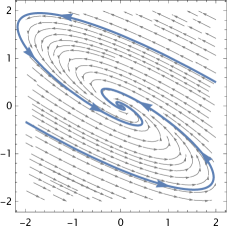
Figure 3: Phase-portrait of (3.2) with $\displaystyle w_{ij}=w_{ij}^{*}+\delta_{ij}$ with $\displaystyle a_{1}=-2$, $\displaystyle a_{2}=1$, $\displaystyle\delta_{ij}=\frac{1}{5}$.

It would be interesting to investigate, however, if higher-order interactions [4] can stabilize the origin. This is, in general, a very complicated problem and we limit ourselves to providing a proof of concept. Suppose one introduces higher-order terms as follows:

$$\begin{split}\dot{x}_{1}&=a_{1}x_{1}+w_{12}(x_{2}-x_{1})-wx_{2}^{3}+w(x_{1}+x_{2})^{3}\\ \dot{x}_{2}&=a_{2}x_{2}+w_{21}(x_{1}-x_{2})+wx_{2}^{3},\end{split}$$ (3.11)

where $\displaystyle w\in\mathbb{R}$. Upon a time-rescaling, one can assume that all parameters are small. To simplify the analysis, but keeping the problem still interesting, let $\displaystyle a_{1}=\alpha$ and $\displaystyle a_{2}=-\alpha$ with $\displaystyle\alpha>0$, hence the uncoupled dynamics are unstable. We emphasize that the origin is still nilpotent for (3.11) with $\displaystyle w_{ij}=w_{ij}^{*}$. Consider the polar blow-up

$$(x,y)=(r\cos(\theta),r\sin(\theta))$$ (3.12)

together with the rescaling of parameters $\displaystyle\alpha=r^{3}A,w=rW$. In these new coordinates, and after division by $\displaystyle r^{3}$, we obtain the vector field

$$\begin{split}r^{\prime}&=rf_{1}(\theta)\\ \theta^{\prime}&=f_{2}(\theta)\end{split}$$ (3.13)

where, having substituted $\displaystyle w_{ij}=w_{ij}^{*}$, we have

$$\begin{split}f_{1}(\theta)&=\frac{1}{8}(4A\cos(2\theta)+W(6\sin(2\theta)+3\sin(4\theta)-\cos(4\theta)+9))\\ f_{2}(\theta)&=\frac{1}{8}(-2(2A+3W)\sin(2\theta)-4A+W\sin(4\theta)+3W\cos(4\theta)-3W).\end{split}$$ (3.14)

It follows that if we let $\displaystyle W=-A$, then (3.13) has eight hyperbolic equilibria for $\displaystyle r=0$ given by

$$\{\theta_{i}\}\approx\{0.431808,1.26918,2.35619,2.54775,3.5734,4.41077,5.49779,5.68935\},\;i=1,\ldots,8,$$ (3.15)

where in particular $\displaystyle(r,\theta)=(0,\theta_{k})$, $\displaystyle k=2,4,6,8$, are stable nodes and the rest are saddles with the $\displaystyle r$-direction stable. This leads to the diagram shown in figure 4.

Remark 11.

Notice that thanks to the higher-order terms, the equilibria of the blown-up system are hyperbolic. That is, one can indeed desingularize a nilpotent equilibrium of a network dynamical system via the blow-up.

Due to hyperbolicity, a qualitatively similar result, as the one stated above, holds for $\displaystyle W\approx-A$. Moreover, since the result does not depend on the rescaling of the parameters, just on their signs, we conclude that the origin of (3.11) is stable for $\displaystyle a_{1}=\alpha$, $\displaystyle a_{2}=-\alpha$ with $\displaystyle\alpha>0$ and $\displaystyle w<0$, see a simulation in figure 4.

Figure 4: (a) Global phase-portrait of (3.13), where all equilibria are hyperbolic. Panels (b) and (c) show a simulation of (3.11) with $\displaystyle a_{1}=1$, $\displaystyle a_{2}=-1$, $\displaystyle w_{ij}=w_{ij}^{*}$, $\displaystyle w=-1/10$ and $\displaystyle w=-2$ respectively.

The main conclusions of the previous analysis are summarized as follows.

Proposition 1.

Consider the 2-node network

$$\begin{split}\dot{x}_{1}&=a_{1}x_{1}+w_{12}(x_{2}-x_{1})-wx_{2}^{3}+w(x_{1}+x_{2})^{3}\\ \dot{x}_{2}&=a_{2}x_{2}+w_{21}(x_{1}-x_{2})+wx_{2}^{3},\end{split}$$ (3.16)

with parameters satisfying (3.3) so that the origin is nilpotent. If $\displaystyle w=0$ then the origin is unstable. On the other hand, if $\displaystyle a_{1}=-a_{2}=\alpha$ with $\displaystyle\alpha>0$ and $\displaystyle w<0$, then the origin is locally asymptotically stable.

The general case (3.1) quickly becomes analytically intractable. For example, it is quite difficult to find closed expressions for the parameters such that the origin is nilpotent. Nevertheless, we conjecture that the dynamics shall be reminiscent of what is shown in figure 2, and that as for the case $\displaystyle N=2$, higher-order interactions may stabilize nilpotent points. A special case that is simple to analyze is considered in the following proposition.

Proposition 2.

Consider

$$\dot{x}_{i}=a_{i}x_{i}+\sum_{j=1}^{N}w_{ij}(x_{j}-x_{i})+h_{i}(x),$$ (3.17)

with $\displaystyle h_{i}(0)=0$, $\displaystyle h_{i}\in\mathcal{O}(|x|^{2})$, and with parameters $\displaystyle a_{i}\in\mathbb{R}$, $\displaystyle a_{i}\neq 0$, and $\displaystyle w_{ij}\in\mathbb{R}$ such that the origin is nilpotent. Suppose that there exists a smooth function $\displaystyle V:\mathbb{R}^{n}\to\mathbb{R}$ such that $\displaystyle h(x)=(h_{1}(x),\ldots,h_{n}(x))=-\nabla V(x)$ and $\displaystyle x=0$ is a (degenerate, since $\displaystyle h_{i}\in\mathcal{O}(|x|^{2})$) local minimum of $\displaystyle V$. Then the origin is locally asymptotically stable.

Proof.

System (3.1) can be rewritten as the gradient system $\displaystyle\dot{x}=-\nabla W$ where $\displaystyle W=(W_{1},\ldots,W_{n})$ with $\displaystyle W_{i}=-(a_{i}-w_{ii})x_{i}^{2}-\sum_{i=1,\,i\neq j}^{n}w_{ij}x_{i}x_{j}+V$. The statement is now straightforward from noticing that the nilpotent assumption guarantees that the origin is a (degenerate) local minimum of $\displaystyle W$. ∎

Remark 12.

Proposition 2 concerns network dynamical systems for which the leading part is nilpotent and the higher-order terms are of gradient form. The proposition roughly tells us that near the nilpotent point, the system behaves as a gradient system, hence the higher-order terms, if chosen appropriately, stabilize the nilpotent origin. Naturally, many network dynamical systems do not admit a gradient structure. In particular, one can check that (3.11) is not of such a gradient form.

3.2 An example of nilpotent internal dynamics

Consider the following system of weakly and diffusely coupled scalar nodes

$$\begin{split}\dot{x}_{i}&=a_{i}x_{i}^{3}(1-x_{i})+\varepsilon\sum_{j=1}^{N}w_{ij}(x_{j}-x_{i}),\end{split}$$ (3.18)

where $\displaystyle a_{i}\neq 0$, $\displaystyle w_{ij}\in\mathbb{R}$, and for simplicity we assume that $\displaystyle x_{i}(0)\in(0,1)$, and that $\displaystyle w_{ii}=0$ for all $\displaystyle i=1,\ldots,N$ (there are no self-couplings). Since for $\displaystyle\varepsilon=0$ the origin is nilpotent, we are going to use the blow-up technique to elucidate the stability of the origin for $\displaystyle\varepsilon$ small.

A node directional blow-up given by

$$(r,r\bar{x}_{1},\ldots,r\bar{x}_{i-1},r\bar{x}_{i+1},\ldots,r\bar{x}_{N},r^{2}\bar{\varepsilon})=(x_{i},x_{1},\ldots,x_{i-1},x_{i+1},\ldots,x_{N},\varepsilon)$$ (3.19)

leads, after desingularization, to

$$\begin{split}r^{\prime}&=r\left(a_{i}+\bar{\varepsilon}\sum_{j=1}^{N}w_{ij}(\bar{x}_{j}-1)-a_{i}r\right)\\ \bar{x}_{k}^{\prime}&=a_{k}\bar{x}_{k}^{3}+\bar{\varepsilon}\sum_{j\neq i}^{N}w_{kj}(\bar{x}_{j}-\bar{x}_{k})+\bar{\varepsilon}w_{ki}(1-\bar{x}_{k})-\bar{x}_{k}\left(a_{i}+\bar{\varepsilon}\sum_{j=1}^{N}w_{ij}(\bar{x}_{j}-1)-a_{i}r\right)-ra_{k}\bar{x}_{k}^{4}\\ \bar{\varepsilon}^{\prime}&=-2\bar{\varepsilon}\left(a_{i}+\bar{\varepsilon}\sum_{j=1}^{N}w_{ij}(\bar{x}_{j}-1)-a_{i}r\right),\end{split}$$ (3.20)

$\displaystyle k=1,\ldots,N$ with $\displaystyle k\neq i$. In this model $\displaystyle x_{i}$ is replaced by $\displaystyle r$, hence one is interested in the stability of $\displaystyle r=0$, which we recall corresponds to the origin via the blow-up transformation.

As is usual in the blow-up analysis, one is interested in the dynamics restricted to the invariant subspaces $\displaystyle\left\{r=\bar{\varepsilon}=0\right\}$, $\displaystyle\left\{\bar{\varepsilon}=0\right\}$ and $\displaystyle\left\{r=0\right\}$ (although in this case, it suffices to take the last two subspaces). For $\displaystyle\bar{\varepsilon}=0$ we have

$$\begin{split}r^{\prime}&=a_{i}r(1-r)\\ \bar{x}_{k}^{\prime}&=-a_{i}\bar{x}_{k}+a_{k}\bar{x}_{k}^{3}+r(a_{i}\bar{x}_{k}-a_{k}\bar{x}_{k}^{4})\\ \bar{\varepsilon}^{\prime}&=0,\end{split}$$ (3.21)

where it is straightforward to see, from the leading order terms, that if $\displaystyle a_{l}<0$ for all $\displaystyle l=1,\ldots,N$ we have that, locally, $\displaystyle(r,\bar{x}_{k})=(0,0)$ is a hyperbolic saddle while $\displaystyle(r,\bar{x}_{k})=(0,\pm\sqrt{a_{i}/a_{k}})$ are hyperbolic sinks, with Jacobians

$$J_{(0,0)}=\begin{bmatrix}a_{i}&0\\ 0&-a_{i}\end{bmatrix}\qquad\textnormal{and}\qquad J_{\left(0,\pm\sqrt{a_{i}/a_{k}}\right)}=\begin{bmatrix}a_{i}&0\\ *&2a_{i}\end{bmatrix}$$ (3.22)

respectively. It will be useful for our arguments below to notice that these stability properties depend only on the $\displaystyle a_{i}$ coefficient.

Since the above equilibria are hyperbolic after the blow-up, one can conclude that for $\displaystyle\bar{\varepsilon}>0$ small, the local stability properties of the equilibria are preserved.

In the $\displaystyle\bar{\varepsilon}$-direction (the rescalling chart) we obtain the desingularized system

$$\begin{split}\dot{\bar{x}}_{i}&=a_{i}\bar{x}_{i}^{3}(1-\bar{x}_{i})+\sum_{j=1}^{N}w_{ij}(\bar{x}_{j}-\bar{x}_{i}),\end{split}$$ (3.23)

The leading order term is now the interaction. Therefore, the origin is not nilpotent anymore, but semi-hyperbolic. It follows that if all the weights $\displaystyle w_{ij}$ are nonnegative, and the digraph is strongly connected, then the subspace $\displaystyle\textnormal{span}\left\{1,\ldots,1\right\}\in\mathbb{R}^{N}$ is locally attracting. The dynamics on such a space are thus given by the scalar equation

$$\bar{x}=a_{i}\bar{x}^{3}(1-\bar{x}),$$ (3.24)

for which the origin is locally asymptotically stable provided that $\displaystyle a_{i}<0$.

From our previous analysis, we have proven the following:

Proposition 3.

If $\displaystyle a_{i}<0$, $\displaystyle w_{ij}\leq 0$ for all $\displaystyle i,j=1,\ldots,N$ and the underlying digraph of (3.18) is strongly connected, then the (nilpotent) origin of (3.18) is locally asymptotically stable for $\displaystyle\varepsilon>0$ sufficiently small.

3.3 A slowly adaptive network

Let us consider an adaptive network of $\displaystyle N$ homogeneous Kuramoto oscillators given by [2]

$$\begin{split}\dot{\phi}_{i}&=\omega-\frac{1}{N}\sum_{j=1}^{N}\kappa_{ij}\sin(\phi_{i}-\phi_{j}+\alpha)\\ \dot{\kappa}_{ij}&=-\varepsilon(\sin(\phi_{i}-\phi_{j}+\beta)+\kappa_{ij}).\end{split}$$ (3.25)

Without loss of generality, one may consider $\displaystyle\omega=0$ by changing to the co-rotating frame $\displaystyle\phi_{i}\mapsto\phi_{i}+\omega t$. Thus, from now on we consider

$$\begin{split}\dot{\phi}_{i}&=-\frac{1}{N}\sum_{j=1}^{N}\kappa_{ij}\sin(\phi_{i}-\phi_{j}+\alpha)\\ \dot{\kappa}_{ij}&=-\varepsilon(\sin(\phi_{i}-\phi_{j}+\beta)+\kappa_{ij}).\end{split}$$ (3.26)

A one-cluster solution is defined as $\displaystyle\phi_{i}(t)=s(t)+a_{i}$ for some constant $\displaystyle a_{i}\in[0,2\pi)$, $\displaystyle i=1\ldots,N$. Depending on the phases $\displaystyle a_{i}$ the aforementioned one-cluster solutions receive different names, see [2, Definition 2.3]. Upon substitution of the one-cluster solution in (3.26) one finds that $\displaystyle\dot{s}=$constant, meaning that one-cluster solutions are, in fact, of the form $\displaystyle\phi_{i}(t)=\Omega t+a_{i}$, with some $\displaystyle\Omega\in\mathbb{R}$. It is well-known that the one-cluster solutions with $\displaystyle\Omega=\Omega^{*}:=\frac{1}{N}\sum_{j}\sin(a_{i}-a_{j}+\alpha)\sin(a_{i}-a_{j}+\beta)$, together with $\displaystyle k_{ij}(t)=-\sin(a_{i}-a_{j}+\beta)$ form a set of relative equilibria of (3.26). In other words, consider the co-rotating coordinates $\displaystyle\psi_{i}=\phi_{i}-(\Omega^{*}t+a_{i})$, and the shifted weights $\displaystyle\sigma_{ij}=\kappa_{ij}+\sin(a_{i}-a_{j}+\beta)$. Then (3.26) is re-written as

$$\begin{split}\dot{\psi}_{i}&=-\Omega^{*}+\frac{1}{N}\sum_{j=1}^{N}\sin(a_{i}-a_{j}+\beta)\sin(\psi_{i}+a_{i}-\psi_{j}-a_{j}+\alpha)\\ &\quad-\frac{1}{N}\sum_{j=1}^{N}\sigma_{ij}\sin(\psi_{i}+a_{i}-\psi_{j}-a_{j}+\alpha)\\ \dot{\sigma}_{ij}&=-\varepsilon(\sin(\psi_{i}+a_{i}-\psi_{j}-a_{j}+\beta)-\sin(a_{i}-a_{j}+\beta)+\sigma_{ij})\end{split}$$ (3.27)

It follows, indeed, that $\displaystyle(\psi_{i}^{*},\sigma_{ij}^{*})=(0,0)$ is an equilibrium of (3.27). It turns out that this equilibrium is non-hyperbolic from a slow-fast perspective. Moreover, for certain parameters, one-cluster solutions can be nilpotent.

Proposition 4.

Consider the layer equation of (3.27). Then the equilibrium point $\displaystyle(\psi_{i}^{*},\sigma_{ij}^{*})=(0,0)$ is non-hyperbolic. In particular, the antipodal solution, which corresponds to $\displaystyle a_{i}\in\left\{0,\pi\right\}$, is nilpotent for $\displaystyle\beta=0$.

Remark 13.

These are not the only nilpotent solutions. In fact, for $\displaystyle\alpha=\beta=0$ all one-cluster solutions in [2, Corollary 4.3] are nilpotent. In this example, however, we only concentrate on the antipodal case.

Proof.

Since we are looking at the layer equation of (3.27), we only need to consider the Jacobian $\displaystyle J=[J_{ij}]_{i,j=1,\ldots,N}$ where $\displaystyle J_{ij}=\frac{\partial\dot{\psi}_{i}}{\partial\psi_{j}}\Big{|}_{\psi_{i}=\psi_{j}=\sigma_{ij}=0}$. So, we have

$$\begin{split}J_{ii}&=\frac{1}{N}\sum_{j=1}^{N}\sin(a_{i}-a_{j}+\beta)\cos(a_{i}-a_{j}+\alpha)\\ J_{ij}&=\frac{1}{N}\sin(a_{i}-a_{j}+\beta)\cos(a_{i}-a_{j}+\alpha).\end{split}$$ (3.28)

Since $\displaystyle J_{ii}+\sum_{j\neq i}^{N}J_{ij}=0$, it follows that $\displaystyle\ker J$ is non-trivial (this is reminiscent, of course, of Laplacian matrices), showing that the equilibrium point $\displaystyle(\psi_{i}^{*},\sigma_{ij}^{*})=(0,0)$ is non-hyperbolic. Finally, if $\displaystyle\beta=0$ and $\displaystyle a_{i}\in\left\{0,\pi\right\}$ we have that $\displaystyle J=0$, i.e., the equilibrium point $\displaystyle(\psi_{i}^{*},\sigma_{ij}^{*})=(0,0)$ is nilpotent. ∎

The question one would now like to answer is: what is the stability of the anti-podal solutions for $\displaystyle\varepsilon,\,\beta$ small? To answer this question we are going to use the blow-up technique. We remark that the blow-up technique is a local tool, hence, it is in principle applied to polynomial vector fields. Here we shall simply expand (3.27) for $\displaystyle(\psi_{i},\sigma_{ij})$ close to the origin. Let $\displaystyle a_{i}\in\left\{0,\pi\right\}$. Up to a constant shift above, we can assume without loss of generality that $\displaystyle a_{i}=0$ for all $\displaystyle i=1,\ldots,N$. Then (3.27) reads as

$$\begin{split}\dot{\psi}_{i}&=-\Omega^{*}+\frac{1}{N}\sum_{j=1}^{N}\sin\beta\sin(\psi_{i}-\psi_{j}+\alpha)-\frac{1}{N}\sum_{j=1}^{N}\sigma_{ij}\sin(\psi_{i}-\psi_{j}+\alpha)\\ \dot{\sigma}_{ij}&=-\varepsilon(\sin(\psi_{i}-\psi_{j}+\beta)-\sin\beta+\sigma_{ij}).\end{split}$$ (3.29)

Expanding $\displaystyle\sin(\psi_{i}-\psi_{j}+\rho)$ for $\displaystyle\psi_{i}\approx\psi_{j}$, i.e. ($\displaystyle\sin(\psi_{i}-\psi_{j}+\rho)=\sin\rho+\cos\rho(\psi_{i}-\psi_{j})+\cdots$), with $\displaystyle\rho=\alpha,\beta$, and accounting for the fact that in this setup we have $\displaystyle-\Omega^{*}+\sin\alpha\sin\beta=0$, we get

$$\begin{split}\dot{\psi}_{i}&=\frac{1}{N}\sum_{j=1}^{N}\left[\sin\beta\cos\alpha(\psi_{i}-\psi_{j})-\sigma_{ij}(\sin\alpha+\cos\alpha(\psi_{i}-\psi_{j})\right]+\cdots\\ \dot{\sigma}_{ij}&=-\varepsilon\left(\cos\beta(\psi_{i}-\psi_{j})+\sigma_{ij}+\cdots\right),\end{split}$$ (3.30)

where the $\displaystyle\cdots$ indicate higher-order terms. Naturally, the origin $\displaystyle(\psi_{i},\sigma_{ij})=(0,0)$ is (still) nilpotent for $\displaystyle\varepsilon=\beta=0$, but now it is straightforward to notice that $\displaystyle\alpha=\pm\frac{\pi}{2}$ also induces that the origin is nilpotent (this case is not further discussed in this example). For the rest of this example, we only consider the leading part of (3.30).

Let us propose the $\displaystyle\beta$-directional blow-up (in the rescaling chart) given by

$$\psi_{i}=ru_{i},\quad\sigma_{ij}=rs_{ij},\quad\alpha=rA,\quad\beta=\pm r,\quad\varepsilon=r.$$ (3.31)

This leads to the desingularized vector field (where we take only the leading order terms of the Taylor expansion of the trigonometric functions)

$$\begin{split}\dot{r}&=0\\ \dot{u}_{i}&=\frac{1}{N}\sum_{j=1}^{N}\pm(u_{i}-u_{j})-s_{ij}(A+(u_{i}-u_{j}))\\ \dot{s}_{ij}&=-((u_{i}-u_{j})+s_{ij}).\end{split}$$ (3.32)

Now, the following conclusions on the local stability of the line of equilibria $\displaystyle u_{i}=u_{j},\,s_{ij}=0$, which we denote by $\displaystyle\gamma$, are straightforward: a) if $\displaystyle\beta>0$, corresponding to the plus sign in (3.32), then $\displaystyle\gamma$ cannot be stable; b) if $\displaystyle\beta<0$, corresponding to the negative sign in (3.32), then $\displaystyle\gamma$ is locally stable for $\displaystyle A<1$ and unstable for $\displaystyle A>1$. From this analysis, and recalling the blow-up map (3.31), the following statement is proven (compare with [2, figure 4.2 (b)]):

Proposition 5.

The antipodal solutions of (3.26) are locally asymptotically stable for $\displaystyle\beta<-\alpha$ and $\displaystyle\varepsilon>0$ sufficiently small.

4 Conclusions and Discussion

We have studied the problem of structure preservation under the blow-up transformation of network dynamical systems, including adaptive ones. This transformation is a useful tool to rigorously analyze the dynamics of differential equations close to nilpotent equilibria. The essential philosophy of the method is to transform a singular problem into a regular one.

The main conclusion from our analysis is that, indeed, the blow-up transformation preserves the network structure. This means that the local vector fields obtained after a directional blow-up can still be interpreted as a network dynamical system. The precise interpretation turns out to depend on the direction of blow-up and the model at hand. Moreover, via a series of examples, we have shown that (as in the classical low-dimensional setting) the blow-up helps to desingularize nilpotent singularities.

Besides structure preservation, we have noticed that the blow-up induces parameters to become dynamic. Nevertheless, such dynamics seem to occur at higher-orders, which could yield another natural way to uncover higher-interactions in networks. In the particular case of edge-directional blow-up, including the case of adaptive networks, the main message is that singular networks with static topology are to be regularized as network dynamical systems with co-evolving edges; hence, this provides a route to potentially uncover adaptive network dynamics.

Several open problems stem from the analysis presented here, from which we highlight the following:

1. The problem of desingularization has been addressed here only in the examples. It would be interesting to relate the network topology and the nature of internal dynamics, interaction, and possible adaptation, to better describe the desingularization procedure via blow-up. In particular, one may want to study classes of networked systems where the corresponding vector field is quasi-homogeneous.

2. For high-dimensional problems, it may become unrealistic to blow-up in all possible directions. This raises new directions for improving and better adapting the blow-up method for networks: a) one may want to blow-up in several directions simultaneously, b) one may want to devise techniques that distinguish between regular and singular directions, or c) one may want to develop symbolic computational tools that automatically provide the local vector fields in the relevant charts where the dynamics have been desingularized.

3. Choosing the blow-up weights is, even for low dimensions, quite challenging. In the context of networks, it is not unfeasible to expect that the topology of the network induces, or forces, some patterns in the blow-up weights. For example, the analysis carried out in section 2 suggests that, due to the network structure, all nodes are to be blown up with the same weight, provided that the linear part is not identically zero. In this regard, it is known that the quasi-homogeneous blow-up for planar systems can be related to a Newton polyhedron, see [1]. In higher dimensions, the quasihomogeneous blow-up should naturally be related to a polytope. It would be interesting to see if there is a relation between the blow-up polytope and the topology of the network to be desingularized.

4. A way to describe the dynamics of large networks is via mean field limits, which essentially provides a low-dimensional averaged description (e.g. via a PDE, but in certain cases even a low-dimensional system of ODEs) of the network. It would be interesting to investigate if a desingularization of a mean-field limit corresponds, in any way, to the desingularization of the corresponding large, but finite, network.

References

- Álvarez et al. [2011] María Jesús Álvarez, Antoni Ferragut, and Xavier Jarque. A survey on the blow up technique. International Journal of Bifurcation and Chaos, 21(11):3103–3118, 2011.
- Berner et al. [2019] Rico Berner, Eckehard Schöll, and Serhiy Yanchuk. Multiclusters in Networks of Adaptively Coupled Phase Oscillators. SIAM Journal on Applied Dynamical Systems, 18(4):2227–2266, 2019.
- Berner et al. [2023] Rico Berner, Thilo Gross, Christian Kuehn, Jürgen Kurths, and Serhiy Yanchuk. Adaptive dynamical networks. arXiv preprint arXiv:2304.05652, 2023.
- Bick et al. [2023] Christian Bick, Elizabeth Gross, Heather A Harrington, and Michael T Schaub. What are higher-order networks? SIAM Review, 65(3):686–731, 2023.
- Bonetto and Jardón-Kojakhmetov [2022] Riccardo Bonetto and Hildeberto Jardón-Kojakhmetov. Nonlinear Laplacian Dynamics: Symmetries, Perturbations, and Consensus. arXiv preprint arXiv:2206.04442, 2022.
- Dumortier [1993] Freddy Dumortier. Techniques in the theory of local bifurcations: Blow-up, normal forms, nilpotent bifurcations, singular perturbations. Bifurcations and periodic orbits of vector fields, pages 19–73, 1993.
- Dumortier and Roussarie [1996] Freddy Dumortier and Robert H Roussarie. Canard cycles and center manifolds, volume 577. American Mathematical Soc., 1996.
- Elmhirst and Golubitsky [2006] Toby Elmhirst and Martin Golubitsky. Nilpotent Hopf bifurcations in coupled cell systems. SIAM Journal on Applied Dynamical Systems, 5(2):205–251, 2006.
- Engel and Kuehn [2020] Maximilian Engel and Christian Kuehn. Blow-up analysis of fast-slow PDEs with loss of hyperbolicity. arXiv preprint arXiv:2007.09973, 2020.
- Engel et al. [2022] Maximilian Engel, Felix Hummel, Christian Kuehn, Nikola Popović, Mariya Ptashnyk, and Thomas Zacharis. Geometric analysis of fast-slow PDEs with fold singularities. arXiv preprint arXiv:2207.06134, 2022.
- Gkogkas and Kuehn [2022] Marios Antonios Gkogkas and Christian Kuehn. Graphop mean-field limits for kuramoto-type models. SIAM Journal on Applied Dynamical Systems, 21(1):248–283, 2022.
- Golubitsky and Lauterbach [2009] Martin Golubitsky and Reiner Lauterbach. Bifurcations from synchrony in homogeneous networks: linear theory. SIAM Journal on Applied Dynamical Systems, 8(1):40–75, 2009.
- Golubitsky and Stewart [2006] Martin Golubitsky and Ian Stewart. Nonlinear dynamics of networks: the groupoid formalism. Bulletin of the american mathematical society, 43(3):305–364, 2006.
- Hayes et al. [2016] Michael G Hayes, Tasso J Kaper, Peter Szmolyan, and Martin Wechselberger. Geometric desingularization of degenerate singularities in the presence of fast rotation: A new proof of known results for slow passage through hopf bifurcations. Indagationes Mathematicae, 27(5):1184–1203, 2016.
- Hummel et al. [2022] Felix Hummel, Samuel Jelbart, and Christian Kuehn. Geometric blow-up of a dynamic Turing instability in the Swift-Hohenberg equation. arXiv preprint arXiv:2207.03967, 2022.
- Jardón-Kojakhmetov and Kuehn [2020] Hildeberto Jardón-Kojakhmetov and Christian Kuehn. On fast–slow consensus networks with a dynamic weight. Journal of Nonlinear Science, 30(6):2737–2786, 2020.
- Jardón-Kojakhmetov and Kuehn [2021] Hildeberto Jardón-Kojakhmetov and Christian Kuehn. A survey on the blow-up method for fast-slow systems, volume 775, pages 115–160. AMS Press, 2021. 10.1090/conm/775/15591.
- Jardón-Kojakhmetov et al. [2023] Hildeberto Jardón-Kojakhmetov, Christian Kuehn, and Iacopo P. Longo. Persistent synchronization of heterogeneous networks with time-dependent linear diffusive coupling. arXiv preprint arXiv:2305.05747, 2023.
- Jelbart and Kuehn [2023] Samuel Jelbart and Christian Kuehn. A Formal Geometric Blow-up Method for Pattern Forming Systems. arXiv preprint arXiv:2302.06343, 2023.
- Krupa and Szmolyan [2001] Martin Krupa and Peter Szmolyan. Extending geometric singular perturbation theory to nonhyperbolic points—fold and canard points in two dimensions. SIAM journal on mathematical analysis, 33(2):286–314, 2001.
- Kuehn [2015] Christian Kuehn. Multiple time scale dynamics, volume 191. Springer, 2015.
- Kuehn [2016] Christian Kuehn. A remark on geometric desingularization of a non-hyperbolic point using hyperbolic space. In Journal of Physics: Conference Series, volume 727, page 012008. IOP Publishing, 2016.
- Lancellotti [2005] Carlo Lancellotti. On the Vlasov limit for systems of nonlinearly coupled oscillators without noise. Transport theory and statistical physics, 34(7):523–535, 2005.
- Maria da Conceiçao and Golubitsky [2006] A Leite Maria da Conceiçao and Martin Golubitsky. Homogeneous three-cell networks. Nonlinearity, 19(10):2313, 2006.
- Menini and Tornambè [2010] Laura Menini and Antonio Tornambè. Stability analysis of planar systems with nilpotent (non-zero) linear part. Automatica, 46(3):537–542, 2010.
- Newman [2018] Mark Newman. Networks. Oxford university press, 2018.
- Nijholt et al. [2023] Eddie Nijholt, Tiago Pereira, Fernando C Queiroz, and Dmitry Turaev. Chaotic Behavior in Diffusively Coupled Systems. Communications in Mathematical Physics, pages 1–42, 2023.
- Panazzolo [2002] Daniel Panazzolo. Desingularization of nilpotent singularities in families of planar vector fields. American Mathematical Soc., 2002.
- Panazzolo [2006] Daniel Panazzolo. Resolution of singularities of real-analytic vector fields in dimension three. 2006.
- Porter and Gleeson [2016] Mason A Porter and James P Gleeson. Dynamical systems on networks. Frontiers in Applied Dynamical Systems: Reviews and Tutorials, 4, 2016.
- Sawicki et al. [2023] Jakub Sawicki, Rico Berner, Sarah AM Loos, Mehrnaz Anvari, Rolf Bader, Wolfram Barfuss, Nicola Botta, Nuria Brede, Igor Franović, Daniel J Gauthier, et al. Perspectives on adaptive dynamical systems. arXiv preprint arXiv:2303.01459, 2023.
- Schwemmer and Lewis [2012] Michael A Schwemmer and Timothy J Lewis. The theory of weakly coupled oscillators. Phase response curves in neuroscience: theory, experiment, and analysis, pages 3–31, 2012.
- Sclosa [2021] Davide Sclosa. Completely Degenerate Equilibria of the Kuramoto Model on Networks. arXiv preprint arXiv:2112.12034, 2021.
- Strogatz [2001] Steven H Strogatz. Exploring complex networks. nature, 410(6825):268–276, 2001.
- Takens [1974] Floris Takens. Singularities of vector fields. Publications Mathématiques de l’IHÉS, 43:47–100, 1974.
- Wechselberger [2020] Martin Wechselberger. Geometric singular perturbation theory beyond the standard form, volume 6. Springer, 2020.