Performance of a PEM fuel cell cathode catalyst layer under oscillating potential and oxygen supply

Abstract

A model for impedance of a PEM fuel cell cathode catalyst layer under simultaneous application of potential and oxygen concentration perturbations is developed and solved. The resulting expression demonstrates dramatic lowering of the layer impedance under increase in the amplitude of the oxygen concentration perturbation. In–phase oscillations of the overpotential and oxygen concentration lead to formation of a fully transparent to oxygen sub–layer. This sub–layer works as an ideal non polarizable electrode, which strongly reduces the system impedance.

I Introduction

Electrochemical impedance spectroscopy (EIS) has proven to be a unique non–destructive and non–invasive tool for fuel cells characterization [1]. In its classic variant, EIS implies application of a small–amplitude harmonic perturbation of the cell current or potential and measuring the response of the cell potential or current, respectively. In recent years, there has been interest in alternative techniques based on application of pressure (Engebretsen et al. [2], Shirsath et al. [3], Schiffer et al. [4], Zhang et al. [5]) or oxygen concentration (Sorrentino et al. [6, 7, 8]) perturbation to the cell and measuring the response of electric variable (potential or current), keeping the second electric variable constant.

Application of pressure oscillations at the cathode channel inlet or outlet inevitably leads to flow velocity oscillations (FVO). Kim et al.  [9] and Hwang et al.  [10] reported experiments showing dramatic improvement of PEM fuel cell performance under applied FVO. The effect of FVO on the cell performance was more pronounced with lower static flow rates and with increasing the FVO amplitude [9]. In [9, 10], the effect has been attributed to improvement of diffusive oxygen transport through the cell due to FVO. Kulikovsky [11, 12] developed a simplified analytical model for impedance of the cell subjected to simultaneous oscillations of potential and air flow velocity. The model have shown reduction of the cell static resistivity upon increase of the FVO amplitude. Yet, however, due to system complexity, the mechanism of cell performance improvement is not clear.

Below, a much simpler system (PEM fuel cell cathode catalyst layer) subjected to oscillating in–phase potential and oxygen supply is considered. Analytical model for the CCL impedance under these conditions is solved. The result demonstrates the effect of impedance reduction due to oscillating oxygen supply. In–phase oxygen concentration and overpotential oscillations make part of the catalyst layer at the cathode catalyst layer (CCL)/gas diffusion layer (GDL) interface fully transparent to oxygen, which leads to dramatic decrease of the system impedance.

II Model

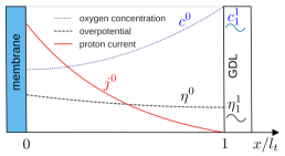
Figure 1: Schematic of the cathode catalyst layer and typical shapes of the oxygen concentration, proton current and overpotential through the layer. In–phase harmonic perturbations of the overpotential $\eta_{1}^{1}$ and oxygen concentration $c_{1}^{1}$ are applied at the CCL/GDL interface.

Consider a problem for impedance of the cathode catalyst layer (CCL) under oscillating potential and oxygen supply (Figure 1). For simplicity, we will assume that the proton transport is fast. The model is based on two equations: the proton charge conservation

$$C_{dl}\dfrac{\partial{\eta}}{\partial{t}}+\dfrac{\partial{j}}{\partial{x}}=-i_{*}\left(\dfrac{c}{c_{ref}}\right)\exp\left(\dfrac{\eta}{b}\right)$$ (1)

and the oxygen mass transport equation

$$\dfrac{\partial{c}}{\partial{t}}-D_{ox}\dfrac{\partial^{2}{c}}{\partial{x}^{2}}=-\dfrac{i_{*}}{4F}\left(\dfrac{c}{c_{ref}}\right)\exp\left(\dfrac{\eta}{b}\right).$$ (2)

Here, $x$ is the distance through the CCL, $C_{dl}$ is the double layer capacitance, $\eta$ is the positive by convention ORR overpotential, $t$ is time, $j$ is the local proton current density, $x$ is the coordinate through the CCL, $i_{*}$ is the ORR volumetric exchange current density, $c_{ref}$ is the reference oxygen concentration, and $b$ is the ORR Tafel slope. Introducing dimensionless variables

$$\tilde{x}=\dfrac{x}{l_{t}},\quad\tilde{t}=\dfrac{ti_{*}}{C_{dl}b},\quad\tilde{c}=\dfrac{c}{c_{ref}},\quad\tilde{\eta}=\dfrac{\eta}{b},\quad\tilde{j}=\dfrac{j}{i_{*}l_{t}},\\ \tilde{D}_{ox}=\dfrac{4FD_{ox}c_{ref}}{i_{*}l_{t}^{2}},\quad\tilde{Z}=\dfrac{Zi_{*}l_{t}}{b},\quad\tilde{\omega}=\dfrac{\omega C_{dl}b}{i_{*}},$$ (3)

where $\tilde{\omega}$ is the angular frequency of applied AC signal, $\tilde{Z}$ is the CCL impedance, Eqs.(1), (2) take the form

$$\dfrac{\partial{\tilde{\eta}}}{\partial{\tilde{t}}}+\dfrac{\partial{\tilde{j}}}{\partial{\tilde{x}}}=-\tilde{c}\exp\tilde{\eta}$$ (4)

$$\mu^{2}\dfrac{\partial{\tilde{c}}}{\partial{\tilde{t}}}-\tilde{D}_{ox}\dfrac{\partial^{2}{\tilde{c}}}{\partial{\tilde{x}}^{2}}=-\tilde{c}\exp\tilde{\eta},$$ (5)

where $\mu$ is the constant parameter

$$\mu=\sqrt{\dfrac{4Fc_{ref}}{C_{dl}b}}.$$ (6)

Substituting Fourier–transforms of the form

$$\begin{split}&\tilde{\eta}(\tilde{t})=\tilde{\eta}^{0}+\tilde{\eta}_{1}^{1}(\tilde{\omega})\exp({\rm i}\tilde{\omega}\tilde{t}),\quad|\tilde{\eta}_{1}^{1}|\ll\tilde{\eta}^{0}\\ &\tilde{j}(\tilde{x},\tilde{t})=\tilde{j}^{0}(\tilde{x})+\tilde{j}^{1}(\tilde{x},\tilde{\omega})\exp({\rm i}\tilde{\omega}\tilde{t}),\quad|\tilde{j}^{1}|\ll\tilde{j}^{0}\\ &\tilde{c}(\tilde{x},\tilde{t})=\tilde{c}^{0}(\tilde{x})+\tilde{c}^{1}(\tilde{x},\tilde{\omega})\exp({\rm i}\tilde{\omega}\tilde{t}),\quad|\tilde{c}^{1}|\ll\tilde{c}^{0},\end{split}$$ (7)

into Eqs.(4), (5), neglecting terms with the perturbation products and subtracting the respective static equations, we get a system of equations relating the perturbation amplitudes $\tilde{\eta}_{1}^{1}(\tilde{\omega})$, $\tilde{j}^{1}(\tilde{x},\tilde{\omega})$ and $\tilde{c}^{1}(\tilde{x},\tilde{\omega})$ [13]:

$$\dfrac{\partial{\tilde{j}^{1}}}{\partial{\tilde{x}}}=-\exp(\tilde{\eta}^{0})\left(\tilde{c}^{1}+\tilde{c}_{1}^{0}\tilde{\eta}_{1}^{1}\right)-{\rm i}\tilde{\omega}\tilde{\eta}_{1}^{1},\quad\tilde{j}^{1}(1)=0$$ (8)

$$\tilde{D}_{ox}\dfrac{\partial^{2}{\tilde{c}^{1}}}{\partial{\tilde{x}}^{2}}=\exp(\tilde{\eta}^{0})\left(\tilde{c}^{1}+\tilde{c}_{1}^{0}\tilde{\eta}_{1}^{1}\right)+{\rm i}\mu^{2}\tilde{\omega}\tilde{c}^{1},\\ \left.\dfrac{\partial{\tilde{c}^{1}}}{\partial{\tilde{x}}}\right|_{\tilde{x}=0}=0,\quad\tilde{c}^{1}(1)=k\tilde{\eta}_{1}^{1}$$ (9)

where the superscripts 0 and 1 mark the static variables and the small perturbation amplitudes, respectively, $\tilde{c}_{1}^{0}$ is the static oxygen concentration at the CCL/GDL interface, $k\geq 0$ is the constant model parameter, $\tilde{\eta}_{1}^{1}$ is the amplitude of applied potential perturbation.

The boundary condition for Eq.(8) means zero proton current at the CCL/GDL interface. The left boundary condition for Eq.(9) expresses zero oxygen flux through the membrane. The feature of this problem is the right boundary condition for Eq.(9), meaning external control of oxygen concentration perturbation $\tilde{c}^{1}$ at the CCL/GDL interface: $\tilde{c}^{1}(1)$ varies in–phase with the overpotential perturbation $\tilde{\eta}_{1}^{1}$. Note that the perturbations of applied cell potential and overpotential have different signs, assuming that the electron conductivity of the cell components is much larger than the CCVL proton conductivity.

Due to fast proton transport, $\tilde{\eta}_{1}^{1}$ is nearly independent of $\tilde{x}$. For simplicity we will also assume that the variation of static oxygen concentration along $\tilde{x}$ is also small and we set $\tilde{c}^{0}\simeq\tilde{c}_{1}^{0}$. Introducing electric $Y$ and concentration $G$ admittances

$$Y=\dfrac{\tilde{j}^{1}}{\tilde{\eta}_{1}^{1}},\quad G=\dfrac{\tilde{c}^{1}}{\tilde{\eta}_{1}^{1}}$$ (10)

and taking into account the static polarization curve

$$\tilde{j}_{0}=\tilde{c}_{1}^{0}\exp\tilde{\eta}^{0}$$ (11)

we can rewrite the system (8), (9) in terms of $Y$ and $G$:

$$\dfrac{\partial{Y}}{\partial{\tilde{x}}}=-\dfrac{\tilde{j}_{0}}{\tilde{c}_{1}^{0}}\left(G+\tilde{c}_{1}^{0}\right)-{\rm i}\tilde{\omega},\quad Y(1)=0$$ (12)

$$\tilde{D}_{ox}\dfrac{\partial^{2}{G}}{\partial{\tilde{x}}^{2}}=\dfrac{\tilde{j}_{0}}{\tilde{c}_{1}^{0}}\left(G+\tilde{c}_{1}^{0}\right)+{\rm i}\mu^{2}\tilde{\omega}G,\\ \left.\dfrac{\partial{G}}{\partial{\tilde{x}}}\right|_{\tilde{x}=0}=0,\quad G(1)=k.$$ (13)

Eq.(13) can be directly solved:

$$G(\tilde{x})=\dfrac{\tilde{j}_{0}}{\psi^{2}}\left(\dfrac{\cosh(\psi\tilde{x})}{\cosh(\psi)}-1\right)+\dfrac{k\cosh(\psi\tilde{x})}{\cosh(\psi)},\\ \psi\equiv\sqrt{\dfrac{\tilde{j}_{0}}{\tilde{c}_{1}^{0}}+{\rm i}\mu^{2}\tilde{\omega}}.$$ (14)

Using this solution and solving Eq.(12), for the CCL impedance $\tilde{Z}=1/Y|_{\tilde{x}=0}$ we get

$$\tilde{Z}=\dfrac{\tilde{Z}_{RC}}{\left(\tilde{j}_{0}/\tilde{c}_{1}^{0}\right)\left(k\tilde{Z}_{RC}+\tilde{j}_{0}\right)\tilde{Z}_{W}+\left(\tilde{j}_{0}\mu^{2}+\tilde{Z}_{RC}\right){\rm i}\tilde{\omega}},$$ (15)

where $\tilde{Z}_{RC}$ is the parallel $RC$–circuit impedance, and $\tilde{Z}_{W}$ is the Warburg–like impedance:

$$\tilde{Z}_{RC}=\dfrac{\tilde{j}_{0}}{\tilde{c}_{1}^{0}}+{\rm i}\mu^{2}\tilde{\omega},\quad\tilde{Z}_{W}=\dfrac{\tanh\left(\sqrt{\tilde{Z}_{RC}/\tilde{D}_{ox}}\right)}{\sqrt{\tilde{Z}_{RC}/\tilde{D}_{ox}}}$$ (16)

CCL impedance $Z$, Eq.(15), for the current density of 100 mA cm^-2 and the indicated values of parameter $k$ is shown in Figure 2. The other parameters are listed in Table 1. Note that to emphasize the effect, the CCL oxygen diffusivity is taken to be very low, $D_{ox}=10^{-5}$ cm² s^-1.

The Nyquist spectrum corresponding to $k=0$ (no concentration perturbation at the CCL/GDL interface) consists of two partly overlapping arcs, of which the left one is due to charge transfer and the right one is due to oxygen transport (Figure 2a). In Figure 2b, the left peak of $-\operatorname{Im}\left(Z\right)$ (red curve) corresponds to oxygen transport and the right shoulder is due to faradaic reaction.

The perturbation of oxygen concentration at the CCL/GDL interface dramatically changes the Nyquist spectra. With the growth of $k$, the arc due to oxygen transport strongly decreases (Figure 2). Calculation of Eq.(15) limit as $\tilde{\omega}\to 0$ gives the CCL static resistivity

$$\tilde{R}=\dfrac{\phi\coth(\phi)}{\tilde{j}_{0}\left(1+k/\tilde{c}_{1}^{0}\right)},\quad\phi\equiv\sqrt{\dfrac{\tilde{j}_{0}}{\tilde{c}_{1}^{0}\tilde{D}_{ox}}}$$ (17)

which decreases as $k$ increases (Figure 2a).

Figure 3a shows what happens to the $\tilde{x}$–shape of the phase shift between the oxygen concentration $\tilde{c}^{1}$ and overpotential $\tilde{\eta}_{1}^{1}$ (the phase angle of the function $G(\tilde{x})=\tilde{c}^{1}/\tilde{\eta}_{1}^{1}$) as $k$ increases. At $k=0$, there is a large phase shift between $\tilde{c}_{1}$ and $\tilde{\eta}_{1}^{1}$, excluding a single point at $\tilde{x}=1$, where $\tilde{c}^{1}=0$. With $k=0.5$, a finite–thickness domain where $\tilde{c}^{1}$ and $\tilde{\eta}_{1}^{1}$ oscillate almost in–phase forms, and with $k=0.95$ this domain of zero phase shift increases (Figure 3). Zero phase angle between $\tilde{\eta}_{1}^{1}$ and $\tilde{c}^{1}$ means no oxygen transport losses in this domain.

Figure 3b shows the modulus of the right side of Eq.(12), which is the modulus of the ORR rate perturbation. As can be seen, in the domain transparent for oxygen, the ORR rate strongly increases. Thus, with $k>0$, a relatively thin sub–layer at the CCL/GDL interface forms, which works as an ideal non polarizable catalyst layer with fast oxygen transport and large ORR rate. The concerted action of both effects leads to dramatic lowering of the CCL transport impedance.

Further increase in $k$ changes the sign of the phase angle at the membrane interface, meaning formation of inductive loop in the Nyquist spectrum. In this state, the static resistivity drops below the charge–transfer value under constant oxygen supply $R_{ct}=b/j$; this regime deserves special consideration and it is not discussed here. The limiting value $k_{\lim}$ at which $\tilde{R}=\tilde{R}_{ct}=1/\tilde{j}_{0}$ is

$$k_{\lim}=\tilde{c}_{1}^{0}\bigl{(}\phi\coth(\phi)-1\bigr{)}$$ (18)

The states with $k>k_{\lim}$ could be unstable, which needs further studies.

Tafel slope $b$, V	0.03
Double layer capacitance $C_{dl}$, F cm-3	20
Exchange current density $i_{*}$, A cm-3	$10^{-3}$
Oxygen diffusion coefficient
in the CCL, $D_{ox}$, cm2 s-1	$1\cdot 10^{-5}$
Catalyst layer thickness $l_{t}$, cm	$10\cdot 10^{-4}$
Cell temperature $T$, K	273 + 80
Cathode pressure, bar	1.5
Cathode relative humidity, %	50
Cell current density $j_{0}$, A cm-2	$0.1$

Table 1: The cell parameters used in calculations. Parameter $D_{ox}$ is taken to be small to emphasize the effect of oxygen transport in the CCL.

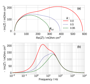
Figure 2: (a) Nyquist spectra of the CCL, Eq.(15), for the indicated values of parameter $k$. The other parameters are listed in Table 1. The point $R_{ct}$ indicates the static charge–transfer resistivity $b/j_{0}$. (b) The frequency dependence of the impedances in (a).

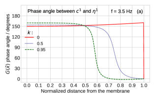
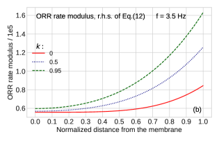
Figure 3: (a) The phase angle of $G=\tilde{c}^{1}/\tilde{\eta}_{1}^{1}$ (between oxygen concentration and overpotential) vs distance $\tilde{x}$ through the CCL. The frequency of 3.5 Hz corresponds to position of the transport peak in Figure 2b. (b) The modulus of the right side of Eq.(12), which is the transient ORR rate.

From practical perspective, in a real fuel cell it is not feasible to directly perturb the oxygen concentration at the CCL/GDL interface in–phase with the overpotential perturbation. However, the experiments of Kim et al.  [9] and Hwang et al.  [10] suggest that the effect could be achieved by perturbing air flow velocity in the channel. Such a perturbation could cause in–phase oscillations of the oxygen concentration and overpotential, which greatly improves the transient cell performance.

Nomenclature

$\tilde{}$	Marks dimensionless variables
$b$	ORR Tafel slope, V
$C_{dl}$	Double layer volumetric capacitance, F cm-3
$c$	Oxygen molar concentration, mol cm-3
$c_{ref}$	Reference oxygen concentration, mol cm-3
$D_{ox}$	Oxygen diffusion coefficient in the CCL, cm2 s-1
$F$	Faraday constant, C mol-1
$f$	Frequency, Hz
$G$	Dimensionless concentration admittance, Eq.(10)
$j$	Local proton current density, A cm-2
${\rm i}$	Imaginary unit
$i_{*}$	ORR volumetric exchange current density, A cm-3
$k$	Concentration amplitude factor, Eq.(9)
$l_{t}$	Catalyst layer thickness, cm
$R$	Static resistivity, $\Omega$ cm2
$t$	Time, s
$x$	Coordinate through the cell, cm
$Y$	Dimensionless electric admittance, Eq.(10)
$Z$	Impedance, $\Omega$ cm2

Subscripts:

$RC$	parallel $RC$–circuit impedance
$W$	Warburg finite–length impedance
$0$	membrane/CCL interface
$1$	CCL/GDL interface

Superscripts:

$0$	Steady–state value
$1$	Small perturbation amplitude

Greek:

$\eta$	ORR overpotential, positive by convention, V
$\eta_{1}^{1}$	Amplitude of applied overpotential perturbation, V
$\mu$	Dimensionless parameter, Eq.(6)
$\phi$	Dimensionless parameter, Eq.(17)
$\psi$	Dimensionless parameter, Eq.(14)
$\omega$	Angular frequency of the AC signal, s-1

References

- Lasia [2014] A. Lasia. Electrochemical Impedance Spectroscopy and its Applications. Springer, New York, 2014.
- Engebretsen et al. [2017] E. Engebretsen, T. J. Mason, P. R. Shearing, G. Hinds, and D. J. L. Brett. Electrochemical pressure impedance spectroscopy applied to the study of polymer electrolyte fuel cells. Electrochem. Comm., 75:60–63, 2017. doi: 10.1016/j.elecom.2016.12.014.
- Shirsath et al. [2020] A. V. Shirsath, S. Rael, C. Bonnet, L. Schiffer, W. Bessler, and F. Lapicque. Electrochemical pressure impedance spectroscopy for investigation of mass transfer in polymer electrolyte membrane fuel cells. Current Opinion in Electrochem., 20:82–87, 2020. doi: 10.1016/j.coelec.2020.04.017.
- Schiffer et al. [2021] L. Schiffer, A. V. Shirsath, S. Raël, F. Lapicque, and W. G. Bessler. Electrochemical pressure impedance spectroscopy for polymer electrolyte membrane fuel cells: A combined modeling and experimental analysis. J. Electrochem. Soc., 169:034503, 2021. doi: 10.1149/1945-7111/ac55cd.
- Zhang et al. [2022] Q. Zhang, H. Homayouni, B. D. Gates, M. Eikerling, and A. M. Niroumand. Electrochemical pressure impedance spectroscopy for polymer electrolyte fuel cells via back-pressure control. J. Electrochem. Soc., 169:044510, 2022. doi: 10.1149/1945-7111/ac6326.
- Sorrentino et al. [2017] A. Sorrentino, T. Vidakovic-Koch, R. Hanke-Rauschenbach, and K. Sundmacher. Concentration–alternating frequency response: A new method for studying polymer electrolyte membrane fuel cell dynamics. Electrochim. Acta, 243:53–64, 2017. doi: 10.1016/j.electacta.2017.04.150.
- Sorrentino et al. [2019] A. Sorrentino, T. Vidakovic-Koch, and K. Sundmacher. Studying mass transport dynamics in polymer electrolyte membrane fuel cells using concentration–alternating frequency response analysis. J. Power Sources, 412:331–335, 2019. doi: 10.1016/j.jpowsour.2018.11.065.
- Sorrentino et al. [2020] A. Sorrentino, K. Sundmacher, and T. Vidakovic-Koch. Polymer electrolyte fuel cell degradation mechanisms and their diagnosis by frequency response analysis methods: A review. Energies, 13:5825, 2020. doi: 10.3390/en13215825.
- Kim et al. [2008] Y. H. Kim, H. S. Han, S. Y. Kim, and G. H. Rhee. Influence of cathode flow pulsation on performance of proton–exchange membrane fuel cell. J. Power Sources, 185:112–117, 2008. doi: 10.1016/j.jpowsour.2008.06.069.
- Hwang et al. [2010] Y.-S. Hwang, D.-Y. Lee, J. W. Choi, S.-Y. Kim, S. H. Cho, P. Joonho, M. S. Kim, J. H. Jang, S. H. Kim, and S.-W. Cha. Enhanced diffusion in polymer electrolyte membrane fuel cells using oscillating flow. Int. J. Hydrogen Energy, 35:3676–3683, 2010. doi: 10.1016/j.ijhydene.2010.01.064.
- Kulikovsky [2020] Andrei Kulikovsky. Performance of a PEM fuel cell with oscillating air flow velocity: A modeling study based on cell impedance. arXiv, 2020. doi: 10.48550/arXiv.2008.07101.
- Kulikovsky [2021] Andrei Kulikovsky. Performance of a PEM fuel cell with oscillating air flow velocity: A modeling study based on cell impedance. eTrans., 5:100104, 2021. doi: 10.1016/j.etran.2021.100104.
- Kulikovsky [2016] A. A. Kulikovsky. A simple physics–based equation for low–current impedance of a PEM fuel cell cathode. Electrochim. Acta, 196:231–235, 2016. doi: 10.1016/j.electacta.2016.02.150.