On solutions to a novel non-evolutionary integrable 1+1 PDE

Abstract

We investigate real solutions of a C-integrable non-evolutionary partial differential equation in the form of a scalar conservation law where the flux density depends both on the density and on its first derivatives with respect to the local variables. By performing a similarity reduction dictated by one of its local symmetry generators, a nonlinear ordinary differential equation arises that is connected to the Painlevé III equation. Exact solutions are secured and described provided a constraint holds among the coefficients of the original equation. In the most general case, we pinpoint the generation of additional singularities by numerical integration. Then, we discuss the evolution of given initial profiles. Finally, we mention aspects concerning rational solutions with a finite number of poles.

I Introduction

We address the study of the nonlinear partial differential equation (PDE)

$$\partial_{t}v+\partial_{x}\left\{\frac{1}{c_{1}v+c_{3}\sigma}\left[c_{2}v^{2}+c_{4}\sigma^{2}+\sigma\eta\left(c_{1}\partial_{t}v+c_{2}\partial_{x}v\right)\right]\right\}=0$$ (1)

where $v=v(x,t)$ is a real function of the two real independent variables $x$ and $t$, and $\eta$, $\sigma$ and the $c_{j}$’s are real constants. The equation has been introduced recently in giglio in connection with the problem of describing fluid systems of volume $v$ whose behavior at pressure $P=x/t$ and temperature $T=1/t$ deviates from the van der Waals equations of state, the parameter $\eta$ being there a small positive real parameter identifying the inverse of the number of fluid molecules. Equation (1) extends case studies that are very familiar to researchers in applied mathematics and physics, above all the Bateman-Burgers equation $\partial_{t}u+u\partial_{x}u=\eta\partial_{xx}u$   bateman ; burgers1 ; burgers2 whose structure is recovered when $c_{1}=0$. In fact, Equation (1) collocates itself naturally within equations that generalise Kolmogorov-Petrovsky-Piskounov reactive-diffusive kolmogorov or nonlinear Fokker-Planck models fokker , viz. $\partial_{t}v+D\partial_{xx}v=f(v)$ and $\partial_{t}v+D\partial_{xx}v=\partial_{x}(Fv)$, being $D$ the diffusion coefficient. It is known that these equations find several applications in a number of fields, ranging from condensed matter and liquid crystals physics to population dynamics and social sciences (see e.g. frank ; murray ; furioli ), and incorporate various phenomena, such as phase transitions, travelling-wave solutions, shock waves, anomalous diffusion, and so forth.

Owing to the rather general conditions behind its introduction, one can expect that even the PDE (1) may be relevant, or at least of use in the complex systems domain in a wider perspective, not limited to the early motivation in giglio . Indeed, PDE (1) originates merely from two plain requirements:

1. the insertion within a scalar conservation law

   $$\partial_{t}v=\partial_{x}\varepsilon\,\,$$ (2)

   of a simple nonlocal expansion of the flux density

   $$\varepsilon=\varepsilon_{0}(v)+\eta\,\varepsilon_{1}(v)\,\partial_{x}v+\eta\,\varepsilon_{2}(v)\,\partial_{t}v+O(\eta^{2})+g(t)\,\,,$$ (3)

   where $\varepsilon$ is assumed be uniquely determined by a function $v=v(x,t)$, depending in its turn on two local variables $x$ and $t$, and $\eta$ is a small expansion parameter;

2. the successive singling out of those dynamics that are compatible with the linearisability requirement of the PDE resulting from (2)-(3), via the Cole-Hopf transform

   $$v(x,t)=\eta\,\sigma\,\partial_{x}\ln\varphi(x,t)\,\,,$$ (4)

   into a linear PDE for the potential function $\varphi(x,t)$, being $\sigma$ a nonvanishing real parameter.

Remark that, contrary to the models previously mentioned, the C-integrable calogero equation (1) is actually not of evolutionary type, like $\partial_{t}v=G(x,t,v,\partial_{x}v,\partial_{xx}v,...)$ for which many general results are available in the literature and can be exploited vinogradov ; olver ; svinolupov ; sokolov ; abramenko ; lagno . For instance, it is known that a PDE of the form $\partial_{t}v=\partial_{xx}v+f(v,\partial_{x}v)$ can be mapped into the heat equation or the Bateman-Burgers equations (see, e.g., Proposition 4.3 in vinogradov , pp. 170). But from results in giglio jpa regarding the symmetry properties one realises that no local transformations can map (1) into these equations. Notwithstanding, the model can be linearised through the Cole-Hopf transformation (4) with real-valued parameter $\sigma$ and potential $\varphi$, whose actual value and meaning may be suggested from the specific problem. As a result of requirements i) and ii), function $\varphi$ fulfils a linear partial differential equation that, interestingly, turns out to be an ”interpolation” of the heat and Klein-Gordon type equations:

$$\underbrace{\eta\,c_{3}\,\partial_{t}\varphi+\eta^{2}\,c_{2}\,\partial_{xx}\varphi}_{\text{heat-type}}\,\,+\,\,\underbrace{\eta^{2}\,c_{1}\,\partial_{xt}\varphi+c_{4}\varphi}_{\text{KG-type}}=0\,\,.$$ (5)

Similarly to the Bateman-Burgers case and other C-integrable PDEs, even though there is the possibility to tackle the problem of analysing its solutions by taking great advantage from its linearisability and from a successively nicely posed initial value problem, there are reasons to not overlook the direct study of Equation (1). For instance, the dynamical emergence of some peculiar features, such as singularities or shock-type dynamics, may be more perspicuous. Further, the way one can benefit from known results to generate new ones by resorting to symmetry group techniques is affected. The Cole-Hopf transformation is indeed non-local and the spectrum of local symmetry generators of (1) and those of its $\varphi$-potential formulation differ, and accordingly the explicit form of the associated invariants. Moreover, similarly to what it has been argued for the Bateman-Burgers equation, issues can be raised in respect to the problem of giving appropriate boundary conditions, due to the nature of the Cole-Hopf transformation kevorkian ; maleka . Finally, once the expansion (3) is assumed, but the linearisability requirement for (2) is relaxed, models would outcome whose investigation will advantage of what is already apprehended about (1).

Because of the aforementioned reasons, we are going to look for basic distinguishing attributes exhibited by solution to (1), by paying attention, in particular, to the presence of singularities. To do this, we exploit the knowledge of the symmetries identified in giglio jpa , so to perform a suitable reduction leading to a nonlinear ordinary differential equation (ODE). Such an ODE describes the solutions on the orbits of a one-dimensional symmetry subgroup, generated by the simultaneous Galilei and scaling transformation for the $x,t,v$ variables, and it turns out to be connected with the Painlevé III equation. In the presence of a certain constraint on the coefficients $c_{j}$ in (1), solutions can be given in closed form, and their features are discussed. In the most general case, one can proceed by pursuing specific strategies, such as numerical integration or the carrying of a Painlevé test, to understand relevant characteristics, such as the dynamics of poles.

The outline of the paper is as follows. In Section II we introduce the problem of solving Equation (1) by selecting some natural simplifications, driven by conditions on the parameters. In Section III we focus on solutions pertinent to the orbits of the local symmetry generators resulting for the equation from a symmetry group theoretical approach, by first arguing on what the two simplest generators imply and then deriving the nonlinear ODE describing similarity solutions pertinent the remaining generator. In Section IV we determine the solutions to the obtained nonlinear ODE, once a given condition is satisfied by coefficients $c_{j}$, and clarify their features. Implications for the corresponding functions $v(x,t)$ solving Equation (1) are in Section V. The most general case is considered in Section VI where, also bearing in mind findings of Section IV, we explore the consequences as regards the properties of the solutions to (1), and their pole and stationary points dynamics. In Section VII we perform remarks concerning the analysis of pole dynamics implied for rational solutions involving multiple poles. In Section VIII we summarise the results of our study. Finally, Appendix A contains proofs for Propositions stated in Section IV.

II Properties of Equation (1) – Some subclasses of solutions

As we already mentioned, Equation (1) represents a generalisation of known diffusive/dissipative models. Several comments can be straightforwardly made in respect to some of its solutions when particular conditions hold on coefficients or when specific dependences on independent variables are sought. Below, we pay attention to the first prospect, the second one being dealt with in Section III.

II.1 Remarks on subcases implied by the vanishing of coefficients $c_{j}$

The various real constants present in (1) can assume arbitrary values in general, and depending on the problem to which the model would refer they may acquire particular meaning and major roles under distinct dynamical regimes. By acting on the coefficients $c_{j}$, reductions can be performed on Equation (1) that significantly affect the differential problem. This immediately eventuates in the following examples. Example 1: $c_{1}=0$. One ends up into a Bateman-Burgers equation structure, which has originally introduced in bateman ; burgers1 and is one among the most investigated canonical integrable nonlinear partial differential equations. With $c_{1}=0$, Equation (1) becomes indeed the nonhomogeneous nonlinear heat equation

$$\partial_{t}v+\frac{2c_{2}}{\sigma c_{3}}\,v\,\partial_{x}v+\eta\frac{c_{2}}{c_{3}}\partial_{xx}v=0\,\,$$ (6)

with the thermal diffusion coefficient $-\eta c_{2}/c_{3}$. Equation (6) can be converted to a linear diffusion equation by Cole-Hopf transform, as it is widely renowned.

Example 2: $c_{2}=c_{4}=0$. Equation (1) becomes

$$\partial_{t}v+\sigma\,\eta\,c_{1}\,\partial_{x}\left(\frac{1}{c_{1}v+c_{3}\sigma}\partial_{t}v\right)=0\,\,.$$ (7)

We would like to point out that (7) can be promptly integrated to give

$$v=\sigma\eta\,\,\partial_{x}\ln\left[\beta(x)+\alpha(t)e^{-\frac{c_{3}}{c_{1}\eta}x}\right]\,\,,$$ (8)

being $\alpha(t)$ and $\beta(x)$ arbitrary functions of their variables. It is thence worth to pay attention on the case $c_{2}=c_{4}=0$ because, due to the simultaneous presence of two arbitrary functions, a number of examples could be given and discussed. We notice, in particular, that simple pole solutions are allowed even on scale other than that induced by the product $\eta\sigma$, as opposite to what results from solutions (18) (even when one among $c_{2}$ or $c_{4}$ is zero). Precisely, solutions $v=\eta\sigma\gamma/x$ would follow through the choice $\alpha(t)=0$ and $\beta(x)=x^{\gamma}$, for some non-zero constant $\gamma$.

Example 3: $c_{3}=c_{4}=0$. In this case one ends up into a Riccati type equation:

$$\sigma\,\eta\,c_{1}\,\partial_{\tau}v(\tau,t)=f_{1}(\tau)\,v(\tau,t)-v(\tau,t)^{2}\,\,,\qquad\tau=c_{1}x-c_{2}t\,\,,$$ (9)

where $f_{1}$ is an arbitrary function of $\tau$. Solutions to (9) can be thus given as

$$v(\tau,t)=c_{1}\eta\sigma\partial_{\tau}\ln\left[f_{2}(t)+\int^{\tau}e^{\frac{1}{c_{1}\eta\sigma}\int^{\tilde{\tau}}f_{1}(\chi)d\chi}d\tilde{\tau}\right]$$ (10)

being $f_{2}(t)$ an arbitrary function of variable $t$.

II.2 The limit $\eta\to 0$ – weak solutions

For the particular choice $c_{1}=0$, the model equation (1) is nothing but the Bateman-Burgers equation, describing the propagation of nonlinear waves in regime of small viscosity. In the inviscid limit $\eta\to 0$ weak solutions are thence expected indicating a non trivial complex behavior for the associated physical system, such as a phase transition moro ; choquard ; barra 2 ; brankov . A similar picture is expected to hold as well when $c_{1}\neq 0$. Indeed, if $\eta$ is vanishing the implicit solution form

$$v=\tilde{f}[x+c(v)t]\,\,\qquad$$ (11)

is found, where

$$\qquad c(v)=\frac{(c_{1}^{2}c_{4}+c_{2}c_{3}^{2})\sigma^{2}}{c_{1}(c_{1}v+c_{3}\sigma)^{2}}-\frac{c_{2}}{c_{1}}\,\,$$ (12)

is a rational characteristic speed and $\tilde{f}$ is an arbitrary function of its argument that is typically provided in the form of initial datum. Remarkably, if the quantity

$$\Delta=c_{1}^{2}c_{4}+c_{2}c_{3}^{2}$$ (13)

vanishes one merely has that the initial datum $\tilde{f}(x)$ propagates at constant speed, i.e. $v=f\left(x-\frac{c_{2}}{c_{1}}t\right)$. When instead $\Delta\neq 0$ then $\frac{d}{dv}c(v)\neq 0$, and compressive shock or espansive fan solutions are in principle contemplated whitham .

III Similarity reductions

In this Section, we would like to pay attention on a special subclass of solutions to Equation (1): those that are connected with the reduction of the equation on the orbits of its group symmetry generators. The knowledge of symmetry generators underlying a given differential problem generally proves to be helpful in two complementing respects, indeed. The first possibility is to construct new solutions from known ones vinogradov ; olver . Besides, one can perform a similarity reduction of the differential problem to find solutions that remain invariant under the action of the symmetry group, known as similarity solutions. The identification of such reductions relies on the recogniton of the class of invariants $I(x,t,v)$ to a given symmetry generator $W$, that is such that $WI(x,t,v)=0$ olver . Below, we will proceed in this second respect.

Symmetry generators for Equation (1) with $c_{1}c_{2}c_{3}c_{4}\neq 0$ have been computed in giglio jpa . It turns out that a 3-parameter group of symmetry underlies the differential problem (1) through the action of the following three vector fields:

$$W_{1}=\partial_{x}\,\,,\qquad W_{2}=\partial_{t}+\frac{c_{2}}{c_{1}}\partial_{x}\,\,,\qquad W_{3}=t\partial_{t}+\left(2\frac{c_{2}}{c_{1}}t-x\right)\partial_{x}+\,\left(\frac{c_{3}\sigma}{c_{1}}+v\right)\partial_{v}\,\,.$$ (14)

Each of these operator defines a one-dimensional subgroup $G_{k}(\{x,t,v\};\lambda)$ of local transformations depending on a single real parameter $\lambda_{k}$ ($k=1,2,3$).

III.1 Similarity reductions from $W_{1}$ and $W_{2}$

Operators $W_{1}$ and $W_{2}$ are evidently associated with rigid translations in the $x$ and $t-\frac{c_{1}}{c_{2}}x$ directions. The two corresponding invariants $I_{1}=I_{1}(t,v)$ and $I_{2}=I_{2}(c_{1}x-c_{2}t,v)$ point to the natural one-dimensional reductions $v=v(t)$ and $v=v(c_{1}x-c_{2}t)$. However, both reductions yield to solutions of (1) that are merely constants. Linear combinations of $W_{1}$ and $W_{2}$ can be considered too. In particular, the operator $\partial_{t}$ can be obtained, whose invariants imply the reduction $v=v(x)$. The singular behaviour of the resulting similarity solutions can be immediately inferred because Equation (1) reduces to the nonlinear ordinary differential equation of the Riccati type

$$c_{2}v^{2}+c_{4}\sigma^{2}+\eta\sigma c_{2}\partial_{x}v=C_{0}\,(c_{1}v+c_{3}\sigma)\,,\,$$ (16)

where $C_{0}$ is a constant. By virtue of this, when $C_{0}c_{2}\neq 0$ solutions $v(x)$ to equation (16) are

$$v(x)=\frac{c_{1}C_{0}}{2c_{2}}-\frac{\tilde{C}_{0}}{2c_{2}}\tan\left[\frac{c_{1}\tilde{C}_{0}}{2}\left(\frac{x}{c_{2}\eta\sigma}+C_{1}\right)\right]\,\,,$$ (17)

where $C_{1}$ is an integration constant and $\tilde{C}_{0}=\sqrt{4\sigma c_{2}(\sigma c_{4}-C_{0}c_{3})-C_{0}^{2}c_{1}^{2}}\neq 0$. If, in contrast, $\tilde{C}_{0}=0$, i.e. if $C_{0}$ takes one of the values

$$C_{0}^{(\pm)}=\frac{2}{c_{1}^{2}}\left[-c_{2}c_{3}\sigma\pm\sqrt{c_{2}\left(c_{1}^{2}c_{4}+c_{2}c_{3}^{2}\right)\sigma^{2}}\right]\,\,,$$

then one has the simple rational structure

$$v_{\pm}=\,\frac{c_{1}\,C_{0}^{(\pm)}}{2\,c_{2}}+\frac{\eta\sigma}{x-C_{1}}\,\,.$$ (18)

The existence of singular real solutions to (1) is thus put in evidence immediately through (17) and (18) for real $C_{0}$, $C_{1}$, $\tilde{C}_{0}$ and $C_{\pm}$. Analogous results follow from the reductions implied by the invariants associated with other linear combinations of $W_{1}$ and $W_{2}$.

III.2 Similarity reductions from $W_{3}$

The explicit one-parameter group of symmetry transformation implied by the generator $W_{3}$ is also straightforwardly inferred,

$$G_{3}(\{x,t,v\};\lambda_{3})=\left\{x_{\lambda_{3}}=e^{-\frac{c_{1}}{c_{2}}\lambda_{3}}x+2\,t\,\frac{c_{2}}{c_{1}}\,\sinh\left(\frac{c_{1}}{c_{2}}\lambda_{3}\right)\,,\,\,t_{\lambda_{3}}=e^{\frac{c_{1}}{c_{2}}\lambda_{3}}t\,,\,\,v_{\lambda_{3}}=\,\,e^{\frac{c_{1}}{c_{2}}\lambda_{3}}v+\frac{c_{3}\sigma}{c_{1}}(e^{\frac{c_{1}}{c_{2}}\lambda_{3}}-1)\right\}\,\,.$$ (19)

But once attention is paid to the similarity solutions for the equation (1) that would result from the generator $W_{3}$, implications are less expeditious. Indeed, the concerned invariants take the form

$$I_{3}=I_{3}\left[\left(1+\frac{c_{1}}{c_{3}\sigma}v\right)\,\,t^{-1}\,,\,\frac{\eta}{c_{3}}t(c_{1}x-c_{2}t)\right]\,\,.$$ (20)

According to (20), and by a convenient normalisation, functions $v$ can be sought of the form

$$v=\frac{\sigma c_{3}}{c_{1}}\left[\,B\,\frac{\eta c_{1}^{2}}{c_{3}}\,t\,\Phi(\xi)-1\right]\,\,\ ,\qquad\xi=B\,t\,(c_{1}x-c_{2}t)\,\,$$ (21)

with $B$ real constant. By doing so, Equation (1) turns into the following second order nonlinear ODE for $\Phi$

$$\Phi^{\prime\prime}(\xi)=\frac{\Phi^{\prime}(\xi)^{2}}{\Phi(\xi)}-\left[\Phi(\xi)+\frac{1}{\xi}-\frac{\Delta}{B\,c_{1}^{4}\,\eta^{2}}\,\frac{1}{\xi\,\Phi(\xi)}\right]\,\Phi^{\prime}(\xi)-\frac{\Phi(\xi)^{2}}{\xi}\qquad\qquad\left({}^{\prime}=\frac{d}{d\xi}\right)\,\,,$$ (22)

resembling a Painlevé III (PIII) equation with all coefficients trivial but one (see e.g. conte2020 ; clarkson ; huard ). We are thus lead to distinguish two cases on the basis of the values attained by coefficients. Depending on whether or not $\Delta=c_{1}^{2}c_{4}+c_{2}c_{3}^{2}$ vanishes, two distinct differential equations therefore arise:

• Equation 1:

  $$\underbrace{\Phi^{\prime\prime}(\xi)=-\frac{\Phi^{\prime}(\xi)}{\xi}+\frac{\Phi^{\prime}(\xi)^{2}}{\Phi(\xi)}-\frac{\Phi(\xi)^{2}}{\xi}}_{\text{PIII}}-\Phi(\xi)\Phi^{\prime}(\xi)$$ (23)

  for $\Delta=0$ whatever the constant $B$ in (22);

• Equation 2:

  $$\underbrace{\underbrace{\Phi^{\prime\prime}(\xi)=-\frac{\Phi^{\prime}(\xi)}{\xi}+\frac{\Phi^{\prime}(\xi)^{2}}{\Phi(\xi)}-\frac{\Phi(\xi)^{2}}{\xi}}_{\text{PIII}}-\Phi(\xi)\Phi^{\prime}(\xi)}_{\text{Equation \eqref{new EQ riduzione xi 1}}}+\frac{\Phi^{\prime}(\xi)}{\xi\Phi(\xi)}$$ (24)

  when $\Delta\neq 0$, upon setting for convenience

  $$B=\frac{\Delta}{\eta^{2}c_{1}^{4}}\,\,.$$ (25)

In both (23)-(24) the similarity with the Painlevé III equation $\text{P}_{\text{III}}(\xi;-1,0,0,0)$ with all but one vanishing coefficients is underlined. It is noteworthy that the constraint $\Delta=0$ has already proved to be relevant in the study of (1) as it gives rise to infinite local symmetries connected to the equation giglio (see Eq. (15) in footnote 8).

In next sections we shall tackle the problem of understanding properties of solutions to (23) and (24), being heedful to the occurrence of singularities.

IV Properties of Equation (23) and of its solutions

While Equation (23) may appear at first to be uneasy to solve, its solutions prove to possess a simple analytical form that can be straightforwardly determined. The general real solution reads indeed:

$$\Phi_{0}(\xi;\alpha_{1},\alpha_{2})=\frac{\alpha_{1}-1}{\alpha_{2}(\alpha_{1}-1)\xi^{\alpha_{1}}-\xi}\,\,\ ,\qquad\xi=\,t\,(c_{1}x-c_{2}t)$$ (26)

where $\alpha_{1}$ and $\alpha_{2}$ are real-valued constants of integration and the arbitrary constant $B$ introduced in (21) has been normalised to unity for simplicity. Notice that the 2-parameter family of real functions (26) comprises rational functions with simple single poles, namely $\Phi_{0}=(\alpha_{1}-1)\xi^{-1}$ or $\Phi_{0}=(\xi+\alpha_{2})^{-1}$, which can be obtained for $\alpha_{2}=0$ and $\alpha_{1}=0$, respectively. The null solution function arises instead for $\alpha_{1}=1$. It is also worth to point out that a deeper connection between (23) and the Painlevé III equation unfolds through a Cole-Hopf transformation $\Phi(\xi)=[\log(A-W(\xi))]^{\prime}$ (with $A$ arbitrary constant): the derivative $w(\xi)=W^{\prime}(\xi)$ of the Cole-Hopf potential function $W(\xi)$ obeys indeed $w^{\prime\prime}=(w^{\prime})^{2}w^{-1}-w^{\prime}\xi^{-1}$, the Painlevé III equation with all parameters null.

Before to proceed in shedding light on features of functions (26), the remark is in order that rational non integer values of $\alpha_{1}$ make $\Phi_{0}$ multivalued morse . Recalling that (26) is the solution to a nonlinear ODE (Equation (23)) with prescribed initial conditions that may possibly arise from specific applicative models, we will simply restrict our study to $\xi\in\mathbb{R}$ and $\Phi(\xi)\in\mathbb{R}$, without providing a criterion for selecting specific real roots. In fact, when multi-valuedness occurs, specific representations would be naturally gauged from the motivating application.

Quantitative and qualitative properties of functions (26) are discussed separately in the following two Subsections.

IV.1 Quantitative properties of solutions (26)

We proceed by analysing the solution (26) for positive real $\alpha_{2}$ and rational $\alpha_{1}$ evaluating singularities and stationary points as they vary, starting with the simplest case $\alpha_{1}\in\mathbb{Z}$. For simplicity, we will consider the case $\alpha_{2}>0$. A similar scenario, which is not discussed in detail in this work, is expected when $\alpha_{2}<0$. Singularities of solution (26) for integers $\alpha_{1}$ are given by the following, accounting for the standard classification of singularities in the complex plane kevorkian ; morse .

Proposition 1 (Singularities of solution (26) for integer values of $\alpha_{1}$).

Let $\alpha_{1}\in\mathbb{Z}$, $\alpha_{2}>0$, $\xi^{(0)}=0$ and $\xi_{\pm}=\pm|(1-\alpha_{1})\alpha_{2}|^{\frac{1}{1-\alpha_{1}}}$. The real singularities of the function (26) are listed below.

1. No singularities on the real line for odd negative integer $\alpha_{1}$.

2. One single singularity (pole) for $\alpha_{1}$ even negative integer located at $\xi=\xi_{-}$.

3. Two real singularities when $\alpha_{1}$ is even positive integer. These are located at $\xi=\xi^{(0)}$ (pole) and $\xi=\xi_{+}$ (branch point).

4. Three singularities on the real line for odd positive integers $\alpha_{1}$. One is located at $\xi=\xi^{(0)}$ (pole) and the other two at $\xi=\xi_{\pm}$ (branch points).

Proof.

Singularities of (26) for negative integer values of $\alpha_{1}$ are identified by real roots of the polynomial $\mathcal{P}^{-}(\xi):=\xi^{1-\alpha_{1}}-\alpha_{2}(\alpha_{1}-1)$, which has complex roots $\xi_{l}=|(1-\alpha_{1})\alpha_{2}|^{\frac{1}{1-\alpha_{1}}}e^{i\frac{\pi+2l\pi}{1-\alpha_{1}}}$, $l=0,1,\cdots,-\alpha_{1}$. If $\alpha_{1}$ is odd, there are no real roots, hence proving i). If $\alpha_{1}$ is even instead, a real solution is obtained when $\pi+2l\pi=(1-\alpha_{1})\pi$, that is for $l=-\frac{\alpha_{1}}{2}$, giving $\xi_{-}=-|\alpha_{2}(1-\alpha_{1})|^{\frac{1}{1-\alpha_{1}}}$. This proves case ii).
Similarly to cases i) and ii), real poles of (26) for positive integer values of $\alpha_{1}$ are given by real roots of the polynomial $\mathcal{P}^{+}(\xi):=\xi\left[\left((\alpha_{1}-1)\alpha_{2}\right)\xi^{\alpha_{1}-1}-1\right]$. Excluding the trivial case $\alpha_{1}=1$, which corresponds to the null solution $\Phi_{0}(\xi)=0$, the root $\xi^{(0)}=0$ is readily identified for all values of $\alpha_{1}$. The other complex roots of $\mathcal{P}^{+}(\xi)$ are $\xi_{l}=|(1-\alpha_{1})\alpha_{2}|^{\frac{1}{1-\alpha_{1}}}e^{i\frac{2l\pi}{1-\alpha_{1}}}$, $l=0,1,\cdots,\alpha_{1}-2$. A real root is promptly obtained for $l=0$, that is $\xi_{+}=|(1-\alpha_{1})\alpha_{2}|^{\frac{1}{1-\alpha_{1}}}$. Another solution for odd $\alpha_{1}$ is found requiring $2l\pi=(1-\alpha_{1})\pi$. Such solution reads $\xi_{-}=-|(1-\alpha_{1})\alpha_{2}|^{\frac{1}{1-\alpha_{1}}}$, hence completing the proof of iii) and iv). ∎

Singularities $\xi_{\pm}$ are clearly movable in that they are not fixed by the equation (23), but rather they are determined by the initial condition assigned for the equation itself. In fact, the only essential singularity, when present, is at $\xi^{(0)}=0$, as one can see from (23).

Properties of solution (26) can be further characterised by looking at its stationary points. The stationary points of solution (26) for integer $\alpha_{1}$ are provided by the following:

Proposition 2 (Stationary points of solution (26) for integer values of $\alpha_{1}$).

Let $\alpha_{1}\in\mathbb{Z}$, $\alpha_{2}>0$, $\xi^{(0)}=0$ and $\xi_{\pm}^{c}=\pm|\alpha_{1}(1-\alpha_{1})\alpha_{2}|^{\frac{1}{1-\alpha_{1}}}$. The stationary points of solution (26) are listed below.

1. Three stationary points located at $\xi=\xi^{(0)}$ (inflection point) and $\xi=\xi_{\pm}^{c}$ for $\alpha_{1}$ odd negative integer with $\alpha_{1}<-1$.

2. Two stationary points when $\alpha_{1}=-1$, located at $\xi=\xi_{\pm}^{c}$ .

3. Two stationary points for $\alpha_{1}$ even negative integer, located at $\xi=\xi^{(0)}$ and $\xi=\xi_{+}^{c}$.

4. One single stationary point located at $\xi=\xi_{+}^{c}$ for $\alpha_{1}$ even positive integer.

5. Two stationary points for odd positive integers $\alpha_{1}$ located at $\xi=\xi_{\pm}^{c}$.

Singularities and stationary points of (26) for rational values of $\alpha_{1}$ can be also derived as shown in the below:

Proposition 3 (Singularities of (26) for rational values of $\alpha_{1}$).

Let $\alpha_{1}=\frac{q}{p}$ with $q,p\in\mathbb{Z}$ and $\gcd(q,p)=1$, and consider $\xi^{(0)}$, $\xi_{\pm}$ defined as in Proposition 1. The real poles of (26) are listed below.

1. Case $\alpha_{1}<0$.

   1. One singularity located at $\xi=\xi_{-}$ (branch point) if $p$ is odd and $q$ is even.

   2. No singularities if $p$ and $q$ are odd.

   3. No singularities if $p$ is even.

2. Case $0<\alpha_{1}<1$.

   1. Two singularities if $p$ is odd and $q$ is even located at $\xi=\xi^{(0)}$ (branch point) and $\xi=\xi_{-}$ (branch point).

   2. One singularity located at $\xi=\xi^{(0)}$ (branch point) if $p$ and $q$ are odd.

   3. One singularity located at $\xi=\xi^{(0)}$ (branch point) if $p$ is even.

3. Case $\alpha_{1}>1$.

   1. Two singularities if $p$ is odd and $q$ is even located at $\xi=\xi^{(0)}$ (pole) and $\xi=\xi_{+}$ (branch point).

   2. Three singularities if $p$ and $q$ are odd located at $\xi=\xi^{(0)}$ (pole) and $\xi=\xi_{\pm}$ (branch points).

   3. Two singularities at $\xi=\xi^{(0)}$ (pole) and $\xi=\xi_{+}$ if $p$ (branch point) is even.

Proposition 4 (Stationary points of (26) for rational values of $\alpha_{1}$).

Let $\alpha_{1}=\frac{q}{p}$ with $q,p\in\mathbb{Z}$ and $\gcd(q,p)=1$, and consider $\xi^{(0)}$, $\xi_{\pm}^{c}$ defined as in Proposition 2. The stationary points of (26) are listed below.

1. Case $\alpha_{1}<0$.

   1. Two stationary points located at $\xi=\xi^{(0)}$ and $\xi=\xi_{+}^{c}$ if $p$ is odd and $q$ is even.

   2. Three stationary points located at $\xi=\xi^{(0)}$ (inflection point) and $\xi=\xi_{\pm}^{c}$ if $p$ and $q$ are odd.

   3. Two stationary points located at $\xi=\xi^{(0)}$ and $\xi=\xi_{+}^{c}$ if $p$ is even.

2. Case $0<\alpha_{1}<1$.

   1. One stationary point at $\xi=\xi_{-}^{c}$ if $p$ is odd and $q$ is even.

   2. No stationary points if $p$ and $q$ are odd.

   3. No stationary points if $p$ is even.

3. Case $\alpha_{1}>1$.

   1. One stationary point located at $\xi=\xi_{+}^{c}$ if $p$ is odd and $q$ is even.

   2. Two stationary points located at $\xi=\xi_{\pm}^{c}$ if $p$ and $q$ are odd.

   3. One stationary point at $\xi=\xi_{+}^{c}$ if $p$ is even.

Proofs of Propositions 2-4 can be given, mutatis mutandis, in a similar fashion of Proposition 1 and are reported in Appendix A. Notice that statements in Proposition 1 for integer values of $\alpha_{1}$ can be also deduced from Proposition 3. For instance, case iii) in Proposition 1, i.e. $\alpha_{1}$ even positive integer, can be obtained from case iii.a) requiring $p$ odd (precisely $p=1$) and $q$ even.

Depending on the values of constants $\alpha_{1}$ and $\alpha_{2}$, distinct features are thus displayed for functions (26). Some symmetry properties are promptly perceived: an intertwining creates between the problems of revealing asymptotes and stationary points, and mirror situations are designed through sign changes. In particular, remark that one may write

$$\Phi_{0}^{\prime}(\xi;\alpha_{1},\alpha_{2})=-\frac{\Phi_{0}^{2}(\xi;\alpha_{1},\alpha_{2})}{\xi\Phi_{0}(\xi;\alpha_{1},\alpha_{1}\alpha_{2})}\,\,.$$ (27)

IV.2 Qualitative properties of solutions (26)

In this Subsection we provide a more circumstantial picture of solutions (26) by complementing with figures previous results concerning the individuation of their singularities and stationary points.

In Figure 1 it is shown what is implied for the function $\Phi_{0}$ of Equation (26) whenever $\alpha_{2}>0$ (which, for simplicity, has been set there to the unit value without loss generality). Plots there reveal up to three vertical asymptotes, and the possibility to develop local maxima and minima, as reckoned in the previous Subsection IV.1. First five plots refer to the case where $\alpha_{1}$ is an integer number, for which Propositions 1 and 2 hold. Figure 1.a) displays the continuous curves generated for negative odd integers $\alpha_{1}$, and the amplification is marked as long as $\alpha_{1}$ takes lower and lower values. The effect magnifies itself about the local maximum and minimum points, located at $\xi_{\pm}^{c}=\pm|\alpha_{1}(1-\alpha_{1})\alpha_{2}|^{\frac{1}{1-\alpha_{1}}}$, showing the transition from smoother curves to shapes with sharp peaks. The changes call for a net bending towards the $\xi$-axis of wider portion of curves about the origin before to reach the stationary points at faster rate. The null asymptotic values $\Phi_{0}(\xi\to 0;\alpha_{1},\alpha_{2})=0$ are approached close later of course. Curves turn out to be symmetric under the combined action of reflections of the dependent and independent variables, $\xi\to-\xi$ and $\Phi_{0}\to-\Phi_{0}$. Figure 1.b) indicates instead what happens for negative even integers. Comparison is made with the rational function with single pole in $\xi_{0}=-\alpha_{2}$ obtained for $\alpha_{1}=0$. While the right portion of profiles share the features discussed for the prior case, something different happens in the negative $\xi$-domain, where a vertical asymptote generates and no minimum forms. Decreasing $\xi$ from the origin, the function $\Phi_{0}$ does no longer decrease but is lifted up, with a final boost on its rate while getting sufficiently close to the vertical asymptote. Passing to the positive odd integer $\alpha_{1}$, see Figure 1.c) , we go back to a picture where $\Phi_{0}$ is an odd function of its argument $\xi$. Both a maximum and a minimum are comprised, but the curve splits into four portions owing to the appearance of three vertical asymptotes, at the origin and at points ${\xi}_{\pm}=\pm|(1-\alpha_{1})\alpha_{2}|^{\frac{1}{1-\alpha_{1}}}$. Two vertical asymptotes are rather concerned for positive even integers $\alpha_{1}$, at the origin and at $\xi^{c}_{+}$, a negative maximum laying down in between, see Figure 1.d). Moreover, while moving to higher values of $\alpha_{1}$, a step progressively forms about $\xi=-1$, as visible in Figure 1.e) and consistently with (26).

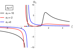
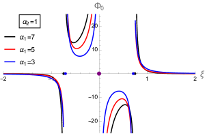
a)    b)    c)    d)

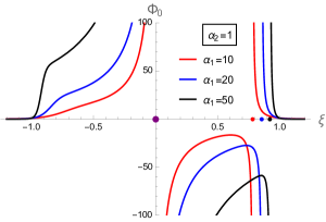
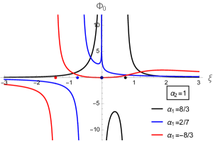
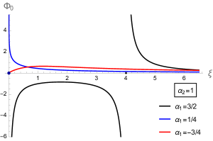
e)   f)    g)    h)

Figure 1: Plots of function $\Phi_{0}(\xi)$ of Eq. (26) for $\alpha_{2}=1$. Colored dots refer to the asymptotes location evinced through Propositions 1 and 3 given in Subsection IV.1. a) $\alpha_{1}$ negative odd integer; b) $\alpha_{1}$ negative even integer; c) $\alpha_{1}$ positive odd integer; d) $\alpha_{1}$ positive even integer; e) Birth of a step for higher values of $\alpha_{1}$ positive even integer; f)-h) Rational values $\alpha_{1}=q/p$ with $q$ and $p$ integers s.t. $\gcd(q,p)=1$: f) $q$ and $p$ both odd; g) $p$ odd and $q$ even; h) $p$ even and $q$ odd.

The remaining three plots, Figs. 1.f)-h), deal with the case $\alpha_{1}\in\mathbb{Q}$, thus relying on Propositions 3 and 4 in Subsection IV.1. To proceed, we assign to each $\alpha_{1}\in\mathbb{Q}$ a unique pair of integers $q,p$ such that $\alpha_{1}=q/p$, with $p>0$ and $\gcd(q,p)=1$. When $q$ and $p$ are both odd the analogy is with the case of odd integers $\alpha_{1}$. Precisely, if $q$ is odd positive (see black curve in Fig. 1.f)) then the behavior resembles the one of of Figure 1.c) for odd integers $\alpha_{1}>1$. In a similar way, when $q$ is an odd negative (red curve in Fig. 1.f) the likeness is with 1.a) treating odd negative integers $\alpha_{1}$. Correspondingly, when $p$ is odd and $q$ is even, the behavior of even integers $\alpha_{1}$ is recovered. For instance, when $\alpha_{1}<0$ the curves originating for $\Phi_{0}(\xi;\alpha_{1},1)$ (red curve in Fig. 1.g)) are alike those for negative even $\alpha_{1}$ in Fig. 1.b). On the contrary, for positive $\alpha_{1}<0$ (black curve in 1.g)) the resemblance is with shapes arising for even positive $\alpha_{1}$ (Fig. 1.d)). Outcomes when $0<\alpha_{1}<1$ have to be commented separately. Blue curves in Figs. 1.f)-h) show the singularity at the origin $\xi^{(0)}=0$, and possibly a second one at $\xi_{-}^{c}$ if $p$ and $q$ are odd and even, respectively. In the latter occurrence, the singularity at $\xi_{-}$ remains visible for small values of $\alpha_{1}$, in that $\xi_{-}=-|(\alpha_{1}-1)\alpha_{2}|^{\frac{1}{1-\alpha_{1}}}\simeq-|\alpha_{2}|$. In contrast, $\xi_{-}\to 0^{-}$ when $\alpha_{1}$ approaches the unity from below.

The scenario arising for functions $\Phi_{0}(\xi)$ given by Eq. (26) with negative values of $\alpha_{2}$ can be understood from Figure 2. We proceed concisely on the grounds of symmetries and analitical information gained for $\alpha_{2}>0$. We start with by remarking indeed that for $\alpha_{2}<0$ and integers $j$

$$\Phi_{0}(\xi;2j,\alpha_{2})=-\Phi_{0}(\xi;2j,-|\alpha_{2}|)\,\,.$$ (28)

Therefore, curves for $\Phi_{0}$ when $\alpha_{2}<0$ and $\alpha_{1}$ are even integers result from plots b) and d) of Figure 1 upon performing joint reflections $\xi\to-\xi$ and $\Phi_{0}\to-\Phi_{0}$. As for negative odd integers $\alpha_{1}$, the two vertical asymptotes in Figure 2.a) are placed at $\xi_{\pm}$. Opposite to Fig. 1.d) which also furnished us two-asymptote depiction for the function $\Phi_{0}$, there is no trait designing a stationary point. Finally for the case $\alpha_{2}<0$, one asymptote and two monotonically growing curves are typified by positive even integer values of $\alpha_{1}$, Figure 2.b).

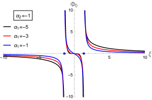
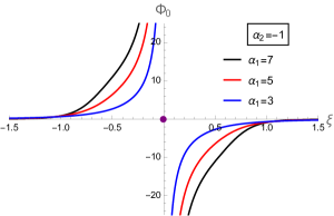
a)    b)

Figure 2: Plots of function $\Phi_{0}(\xi)$ of Eq. (26) for $\alpha_{2}=-1$. Colored dots refer to the asymptotes location. a) $\alpha_{1}$ negative odd integer; b) $\alpha_{1}$ positive odd integer.

V Solutions (21) to Equation (1) when $\Delta=0$

The clarification of the behavior allowed for $\Phi_{0}(\xi)$ put the basis for the understanding of solutions $v(x,t)$ to Equation (1) that are or the form (21) and pertinent to the case $\Delta=c_{1}^{2}c_{4}+c_{2}c_{3}^{2}=0$. While conveying particulars of $\Phi_{0}(\xi;\alpha_{1},\alpha_{2})$ to solutions of (1) via (21), values and signs of constants $c_{j}$ clearly matter. The role of the evolutionary variable $t$ is also evident in altering the magnitude and moving the poles of resulting solutions $v(x,t)$. As a matter of fact, the changeover from the similarity coordinate $\xi$ to the original independent variables $x$ and $t$ implies that to every point in the $\xi$-axis it is associated a curve $x(t)$ in the $(t,x)$ plane (at $t\neq 0$): the straight line $c_{1}x=c_{2}t$ for the point $\xi=0$, and the composition

$$x(t)=\frac{1}{c_{1}}\left(c_{2}t+\frac{\xi}{Bt}\right)\,\,$$ (29)

of the same translational motion with an hyperbolic curve for any other point $\xi$. Hence

1. when $\xi/Bc_{1}$ and $c_{2}/c_{1}$ are both strictly positive, then $x(t)$ is strictly positive (negative) over all the positive (negative) $t$-domain;

2. if $\xi/Bc_{1}>0$ and $c_{2}/c_{1}<0$, then $x(t)>0$ when either $t<-\sqrt{-\xi/Bc_{2}}$ or $0<t<\sqrt{-\xi/Bc_{2}}$;

3. if $\xi/Bc_{1}<0$ and $c_{2}/c_{1}>0$, then $x(t)>0$ when either $-\sqrt{-\xi/Bc_{2}}<t<0$ or $t>\sqrt{-\xi/Bc_{2}}$;

4. if $\xi/c_{1}$ and $c_{2}/c_{1}$ are both strictly negative, then $x_{s}$ is strictly negative (positive) over all the positive (negative) $t$-domain;

5. if $\xi=0$, then ${\rm sign}(x(t))={\rm sign}(c_{1}c_{2}t)$.

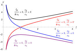
a

Figure 3: Qualitative motion for $t>0$ of a point $\xi_{p}$ on the $\xi$-axis as it is implied by Equation (29). Case i) (black): $\xi_{p}/Bc_{1}>0$ and $c_{2}/c_{1}>0$; Case ii) (blue): $\xi_{p}/Bc_{1}>0$ and $c_{2}/c_{1}<0$; Case iii) (red): $\xi_{p}/Bc_{1}<0$ and $c_{2}/c_{1}>0$; Case iv) (purple): $\xi_{p}/Bc_{1}<0$ and $c_{2}/c_{1}<0$.

Qualitative behavior of $x(t)$ concerned with $\xi\neq 0$ is summarized in Figure 3. In particular, the above schematics apply to connote the relocation on the $x$-axis of singularities of similarity solutions (21) while $t$ varies. We thus see that in cases i) and iv) the same value of $x$ can be obtained for two distinct values of the local variable $t>0$, meaning that a reversal of the singularity motion is exhibited. In cases ii) and iii), instead, there is a one-to-one correspondence based on a monotonic behavior for the function $x(t)$ of Equation (29).

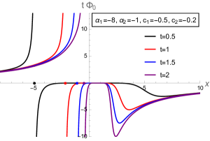
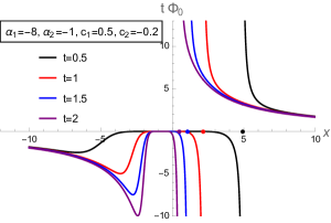
a)    b)

Figure 4: Examples of graphs of function $t\Phi(x,t)$ that follows from (26) at different times and for different choices of parameters $c_{1}$ and $c_{2}$. Equation (26) has been taken with $\alpha_{1}=-8$ and $\alpha_{2}=1$, for which the shape of $\Phi(\xi)$ is analogous to curves of Fig. 1.b). Colored dots refer to the asymptotes location. a) Progressive deformation of shape for $t\Phi(x,t)$ when $c_{1}$ and $c_{2}$ are both negative. b) Progressive deformation of shape for $t\Phi(x,t)$ when $c_{1}>0$ and $c_{2}<0$.

We are now in the position to outline more efficiently the significant aspects of similarity solution (21) when $\Delta=0$. Regardless obvious remarks in respect of consequences due to signs of the constants $c_{j}$, it is helpful to consider an example of just the function $t\Phi_{0}=t\Phi_{0}(x,t)$. In Figure 4, a case based on curves $\Phi$ of the type Fig. 1.b) is considered, in particular by setting $\alpha_{1}=-8$ and $\alpha_{2}=1$. Plots there supply a glimpse into effects of sign changes for the constants $c_{1,2}$ at positive $t$. For completeness, and being more instructive, the spectrum of the real “evolutionary” variable $t$ shall be permitted to comprise negative values. To this, we will consider coefficients $c_{1}$ and $c_{2}$ be both positive, as shown in Figure 5. In the formal limit $t\to-\infty$, resulting function $t\Phi_{0}(x,t)$ is null. For negative but increasing $t$’s, profiles like curves in Figure 1.b) tend to form, with lower and lower values attained by the maximum which moves to the right becoming smoother. The generated asymptote first moves to the right either, then reverses its motion by progressively placing itself at lower and lower values of $x$. At $t=0$, the asymptote and the maximum (experiencing the ongoing magnitude suppression) are pushed at infinity, and the function lies again on the $x$ axis. At later $t$, curves are no longer similar to those of Fig. 1.b), but rather to those ones one gets from them through the simultaneous reflections about horizontal and vertical axes. An asymptote is brought back in the picture from $\infty$, approaching a stationary point which is reinstated, but as as a minimum moving from $-\infty$ towards the direction of the increasing $x$ becoming narrower and narrower. The asymptote again experiences a “bouncing back” mechanism and an inversion of its motion, but without starting to departing from the minimum (see Fig. 5). In the formal asymptotic limit $t\to\infty$, the curve again flattens down on the abscissa. Analogous analysis can be worked out by chosing other pairs of parameters $\alpha_{1}$ and $\alpha_{2}$.

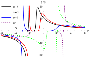
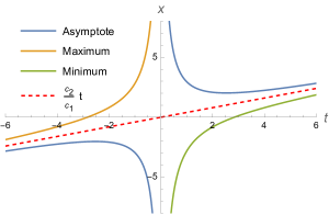
a)     b)

Figure 5: Asymptotes and stationary points motion for the function $t\Phi(x,t)$ arising from (26) with $\alpha_{1}=-8$, $\alpha_{2}=1$, $c_{1}=0.5$ and $c_{2}=0.2$. a) The function $t\Phi_{0}$ for different values of $t$. For increasing negative $t$ the maximum flattens and shifts the location to higher values of the coordinate $x$. The asymptote moves as well, but after moving to the right on the $x$-axis (see the red curve determined at $t=-3$ on the right of the black one obtained for $t=-4$) it reverses its motion and directs itself to the opposite direction (see the blue curve at $t=-1$ on the left of the previously mentioned black and red ones). b) Motion in the $(t,x)$ plane of asymptote and stationary points, signalling the inversion of motion only for the former.

VI Properties of Equation (24) and its solutions

Evidently, Equation (24) is a non-trivial nonlinear ODE. Contrary to Equation (24), we have not found a transformation connecting it to the list of Painlevé equations. Of course approximate methods can be resorted in the attempt to have a glimpse of possible dynamics emerging from it. For instance, Painlevé-like test arguments (see e.g. conte ; hone and Refs. therein for an account on this subject) can be carried out while aimed at highlighting features of its solutions, such as their singularity structure. A priori Equation (24) can have solutions with movable singularities which vary with the initial conditions. Testing the singularity structure of the equation appears particularly meaningful, as it is natural to wonder about admissible deviations and generalizations with respect to the very basic case (18) displayed, for the one-dimensional reduction of the problem discussed in Subsection III.1. Having this in mind, the formal expansion

$$\Phi(\xi)=(\xi-\xi_{0})^{-j}\sum_{k=k_{0}}^{\infty}f_{k}\,\,(\xi-\xi_{0})^{k}\,\,,$$ (30)

being the $f_{k}$’s constants, can be thence resorted to identify all possible dominant balances, i.e. the singularities whose form behaves like $\Phi\propto(\xi-\xi_{0})^{-j}$. It is readily seen that demanding $j$ to be a positive integer leads to the identification $j=1$, so that the singular dominant behavior is associated with a single pole. Going further in the analysis, the resonance $r=1$ is found (in addition to $r=-1$). So, the two arbitrary constants entering the Laurent series representation of the solution (30) with $j=1$ are given by the movable pole $\xi_{0}$ and the coefficient $f_{1}$. To our aims, it is significant to focus on the role of dominant term about a singular point $\xi_{0}$ in the local representations of $\Phi$,

$$\Phi(\xi)\cong\frac{1}{\xi-\xi_{0}}\,\,.$$ (31)

That is, for (21) and assuming $\Delta\neq 0$, we can take for Eq. (1) the approximate solution

$$v(x,t)\cong\frac{\eta\sigma c_{1}\,t}{t(c_{1}x-c_{2}t)-\xi_{0}^{*}}=\frac{\eta\sigma}{x-x_{s}(t)}$$ (32)

about a singular point (the term $\sigma c_{3}/c_{1}$ can be patently omitted), being $\xi_{0}^{*}=\eta^{2}c_{1}^{3}\Delta^{-1}\,\xi_{0}$ and $x_{s}(t)$ given by formula (29) with $\xi/B\to\xi_{0}^{*}$, i.e.

$$x_{s}(t)=\frac{1}{c_{1}}\left(c_{2}t+\frac{\xi_{0}^{*}}{t}\right)\,\,$$ (33)

($c_{1}\neq 0$). At any given $t\neq 0$, the singularity shows up when the real variable $x$ attains the finite value $x_{s}(t)$. When $\xi^{*}_{0}=0$, the pole $x_{s}(t)$ simply depends linearly on $t$ and translates with constant velocity $c_{2}/c_{1}$. If $\xi_{0}^{*}\neq 0$ the quantity $x_{s}$ can be positive or negative depending on the signs of $\xi_{0}^{*}/c_{1}$ and $c_{2}/c_{1}$. The motion of poles of the rational solution (32) is easily inferred. We thus see that when $\xi_{0}^{*}/c_{1}$ and $c_{2}/c_{1}$ are either both positive or both negative (cases i) and iv) of previous Section) the same value of $x_{s}$ can be obtained for two distinct values of the local variable $t>0$, meaning that a reversal of the pole motion is exhibited. When $\xi_{0}^{*}/c_{1}>0$ and $c_{2}/c_{1}<0$ or $\xi_{0}^{*}/c_{1}<0$ and $c_{2}/c_{1}>0$ -cases ii) and iii)- there is instead a one-to-one correspondence based on a monotonic behavior for the function $x_{s}(t)$. Qualitative behavior of $x_{s}(t)$ when $t>0$ and $\xi^{*}\neq 0$ is as in Fig. 3. Also remark that when $\Delta=c_{1}^{2}c_{4}+c_{2}c_{3}^{2}=0$ the coefficients $c_{3}$ and $c_{4}$ play no role on the identification and on the motion of the pole $x_{s}(t)$ as they do not enter in the definition of neither the variable, which now reads $\xi=t\,(c_{1}x-c_{2}t)$, nor in defining a normalized value $\xi^{*}_{0}$ of the pole $\xi_{0}$ (since now one would have (29) with $\xi\to\xi_{0}$).

To gain a picture of how its solutions evolve away from a singularity of the type (31), a numerical integration of equation (22) can be performed. Remark that Equation (22) does not admit invariance neither under reflections $\xi\to-\xi$ nor under translations $\xi\to\xi+\delta\xi$.

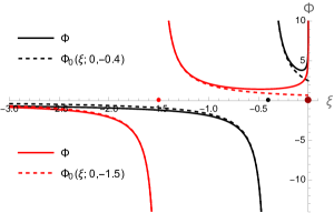
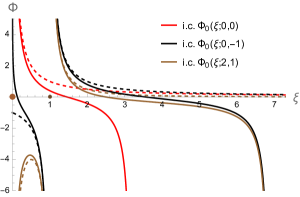
a)      b)

Figure 6: Numerical integration of Eq. (22) upon superimposition of initial conditions based on functions (26) for distinguished choices of parameters. Functions used to set initial conditions are represented by the dashed curves. a) Negative simple poles in $\xi_{0}=-0.4$ (black) and $\xi_{0}=-1.5$ (red). b) Comparison of curves obtained by superimposing initial conditions either matching simple pole functions at $\xi_{0}=0,1$ (red and black curves, respectively) or (26) with $\alpha_{1}=2$ and $\alpha_{2}=1$ (brown) which possess both those singularities.

Figure 6 pertains solutions $\Phi$ to Equations (24) obtained with initial condition of the simple pole type about $\xi_{0}<0$. That is, initial conditions have been imposed by assigning that, at a point very close to a certain $\xi_{0}>0$, solutions $\Phi$ and $\Phi^{\prime}$ assume the same values of the function $(\xi-\xi_{0})^{-1}$ and of its differential. The initial condition matching takes place very close to singularities and for solutions values rather above the domain considered in plots. Integration is performed by increasing the variable $\xi$ from a pole until a successive singularity develops. Numerical integration of (24) in the positive and negative domains of the variable $\xi$ are performed separately. In particular, Figure 6.a) refers to the case $\xi_{0}<0$. To the left of this singularity, solutions essentially comply with the simple pole function $(\xi-\xi_{0})^{-1}$. The plot also tells how the solution runs to a novel singularity located at the origin. When $\xi$ increases and begins to be distant enough from $\xi_{0}<0$ the memory of the pole begins to get lost, and a change of convexity anticipates a growth at a noticeably high rate while approaching the singular point $\xi=0$. Red and black curves in Figure 6.b) report results one obtains by integrating Equation (24) over the domain $\xi>0$ after superimposing initial conditions of the simple pole type $\Phi\simeq(\xi-\xi_{0})^{-1}$, with $\xi_{0}>0$. After increasing $\xi$ a while, the portion of solutions that develops to the right of the point $\xi_{0}>0$ are pushed down and directed to a singular behavior, with a character resembling to $\tan$-type functions. A translation of the singular point $\xi_{0}$ provokes a dilation of the interval between the initial and the newly formed singularities (see the red and black curves in curves in 6.b)). Confronted with (23) with the same initial conditions, it can be thus concluded that there is a substantial role played by the last term in Equation (24) that sustains the generation of an additional singularity at the origin $\xi=0$.

VI.1 Sensitivity to initial conditions

Discussing solutions to Equation (24) would clearly benefit of taking into account initial conditions other than those used so far. At the beginning of this Section, we have seen that simple pole behavior can be extracted for solutions to Equation (24). But we have also learned in Section IV how singularities of different types originate for functions $\Phi$ when $\Delta=0$. It makes therefore sense to look at solutions to Equation (24) based on sampling of initial conditions establishing a more direct connection with general solutions to the problem (23). For instance, we set initial conditions for (24) demanding solution values and their first derivatives as given by the function (26) near a singularity. After doing so, families of numerical solutions to Equation (24) follow that can be seen as deformations of the solutions (26), from which they are expected to inherit some major features. Figure 6.b) considers also what is obtained by this strategy. While not a substantial dependence on this new initial condition, compared to the simple pole initial condition, is displayed to the right of the singularity (see the brown and black $\tan$-type shapes on the right of Figure 6.b)), quite a difference is manifested on its left side. As solid and dotted brown curves in Figure 6.b) show for smaller $\xi$, solutions to (24) associated with initial data as given by $\Phi_{0}$ tend to stay adherent to $\Phi_{0}$ itself, thence preserving their same singular behavior approaching the origin. A striking dissimilarity is presented instead in the same domain between the origin and the singularity for the solution. Starting from the left of the singularity to the origin, the solution to (24) (left solid black curve for small values of $\xi$) leaves the $(\xi-\xi_{0})^{-1}$ curve (dotted black) determining its initial simple pole imprinting so to generate again a singularity at the origin, but this time progressing to the positive infinity value through a $\tan$-type profile.

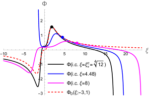
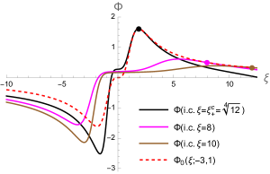
a)    b)

Figure 7: Comparison between functions solving (24) and solution (26) pertinent to $\Delta=0$. $\Phi(\xi)$ and $\Phi_{0}(\xi;-3,1)$ are required to pass both through chosen individual points (colored disks) with the same rate. The black curve denotes the solution demanded to possess the same maximum (black disk) of $\Phi_{0}(\xi;-3,1)$ (red dashed) at $\xi=\xi_{+}^{c}=12^{1/4}$. a) Deformation of the reference profile $\Phi_{0}(\xi;-3,1)$ and sudden apparence of a dissimilar curve (blue). b) Dynamics of the minimum by varying initial conditions. Lowering the maximum does not necessarily introduce an overall smoothing of $\Phi$ in the $\xi<0$ domain (compare magenta and brown curves).

Having payed attention on consequences of initial conditions near the singularity, devised on the observation of dominant term (31) and solutions to (23), in order to having a more complete picture on the problem (24), it is worth to pursue the same strategy of screening the solutions that are isolated by the enforcement of data similar to that of an assigned reference function (26). However, at this time data are taken at some point far from singularities of $\Phi_{0}$. Stationary points can be chosen as reference for initial conditions, for instance. In Figure 7, in particular, the solution to (24) is asked to develop the same local maxima of the function (26) with the off $\alpha_{1}=-3$ and $\alpha_{2}=1$ (red dashed). A curve emerges that is not anymore anti-symmetric with respect to the vertical axis, and an asymptote comes after the maximum in a manner analogous to what we have formerly seen to progress from a superimposed vertical asymptote, see Fig. 6.b). To some extend, the $\Phi_{0}$-pattern is better preserved before the maximum, albeit it is evident that also the anti-symmetry between the maximum and the minimum breaks down. The latter is visibly lowered, like most of the curve in the $\xi<0$ domain. The raising of the function to positive values in the proximity of the origin is also clear, and this contributes to the formation of a greater dip conducting to the minimum.

Graphs of Figure 7 also illustrate what can be displayed by still taking $\Phi_{0}(\xi;-3,1)$ as trial function to settle initial conditions for the ODE (24), but choosing points on it different from the maximum. In particular, we have considered points to the right of the maximum, where the function smoothly decays monotonically. With the diminishing of $\Phi_{0}(\xi;-3,1)$ and $\Phi^{\prime}_{0}(\xi;-3,1)$ there is a general tendency to push down the maximum for $\Phi$, which moves uniformly to the right, see magenta and brown curves in Figures 7.a)-b). A memory of the minimum developing for $\Phi_{0}(\xi;-3,1)$ is also seen, but in the region $\xi<0$ the function $\Phi$ does not experience the same flattening effect taking place for $\xi>0$; see the magenta curve in Figure 7.a). Actually, Figure 7.b) shows that while the right part of the curve $\Phi$ attains lower values for smoother initial conditions (magenta and brown disks), the left part does not: the minimum for the magenta curve is actually less peaked than that of the brown curve which also tends to get back closer to origin. Also remark that the output profile for $\Phi$ can change abruptly in correspondence of certain initial conditions. This is shown by means of the blue curve in Fig. 7.a) whose shape evidently reminds the portion of $\Phi_{0}$ developing on the right of the singularity for even negative $\alpha_{1}$ and $\alpha_{2}=1$, but with in addition the newly introduced movable singularity standing out for positive $\xi$. This can be intuitively understood on the grounds that the choosing of initial conditions for $\Phi$ and $\Phi^{\prime}$ may in practice act as selecting a $\Phi_{0}$ with different pairs of $\alpha_{1}$ and $\alpha_{2}$.

VI.2 Remarks on solutions (21) to (1) for $\Delta\neq 0$

We have previously gained an insight on some peculiarities of a class of solutions to (22) and the next step would be arguing the pulling back to the original equation (1) acted via (21). The analysis of the effects on solutions to (1) can be prospected straight away founded on observations and guiding route put together for the case $\Delta=0$ treated in Section IV. We shall not argue therefore the complete casistics for the choices that can be made for the coefficients $c_{j}$ for it is very intelligible from (21). In Figure 8, we therefore produce only the function $t\Phi$ determining solutions to (1) from the solution to (24) drawn in Figure 7. The predicted flattening out during the evolution near $t=0$, the exchange with reflections between the quadrants of the curve sections after the annulment at $t=0$ and the amplification of the peaks in the later evolution are manifest. We conclude the Section by emphasizing that in potential applicative problems relying on equation (1) it may be also necessary to ascertain the consistency with possible constraint on domains of variables for the specific subject matter under study. For instance, if $v$ is definite positive, those portions of the $\Phi$ curves have to be selected such that also the condition $v\geq 0$ comes true. Depending on the signs of structural coefficients $c_{j}$’s, in turn this demands taking into account either the condition $B\eta\frac{c_{1}^{2}}{c_{3}}t\Phi<1$ or the condition $B\eta\frac{c_{1}^{2}}{c_{3}}t\Phi>1$, where $B=1$ if $\Delta=0$ or $B=\Delta\eta^{-2}c_{1}^{-4}$ otherwise (Eq. (25)); i.e., either $\eta\frac{c_{1}^{2}}{c_{3}}t\Phi>1$ or $\eta\frac{c_{1}^{2}}{c_{3}}t\Phi<1$ for $\Delta=0$, and either $\frac{\Delta}{\eta c_{1}^{2}c_{3}}t\Phi>1$ or $\frac{\Delta}{\eta c_{1}^{2}c_{3}}t\Phi>1$ if $\Delta\neq 0$.

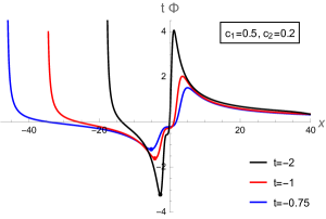
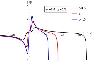
a)    b)

Figure 8: Examples of function $t\Phi(x,t)$ that conseque from (24) at different times and for $c_{1}=0.5$, $c_{2}=0.2$ and $\Delta=\eta^{2}c_{1}^{4}$. Colored dots refer to the inital value assignment for the function $\Phi$ coinciding with the maximum of (26) with $\alpha_{1}=-3$ and $\alpha_{2}=1$. a) Negative $t$. b) Positive $t$.

VII N-pole dynamics of rational solutions

By looking at the Equation (1) from the angle of local symmetry properties and similarity solutions, we have gained through the reduction (21) an interesting perspective on some pivotal characteristics owned by its solutions. The study we presented is clearly of limited extend, and the investigation of other fundamental features is in order. Among the open problems there is, for instance, the comprehension of aspects such as the existence of other distinctive classes of solutions and the possibility to proceed with their classification. In particular, shedding light on the existence of rational solutions comprising multiple simple poles seems to be a naturally due development. Indeed, singular solutions to remarkable integrable equations and their pole dynamics have proved to be intriguingly linked to the dynamics of particles in many-body systems (see, for instance, the seminal papers airault ; Choodnovsky ; calogero 2 ) as well as to rogue waves (see dubard2 ; gaillard ; clarkson2 ), and are still subject of active investigations about the rational solutions in the KP hierarchy and Painlevé equations zabrodin2019 ; zabrodin2020 ; zabrodin2021 ; clarkson3 . In addressing this issue, guidelines can be taken from discussions concerning other integrable equations, as put forward for instance in Choodnovsky . The most natural connection in this respect clearly is seized with the standard Bateman-Burgers equation. In such a case, the existence of rational solutions and the analysis of their poles properties has been nicely investigated in deconinck , for instance. By proceeding similarly to Choodnovsky ; deconinck , the $N$-pole ansatz

$$v(x,t)=\eta\sigma\sum_{k=1}^{N}\frac{R_{k}(t)}{x-x_{k}(t)}$$ (34)

can be substitued in (1), and by later setting $x=x_{j}+\epsilon$, the resulting equation can be expanded in powers of $\epsilon$. As in the Bateman-Burgers case, equating the most singular terms prompts to $R_{k}(t)=1$. We observe here, however, that quite a more complex pole dynamics is suggested for rational solution of Equation (1), at least when $\Delta\neq 0$. Indeed, by collecting terms at the successive order, one finds that the motion of poles $x_{k}(t)$ superimposed via (34) can be thus ascribed, at this level of approximation, to the concurrence of two mechanisms: a translation at fixed constant speed unavoidably entering in the matter once $c_{1}c_{4}\neq 0$, and an additional motion obeying a nontrivial differential system. That is:

$$x_{k}(t)=-\frac{c_{1}c_{4}}{c_{3}^{3}}\,t+y_{k}(t)=\left(\frac{c_{1}}{c_{2}}-\frac{\Delta}{c_{1}c_{3}^{2}}\right)t+y_{k}(t)\,\,,$$ (35)

where the functions $y_{j}(t)$ are determined by solutions of the following dynamical system:

$$\dot{y}_{k}(t)= \frac{\Delta}{c_{3}^{3}}\sum_{m=1}^{N-1}(m+1)!\left(-\frac{c_{1}}{c_{3}}\right)^{m-1}\,\eta^{m}\,{\cal P}^{(m)}_{k}\left[\{y_{m}\}_{1}^{N}\right]\,\,,\qquad\qquad\left(\dot{}=\frac{d}{dt}\right)\,\,,$$ (36)

the ${\cal P}^{(m)}_{k}$’s denoting the sum of products of distinct terms $(y_{k}-y_{j})^{-1}$, i.e.

$${\cal P}^{(1)}_{k}\left[\{y_{m}\}_{1}^{N}\right]=\sum\limits_{\begin{subarray}{c}j=1\\ i\neq k\end{subarray}}^{N}\frac{1}{y_{k}-y_{j}}\,\,,\qquad{\cal P}^{(2)}_{k}\left[\{y_{m}\}_{1}^{N}\right]=\sum\limits_{\begin{subarray}{c}j,m=1\\ j,m\neq k\\ j\neq m\end{subarray}}^{N}\frac{1}{(y_{k}-y_{j})(y_{k}-y_{m})}\,\,,$$ (37)

$${\cal P}^{(3)}_{k}\left[\{y_{m}\}_{1}^{N}\right]=\sum\limits_{\begin{subarray}{c}j,m,r=1\\ j,m,r\neq k\\ j\neq m,j\neq r,m\neq r\end{subarray}}^{N}\frac{1}{(y_{k}-y_{j})(y_{k}-y_{m})(y_{k}-y_{r})}$$ (38)

and so forth. The situation is therefore much different from the standard Bateman-Burgers equation with diffusivity $\eta$ issuing for $c_{1}\to 0$ (along with the normalization conditions $c_{3}=-c_{2}$ and $\sigma=-2$), for which the motion of poles entering a N-pole ansatz of the type (34) would be determined by the hamiltonian differential system $\dot{x}_{k}(t)=-2\eta{\cal P}^{(1)}_{k}\left[\{x_{m}\}_{1}^{N}\right]$. Then, there is an interaction among poles that is not limited to just pairwise couplings as it happens in the standard Bateman-Burgers equation deconinck . The manner in which a pole $x_{k}(t)$ in (34) varies is ruled by its correlations with an increasing number of the other distinct poles, until all the poles appear. Two remarks are clearly in order on this statement. First, it has been assumed that $\Delta=c_{1}^{2}c_{4}+c_{2}c_{3}^{2}\neq 0$. When $\Delta=0$ one is merely lead instead to $t$-linear translations of poles with rate $\dot{x}_{k}(t)=\frac{c_{2}}{c_{1}}t$. Secondly, under the circumstance that $\eta$ is a small perturbation parameter, one may reason about disregarding higher-order terms in powers of $\eta$. By maintaining only the lowest order term in the right hand side of (36), the dynamical system governing the contribution $y_{k}(t)$ to the motion of poles $x_{k}(t)$ shares essentially the same form found in the Bateman-Burgers case:

$$\dot{y}_{k}(t)=2\frac{\Delta}{c_{3}^{3}}\eta\,{\cal P}^{(1)}_{k}\left[\{y_{m}\}_{1}^{N}\right]\,\,.$$ (39)

The investigation of the differential system (36) goes beyond our current scopes. We limit ourselves to remark that complete integrability is expected to be evincible using the Cole-Hopf transformation and the relationship between equations (1) and (5).

VIII Discussion and conclusions

In this communication, we have addressed the study of the nonlinear 1+1 dimensional partial differential equation (1), i.e.

$$\partial_{t}v+\partial_{x}\left\{\frac{1}{c_{1}v+c_{3}\sigma}\left[c_{2}v^{2}+c_{4}\sigma^{2}+\sigma\eta\left(c_{1}\partial_{t}v+c_{2}\partial_{x}v\right)\right]\right\}=0\,\,,$$

representing a non-evolutive generalisation of known diffusive/dissipative equations. The equation has been introduced recently in giglio and ensues from rather general grounds. Indeed, it can be obtained from a 1+1 differential conservation law where: i) the flux density depends both on the density and (linearly) from the first derivatives of density with respect to the local variables; ii) the linearisability via a Cole-Hopf transform is demanded in addition. To date, very little is known on Equation (1) and its solutions. When one or more of the coefficients $c_{j}$ do vanish, some crucial simplifications may occur that enable to determine solutions almost effortlessy, as we commented in Subsection II.1. In particular, the simple $\tan$-type (17) or rational solutions (18) are admitted. The circumstance definitively motivates the paying attention on the occurrence of singularities for solutions to (1).

In the present communication, by performing a similarity reduction dictated by one of the local symmetry generators underlying the equation (1), we have shown that a nonlinear ordinary differential equation arises which is connected to the Painlevé III equation. While standard arguments concerning the existence of solutions with simple poles prove their usefulness, the discussion we presented here in this regard took quite a benefit from the circumstance that the model is exactly solvable in the special case where the constraint $\Delta=c_{1}^{2}c_{4}+c_{2}c_{3}^{2}=0$ do hold. The general real solution thence originated takes a simple mathematical structure with a still rich dynamics and interesting key-elements, e.g. in respect to the presence of singularities how we have detailed. Regardless the potential marginal relevance of such a strict binding $\Delta=0$ in concrete applications to specific problems, the circumstance of exact solvability provides indeed first remarkable hints concerning what to expect for solutions to the general differential problem when $\Delta\neq 0$, at least within fairly identified assumptions and regimes. This allows for gaining a clue also on the unavoidable qualitative differences, such as the generation of additional divergences, as we argued in Section VI where the strategy of selecting solutions by tailoring them to an assigned solution pertaining $\Delta=0$ has been pursued. We have been also attentive to the implications in respect to the $t$-dependent dynamics of poles and asymptotes for the solution, showing an inversion of their motions. These results put a basis for the understanding of the general case $\Delta\neq 0$, for which a more singular behavior has been shown to emerge.

Future investigations concerned with (1) are definitively in order and they may naturally include both other mathematical issues and more applicative problems. We already understood in Section VII that a deeper comprehension of the integrability properties underlying the dynamics of multiple poles would be desirable, in a manner parallel to what has been done for the Bateman-Burgers equation for instance deconinck . Another elucidation looks to be in respect to the identification of non-local symmetries. Besides providing insights on the possibility to have receipts for transferring possible analytical results, hints on the settling of diverse coordinate transformations may play a role as regards aspects like the reduction to normal form, classification of solutions and characterization of possible correlated hierarchies in a way similar to the case of the non-evolutionary viscous scalar reduction of the two-component Camassa-Holm equation considered in arsie . Generalised symmetries determining Miura-type actions play indeed a decisive role in that framework. It would be also interesting to understand if they may enable to connect (1) to a Painlevé equation in the general case when $\Delta\neq 0$, as we have seen that for $\Delta=0$ the equation is related to the Painlevé III through a Cole-Hopf type transformation. Other developments may be more focused on the application of Equation (1), including those for purposes potentially different from the fluid systems considered so far, such as in the context of complex systems based on mean-field spin models. The idea of formally describing the governing behavior of relevant statistical quantities through the solutions of PDEs is starting to be appraised even for problems in reaction kinetics agliari2018 and artificial intelligence agliari2022 , for instance. This may raise the question about the possible need to implement the model (3) while dealing with specific problems, such as by taking into account other non-local terms in the expansion that may cure or smoothen appearing criticalities and allow for the identification of multiple scales of both mathematical and applicative relevance. We finally mention that natural advances of the investigation performed in this work entail multi-component integrable conservation laws, for instance those arising in the treatment of nematic liquid crystal systems dematteis ; dematteis2 . Extension of our approach to integrable hydrodynamic chains may also prove to be insightful, e.g. in the context of random matrix models benassi .

Appendix A Proofs of Proposition 2, Proposition 3 and Proposition 4

Proposition 2 (Stationary points of solution (26) for integer values of $\alpha_{1}$).

Let $\alpha_{1}\in\mathbb{Z}$, $\alpha_{2}>0$, $\xi^{(0)}=0$ and $\xi_{\pm}^{c}=\pm|\alpha_{1}(1-\alpha_{1})\alpha_{2}|^{\frac{1}{1-\alpha_{1}}}$. The stationary points of solution (26) are listed below.

1. Three stationary points located at $\xi=\xi^{(0)}$ (inflection point) and $\xi=\xi_{\pm}^{c}$ for $\alpha_{1}$ odd negative integer with $\alpha_{1}<-1$.

2. Two stationary points when $\alpha_{1}=-1$, located at $\xi=\xi_{\pm}^{c}$ .

3. Two stationary points for $\alpha_{1}$ even negative integer, located at $\xi=\xi^{(0)}$ and $\xi=\xi_{+}^{c}$.

4. One single stationary point located at $\xi=\xi_{+}^{c}$ for $\alpha_{1}$ even positive integer.

5. Two stationary points for odd positive integers $\alpha_{1}$ located at $\xi=\xi_{\pm}^{c}$.

Proof.

The proof is based on similar arguments used in Proposition 1. The stationary points of (26) are given by the zeros of $\Phi_{0}^{\prime}(\xi;\alpha_{1},\alpha_{2})=(\alpha_{1}-1)\frac{\left[\alpha_{1}(\alpha_{1}-1)\alpha_{2}\xi^{\alpha_{1}-1}-1\right]}{\left[(\alpha_{1}-1)\alpha_{2}\xi^{\alpha_{1}}-\xi\right]^{2}}$.
Let us first consider the case $\alpha_{1}\in\mathbb{Z}_{<0}$. The stationary points are given by the real roots of the polynomial $\mathcal{\tilde{P}}^{-}(\xi):=\left[\alpha_{1}(\alpha_{1}-1)\alpha_{2}-\xi^{1-\alpha_{1}}\right]\xi^{\alpha_{1}-1}$. One root $\xi^{(0)}=0$ arises for $\alpha_{1}<-1$. One can verify that $\Phi_{0}^{\prime\prime}(\xi^{(0)})=0$, hence giving an inflection point. The other roots for negative integers are given by $\xi_{l}=|\alpha_{1}(1-\alpha_{1})\alpha_{2}|^{\frac{1}{1-\alpha_{1}}}e^{i\frac{2l\pi}{1-\alpha_{1}}}$, $l=0,1,\cdots,-\alpha_{1}$. The real solution $\xi_{+}^{c}=|\alpha_{1}(1-\alpha_{1})\alpha_{2}|^{\frac{1}{1-\alpha_{1}}}$ is obtained when $l=0$, while $\xi_{-}^{c}=-|\alpha_{1}(1-\alpha_{1})\alpha_{2}|^{\frac{1}{1-\alpha_{1}}}$ is obtained for $\alpha_{1}$ odd when $l=\frac{1-\alpha_{1}}{2}$. These prove i), ii) and iii).
Let us now consider the case $\alpha_{1}\in\mathbb{Z}_{>0}$. The case $\alpha_{1}=1$ identifies the null solution as discussed earlier. When $\alpha_{1}>1$ we have that stationary points are real roots of the polynomial $\mathcal{\tilde{P}}^{+}(\xi):=\alpha_{1}(\alpha_{1}-1)\alpha_{2}\xi^{\alpha_{1}-1}-1$, $\xi_{l}=|\alpha_{1}(1-\alpha_{1})\alpha_{2}|^{\frac{1}{1-\alpha_{1}}}e^{i\frac{2l\pi}{1-\alpha_{1}}}$, $l=0,1,\cdots,\alpha_{1}-2$. We promptly identify the real root $\xi_{+}^{c}=|\alpha_{1}(1-\alpha_{1})\alpha_{2}|^{\frac{1}{1-\alpha_{1}}}$. A second real solution occurs for odd integers only, requiring $2l\pi=(1-\alpha_{1})\pi$, that is $l=\frac{1-\alpha_{1}}{2}$, giving $\xi_{-}^{c}=-|\alpha_{1}(1-\alpha_{1})\alpha_{2}|^{\frac{1}{1-\alpha_{1}}}$. These complete the proof of iv) and v).

∎

Proposition 3 (Singularities of (26) for rational values of $\alpha_{1}$).

Let $\alpha_{1}=\frac{q}{p}$ with $q,p\in\mathbb{Z}$ and $\gcd(q,p)=1$, and consider $\xi^{(0)}$, $\xi_{\pm}$ defined as in Proposition 1. The real poles of (26) are listed below.

1. Case $\alpha_{1}<0$.

   1. One singularity located at $\xi=\xi_{-}$ (branch point) if $p$ is odd and $q$ is even.

   2. No singularities if $p$ and $q$ are odd.

   3. One singularity at $\xi=\xi_{+}$ (branch point) if $p$ is even.

2. Case $0<\alpha_{1}<1$.

   1. Two singularities if $p$ is odd and $q$ is even located at $\xi=\xi^{(0)}$ (branch point) and $\xi=\xi_{-}$ (branch point).

   2. One singularity located at $\xi=\xi^{(0)}$ (branch point) if $p$ and $q$ are odd.

   3. One singularity located at $\xi=\xi^{(0)}$ (branch point) if $p$ is even.

3. Case $\alpha_{1}>1$.

   1. Two singularities if $p$ is odd and $q$ is even located at $\xi=\xi^{(0)}$ (pole) and $\xi=\xi_{+}$ (branch point).

   2. Three singularities if $p$ and $q$ are odd located at $\xi=\xi^{(0)}$ (pole) and $\xi=\xi_{\pm}$ (branch points).

   3. Two singularities at $\xi=\xi^{(0)}$ (pole) and $\xi=\xi_{+}$ if $p$ (branch point) is even.

Proof.

Wlog, let $p\in\mathbb{Z}_{>}0$ and consider the above different cases as $q$ varies in $\mathbb{Z}$. Note that for $p$ even, the solution (26) is defined for $\xi\geq 0$. Also notice that the additional condition $\gcd(q,p)=1$ ensures that to each $\alpha_{1}\in\mathbb{Q}$ we associate unambiguously a pair of integers $(q,p)$.
We will prove case iii) as an example, $\alpha_{1}>1$. In this case, singularities are given by zeros of the polynomial $\mathcal{P}^{+}(\xi):=\xi\left[\left((\alpha_{1}-1)\alpha_{2}\right)\xi^{\frac{q-p}{p}}-1\right]$. Clearly a singularity occurs at $\xi^{(0)}=0$. Other real solutions are among the following $\xi_{l}=|\alpha_{1}(1-\alpha_{1})\alpha_{2}|^{\frac{1}{1-\alpha_{1}}}e^{ip\frac{2l\pi}{q-p}}$, $l=0,1,\cdots,q-p-1$. Real roots are obtained in two cases, either looking for $l$ fulfilling $2pl=2k(q-p)$ or $2pl=(2k+1)(q-p)$ for some integer $k$. The former gives $\xi=\xi_{+}$, while the latter gives $\xi=\xi_{-}$. The parity of $q$ and $p$ implies the qualitative scenario. Indeed, $\xi=\xi_{+}$ arises for all parities of $q$ and $p$, but the situation is different for $\xi=\xi_{-}$. Indeed, only when $q$ and $p$ are both odd (hence $q-p$ even), an additional solution is found at $\xi=\xi_{-}$. This proves i).
Cases i) and ii) are derived following similar procedure and their proof is here omitted. In general, one has to identify the polynomial whose zero correspond to singularities of $\phi_{0}$, find the complex roots and select the real ones by looking at the parity of $q$ and $p$.

∎

Proposition 4 (Stationary points of (26) for rational values of $\alpha_{1}$).

Let $\alpha_{1}=\frac{q}{p}$ with $q,p\in\mathbb{Z}$ and $\gcd(q,p)=1$, and consider $\xi^{(0)}$, $\xi_{\pm}^{c}$ defined as in Proposition 2. The stationary points of (26) are listed below.

1. Case $\alpha_{1}<0$.

   1. Two stationary points located at $\xi=\xi^{(0)}$ and $\xi=\xi_{+}^{c}$ if $p$ is odd and $q$ is even.

   2. Three stationary points located at $\xi=\xi^{(0)}$ (inflection point) and $\xi=\xi_{\pm}^{c}$ if $p$ and $q$ are odd.

   3. Two stationary points located at $\xi=\xi^{(0)}$ and $\xi=\xi_{+}^{c}$ if $p$ is even.

2. Case $0<\alpha_{1}<1$.

   1. One stationary point at $\xi=\xi_{-}^{c}$ if $p$ is odd and $q$ is even.

   2. No stationary points if $p$ and $q$ are odd.

   3. No stationary points if $p$ is even.

3. Case $\alpha_{1}>1$.

   1. One stationary point located at $\xi=\xi_{+}^{c}$ if $p$ is odd and $q$ is even.

   2. Two stationary points located at $\xi=\xi_{\pm}^{c}$ if $p$ and $q$ are odd.

   3. One stationary point at $\xi=\xi_{+}^{c}$ if $p$ is even.

Proof.

Let $p\in\mathbb{Z}_{>}0$ and consider the above different cases as $q$ varies in $\mathbb{Z}$. We will prove case i) as an example, $\alpha_{1}<0$. In this case, stationary points are real zeros of the polynomial $P^{-}({\xi})=\xi^{-2\alpha_{1}}\left[\alpha_{1}\left(\alpha_{1}-1)\alpha_{2}-\xi^{1-\alpha_{1}}\right)\right]$. Clearly, $\xi=0$ is always a stationary point. The other stationary points are the real roots among $\xi_{l}=|\alpha_{1}(\alpha_{1}-1)\alpha_{2}|^{\frac{1}{1-\alpha_{1}}}e^{i\frac{2\pi lp}{p-q}}$, $l=0,1,\cdots,p-q-1$. Real roots are obtained in two cases, either looking for $l$ fulfilling $2pl=2k(q-p)$ or $2pl=(2k+1)(q-p)$ for some integer $k$. The former would imply $\xi=\xi_{+}^{c}$, while the latter would lead to $\xi=\xi_{-}^{c}$. A second stationary point located at $\xi=\xi_{+}^{c}$ arises for all parities of $q$ and $p$. A third stationary point located at $\xi=\xi_{-}^{c}$ arises when $p$ and $q$ are odd only, hence proving i). Cases ii) and iii) are derived following similar procedure and their proof is here omitted. ∎

- (1) F. Giglio, G. Landolfi and A. Moro, Integrable extended van der Waals model, Physica D 333, 293-300 (2016).
- (2) H. Bateman, Some recent research on the motion of fluids, Monthly Weather Review, 43, 163-170 (1915).
- (3) J.M. Burgers, Mathematical examples illustrating relations occurring in the theory of turbulent fluid motion, Verhandel. Kon. Nederl. Akad. Wetenschappen Amsterdam, Afdeel. Natuurkunde (1st sect.) 171-53 (1939).
- (4) J.M. Burgers, A Mathematical model illustrating the theory of turbulence, in: R. Von Mises and T. Von Kármán (Eds.), Advances in Applied Mechanics, vol. 1, pp 171-199, Academic Press, NY, (1948).
- (5) A. Kolmogorov, I. Petrovskii, and N. Piskunov, A study of the diffusion equation with increase in the amount of substance and its application to a biological problem, Bull. Moscow Univ., Math. Mech. 1, 1–25, 1937; translated in: V. M. Tikhomirov (Ed.), Selected Works of A.N. Kolmogorov I, pp. 248–270, Kluwer, Dordrecht, 1991.
- (6) A.D. Fokker, Die mittlere Energie rotierender elektrischer Dipole im Strahlungsfeld, Ann. Phys. 348, 810–820 (1914).
- (7) T.D. Frank, Nonlinear Fokker-Planck Equations. Fundamentals and Applications, Springer Series in Synergetics, Vol. , Springer, Berlin (2010), and Refs. therein.
- (8) J.D. Murray, Mathematical Biology, Springer-Verlag, New York, 2013.
- (9) G. Furioli, A. Pulvirenti, E. Terraneo and G. Toscani, Fokker–Planck equations in the modeling of socio-economic phenomena, Math. Mod. Meth. Appl. Scie. 27, 115-158 (2017), and references therein.
- (10) F. Calogero, New C-integrable and S-integrable systems of nonlinear partial differential equations, J. Nonlinear Math. Phys. 24, 142–148 (2017).
- (11) I.S. Krasilshchik and A.M. Vinogradov (Eds)., Symmetries and Conservation Laws for Differential Equations of Mathematical Physics, Translation of Mathematical Monographs series, AMS, Providence, RI, 1999.
- (12) P. Olver, Applications of Lie Groups to Differential Equations Graduate Texts in Mathematics, 107, Springer-Verlag, New York, 1993.
- (13) S.I. Svinolupov, Analogs of the Burgers equation of arbitrary order, Theor. Math. Phys. 65, 1177-80 (1985).
- (14) V.V. Sokolov, On the symmetries of evolution equations, Russ. Math. Surv. 43, 165-204 (1988).
- (15) A.A. Abramenko, V.I. Lagno and A.M. Samoilenko, Group Classification of Nonlinear Evolutionary Equations: II. Invariance Under Solvable Groups of Local Transformations, Differ. Equ. 38, 502-509 (2002).
- (16) V.I. Lagno and A.M. Samoilenko, Group classification of nonlinear evolution equations. I. Invariance under semisimple local transformation groups, Differ. Equ. 38, 384–391 (2002).
- (17) F. Giglio, G. Landolfi, L. Martina and A. Moro, Symmetries and criticality of generalised van der Waals models, J. Phys. A: Math. Theor. 54, 405701 (2021).
- (18) A. Barra and A. Moro, Exact solution of the van der Waals model in the critical region, Ann. Phys. 359, 290-299 (2015).
- (19) J.G. Brankov and V.A. Zagrebnov, On the description of the phase transition in the Husimi–Temperley model, J. Phys. A: Math. Gen. 16, 2217-2224 (1983).
- (20) J.G. Brankov, Derivation of finite-size scaling for mean-field models from the Burgers equation, J. Phys. A: Math. Gen. 23, 5647-5654 (1990).
- (21) P. Choquard and J. Wagner, On the Mean Field Interpretation of Burgers Equation, J. Stat. Phys. 116, 843-853 (2004).
- (22) A. Barra, G. Del Ferraro and D. Tantari, Mean field spin glasses treated with PDE techniques, Eur. Phys. J. B 86: 332 (2013).
- (23) G. De Matteis, F. Giglio and A. Moro, Exact equations of state for nematics, Ann. Phys. 396, 386-396 (2018).
- (24) G. De Matteis, F. Giglio and A. Moro, Complete integrability and equilibrium thermodynamics of biaxial nematic systems with discrete orientational degrees of freedom, preprint arXiv: 2309.13293 (2023).
- (25) A. Arsie, P. Lorenzoni, A. Moro, Integrable viscous conservation laws, Nonlinearity 28, 1859-1895 (2015) .
- (26) J. Kevorkian, Partial Differential Equations: Analytical Solution Techniques, Brooks/Cole Pub. Company, California, 1990.
- (27) M.B. Abd-el-Maleka and S.M.A. El-Mansib, Group theoretic methods applied to Burgers’ equation, J. Comp. Appl. Math. 115, 1-12 (2000).
- (28) A. Moro, Shock dynamics of phase diagrams, Ann. Phys. 343, 49-60 (2014).
- (29) G.B. Whitham, Linear and Nonlinear Waves, Wiley, New York, 1974.
- (30) R. Conte and M. Musette, The Painlevé handbook, Springer Nature, Switzerland, 2020.
- (31) P.A. Clarkson, Painlevé equations—nonlinear special functions, J. Comp. App. Math. 153, 127-140 (2003).
- (32) E.V. Ferapontov, B. Huard and A. Zhang, On the central quadric ansatz: integrable models and Painlevé reductions, J. Phys. A: Math. Theor. 45, 195204 (2012).
- (33) P.M. Morse and H. Feshbach, Methods of Theoretical Physics, Part I. McGraw-Hill, New York, 1953.
- (34) R. Conte (Ed.), The Painlevé property. One century later, R. Conte Ed., CRM series in Mathematical Physics, Springer, Berlin, 1999.
- (35) A.N.W. Hone, Painleve tests, singularity structure and integrability, in: Integrability, A.V. Mikhailov (Ed.), Springer Lect. Notes Phys. 767 (2009); Ch. 7, pp. 245-277.
- (36) H. Airault, H.P. McKean and J. Moser, Rational and elliptic solutions of the Korteweg-de Vries equation and a related many-body problem, Commun. Pure Appl. Math. 30, 95-148 (1977).
- (37) D.V. Choodnovsky and G.V. Choodnovsky, Pole expansions of nonlinear partial differential equations, Nuovo Cim. B40, 339–353 (1977).
- (38) F. Calogero, M.A. Olshanetsky and A.M. Perelomov, Rational solutions of the KdV equation with damping, Lettere Nuovo Cim. 24, 97-100 (1979).
- (39) P. Dubard and V.B. Matveev, Multi-rogue wave solutions: from the NLS to the KP-I equation, Nonlinearity 26, 93-125 (2013).
- (40) P. Gaillard, Families of quasi-rational solutions of the NLS equation and multi-rogue waves, J. Phys. A: Math. Theor. 44, 1-15 (2011).
- (41) P.A. Clarkson, and E. Dowie, Rational solutions of the Boussinesq equation and applications to rogue waves, Trans. Math. Appl. 1 , 2398-4945 (2017).
- (42) P.A. Clarkson and C. Dunning, Rational Solutions of the Fifth Painlevé Equation. Generalised Laguerre Polynomials, preprint arXiv: 2304.01579 (2023).
- (43) A. Zabrodin, Elliptic solutions to integrable nonlinear equations and many-body systems, J. Geom. Phys. 146, 103506 (2019).
- (44) D. Rudneva and A. Zabrodin, Dynamics of poles of elliptic solutions to the BKP equation, J. Phys. A: Math. Theor. 53, 075202 (2020).
- (45) V.V. Prokofev and A.V. Zabrodin, Elliptic solutions of the Toda lattice hierarchy and the elliptic Ruijsenaars-Schneider model, Theor. Math. Phys. 208, 1093-1115 (2021).
- (46) B. Deconinck, K. Yo and H. Segur, The pole dynamics of rational solutions of the viscous Burgers equation, J. Phy. A Math. Theor. 40, 54-59 (2007).
- (47) E. Agliari et al., Complex Reaction Kinetics in Chemistry: A Unified Picture Suggested by Mechanics in Physics, Complexity, 7423297, 1-16 (2018).
- (48) E. Agliari, A. Fachechi and C. Marullo, Nonlinear PDEs approach to statistical mechanics of dense associative memories, J. Math. Phys. 63, 103304 (2022).
- (49) C. Benassi, M. Dell’Atti and A. Moro, Symmetric matrix ensemble and integrable hydrodynamic chains, Lett. Math. Phys. 111, 78 (2021).