Relation-aware Ensemble Learning for Knowledge Graph Embedding

Abstract

Knowledge graph (KG) embedding is a fundamental task in natural language processing, and various methods have been proposed to explore semantic patterns in distinctive ways. In this paper, we propose to learn an ensemble by leveraging existing methods in a relation-aware manner. However, exploring these semantics using relation-aware ensemble leads to a much larger search space than general ensemble methods. To address this issue, we propose a divide-search-combine algorithm RelEns-DSC that searches the relation-wise ensemble weights independently. This algorithm has the same computation cost as general ensemble methods but with much better performance. Experimental results on benchmark datasets demonstrate the effectiveness of the proposed method in efficiently searching relation-aware ensemble weights and achieving state-of-the-art embedding performance. The code is public at https://github.com/LARS-research/RelEns.

1 Introduction

Knowledge graph (KG) embedding is a popular method for inferring latent features and making predictions in incomplete KGs Ji et al. (2021). This technique involves transforming entities and relations into low-dimensional vectors and using a scoring function Bordes et al. (2013); Wang et al. (2017) to assess the plausibility of a triplet (consisting of a head entity, a relation, and a tail entity). Well-known scoring functions, such as TransE Bordes et al. (2013), ComplEx Trouillon et al. (2017), ConvE Dettmers et al. (2018), and CompGCN Vashishth et al. (2020), have demonstrated remarkable success in learning from KGs.

Ensemble learning is a well-known technique that improves the performance of machine learning tasks by combining and reweighting the predictions of multiple models Breiman (1996); Wolpert (1992); Dietterich (2000). Its effectiveness has also been verified in KG embedding by previous studies Krompaß and Tresp (2015); Wang et al. (2022b); Rivas-Barragan et al. (2022).

While designing different scoring functions to model various relation properties Ji et al. (2021); Sun et al. (2019); Li et al. (2022), such as symmetry, inversion, composition and hierarchy, is crucial for achieving good performance, existing ensemble methods do not reflect the relation-wise characteristics of different models. This motivates us to propose specific ensemble weights for different relations, named as RelEns problem, in this paper. By doing so, different KG embedding models can specialize in different relations, leading to improved performance. However, the number of parameters to be searched will linearly increase, which can significantly complicate the ensemble construction process especially for KGs with many relations. To alleviate the difficulty of searching for relation-wise ensemble weights, we propose DSC, an algorithm that Divide the overall ensemble objective into multiple sub-problems, Search for the ensemble weights for each relation independently, and then Combine the results. This approach significantly reduces the size of the search space and evaluation cost for individual sub-problems, compared to the overall objective.

In summary, we propose RelEns-DSC, a novel relation-aware ensemble learning method for KG embedding that searches different ensemble weights independently for different relations, using a divide-concur strategy. Empirically, RelEns-DSC significantly improves the performance on three benchmark datasets (WN18RR, FB15k-237, NELL-995) and achieves the first place on the large-scale leaderboards ogbl-biokg and ogbl-wikikg2. Our approach is more effective than general ensemble techniques, and it is more efficient with the divide-concur strategy under parallel computing.

2 Proposed Method

Denote a KG as $\mathcal{G}=(\mathcal{V},\mathcal{R},\mathcal{D})$, where $\mathcal{V}$ contains $V$ entities (nodes), $\mathcal{R}$ contains $R$ types of relations between entities, and $\mathcal{D}=\{(h,r,t):h,t\in\mathcal{V},r\in\mathcal{R}\}$ contains the triplets (edges). $\mathcal{D}$ is split into three disjoint sets $\mathcal{D}_{\text{tra}},\mathcal{D}_{\text{val}},\mathcal{D}_{\text{tst}}$ for training, validation and testing, respectively.

The learning objective of a KG embedding model is to rank positive triplets higher than negative triplets, in order to accurately identify the potential positive triplets missed in the current graph Wang et al. (2017); Ji et al. (2021).

Specifically, formulated as a tail prediction problem, the KG embedding model aims to rank the tail entity $t$ of a given triplet $x=(h,r,t)$, which belongs to either $\mathcal{D}_{\text{val}}$ or $\mathcal{D}_{\text{tst}}$, higher than a set of negative entities. The set of negative entities is defined as $\mathcal{N}_{t}=\{e\in\mathcal{V}:(h,r,e)\notin\mathcal{D}\}$. The model $F(x)$ computes a score vector $\bm{s}$ for each entity $e\in\{t\}\cup\mathcal{N}_{t}$, which indicates the degree of plausibility that the triplet $(h,r,e)$ is true.

A ranking function $\Gamma\big{(}\bm{s}\big{)}$ is used to convert the scores $\bm{s}$ into a ranking list $\bm{p}=(p_{1},\dots,p_{C})$ for the $C\!=\!1\!+\!|\mathcal{N}_{t}|$ entities. A smaller rank value implies the higher prediction priority. Following Bordes et al. (2013); Trouillon et al. (2017); Sun et al. (2019); Vashishth et al. (2020), we adopt mean reciprocal ranking (MRR) as the evaluation metric. Larger MRR indicates better performance.

2.1 Relation-wise Ensemble Problem

We observe that embedding models may exhibit varying strengths in modeling different types of relations (see Appendix A.2 for details). To account for this, we propose a novel approach that learns distinct weights for each relation, based on the performance of models on validation set $\mathcal{D}_{\text{val}}$. Specifically, given $N$ trained KG embedding models, i.e., $F_{1},F_{2},\dots,F_{N}$, and a set of relations $\mathcal{R}$. We introduce a weight $\alpha_{i}^{r}\!\geq\!0$ assigned to model $F_{i}$ for relation $r$ and $M(\bm{p},x)=1/p_{t}$ for the reciprocal ranking of a given data point $x=(h,r,t)$. Let $\mathcal{D}^{r}_{\text{val}}$ denote as the subset of validation triplets whose relations are $r$. The objective of relation-wise ensemble can be written as follows:

$$\!\!\!\!\!\max_{\{\alpha_{i}^{r}\}_{i=1,\dots,N}^{r=1,\dots,R}}\sum\nolimits_{r\in\mathcal{R}}\sum\nolimits_{x_{j}\in\mathcal{D}_{\text{val}}^{r}}M\big{(}\Gamma(\bm{p}_{j}^{r}),x_{j}^{r}\big{)},$$ (1)

$$\text{s.t.}\;\bm{p}_{j}^{r}=-\sum\nolimits_{i=1}^{N}\alpha_{i}^{r}\Gamma\big{(}F_{i}(x_{j}^{r})\big{)},\alpha_{i}^{r}\geq 0.$$

For each triplet $x_{j}^{r}$ with relation $r$, we apply the ensemble weights $\alpha_{i}^{r}$ to the ranking list $\Gamma(F_{i}(x_{j}^{r}))$ generated by the $i$-th model. The scales of scores vary significantly. Optimizing scores directly may be more challenging. Additionally, since ranks have similar scales, the searched weights can better indicate the importance of the corresponding base model. Specifically, we obtain the ensembled score $\bm{p}_{j}^{r}=-\sum_{i=1}^{N}\alpha_{i}^{r}\Gamma\big{(}F_{i}(x_{j}^{r})\big{)}$, where “$-$” turns the ranks to scores, indicating higher prediction priority with a higher value in $\bm{p}_{j}^{r}$.

In particular, if the ensemble weights assigned for each model $F_{i}$ for all relations are identical, i.e., $\alpha_{i}^{1}\!=\!\alpha_{i}^{2}\!=\!\cdots\!=\!\alpha_{i}^{R}$ for $i\!=\!1,\dots,N$, the objective in equation (1) (denoted as RelEns-Basic) reduces to the general ensemble method (denoted as SimpleEns). By optimizing the values of ${\alpha_{i}^{r}}$, the goal is to achieve higher MRR performance on the validation set $\mathcal{D}_{\text{val}}=\sum_{r\in\mathcal{R}}\mathcal{D}_{\text{val}}^{r}$.

2.2 Divide Search and Combine

Comparing with SimpleEns, RelEns-Basic requires searching for $NR$ parameters. As MRR is a non-differential metric, zero-order optimization techniques, like random search and Bayesian optimization Bergstra et al. (2011), are often used to solve Eq. (1). However, these algorithms usually involve sampling candidates in the search space, the complexity of which can grow exponentially with the search dimension due to the curse of dimensionality Köppen (2000). As a result, optimizing Eq. (1) can be challenging. To address this issue, we propose Proposition 1, which enables the separation of the big problem Eq. (1) into $R$ independent sub-problems. In the divided problem $r$, there are only $N$ parameters $\{\alpha^{r}_{i}\}_{i=1,\dots,N}$ to be searched.

Proposition 1 (separable optimization problem).

The optimal values of $\{\alpha_{i}^{r}\}_{i=1,\dots,N}^{r=1,\dots,R}$ that are searched on $\mathcal{D}_{\emph{val}}$ in (1) can be equated to the values of $\{\alpha^{r}_{i}\}_{i=1,\dots,N}$ that are independently optimized on $\mathcal{D}_{\emph{val}}^{r}$ for each $r\in\mathcal{R}$ via the following problem

$$\max_{\{\alpha^{r}_{i}\}_{i=1,\dots,N}}\sum\nolimits_{x_{j}\in\mathcal{D}_{\emph{val}}^{r}}M(\Gamma(\bm{p}_{j}^{r}),x_{j}^{r}),$$ (2)

$$\text{s.t.}\;\bm{p}_{j}^{r}=-\sum\nolimits_{i=1}^{N}\alpha_{i}^{r}\Gamma\big{(}F_{i}(x_{j}^{r})\big{)},\alpha_{i}^{r}\geq 0.$$

The complete divide-search-and-combine procedures are outlined in Algorithm 1. By separably searching the divided problems, we can determine the optimal values of $\{\alpha^{r}_{i}\}_{i=1,\dots,N}$ for each $r$ on the validation data $\mathcal{D}_{\text{val}}^{r}$.

Finally, we combine the searched values of $\{\alpha^{r}_{i}\}_{i=1,\dots,N}^{r=1,\dots,R}$ to compute the scores $\bm{p}_{j}^{r}=-\sum\nolimits_{i=1}^{N}\alpha_{i}^{r}\Gamma\big{(}F_{i}(x_{j}^{r})\big{)}$ for $x_{j}^{r}\in\mathcal{D}_{\text{tst}}$ in order to evaluate the performance.

Algorithm 1 RelEns-DSC: Divide-search-combine algorithm for relation-wise ensemble.

0:  Base models $F_{1},\dots,F_{N}$, ensemble parameters $\{\alpha^{r}_{i},i=1,\dots,N,r\in\mathcal{R}\}$, dataset $\mathcal{D}_{\text{val}}$, ranking functions $\Gamma(\cdot)$ and $M(\cdot,\cdot)$.

1:  Divide: divide $\mathcal{D}_{\text{val}}$ and $\{\alpha^{r}_{i},i\!=\!1,\dots,N,r\!\in\!\mathcal{R}\}$ into $\big{\{}\mathcal{D}_{\text{val}}^{r},\{\alpha^{r}_{i},i\!=\!1,\dots,N\},$$r\!\in\!\mathcal{R}\big{\}}$.

2:  Search:

3:  for $r$ in $\mathcal{R}$ (can work in parallel) do

4:     search the values of $\{\alpha^{r}_{i}\}_{i=1,\dots,N}$ by solving (2);

5:  end for

6:  Combine: Combine the optimal values of $\{\alpha_{i}^{r}\}_{i=1,\dots,N}^{r=1,\dots,R}$ for evaluation;

7:  return  MRR and Hit@$k$ on testing data $\mathcal{D}_{\text{tst}}$.

2.3 Complexity Analysis

Assuming that the evaluation cost of $\Gamma(\cdot)$ and $M(\Gamma(\cdot),x)$ on a single data sample $x$ is a constant, the time complexity of ensemble learning is determined by two factors: (i) the number of data samples to be evaluated; (ii) the number of ensemble parameters to be sampled. For SimpleEns, the complexity is $O(|\mathcal{D}_{\text{val}}|e^{N})$. On the other hand, RelEns-Basic in Eq. (1) requires $O(|\mathcal{D}_{\text{val}}|e^{RN})$ since the sampling complexity increases exponentially with the search dimension. In comparison, the complexity of RelEns-DSC in Algorithm 1 is $O(|\mathcal{D}_{\text{val}}|e^{N})$, which is on par with SimpleEns.

3 Experiments

The experiments were implemented using Python and run on a 24GB NVIDIA GTX3090 GPU.

As the ranking function $\Gamma(\cdot)$ and MRR are non-differentiable, We chose the widely used Bayesian optimization technique, Tree-Parzen Estimator (TPE) Bergstra et al. (2015), to solve the maximization problems in Eq. (1) and Eq. (2), the details of which are provided in the Appendix B.3.

3.1 Datasets

We conduct experiments on commonly studied datasets for KG, including WN18RR Dettmers et al. (2018), FB15k-237 Toutanova and Chen (2015), and NELL-995 Xiong et al. (2017). Additionally, we apply the RelEns-DSC on OGB Hu et al. (2020) datasets ogbl-biokg and ogbl-wikikg2. Details of statistics are in Appendix B.1.

3.2 Experimental Setup

Base models.

We select some representative embedding models as our base models $F_{i}$, including: (i) translational distance models TransE Bordes et al. (2013), RotatE Sun et al. (2019), HousE Li et al. (2022); (ii) bilinear model ComplEx Trouillon et al. (2017); (iii) neural network model ConvE Dettmers et al. (2018); and (iv) GNN based model CompGCN Vashishth et al. (2020). For the OGB datasets, we select the top-3 methods from the OGB leaderboard up to October 1st in 2023.

Evaluation Metric.

Four evaluation metrics (MRR and Hit@{1,3,10}) are reported for the benchmarks WN18RR, FB15k-237 and NELL-995. For OGB datasets ogbl-biokg and ogbl-wikikg2, we report MRR results to keep consistent with the leaderboard.

Hyperparameters.

To compare on the general benchmarks, we use the fine-tuned hyperparameters reported by KGTuner Zhang et al. (2022b). For top three methods on OGB leaderboard, we use their reported hyperparameters. Details of these settings are in Appendix B.2.

Table 1: Performance comparison on WN18RR, FB15k-237 and NELL-995 datasets.

Dataset	WN18RR				FB15k-237				NELL-995
Model	MRR	Hit@1	Hit@3	Hit@10	MRR	Hit@1	Hit@3	Hit@10	MRR	Hit@1	Hit@3	Hit@10
TransE	0.2337	0.0329	0.3993	0.5440	0.3277	0.2284	0.3687	0.5229	0.5072	0.4242	0.5593	0.6482
RotatE	0.4772	0.4236	0.4982	0.5799	0.3406	0.2468	0.3746	0.5284	0.5260	0.4658	0.5605	0.6260
HousE	0.5103	0.4644	0.5258	0.6023	0.3612	0.2658	0.3991	0.5504	0.5193	0.4581	0.5559	0.6178
ComplEx	0.4833	0.4403	0.5029	0.5613	0.3506	0.2606	0.3877	0.5283	0.5069	0.4423	0.5406	0.6107
ConvE	0.4370	0.3993	0.4483	0.5163	0.3333	0.2404	0.3667	0.5227	0.5294	0.4517	0.5782	0.6595
CompGCN	0.4609	0.4285	0.4698	0.5265	0.3355	0.2435	0.3715	0.5157	0.5167	0.4493	0.5617	0.6286
SimpleEns	0.5121 $\pm$0.0007	0.4670 $\pm$0.0004	0.5289 $\pm$0.0015	0.6021 $\pm$0.0017	0.3621 $\pm$.0.0011	0.2683 $\pm$0.0013	0.3977 $\pm$0.0018	0.5525 $\pm$0.0012	0.5416 $\pm$0.0032	0.4758 $\pm$0.0005	0.5823 $\pm$0.0026	0.6601 $\pm$0.0048
RelEns-DSC	0.5201 $\pm$0.0005	0.4770 $\pm$0.0003	0.5375 $\pm$0.0009	0.6039 $\pm$0.0015	0.3680 $\pm$0.0008	0.2746 $\pm$0.0014	0.4046 $\pm$0.0012	0.5554 $\pm$0.0010	0.5499 $\pm$0.0017	0.4823 $\pm$0.0013	0.5901 $\pm$0.0022	0.6609 $\pm$0.0035
Relative $\uparrow$	1.56%	2.14%	1.63%	0.3%	1.63%	2.35%	1.73%	0.52%	1.53%	1.37%	1.34%	0.44%

Table 2: Comparison of MRR performance on ogbl-biokg and ogbl-wikikg2 datasets.

Dataset	ogbl-biokg			ogbl-wikikg2
	Model name	Valid	Test	Model name	Valid	Test
Top1	AutoBLM Zhang et al. (2022a)	0.8548	0.8543	StarGraph+TripleRE +Text Yao et al. (2023)	0.7439	0.7302
Top2	ComplEx-RP Chen et al. (2021)	0.8497	0.8494	InterHT+ Wang et al. (2022a)	0.7420	0.7309
Top3	TripleRE Yu et al. (2022)	0.8361	0.8348	StarGraph+TripleRE Li et al.	0.7291	0.7193
SimpleEns	–	0.9117$\pm$0.0002	0.9112$\pm$0.0003	–	0.7509$\pm$0.0009	0.7392$\pm$0.0011
RelEns-DSC	–	0.9627$\pm$0.0004	0.9618$\pm$0.0002	–	0.7541$\pm$0.0007	0.7430$\pm$0.0010
Relative $\uparrow$	–	5.59%	5.55%	–	0.43%	0.51%

3.3 Performance Comparison

Table 1 and Table 2 present the testing performance comparison. SimpleEns is the variant introduced in Section 2.1. We observe that SimpleEns consistently outperforms the base models by weighting different models according to their learning ability. The proposed method RelEns-DSC surpasses SimpleEns by a large margin, verifying the effectiveness of considering relation-specific ensemble weights for KG embedding.

The top models on ogbl-biokg are more diverse than ogbl-wikikg2. On ogbl-biokg, AutoBLM and ComplEx are bilinear models, while TripleRE is a translational model. The training framework of the three models are also different. In comparison, the top three methods on ogbl-wikikg2 are all translational models with similar approaches of sharing entity embeddings. As a result, the variations of relation-wise performance of the top three models on ogbl-biokg are larger than ogbl-wikikg2 (with std 0.0452 vs. 0.0261). This can explain why the relation-wise ensemble is more significant on ogbl-biokg than ogbl-wikikg2.

Furthermore, we illustrate the ensemble weights of SimpleEns and RelEns-DSC on the WN18RR dataset in Figure 1, which shows that RelEns-DSC learns relation-specific ensemble weights, which contributes to its superior performance.

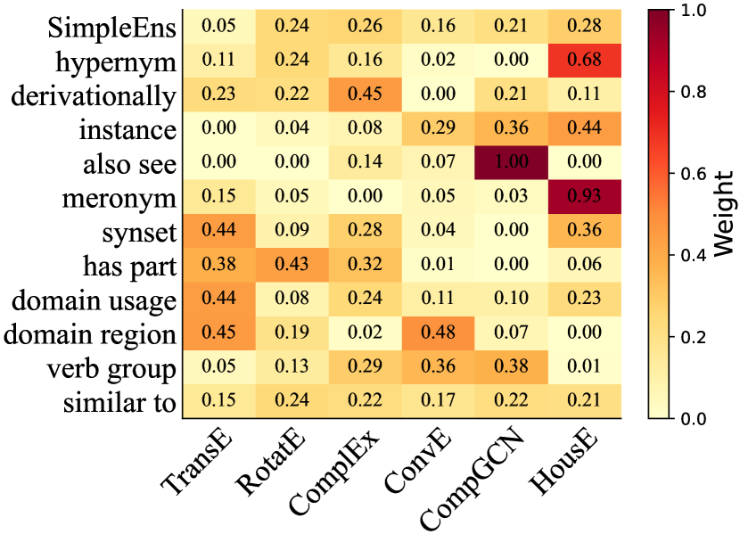
Figure 1: Ensemble weights of SimplEns and RelEns-DSC on the WN18RR dataset.

3.4 Efficiency Comparison

We compare the learning curves (highest MRR yet searched vs. running time) of SimpleEns, RelEns-Basic, and RelEns-DSC on NELL-995 in Figure 2 (the curves of other datasets are in Appendix C.1). The ensemble weights for all three methods are initialized as $\nicefrac{{1}}{{N}}$. We denote the number of parameter configurations for TPE to search as $Q$, and show the results of $Q=50$ and $Q=100$.

(a) $Q=50$

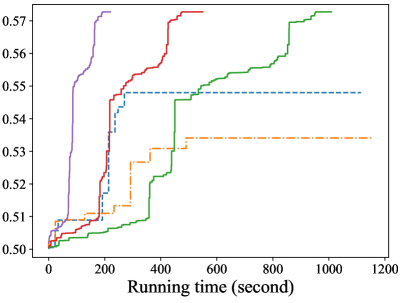
(b) $Q=100$

Figure 2: Learning curves of different ensemble methods on NELL-995. RelEns-DSC2/5 indicates the number of threads (2/5) used for parallel computing.

Based on the results, RelEns-Basic is much worse than SimpleEns, since the search complexity of RelEns-Basic increases exponentially. At the beginning of searching, RelEns-DSC is inferior to both SimpleEns and RelEns-Basic since it only searches the weights on a few relations, while others are unchanged. Over time, the performance of RelEns-DSC has improved significantly as more and more relations have found their optimal values. Increasing $Q$ from 50 to 100 did not lead to any improvement in the performance of SimpleEns and RelEns-Basic. However, RelEns-DSC was able to achieve better overall performance since increasing $Q$ allows the sub-problems to be more sufficiently solved with more iterations. In addition, RelEns-DSC can be benefited by parallel computing on the relation level, further improving efficiency.

3.5 Ablation Study

Table 3: Ablation study on WN18RR, FB15k-237 and NELL-995 dataset. “H@10” is short for Hit@10.

Dataset	WN18RR		FB15k-237		NELL-995
Model	MRR	H@10	MRR	H@10	MRR	H@10
Mean	.4963	.5746	.3572	.5457	.5412	.6622
Stacking	.4952	.5751	.3563	.5433	.5365	.6669
SimpleEns	.5121	.6021	.3621	.5525	.5416	.6601
MRR-Mean	.5143	.6028	.3645	.5547	.5460	.6604
RelEns-DSC	.5201	.6039	.3680	.5554	.5499	.6609

Table 3 shows the performance comparison of multiple variants of RelEns-DSC on the three benchmark datasets. Due to space limit, results of Hit@{1,3} and the implementation details of the variants are provided in Appendix B.2. The stacking method (Stacking), arithmetic mean method (Mean) and MRR-based weighted mean method (MRR-Mean) have poorer performance compared to RelEns-DSC. This indicates the importance of searching for ensemble weights with TPE technique. Stacking performs the worst since the non-differentiable metric MRR cannot directly optimized. In particular, considering relation-specific ensemble weights, RelEns-DSC can lead to better performance than the general ensemble methods.

4 Conclusion

This paper introduces a novel ensemble method, Relation-aware Ensemble with Divide-Search-Combine (RelEns-DSC) for KG embedding. The proposed RelEns-DSC learns relation-specific ensemble weights for different models and efficiently searches the weights using the divide-concur strategy. Empirical results demonstrate that our proposed method outperforms existing ensemble methods for KG embedding, in both effectiveness and efficiency.

Limitations.

The proposed method mainly addresses the ensemble problem for entity prediction tasks in knowledge graph completion. However, it does not effectively address the other graph learning tasks, such as entity/node classification, relation prediction, and graph classification. In addition, the significance of RelEns-DSC is under the case of multi-relational graphs like knowledge graph and heterogeneous graph, thus is not well adapted to homogeneous graph with single edge type.

Appendix A Supplementary Materials for the Method

A.1 Relation-wise Ensemble

An overview of the relation-wise ensemble problem is provided

in Figure 3. First, the dataset $\mathcal{D}$ is split into multiple sub-sets $\mathcal{D}^{1},\mathcal{D}^{2},\dots,\mathcal{D}^{R}$ according to the relations. For each sample $x^{r}_{j}$ from $\mathcal{D}^{r}$, the models $F_{1},F_{2},\dots,F_{N}$ output the scores and the ranking function $\Gamma(\cdot)$ provides ranking lists for the $C$ entities according to their scores. The relation-wise ensemble weights $\alpha^{r}_{1},\alpha^{r}_{2},\dots,\alpha^{r}_{N}$ re-weight the rank lists as the new scores $\bm{p}_{j}^{r}$ of $x^{r}_{j}$ and re-rank the new scores to evaluate the perfomance.

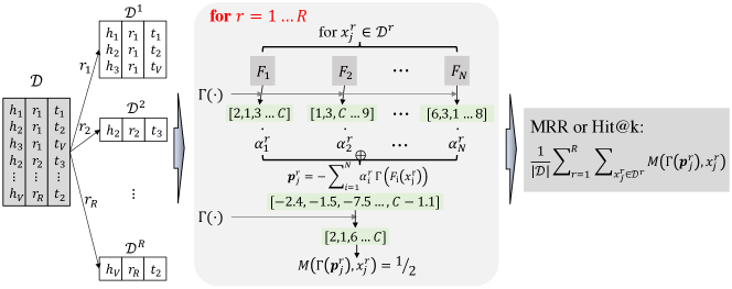
Figure 3: An overview of the relation-wise ensemble problem.

Two metrics are used in this paper: (i) Mean reciprocal ranking (MRR):

$$\text{MRR}=\frac{1}{2\left|\mathcal{D}\right|}\sum_{(h,r,t)\in\mathcal{D}}\big{(}\frac{1}{p_{h}}+\frac{1}{p_{t}}\big{)};$$

and (ii) Hit@$k$: ratio of ranks no larger than $k$, i.e.,

$$\text{Hit}@k=\frac{1}{2\left|\mathcal{D}\right|}\sum_{(h,r,t)\in\mathcal{D}}\big{(}\mathbb{I}(p_{h}\leq k)+\mathbb{I}(p_{t}\leq k)\big{)},$$

where $\mathbb{I}(a)=1$ if a is true, otherwise 0, $p_{h}$ is the rank of head entity $h$ in the head-prediction sub-task (the same for $p_{t}$ and $t$). The larger the MRR or Hit@$k$, the better is the embedding.

A.2 Relation Properties

In the main text, we claim that the different models work properly for different relations. In this part, we summarize the types of relations that different models can handle in Table 4.

Table 4: The pattern modeling and inference abilities of selected score functions.

Model	Symmetry	Antisymmetry	Inversion	Composition	Hierarchy
TransE	✗	✓	✓	✓	✗
RotatE	✓	✓	✓	✓	✗
HousE	✓	✓	✓	✓	✗
ComplEx	✓	✓	✓	✗	✓
ConvE	✓	✓	✗	✗	✓
CompGCN	✓	✓	✓	✗	✗

In addition, we show the performance of various base models for specific relations on WN18RR.

Among the total of eleven relations considered, we present the results based on the following four representative relations:

• membe_meronym: translational models such as TransE and RotatE exhibit the highest performance.

• synset_domain_topic_of: bilinear models like ComplEx achieve the best results.

• has_part: while traditional scoring functions perform well on this relation, neural network-based models such as ConvE and CompGCN exhibit suboptimal performance.

• verb_group: in contrast to has_part, neural network models such as ConvE and CompGCN perform better, whereas traditional scoring functions show inferior performance.

These results demonstrate that KG embedding models may specialize in different relations, leading to significant variation in their performance across relations.

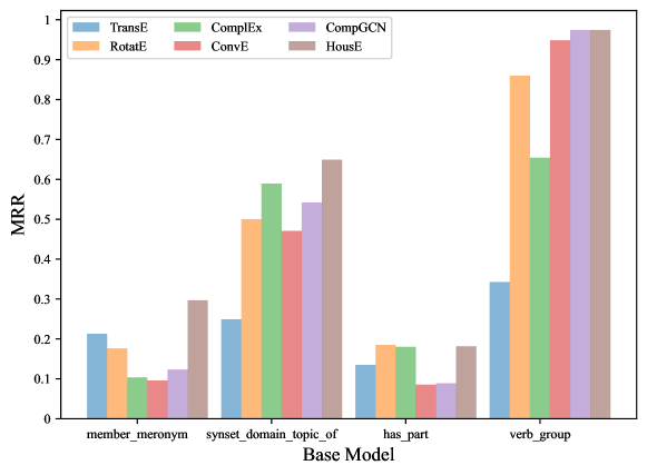
Figure 4: MRR of selected base models for specific relations on the WN18RR dataset.

Appendix B Supplementary Materials for the Experimental Settings

B.1 Statistics of Datasets

We use the following datasets for evaluation: (i) WN18RR is a link prediction dataset which is a subset of WordNet Dettmers et al. (2018); (ii) FB15k-237 contains triplets of knowledge base relationships and textual mentions of Freebase entity pairs Toutanova and Chen (2015); (iii) NELL-995 is a dataset built from the web via an intelligent agent called Never-Ending Language Learner that reads the web over time Xiong et al. (2017); (iv) ogbl-biokg is a KG, which was created using data from a large number of biomedical data repositories Hu et al. (2020); and (v) ogbl-wikikg2 is a KG extracted from the Wikidata knowledge base Hu et al. (2020). Statistics of these datasets are provided in Table 5.

Table 5: Statistics of the datasets.

Dataset	$|\mathcal{V}|$	$|\mathcal{R}|$	$|\mathcal{D}_{\text{tra}}|$	$|\mathcal{D}_{\text{val}}|$	$|\mathcal{D}_{\text{tst}}|$
WN18RR	40,943	11	86,835	3,034	3,134
FB15k-237	14,541	237	272,115	17,535	20,466
NELL-995	74,536	200	149,678	543	2,818
ogbl-biokg	93,773	51	4,762,678	162,886	162,870
ogbl-wikikg2	2,500,604	535	16,109,182	429,456	598,543

B.2 Hyperparameter Setting

We list the hyperparameters for base models in KGTuner Zhang et al. (2022b) on the WN18RR, FB15k-237 and NELL-995 datasets in Table 6 and Table 7.

Table 6: Hyperparameters for the WN18RR dataset.

HP/Model	ComplEx	ConvE	TransE	RotatE
# negative samples	32	512	128	2048
loss function	BCE_mean	BCE_adv	BCE_adv	BCE_adv
gamma	2.29	12.16	3.50	3.78
adv. weight	0.00	0.78	1.14	1.66
regularizer	NUC	DURA	FRO	FRO
reg. weight	$1.21\times 10^{-3}$	$9.79\times 10^{-3}$	$4.19\times 10^{-4}$	$5.13\times 10^{-8}$
dropout rate	0.28	0.02	0.00	0.00
optimizer	Adam	Adam	Adam	Adam
learning rate	$6.08\times 10^{-4}$	$6.88\times 10^{-4}$	$1.02\times 10^{-4}$	$1.24\times 10^{-3}$
initializer	x_uni	x_uni	norm	norm
batch size	1024	512	512	512
dimension size	2000	1000	1000	1000
inverse relation	False	False	False	False

Table 7: Hyperparameters for the FB15k-237 and NELL-996 datasets.

HP/Model	ComplEx	ConvE	TransE	RotatE
# negative samples	512	512	512	128
loss function	BCE_adv	BCE_sum	BCE_adv	BCE_adv
gamma	13.05	14.52	6.76	14.46
adv. weight	1.93	0.00	1.99	1.12
regularizer	DURA	DURA	FRO	NUC
reg. weight	$9.75\times 10^{-3}$	$6.42\times 10^{-3}$	$2.16\times 10^{-4}$	$2.99\times 10^{-4}$
dropout rate	0.22	0.07	0.02	0.01
optimizer	Adam	Adam	Adam	Adam
learning rate	$9.70\times 10^{-4}$	$2.09\times 10^{-4}$	$2.66\times 10^{-4}$	$5.89\times 10^{-4}$
initializer	uni	norm	x_norm	norm
batch size	1024	1024	512	1024
dimension size	2000	500	1000	2000
inverse relation	False	False	False	False

For CompGCN Vashishth et al. (2020), we use 200-dimensional embeddings for node and relation embeddings and apply the standard binary cross entropy loss with label smoothing. The number of GCN layers is 2, and the score function used in CompGCN is ConvE, the learning rate is set to 0.001, the batch size is 128, and the dropout rate is 0.1.

For HousE Li et al. (2022), we used the default hyperparameters specified in the original paper. Both node and relation embeddings were set to 800 dimensions. The learning rate was set to 0.0005, and the batch size was 1000.

For the top three methods on the OGB leaderboard , since their code has been officially made public by OGB, we used their code directly with their corresponding hyperparameters.

B.3 Details of Tree-structured Parzen Estimator (TPE)

The TPE (Tree-structured Parzen Estimator) algorithm is a Bayesian optimization Snoek et al. (2012) method that aims to efficiently optimize black-box functions with a limited budget of function evaluations. It was introduced by Bergstra et al. (2011) as a part of the Hyperopt framework Bergstra et al. (2015), which focuses on hyperparameter optimization. Bayesian optimization is a sequential model-based optimization technique that leverages prior knowledge and data to intelligently search for the optimal solution. It uses a probabilistic surrogate model, typically a Gaussian process or a tree-based model, to model the unknown objective function. This model is iteratively updated as new observations are made, providing an estimate of the function’s behavior and uncertainty.

The TPE algorithm improves upon traditional Bayesian optimization by employing a novel method for modeling and sampling from the posterior distribution of the objective function. It uses a tree-structured Parzen estimator to model the distribution of good and bad parameter configurations. The algorithm maintains two density functions: $p\left(x|y\right)=\ell(x){\text{ if }y<y^{\ast}}$ otherwise $p\left(x|y\right)=g(x)$, where $\ell(x)$ is the density formed by using observations $\{x^{(i)}\}$ from past evaluations, such that the corresponding loss (i.e., the performance metric for the model) is less than some threshold $y^{\ast}$ that lead to good results, and $g(x)$ is the density formed by using the remaining observations that lead to bad results.

At each iteration, the TPE algorithm samples promising configurations from the good density and less promising configurations from the bad density. The algorithm balances the exploration-exploitation trade-off by dividing the sampled configurations into two groups based on their relative performance. The better-performing configurations are used to update the density function for good configurations, while the less successful ones update the density function for bad configurations. This process aims to guide the search towards promising regions of the parameter space. By iteratively updating the density functions and adaptively sampling configurations, the TPE algorithm efficiently explores the parameter space, gradually converging towards the optimal solution. It has been shown to be effective in hyperparameter optimization for machine learning models and other optimization tasks.

Overall, the TPE algorithm, as a Bayesian optimization method, offers a principled and efficient approach for optimizing black-box functions with limited resources, making it particularly useful in scenarios where function evaluations are time-consuming or costly.

Appendix C Supplementary Materials for Experimental Results

C.1 Full Results of Learning Curves

We provide the learning curves on WN18RR, FB15k-237 and NELL-995 datasets in this part. Figure 5 confirms that the observations in Section 3.4 are consistent with the results presented here. While RelEns-Basic exhibits a superior modeling ability compared to SimpleEns by learning relation-specific weights, enabling different models to specialize in different relations. However, the search complexity of RelEns-Basic increases exponentially with the number of relations.

• On WN18RR with only 11 relations, RelEns-Basic can slightly outperform SimpleEns since the complexity is not increased much and the relation-wise ensemble problem can have better performance than the general ensemble problem.

• Nevertheless, on datasets containing hundreds of relations such as FB15k-237 and NELL-995 RelEns-Basic exhibits significantly poorer performance compared to SimpleEns due to high sampling complexity in the relation-wise ensemble problem.

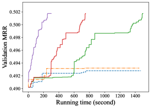
(a) WN18RR with $Q=50$

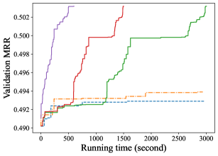
(b) WN18RR with $Q=100$

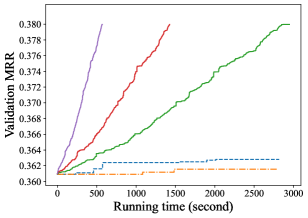
(c) FB15k-237 with $Q=50$

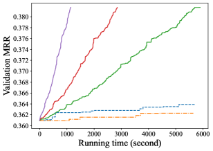
(d) FB15k-237 with $Q=100$

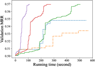
(e) NELL-995 with $Q=50$

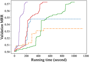
(f) NELL-995 with $Q=100$

(g) ogbl-wikikg2 with $Q=50$

(h) ogbl-wikikg2 with $Q=100$

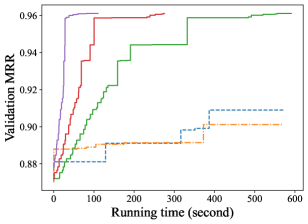
(i) ogbl-biokg with $Q=50$

(j) ogbl-biokg with $Q=100$

Figure 5: Learning curves of different ensemble methods. RelEns-DSC2/5 indicates the number of threads used for parallel computing.

C.2 Ablation Study on Ensemble methods

All the variants use the same way to ensemble predictions of base models. The same as mentioned in Section 2.1, we use the ensemble weights on rankings of base models as the ensemble score, i.e., $\bm{p}_{j}^{r}=-\sum\nolimits_{i=1}^{N}\alpha_{i}^{r}\Gamma\big{(}F_{i}(x_{j}^{r})\big{)}$. The implementation details of the ensemble variants are provided as follows:

• Mean: This is the most basic ensemble method which directly takes the arithmetic mean of the predictions made by each individual model.

• Stacking Wolpert (1992): The stacking ensemble variant is a more sophisticated approach that involves training a meta-model to learn how to combine the predictions of multiple base models. Specifically, the rank lists outputted by the base models are used as features to train the meta-model. Here, we use a logistic regression model implemented by scikit-learn Pedregosa et al. (2011) as the meta-model, with a maximum iteration of 300. Since the ranking metrics on the validation data is non-differentiable, we use the same loss function during training on the validation data to optimize the parameters of meta-model.

• SimpleEns: This variant is a degenerated problem of (1) by setting identical ensemble weights of different relations on a single mode, i.e., $\alpha_{i}^{1}=\alpha_{i}^{2}=\cdots=\alpha_{i}^{R}$ for $i=1,\dots,N$. In order to keep consistent with RelEns-Basic and RelEns-DSC, these weights are searched by optimizing (1) with TPE technique.

• MRR-Mean: The MRR-Mean variant incorporates the Mean Reciprocal Rank (MRR) of the base model as a weighting factor. In contrast to the Mean variant, it assigns proportionally greater weight to the superior individual base model.

We conducted an ablation study on the WN18RR, FB15k-237, and NELL-995 datasets, and the results are shown in Table 8. MRR can provide a general indication of the importance of different models, but higher MRR does not always correlate with higher model importance due to the crucial role of diversity among the base models in the ensemble strategy. Additionally, MRR-weight may not be optimal weights, necessitating further weight searches to enhance performance. The results consistently demonstrate the superiority of searched methods (RelEns-DSC) over MRR-weighted methods (MRR-Mean).

Table 8: Comparison of ensemble methods on WN18RR, FB15k-237 and NELL-995 datasets.

Dataset	WN18RR				FB15k-237				NELL-995
Model	MRR	Hit@1	Hit@3	Hit@10	MRR	Hit@1	Hit@3	Hit@10	MRR	Hit@1	Hit@3	Hit@10
Mean	0.4963	0.4531	0.5175	0.5746	0.3572	0.2643	0.3918	0.5457	0.5412	0.4661	0.5823	0.6622
Stacking	0.4952	0.4518	0.5169	0.5751	0.3563	0.2639	0.3921	0.5433	0.5365	0.4637	0.5851	0.6669
SimpleEns	0.5121	0.4670	0.5289	0.6021	0.3621	0.2683	0.3977	0.5525	0.5416	0.4758	0.5823	0.6601
MRR-Mean	0.5143	0.4697	0.5311	0.6028	0.3645	0.2702	0.3993	0.5547	0.5460	0.4732	0.5834	0.6604
RelEns-DSC	0.5201	0.4770	0.5375	0.6039	0.3680	0.2746	0.4046	0.5554	0.5499	0.4823	0.5901	0.6609

References

- Bergstra et al. (2011) James Bergstra, Rémi Bardenet, Yoshua Bengio, and Balázs Kégl. 2011. Algorithms for hyper-parameter optimization. In NIPS, pages 2546–2554.
- Bergstra et al. (2015) James Bergstra, Brent Komer, Chris Eliasmith, Dan Yamins, and David D Cox. 2015. Hyperopt: A python library for model selection and hyperparameter optimization. Comput. Sci. Discov., 8(1):014008.
- Bordes et al. (2013) Antoine Bordes, Nicolas Usunier, Alberto Garcia-Duran, Jason Weston, and Oksana Yakhnenko. 2013. Translating embeddings for modeling multi-relational data. In NeurIPS, pages 2787–2795.
- Breiman (1996) Leo Breiman. 1996. Bagging predictors. Machine Learning, 24:123–140.
- Chen et al. (2021) Yihong Chen, Pasquale Minervini, Sebastian Riedel, and Pontus Stenetorp. 2021. Relation prediction as an auxiliary training objective for improving multi-relational graph representations. arXiv:2110.02834.
- Dettmers et al. (2018) Tim Dettmers, Pasquale Minervini, Pontus Stenetorp, and Sebastian Riedel. 2018. Convolutional 2D knowledge graph embeddings. In AAAI, volume 32.
- Dietterich (2000) Thomas G Dietterich. 2000. Ensemble methods in machine learning. In MCS, pages 1–15. Springer.
- Hu et al. (2020) Weihua Hu, Matthias Fey, Marinka Zitnik, Yuxiao Dong, Hongyu Ren, Bowen Liu, Michele Catasta, and Jure Leskovec. 2020. Open graph benchmark: Datasets for machine learning on graphs. NeurIPS.
- Ji et al. (2021) Shaoxiong Ji, Shirui Pan, Erik Cambria, Pekka Marttinen, and S Yu Philip. 2021. A survey on knowledge graphs: Representation, acquisition, and applications. IEEE transactions on neural networks and learning systems, 33(2):494–514.
- Köppen (2000) Mario Köppen. 2000. The curse of dimensionality. In 5th Online World Conference on Soft Computing in Industrial Applications, volume 1, pages 4–8.
- Krompaß and Tresp (2015) Denis Krompaß and Volker Tresp. 2015. Ensemble solutions for link-prediction in knowledge graphs. In PKDD ECML 2nd Workshop on Linked Data for Knowledge Discovery.
- (12) Hongzhu Li, Xiangrui Gao, Linhui Feng, Yafeng Deng, and Yuhui Yin. Stargraph: Knowledge representation learning based on incomplete two-hop subgraph. Technical report.
- Li et al. (2022) Rui Li, Jianan Zhao, Chaozhuo Li, Di He, Yiqi Wang, Yuming Liu, Hao Sun, Senzhang Wang, Weiwei Deng, Yanming Shen, et al. 2022. House: Knowledge graph embedding with householder parameterization. In ICML, pages 13209–13224. PMLR.
- Pedregosa et al. (2011) Fabian Pedregosa, Gaël Varoquaux, Alexandre Gramfort, Vincent Michel, Bertrand Thirion, Olivier Grisel, Mathieu Blondel, Peter Prettenhofer, Ron Weiss, Vincent Dubourg, et al. 2011. Scikit-learn: Machine learning in python. the Journal of machine Learning research, 12:2825–2830.
- Rivas-Barragan et al. (2022) Daniel Rivas-Barragan, Daniel Domingo-Fernández, Yojana Gadiya, and David Healey. 2022. Ensembles of knowledge graph embedding models improve predictions for drug discovery. Briefings in Bioinformatics, 23(6):bbac481.
- Snoek et al. (2012) Jasper Snoek, Hugo Larochelle, and Ryan P Adams. 2012. Practical bayesian optimization of machine learning algorithms. NIPS, 25.
- Sun et al. (2019) Zhiqing Sun, Zhi-Hong Deng, Jian-Yun Nie, and Jian Tang. 2019. Rotate: Knowledge graph embedding by relational rotation in complex space. In ICLR.
- Toutanova and Chen (2015) Kristina Toutanova and Danqi Chen. 2015. Observed versus latent features for knowledge base and text inference. In CVSC, pages 57–66.
- Trouillon et al. (2017) Théo Trouillon, Christopher R Dance, Johannes Welbl, Sebastian Riedel, Éric Gaussier, and Guillaume Bouchard. 2017. Knowledge graph completion via complex tensor factorization. JMLR, 18(1):4735–4772.
- Vashishth et al. (2020) Shikhar Vashishth, Soumya Sanyal, Vikram Nitin, and Partha Talukdar. 2020. Composition-based multi-relational graph convolutional networks. ICLR.
- Wang et al. (2022a) Baoxin Wang, Qingye Meng, Ziyue Wang, Dayong Wu, Wanxiang Che, Shijin Wang, Zhigang Chen, and Cong Liu. 2022a. InterHT: Knowledge graph embeddings by interaction between head and tail entities. arXiv:2202.04897.
- Wang et al. (2017) Quan Wang, Zhendong Mao, Bin Wang, and Li Guo. 2017. Knowledge graph embedding: A survey of approaches and applications. TKDE, 29(12):2724–2743.
- Wang et al. (2022b) Yinquan Wang, Yao Chen, Zhe Zhang, and Tian Wang. 2022b. A probabilistic ensemble approach for knowledge graph embedding. Neurocomputing, 500:1041–1051.
- Wolpert (1992) David H Wolpert. 1992. Stacked generalization. Neural Networks, 5(2):241–259.
- Xiong et al. (2017) Wenhan Xiong, Thien Hoang, and William Yang Wang. 2017. DeepPath: A reinforcement learning method for knowledge graph reasoning. arXiv:1707.06690.
- Yao et al. (2023) Liang Yao, Jiazhen Peng, Qiang Liu, Hongyun Cai, Shenggong Ji, Feng He, and Xu Cheng. 2023. Technical report for OGB link property prediction: ogbl-wikikg2.
- Yu et al. (2022) Long Yu, Zhicong Luo, Huanyong Liu, Deng Lin, Hongzhu Li, and Yafeng Deng. 2022. TripleRE: Knowledge graph embeddings via tripled relation vectors. arXiv:2209.08271.
- Zhang et al. (2022a) Yongqi Zhang, Quanming Yao, and James T Kwok. 2022a. Bilinear scoring function search for knowledge graph learning. TPAMI.
- Zhang et al. (2022b) Yongqi Zhang, Zhanke Zhou, Quanming Yao, and Yong Li. 2022b. KGTuner: Efficient hyper-parameter search for knowledge graph learning. In ACL.