Community Membership Hiding as Counterfactual Graph Search via Deep Reinforcement Learning

Abstract.

Community detection techniques are useful tools for social media platforms to discover tightly connected groups of users who share common interests. However, this functionality often comes at the expense of potentially exposing individuals to privacy breaches by inadvertently revealing their tastes or preferences. Therefore, some users may wish to safeguard their anonymity and opt out of community detection for various reasons, such as affiliation with political or religious organizations.
In this study, we address the challenge of community membership hiding, which involves strategically altering the structural properties of a network graph to prevent one or more nodes from being identified by a given community detection algorithm. We tackle this problem by formulating it as a constrained counterfactual graph objective, and we solve it via deep reinforcement learning. We validate the effectiveness of our method through two distinct tasks: node and community deception. Extensive experiments show that our approach overall outperforms existing baselines in both tasks.

1. Introduction

In the ever-expanding landscape of interconnected entities, such as social networks, online platforms, and collaborative ecosystems, the identification of coherent communities plays a pivotal role in understanding complex network graph structures (Fortunato, 2010). The task of identifying these communities is typically accomplished by running community detection algorithms on the network graphs, which allows the unveiling of hidden patterns and relationships among nodes within these structures. These algorithms effectively group entities, users, or objects based on shared characteristics or interactions, shedding light on the underlying organization and dynamics of the network.

The successful detection of communities in complex network graphs is useful in several application domains (Karataş and Şahin, 2018). For instance, the insights gained from accurately identifying communities can significantly impact business strategies, leading to better monetization opportunities through targeted advertising. By understanding the specific interests and behaviors of community members, businesses can provide better service solutions and tailor advertisements that are more relevant to their customer segments, resulting in higher engagement and increased revenue (Mosadegh and Behboudi, 2011).

However, while community detection algorithms offer immense benefits, they also raise concerns regarding individual privacy and data protection. In some cases, certain nodes within the network might prefer to remain undetected as part of any specific community. These nodes could belong to sensitive or private groups (e.g., political organizations or religious associations) or may simply wish to retain their anonymity for personal reasons. Anyway, the right to opt out of community detection becomes crucial to strike a balance between preserving privacy and maximizing the utility of these algorithms.

Motivated by the need above, in this paper, we address the intriguing challenge of community membership hiding.

Taking inspiration from the concept of counterfactual reasoning (Tolomei et al., 2017; Tolomei and Silvestri, 2021), specifically for graph data (Lucic et al., 2022), our objective is to offer users personalized recommendations to preserve their anonymity from community detection. We effectively guide them in adjusting their connections so that they cannot be identified as members of a given community. For instance, we might suggest to a hypothetical user of a social network, “If you unfollow users X and Y, you will no longer be recognized as a member of community Z.”

The core challenge of this problem lies in determining how to strategically modify the structural properties of a network graph, effectively excluding one or more nodes from being identified by a given community detection algorithm. To the best of our knowledge, we are the first to formulate the community membership hiding problem as a constrained counterfactual graph objective. Furthermore, inspired by (Chen et al., 2022), we cast this problem into a Markov decision process (MDP) framework and we propose a deep reinforcement learning (DRL) approach to solve it.

Our method works as follows. We start with a graph and a set of communities identified by a specific community detection algorithm whose inner logic remains unknown or undisclosed. When given a target node within a community, our objective is to find the optimal structural adjustment of the target node’s neighborhood. This adjustment should enable the target node to remain concealed when the same community detection algorithm is reapplied to the modified graph. We refer to this primary task as node deception, and we consider it successful when a predefined similarity threshold between the original community and the new community containing the target node is met. In addition to this, we define a community deception task – already investigated in the literature (Fionda and Pirrò, 2018) – whose goal is to mask all the nodes of a given community.

We validate our approach on three real-world datasets, and we demonstrate that it outperforms existing baselines using standard quality metrics both on node and community deception tasks. Furthermore, unlike their competitors, our method maintains its effectiveness even when used in conjunction with a community detection algorithm that was not seen during the training phase.

The main contributions of our work are summarized below.

• We formulate the community membership hiding problem as a constrained counterfactual graph objective.

• We cast this problem within an MDP framework and solved it via DRL.

• We utilize a graph neural network (GNN) representation to capture the structural complexity of the input graph, which in turn is used by the DRL agent to make its decisions.

• We validate the performance of our method in comparison with existing baselines using standard quality metrics both on node and community deception tasks.

• We publicly release both the source code and the data utilized in this study to encourage reproducibility.

The remainder of this paper is structured as follows. In Section 2, we review related work. Section 3 contains background and preliminaries. We present our problem formulation in Section 4. In Section 5, we describe our method, which we validate through extensive experiments in Section 6. Section 7 discusses the potential ethical impact of our method. Finally, we conclude in Section 8.

2. Related Work

2.1. Community Detection

Community detection algorithms are essential tools in network analysis, aiming to uncover densely connected groups of nodes within a graph. Their applications span various domains, including social network analysis, biology, and economics.

These algorithms can be broadly categorized into two types: non-overlapping and overlapping community detection. Non-overlapping community detection assigns each node to a single community, employing various techniques such as Modularity Optimization (Blondel et al., 2008), Spectrum Analysis (Ruan et al., 2012), Random Walk (Pons and Latapy, 2005), or Label Propagation (Raghavan et al., 2007). On the other hand, overlapping community detection seeks to better represent real-world networks where nodes can belong to multiple communities. Mature methods have been developed for this purpose, including NISE (Neighborhood-Inflated Seed Expansion) (Whang et al., 2015) and techniques centered around minimizing the Hamiltonian of the Potts model (Ronhovde and Nussinov, 2009). For a more comprehensive overview, we recommend consulting the work by Jin et al. (2021)

2.2. Community Deception

Community deception is closely related to the community membership hiding problem we investigate in this work. In fact, community deception can be seen as a specialization of community membership hiding, where the objective is to hide an entire community from community detection algorithms. Community deception can serve various purposes, such as preserving individuals’ anonymity in online monitoring scenarios, like social networks, or aiding public safety by identifying online criminal activities. However, there is also a darker side to these techniques, as malicious actors can exploit them to evade detection algorithms and operate covertly, potentially violating the law.

Several techniques exist for hiding communities, including those based on the concept of Modularity. Notable examples in this category include the algorithm proposed by Nagaraja (2010), one of the pioneering approaches in this field, the DICE algorithm introduced by Waniek et al. (2018), and the algorithm developed by Fionda and Pirrò (2018). Other deception techniques are founded on the idea of Safeness, as defined by Fionda and Pirrò (2018) and further explored by Chen et al. (2021), as well as the concept of Permanence as developed by Mittal et al. (2021). For a more exhaustive summary of these methods, we suggest referring to (Kalaichelvi and Easwarakumar, 2022).

3. Background and Preliminaries

In this section, we will briefly review the definition of the well-known community detection problem. Afterward, we will utilize this definition as the foundation to provide our formulation of the community membership hiding problem.

Let $\mathcal{G}=(\mathcal{V},\mathcal{E})$ be an arbitrary (directed) graph, where $\mathcal{V}$ is a set of $n$ nodes ($|\mathcal{V}|=n$), and $\mathcal{E}\subseteq\mathcal{V}\times\mathcal{V}$ is a set of $m$ edges ($|\mathcal{E}|=m$). Optionally, an additional set of $p$ node attributes may also be present. In such cases, each node $u\in\mathcal{V}$ is associated with a corresponding $p$-dimensional real-valued feature vector $\bm{x}_{u}\in\mathbb{R}^{p}$. Furthermore, the underlying link structure of $\mathcal{G}$ is represented using a binary adjacency matrix $\bm{A}\in\{0,1\}^{n\times n}$, where $\bm{A}_{u,v}=1$ if and only if the edge $(u,v)\in\mathcal{E}$, and it is $0$ otherwise.

The community detection problem aims to identify clusters of nodes within a graph, called communities. Due to the intricate nature of the concept and its reliance on contextual factors, establishing a universally accepted definition for a “community” is challenging. Intuitively, communities exhibit strong intra-cluster connections and relatively weaker inter-cluster connections (Zhao et al., 2012).

More formally, in this work, we adhere to the definition widely used in the literature (Fionda and Pirrò, 2018; Kumari et al., 2021; Liu et al., 2019; Mittal et al., 2021), and we consider a function $f(\cdot)$ that takes a graph as input and generates a partition of its nodes $\mathcal{V}$ into a set of non-empty, non-overlapping, communities $\{\mathcal{C}_{1},\ldots,\mathcal{C}_{k}\}$ as output, i.e., $f(\mathcal{G})=\{\mathcal{C}_{1},\ldots,\mathcal{C}_{k}\}$, where $k$ is usually unknown. Within this framework, every node $u\in\mathcal{V}$ is assigned to exactly one community. This assignment can be captured using a $k$-dimensional stochastic vector $\bm{c}_{u}$, where $c_{u,i}=P(u\in\mathcal{C}_{i})$ measures the probability that node $u$ belongs to community $\mathcal{C}_{i}$, and $\sum_{i=1}^{k}c_{u,i}=1$. Eventually, we use the notation $i^{*}_{u}=\operatorname*{arg\,max}_{i}(c_{u,i})$ to represent the index of the community to which a specific node $u$ belongs to based on the outcome of $f(\mathcal{G})$. Note that in the case of hard node partitioning, there exists only one non-zero entry in the vector $\bm{c}_{u}$, which evaluates to $1$. However, this framework can be extended to scenarios with overlapping communities, where each node can belong to multiple clusters, resulting in more than one non-zero entry in $\bm{c}_{u}$. We leave the exploration of overlapping communities for future work.

Typically, community detection methods operate by maximizing a specific score that measures the intra-community cohesiveness (e.g., Modularity (Newman, 2006b)). However, this usually translates into solving NP-hard optimization problems. Hence, some convenient approximations have been proposed in the literature to realize $f(\cdot)$ in practice, e.g., Louvain (Blondel et al., 2008), WalkTrap (Pons and Latapy, 2005), Greedy (Brandes et al., 2008), InfoMap (Campan et al., 2015), Label Propagation (Raghavan et al., 2007), Leading Eigenvectors (Newman, 2006a), Edge-Betweeness (Girvan and Newman, 2002), SpinGlass (Reichardt and Bornholdt, 2006). Anyway, the rationale behind how communities are found is irrelevant to our task, and, hereinafter, we will treat the community detection technique $f(\cdot)$ as a “black box”.

4. Community Membership Hiding

In a nutshell, community membership hiding aims to enable a target node within a graph to elude being recognized as a member of a particular node cluster, as determined by a community detection algorithm. This objective is accomplished by granting the node in question the ability to strategically modify its connections with other nodes. Therefore, our primary focus is on making changes to the graph’s structure, represented by the adjacency matrix. While altering node features holds potential interest, that aspect is reserved for future exploration. We depict our approach in Fig. 1.

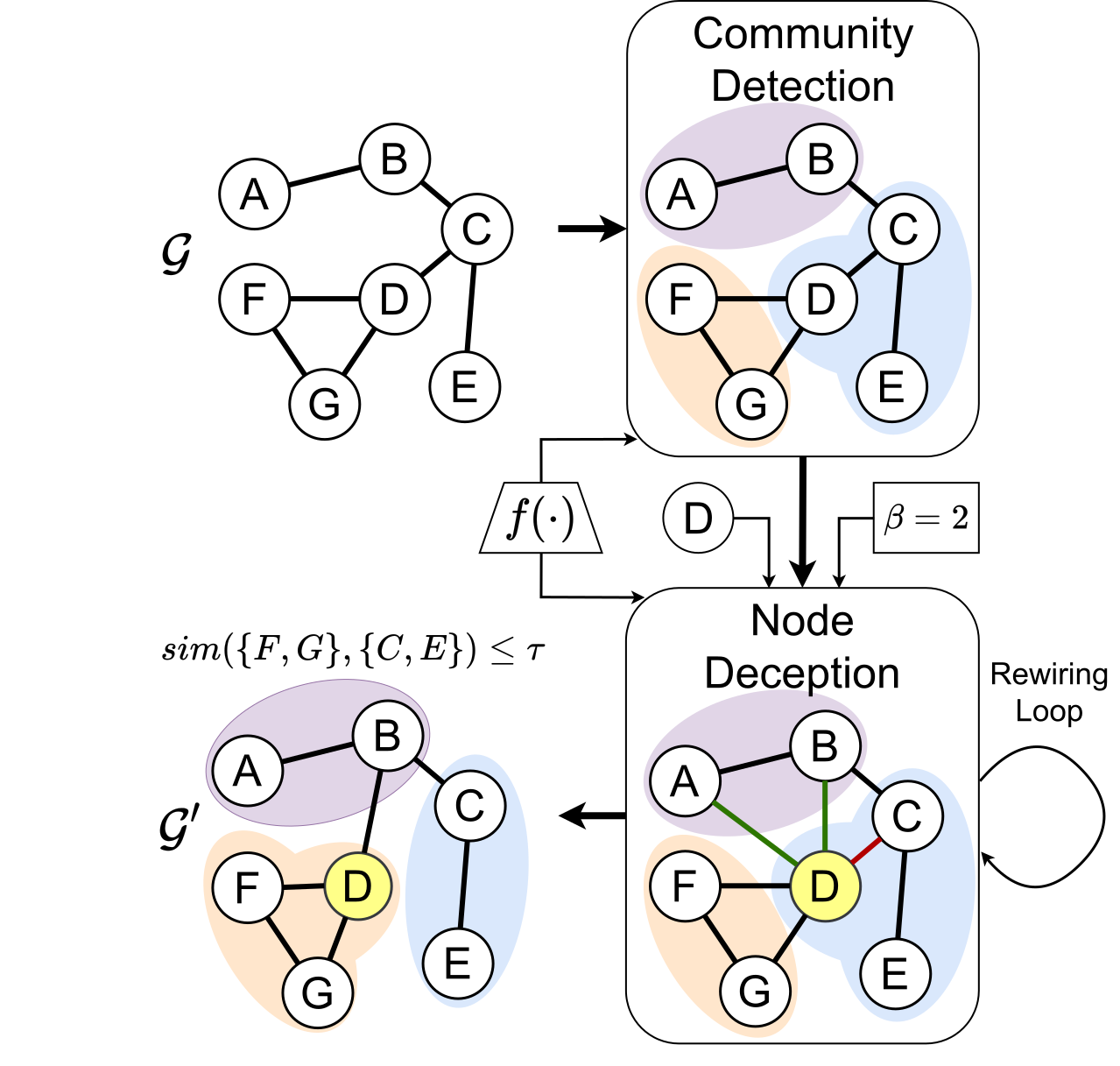
Figure 1. Given a graph $\mathcal{G}$, a node $u$ (in this case $u=D$), a budget of actions $\beta$, and the set of communities identified by the community detection algorithm $f(\cdot)$ (including the community $\mathcal{C}_{i}$ to which the node belongs), community membership hiding consists of adding inter-community edges $\mathcal{E}_{u,i}^{+}$ (green edges), or removing intra-community edges $\mathcal{E}_{u,i}^{-}$ (red edge), so that the value returned by the similarity function $sim(\cdot,\cdot)$, between the new community to which the node belongs after rewiring, and the original one, is lower than the $\tau$ constraint.

4.1. Problem Formulation

Let $\mathcal{G}=(\mathcal{V},\mathcal{E})$ be a graph and $f(\mathcal{G})=\{\mathcal{C}_{1},\ldots,\mathcal{C}_{k}\}$ denote the community arrangement derived from applying a detection algorithm $f(\cdot)$ to $\mathcal{G}$. Furthermore, suppose that $f$ has identified node $u\in\mathcal{V}$ as a member of the community $\mathcal{C}_{i}\in f(\mathcal{G})$ – i.e., $i^{*}_{u}=i$ – denoted as $u\in\mathcal{C}_{i}$. The aim of community membership hiding is to formulate a function $h_{\bm{\theta}}(\cdot)$, parametrized by $\bm{\theta}$, that takes as input the initial graph $\mathcal{G}$ and produces as output a new graph $h_{\bm{\theta}}(\mathcal{G})=\mathcal{G^{\prime}}=(\mathcal{V},\mathcal{E^{\prime}})$. Among all the possible graphs, we seek the one which, when input to the community detection algorithm $f$, disassociates a target node $u$ from its original community $\mathcal{C}_{i}$. To achieve that goal, suppose that the target node $u$ is associated with a new community $\mathcal{C}^{\prime}_{i}\in f(\mathcal{G}^{\prime})$. Hence, we can define the objective of community membership hiding by establishing a threshold for the similarity between $\mathcal{C}^{\prime}_{i}$ and $\mathcal{C}_{i}$, excluding the target node $u$, which, by definition, belongs to both communities. In other words, we set a condition: $sim(\mathcal{C}_{i}-\{u\},\mathcal{C}^{\prime}_{i}-\{u\})\leq\tau$, where $\tau\in[0,1]$.

Several similarity measures can be used to measure $sim(\cdot,\cdot)$ depending on the application domain, e.g., the overlap coefficient (a.k.a. Szymkiewicz–Simpson coefficient) (M.K and K, 2016), the Jaccard coefficient (Jaccard, 1912), and the Sørensen-Dice coefficient (Dice, 1945).

Setting $\tau=0$ represents the most stringent scenario, where we require zero overlaps between $\mathcal{C}^{\prime}_{i}$ and $\mathcal{C}_{i}$, except for the node $u$ itself. At the other extreme, when $\tau=1$, we adopt a more tolerant strategy, allowing for maximum overlap between $\mathcal{C}^{\prime}_{i}$ and $\mathcal{C}_{i}$. However, it is important to note that except for the overlap coefficient, which can yield a value of $1$ even if one community is a subset of the other, the Jaccard and Sørensen-Dice coefficients yield a value of $1$ only when the two communities are identical. In practice, setting $\tau=1$ may lead to the undesired outcome of $\mathcal{C}^{\prime}_{i}$ being equal to $\mathcal{C}_{i}$, thus contradicting the primary goal of community membership hiding. Therefore, it is common to let $\tau\in[0,1)$ to avoid this scenario.

Moreover, it is essential to emphasize that executing $f$ on $\mathcal{G}^{\prime}$ instead of the original $\mathcal{G}$ could potentially influence $(i)$ the community affiliations of nodes beyond the selected target, $u$, and $(ii)$ the eventual count of recognized communities (i.e., $|f(\mathcal{G}^{\prime})|=k^{\prime}\neq k=|f(\mathcal{G})|$), providing that $f$ does not need this number fixed apriori as one of its inputs. Therefore, community membership hiding must strike a balance between two conflicting goals. On the one hand, the target node $u$ must be successfully elided from the original community $\mathcal{C}_{i}$; on the other hand, the cost of such an operation – i.e., the “distance” between $\mathcal{G}$ and $\mathcal{G}^{\prime}$, and between $f(\mathcal{G})$ and $f(\mathcal{G}^{\prime})$ – must be as small as possible.

Overall, we can define the following loss function associated with the community membership hiding task:

(1) $$\mathcal{L}(h_{\bm{\theta}};\mathcal{G},f,u)=\ell_{\text{decept}}(\mathcal{G},h_{\bm{\theta}}(\mathcal{G});f,u)+\lambda\ell_{\text{dist}}(\mathcal{G},h_{\bm{\theta}}(\mathcal{G});f).$$

The first component ($\ell_{\text{decept}}$) penalizes when the goal is not satisfied. Let $\Gamma$ be the set of input graphs which do not meet the membership hiding objective, i.e., those which retain node $u$ as part of the community $\mathcal{C}_{i}$. More formally, let $\mathcal{\widetilde{C}}_{i}$ be the community to which node $u$ is assigned when $f$ is applied to the input graph $\widetilde{\mathcal{G}}$. We define $\Gamma=\{\widetilde{\mathcal{G}}~{}|~{}sim(\mathcal{C}_{i}-\{u\},\mathcal{\widetilde{C}}_{i}-\{u\})>\tau\}$. Thus, we can compute $\ell_{\text{decept}}$ as follows:

(2) $$\ell_{\text{decept}}(\mathcal{G},h_{\bm{\theta}}(\mathcal{G});f)=\mathbbm{1}_{\Gamma}(h_{\bm{\theta}}(\mathcal{G})),$$

where $\mathbbm{1}_{\Gamma}(h_{\bm{\theta}}(\mathcal{G}))$ is the well-known $0$-$1$ indicator function, which evaluates to $1$ if $h_{\bm{\theta}}(\mathcal{G})\in\Gamma$, or $0$ otherwise.

The second component, denoted as $\ell_{\text{dist}}$, is a composite function designed to assess the overall dissimilarity between two graphs and their respective communities found by $f$. This function serves the dual purpose of $(i)$ discouraging the new graph $h_{\bm{\theta}}(\mathcal{G})$ from diverging significantly from the original graph $\mathcal{G}$ and $(ii)$ preventing the new community structure $f(h_{\bm{\theta}}(\mathcal{G}))$ from differing substantially from the prior community structure $f(\mathcal{G})$.

4.2. Counterfactual Graph Objective

Given the target community $\mathcal{C}_{i}$, from which we want to exclude node $u$, we can classify the remaining nodes $\mathcal{V}-\{u\}$ of $\mathcal{G}$ into two categories: nodes that are inside the same community $\mathcal{C}_{i}$ as $u$ and nodes that belong to a different community from $u$. This categorization helps us define which edges the target node $u$ can control and, thus, directly manipulate under the assumption that $\mathcal{G}$ is a directed graph. Specifically, following (Fionda and Pirrò, 2018), we assume that $u$ can $(i)$ remove existing outgoing edges to nodes that are inside $u$’s community $(ii)$ add new outgoing edges to nodes that are outside $u$’s community. We intentionally exclude two possible actions: $(iii)$ removing outgoing links to outside-community nodes and $(iv)$ adding outgoing links to inside-community nodes. Two primary reasons drive this choice. On the one hand, allowing $(iii)$ could isolate $u$ and its original community $\mathcal{C}_{i}$ further. On the other hand, allowing $(iv)$ would enhance connectivity between $u$ and other nodes in $\mathcal{C}_{i}$. Both events contradict the goal of community membership hiding.

Overall, we can define the set of candidate edges to remove ($\mathcal{E}_{u,i}^{-}$) and to add ($\mathcal{E}_{u,i}^{+}$) as follows.

$$\mathcal{E}_{u,i}^{-} =\{(u,v)~{}|~{}u,v\in\mathcal{C}_{i}\wedge(u,v)\in\mathcal{E}\},$$

$$\mathcal{E}_{u,i}^{+} =\{(u,v)~{}|~{}u\in\mathcal{C}_{i},v\notin\mathcal{C}_{i}\wedge(u,v)\notin\mathcal{E}\}.$$

If we suppose the target node $u$ has a fixed budget $\beta>0$, we can find the optimal model $h^{*}=h_{\bm{\theta}^{*}}$ as the one whose parameters $\bm{\theta}^{*}$ minimize Eq. (1), i.e., by solving the following constrained objective:

(3) $$\begin{split}\bm{\theta}^{*}&=\underset{\bm{\theta}}{\text{arg min}}\bigg{\{}\mathcal{L}(h_{\bm{\theta}};\mathcal{G},f,u)\bigg{\}}\\ &\text{subjetc to: }|\mathcal{B}_{u,i}|\leq\beta,\end{split}$$

where $\mathcal{B}_{u,i}\subseteq\mathcal{E}_{u,i}^{-}\cup\mathcal{E}_{u,i}^{+}$ is the set of graph edge modifications selected from the candidates.

Note that Eq. (3) resembles the optimization task to find the best counterfactual graph $\mathcal{G}^{*}=h^{*}(\mathcal{G})$ that, when fed back into $f$, changes its output to hide the target node $u$ from its community.

4.3. Markov Decision Process

The community membership hiding problem defined in Eq. (3) requires minimizing a discrete, non-differentiable loss function. As such, standard optimization methods like stochastic gradient descent are unsuitable for this task. One potential solution involves smoothing the loss function using numerical techniques, such as applying a real-valued perturbation matrix to the original graph’s adjacency matrix like in (Lucic et al., 2022; Trappolini et al., 2023). We leave the exploration of these smoothing techniques for future work. Instead, we take a different approach and cast this problem as a sequential decision-making process, following standard reinforcement learning principles.

In this framework, at each time step, an agent: (i) takes an action (choosing to add or remove an edge based on the rules defined above), and (ii) observes the new set of communities output by $f$ when this is fed with the graph modified according to the action taken before. The agent also receives a scalar reward from the environment. The process continues until the agent eventually meets the specified deception goal and the optimal counterfactual graph $\mathcal{G}^{*}$ – i.e., the optimal $h^{*}$ – is found.

We formalize this procedure as a typical Markov decision process (MDP) denoted as $\mathcal{M}=\{\mathcal{S},\mathcal{A},\mathcal{P},p_{0},r,\gamma\}$. Below, we describe each component of this framework separately.

States ($\mathcal{S}$). At each time step $t$, the agent’s state is $S_{t}=s_{t}$, where $s_{t}=\mathcal{G}^{t}\in\mathcal{S}$ is the current modified input graph. In practice, though, we can replace $\mathcal{G}^{t}$ with its associated adjacency matrix $\bm{A}_{t}\in\{0,1\}^{n\times n}$. Initially, when $t=0$, $\mathcal{G}^{0}=\mathcal{G}$ ($\bm{A}^{0}=\bm{A}$).

Actions ($\mathcal{A}$). The set of actions is defined by $\mathcal{A}=\{a_{t}\}$, which consists of all valid graph rewiring operations, assuming node $u$ belongs to the community $C_{i}$.

(4) $$\mathcal{A}=\{\text{del}(u,v)|(u,v)\in\mathcal{E}_{u,i}^{-}\}\cup\{\text{add}(u,v)|(u,v)\in\mathcal{E}_{u,i}^{+}\}.$$

According to the allowed graph modifications outlined in Section 4.2, the agent can choose between two types of actions: deleting an edge from $u$ to any node within the same community $C_{i}$ or adding an edge from $u$ to any node in a different community.

Transitions Probability ($\mathcal{P}$). Let $a_{t}\in\mathcal{A}$ be the action taken by the agent at iteration $t$. This action deterministically guides the agent’s transition from the state $s_{t}$ to the state $s_{t+1}$. In essence, the transition function $\mathcal{P}:\mathcal{S}\times\mathcal{A}\times\mathcal{S}\to[0,1]$, which associates a transition probability with each state-action pair, assigns a transition probability of $1$ when the subsequent state $s_{t+1}$ is determined by the state-action pair $(s_{t},a_{t})$ and $0$ otherwise. Formally:

• $\mathcal{P}(s_{t+1}|s_{t},a_{t})=1$ if $s_{t+1}$ is the next state resulting from the application of action $a_{t}$ in state $s_{t}$.

• $\mathcal{P}(s_{t+1}|s_{t},a_{t})=0$ otherwise.

Reward ($r$). The reward function of the action $a_{t}$ which takes the agent from state $s_{t}$ to state $s_{t+1}$ can be defined as:

(5) $$r(s_{t},a_{t})=\begin{cases}1-\lambda(\ell_{\text{dist}}^{t}-\ell_{\text{dist}}^{t-1})&\text{, if ``the goal is met''}\\ -\lambda(\ell_{\text{dist}}^{t}-\ell_{\text{dist}}^{t-1})&\text{, otherwise.}\end{cases}$$

The goal is considered successfully achieved when $f(\mathcal{G}^{t})$ leads to $u\in\mathcal{C}_{i}^{t}\neq\mathcal{C}_{i}$ such that $sim(\mathcal{C}_{i}-\{u\},\mathcal{C}_{i}^{t}-\{u\})\leq\tau$. In addition, $\ell_{\text{dist}}^{t}=\ell_{\text{dist}}(\mathcal{G},\mathcal{G}^{t};f)$ measures the penalty computed on the graph before and after action $a_{t}$, and $\lambda\in\mathbb{R}_{>0}$ is a parameter that controls its weight. More precisely, the penalty is calculated as follows:

(6) $$\ell_{\text{dist}}(\mathcal{G},\mathcal{G}^{t};f)=\alpha\times d_{\text{community}}+(1-\alpha)\times d_{\text{graph}},$$

where $d_{\text{community}}$ computes the distance between the community structures $f(\mathcal{G})$ and $f(\mathcal{G}^{t})$, $d_{\text{graph}}$ measures the distance between the two graphs $\mathcal{G}$ and $\mathcal{G}^{t}$, and the parameter $\alpha\in[0,1]$ balances the importance between the two distances.

Hence, the reward function encourages the agent to take actions that preserve the similarity between the community structures and the graphs before and after the rewiring action.

Policy ($\pi_{\bm{\theta}}$). We first define a parameterized policy $\pi_{\bm{\theta}}$ that maps from states to actions. We then want to find the values of the policy parameters $\bm{\theta}$ that maximize the expected reward in the MDP. This is equivalent to finding the optimal policy $\pi^{*}$, which is the policy that gives the highest expected reward for any state. We can find the optimal policy $\pi^{*}$ by minimizing the Eq. (3). This minimization leads to the discovery of the optimal model $h^{*}$, which is the model that best predicts the rewards in the MDP.

(7) $$\begin{split}\bm{\theta}^{*}&=\underset{\bm{\theta}}{\text{arg min }}\ell_{\text{decept}}(h_{\bm{\theta}};\mathcal{G},f,u)+\lambda\ell_{\text{dist}}(\mathcal{G},h_{\bm{\theta}}(\mathcal{G});f)\\ &=\underset{\bm{\theta}}{\text{arg max }}-\ell_{\text{decept}}(h_{\bm{\theta}};\mathcal{G},f,u)-\lambda\ell_{\text{dist}}(\mathcal{G},h_{\bm{\theta}}(\mathcal{G});f)\\ &=\underset{\bm{\theta}}{\text{arg max }}\begin{cases}1-\lambda(\ell_{\text{dist}}^{t}-\ell_{\text{dist}}^{t-1})&\text{, if ``the goal is met'' }\\ -\lambda(\ell_{\text{dist}}^{t}-\ell_{\text{dist}}^{t-1})&\text{, otherwise }\end{cases}\\ &=\underset{\bm{\theta}}{\text{arg max }}\sum_{t=1}^{T}r(s_{t},\pi_{\bm{\theta}}(s_{t})),\end{split}$$

where $T$ is the maximum number of steps per episode taken by the agent and is therefore always less than the allowed number of graph manipulations, i.e., $T\leq\beta$.

5. Proposed Method

To learn the optimal policy for our agent defined above, we use the Advantage Actor-Critic (A2C) algorithm (Mnih et al., 2016), a popular deep reinforcement learning technique that combines the advantages of both policy-based and value-based methods. Specifically, A2C defines two neural networks, one for the policy function ($\pi_{\bm{\theta}}$) and another for the value function estimator ($V_{v}$), such that:

$$\nabla_{\bm{\theta}}\mathcal{J}(\bm{\theta}) \sim\underset{t=0}{\overset{T-1}{\sum}}\nabla_{\bm{\theta}}\log\pi_{\bm{\theta}}(a_{t}|s_{t})A(s_{t},a_{t}),$$

$$\text{with }A(s_{t},a_{t}) =r_{t+1}+\gamma V_{v}(s_{t+1})-V_{v}(s_{t}),$$

where $\mathcal{J}(\bm{\theta})$ is the reward function, and the goal is to find the optimal policy parameters $\bm{\theta}$ that maximize it. $A(s_{t},a_{t})$ is the advantage function that quantifies how good or bad an action $a_{t}$ is compared to the expected value of actions chosen based on the current policy.

Below, we describe the policy (actor) and value function network (critic) separately. The full details of how our agent is trained are provided in Appendix A.

5.1. Policy Function Network (Actor)

The policy function network is responsible for generating a probability distribution over possible actions based on the input, which consists of a list of nodes and the graph’s feature matrix. However, some graphs may lack node features. In such cases, we can extract continuous node feature vectors (i.e., node embeddings) with graph representational learning frameworks like node2vec (Grover and Leskovec, 2016). These node embeddings serve as the feature matrix.

Our neural network implementation comprises a primary graph convolution layer (GCNConv (Kipf and Welling, 2017)) for updating node features. The output of this layer, along with skip connections, feeds into a block consisting of three hidden layers. Each hidden layer includes multi-layer perception (MLP) layers, ReLU activations, and dropout layers. The final output is aggregated using a sum-pooling function. In building our network architecture, we were inspired, in part, by the work conducted by Gammelli et al. (2021), adapting it to our task. The policy is trained to predict the probability that node $v$ is the optimal choice for adding or removing the edge $(u,v)$ to hide the target node $u$ from its original community. The feasible actions depend on the input node $u$ and are restricted to a subset of the graph’s edges as outlined in Section 4.2. Hence, not all nodes $v\in\mathcal{V}$ are viable options for the policy.

5.2. Value Function Network (Critic)

This network resembles the one employed for the policy, differing only in one aspect: it incorporates a global sum-pooling operation on the convolution layer’s output. This pooling operation results in an output layer with a size of 1, signifying the estimated value of the value function. The role of the value function is to predict the state value when provided with a specific action $a_{t}$ and state $s_{t}$.

6. Experiments

6.1. Experimental Setup

Datasets. To keep the training time for our DRL agent computationally feasible, we train it on the real dataset words, This dataset strikes a favorable balance in terms of the number of nodes, edges, and discovered communities. A swift growth in the number of nodes and edges would lead to an exponential rise in potential actions for the agent. This, in turn, would result in impractical training times given our computational resources.

In addition, we evaluate the performance of our method on two additional datasets: kar4 and Wikipedia’s vote.

Table 1. Properties of the datasets used along with the size of the communities detected by greedy, louvain, and walktrap.

Dataset	$|\mathcal{V}|$	$|\mathcal{E}|$	Community Detection Algorithm
			greedy	louvain	walktrap
kar	34	78	3	4	5
words	112	425	7	7	25
vote	889	2,900	12	10	42

Community Detection Algorithms. The DRL agent is trained using a single detection algorithm, i.e., our $f(\cdot)$, namely the modularity-based Greedy (greedy) algorithm (Brandes et al., 2008).

At test time, we employ two additional algorithms. One of them, the Louvain (louvain) algorithm (Blondel et al., 2008), falls within the same family as the one used for training. The other, the WalkTrap (walktrap) (Pons and Latapy, 2005), takes a distinct approach centered on Random Walks.

Table 1 provides an overview of the datasets used, including key properties and the number of communities detected by each community detection algorithm. The modularity-based algorithms (greedy and louvain) yield comparable community counts, while walktrap identifies a generally higher number of communities.

Similarity/Distance Metrics. To assess the achievement of the goal, i.e., whether the new community $\mathcal{C}_{i}^{t}$ of node $u$ at step $t$ can no longer be considered the same as the initial community $\mathcal{C}_{i}$, we need to define the $sim(\cdot)$ function used within $\ell_{\text{decept}}$. We employ the Sørensen-Dice coefficient (Dice, 1945), which is defined as follows:

(8) $$\text{DSC}(\mathcal{C}_{i},\mathcal{C}_{i}^{t})=\frac{2|\mathcal{C}_{i}\bigcap\mathcal{C}_{i}^{t}|}{|\mathcal{C}_{i}|+|\mathcal{C}_{i}^{t}|}.$$

This metric returns a value between $0$ (no similarity) and $1$ (strong similarity). If that value is less than or equal to the parameter $\tau$, we consider the deception goal successfully met.

Furthermore, as described in Eq. (6), we must specify the penalty function ($\ell_{\text{dist}}$), which consists of two mutually balanced factors, namely $d_{\text{community}}$ and $d_{\text{graph}}$. These factors quantify the dissimilarity between community structures and graphs before and after the action. During model training, we operationalize these distances using the Normalized Mutual Information (NMI) score for community comparison and the Jaccard distance for graph comparison.

The NMI score (Shannon, 1948; Kreer, 1957), utilized for measuring the similarity between community structures, ranges from $0$ (indicating no mutual information) to $1$ (indicating perfect correlation).

Following the formulation by (Lancichinetti et al., 2009), it can be expressed as follows:

(9) $$\text{NMI}(\mathcal{K},\mathcal{K}^{t})=I_{\text{norm}}(X:Y)=\frac{H(X)+H(Y)-H(X,Y)}{(H(X)+H(Y))/2},$$

where $H(X)$ and $H(Y)$ denote the entropy of the random variables $X$ and $Y$ associated with partitions $\mathcal{K}=f(\mathcal{G})$ and $\mathcal{K}^{t}=f(\mathcal{G}^{t})$, respectively, while $H(X,Y)$ denotes the joint entropy. Since we need to transform this metric into a distance, we calculate $1$-NMI.

The Jaccard distance can be adapted to the case of two graphs, as described in (Donnat and Holmes, 2018), as follows:

(10) $$\text{Jaccard}(\mathcal{G},\mathcal{G}^{t})=\frac{|\mathcal{G}\bigcup\mathcal{G}^{t}|-|\mathcal{G}\bigcap\mathcal{G}^{t}|}{|\mathcal{G}\bigcup\mathcal{G}^{t}|}=\frac{\sum_{i,j}|\bm{A}_{i,j}-\bm{A}_{i,j}^{t}|}{\sum_{i,j\text{ max}(\bm{A}_{i,j},\bm{A}_{i,j}^{t})}},$$

where $\bm{A}_{i,j}$ denotes the $(i,j)$-th entry of the adjacency matrix for the original graph $\mathcal{G}$. The Jaccard distance yields a value of $0$ when the two graphs are identical and $1$ when they are entirely dissimilar.

Tasks. We validate our method on two separate tasks: node deception and community deception. The former directly stems from the community membership hiding problem defined in Section 4. Its goal is to conceal an individual node from the community to which it was initially identified. The latter, instead, can be seen as a specific instance of node deception, where the objective is to hide an entire community from a designated detection algorithm. In essence, this involves performing multiple node deception tasks, one for each node within the community to be masked. Actually, this is a simplification of the process since each node deception task may indirectly hide other nodes within the same community.

6.2. Node Deception Task

Baselines.

1) Random-based. This baseline operates by randomly selecting one of the nodes in the graph. If the selected node is a neighbor of the node to be hidden (i.e., there is an edge between them), the edge is removed; otherwise, it is added. The randomness of these decisions aims to obscure the node’s true community membership.

2) Degree-based. This approach adopts a different strategy for node concealment. Specifically, it selects nodes with the highest degrees within the graph and rewires them. By prioritizing nodes with higher degrees, this baseline seeks to disrupt the node’s central connections within its initial community, thus promoting concealment.

3) Roam-based. Our third baseline is based on the Roam heuristics (Waniek et al., 2018), originally designed to reduce a node’s centrality within the network. This hiding approach aims to diminish the centrality and influence of the target node within its initial community, making it less conspicuous and favoring its deception.

Evaluation Metrics. We measure the performance of each method in solving the node deception task using the following metrics.

1) Success Rate (SR). This metric calculates the success rate of the node deception algorithm by determining the percentage of times the target node is successfully hidden from its original community. If, after applying the node deception algorithm, the target node no longer belongs to the original community (as per Eq. (8) and the $\tau$ constraint), we consider the goal achieved. By repeating this procedure for several nodes and communities, we can estimate the algorithm’s success rate. Obviously, a higher value of this metric indicates better performance.

2) Normalized Mutual Information (NMI). To quantify the impact of the function $h_{\bm{\theta}}(\cdot)$ on the resulting community structure, denoted as the output of $f(\mathcal{G}^{\prime})$ where $\mathcal{G}^{\prime}$ is the graph created by modifying the original graph $\mathcal{G}$, we compute NMI($\mathcal{K},\mathcal{K}^{\prime}$), as outlined in Eq. (9). This score measures the similarity between the two structures, $\mathcal{K}=f(\mathcal{G})$ and $\mathcal{K}^{\prime}=f(\mathcal{G}^{\prime})$. A higher value for this metric indicates a greater degree of similarity between the original and modified community structures.

6.3. Community Deception Task

Description. We adapt our method, originally conceived for the node deception task, to the community deception task as follows. We iterate the execution of our agent on every node of the community to hide. In doing so, we fulfill the constraint on the number of possible actions (i.e., graph rewirings). Specifically, we set the same constraint as in (Fionda and Pirrò, 2018), which limits the percentage of edges of the graph that can be modified. To make more efficient use of its budget, our agent, at each step, ranks the nodes within the community to hide based on their centrality degrees, starting with the most central node and progressing to the least central. This selection process prioritizes highly central nodes; hence, the agent is more likely to mask more nodes within the target community using the same budget compared to selecting nodes randomly. In the next step, based on the number of actions performed, the agent chooses another node to hide from the remaining nodes within the target community, with the budget adjusted accordingly. We describe this procedure in Algorithm 1, provided in Appendix B.

Baselines. We compare our method with two of the most popular community deception algorithms available in the literature, both proposed in (Fionda and Pirrò, 2018). Those are Modularity-based and Safeness-based.

Evaluation Metrics. We validate the quality of each method considered by comparing the community structures obtained before and after applying the node deception function $h_{\bm{\theta}}(\cdot)$. In particular, we calculate the Deception Score as defined in (Fionda and Pirrò, 2018) and the NMI described in Eq. (9).

The Deception Score ($\mathcal{H}$) evaluates the level of concealment of a set of nodes $\mathcal{C}_{i}$, within a community structure $\mathcal{K}$ identified by a detection algorithm $f(\cdot)$, i.e., $\mathcal{K}=f(\mathcal{G})$. It is defined as follows:

$$\mathcal{H}(\mathcal{C}_{i},\mathcal{K})=\left(1-\frac{|S(\mathcal{C}_{i})|-1}{|\mathcal{C}_{i}|-1}\right)\quad\times$$

$$\Bigg{[}\frac{1}{2}(1-\mathop{\max}_{\mathcal{C}_{j}\in\mathcal{K}}\{R(\mathcal{C}_{j},\mathcal{C}_{i})\})+\frac{1}{2}\left(1-\frac{\sum_{\mathcal{C}_{j}\cap\mathcal{C}_{i}\neq\emptyset}P(\mathcal{C}_{j},\mathcal{C}_{i})}{|\mathcal{C}_{j}\cap\mathcal{C}_{i}\neq\emptyset|}\right)\Bigg{]},$$

where $R(\mathcal{C}_{j},\mathcal{C}_{i})$ is the recall, $P(\mathcal{C}_{j},\mathcal{C}_{i})$ is the precision, and $|S(\mathcal{C}_{i})|$ is the number of connected components in the subgraph induced by the members of $\mathcal{C}_{i}$.

The Deception Score yields values ranging from $0$ to $1$ and quantifies the hiddenness of the target community. Specifically, it measures several desiderata: reachability preservation, community spread, and community hiding. Higher values of this metric correspond with better deception.

6.4. Results and Discussion

The experiments were conducted on the Kaggle platform, which provides an Intel Xeon CPU at 2.2 GHz (4 cores) and 18 GB RAM. This section is divided into two paragraphs to present the results of the two distinct tasks: node deception and community deception.

Node Deception Task. In this study, we evaluate our DRL-Agent’s performance against the baseline methods discussed in Section 6.2. We investigate various parameter settings, including different values for the similarity constraint $\tau$ (${0.3,0.5,0.8}$) and the budget $\beta$ (${\frac{1}{2}\mu,1\mu,2\mu}$, where $\mu=\frac{|\mathcal{E}|}{|\mathcal{V}|}$ ). We evaluate all possible combinations of these parameters. For each parameter combination, dataset, and community detection algorithm, we conducted a total of 100 experiments. In each iteration, we randomly select a node from a different community than the previous one for concealment. The reported results are based on the average outcomes across all runs.

Here, we emphasize two primary findings. Firstly, our approach consistently surpasses baseline techniques when trained on the same community detection algorithm employed for the node deception task (symmetric setup). In Fig. 2, we present the Success Rate and NMI score for our DRL-Agent trained and tested on the modularity-based Greedy algorithm.

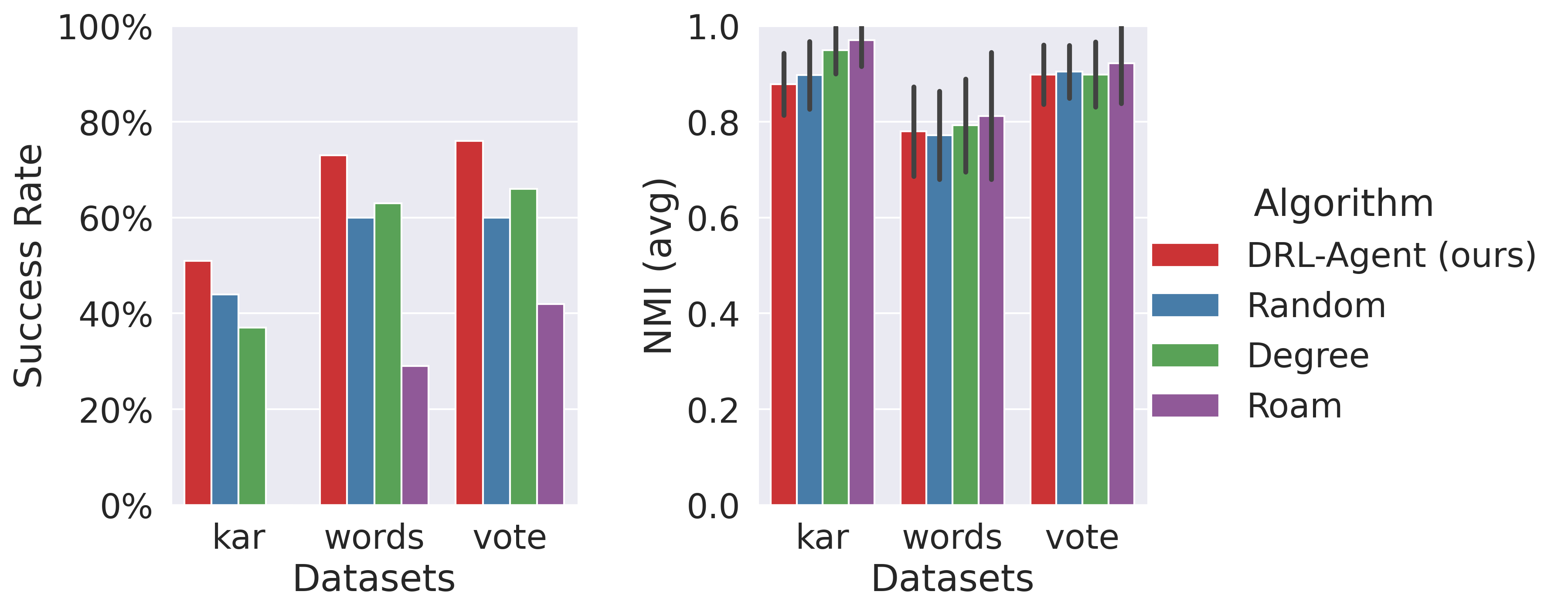
Figure 2. SR and NMI using the Greedy algorithm as $f(\cdot)$ on all datasets, with $\tau=0.3$ and $\beta=1\mu$, both at training and node deception time (symmetric).

A crucial observation is that our method strikes the best balance between the Success Rate and the NMI score. On the one hand, it achieves a higher success rate in hiding the selected target node than competing methods (reaching up to $80\%$ with an improvement of approximately $15\%$ over the best-performing baseline). On the other hand, our approach pays a limited price for this success (i.e., the modified graph remains relatively similar to the original one), as evidenced by the NMI score compared to other methods. In fact, for the words and vote datasets, the NMI score achieved by our DRL-Agent is similar to that of the baselines. In the case of the kar dataset, our method’s NMI score is slightly lower than that of, for example, Roam. However, while our method accomplishes the node deception task around $50\%$ of the time, Roam always fails.

The second key finding concerns the ability of our DRL-Agent to transfer to a different community detection algorithm (asymmetric setup). Specifically, we evaluate the performance of our method, which was trained on the modularity-based Greedy algorithm, in the context of a node deception task that utilizes a different community detection algorithm, namely the Louvain algorithm. As illustrated in Fig. 3, both the baselines and our DRL-Agent achieve even higher success rates in this asymmetric setting, with our method maintaining its superiority. Naturally, this outcome has a more substantial impact on the NMI score. However, intriguingly, the disparity between our method’s NMI and other approaches becomes even less pronounced than in the previous symmetric setup.

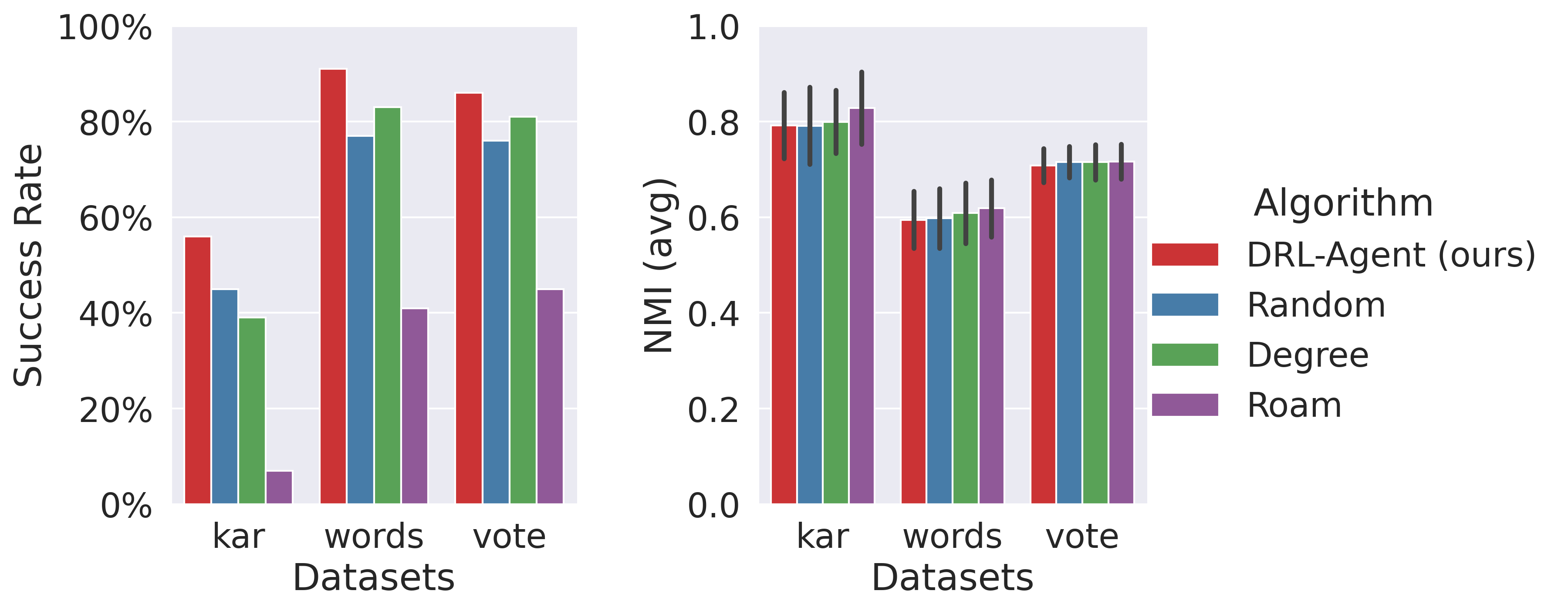
Figure 3. SR and NMI using the Greedy algorithm at training time and the Louvain algorithm at node deception time as $f(\cdot)$ on all datasets, with $\tau=0.3$, and $\beta=1\mu$ (asymmetric).

Similar conclusions can be drawn for the other community detection algorithms considered and using different combinations of values for the key parameters $\tau$ and $\beta$. The complete results for the node deception task are outlined in Appendix C.1.

Community Deception Task. We evaluate our method against the baselines outlined in Section 6.3, using the same datasets, detection algorithms, and $\tau$ constraint values as the node deception task, with the only difference being the variation of $\beta$ (${1,3,5}$) due to its distinct interpretation. For smaller to medium-sized datasets, the number of rewirings is fixed based on (Fionda and Pirrò, 2018). Conversely, for larger datasets, we define $\beta$ as a ratio of the community size to hide (e.g., $\beta=0.1|\mathcal{C}_{i}|$).

As with the node deception task, we examine two distinct scenarios: symmetric and asymmetric. The former involves our DRL-Agent trained on the same modularity-based community detection algorithm as used during deception, i.e., the Greedy algorithm. The latter, instead, assesses the agent’s capability to adapt to a different community detection algorithm (Louvain) during deception, despite being still trained on the Greedy algorithm (transferability).

In Fig. 4 and Fig. 5, we report the Deception Score ($\mathcal{H}$) and NMI score for our DRL-Agent in the symmetric and asymmetric setup, respectively.

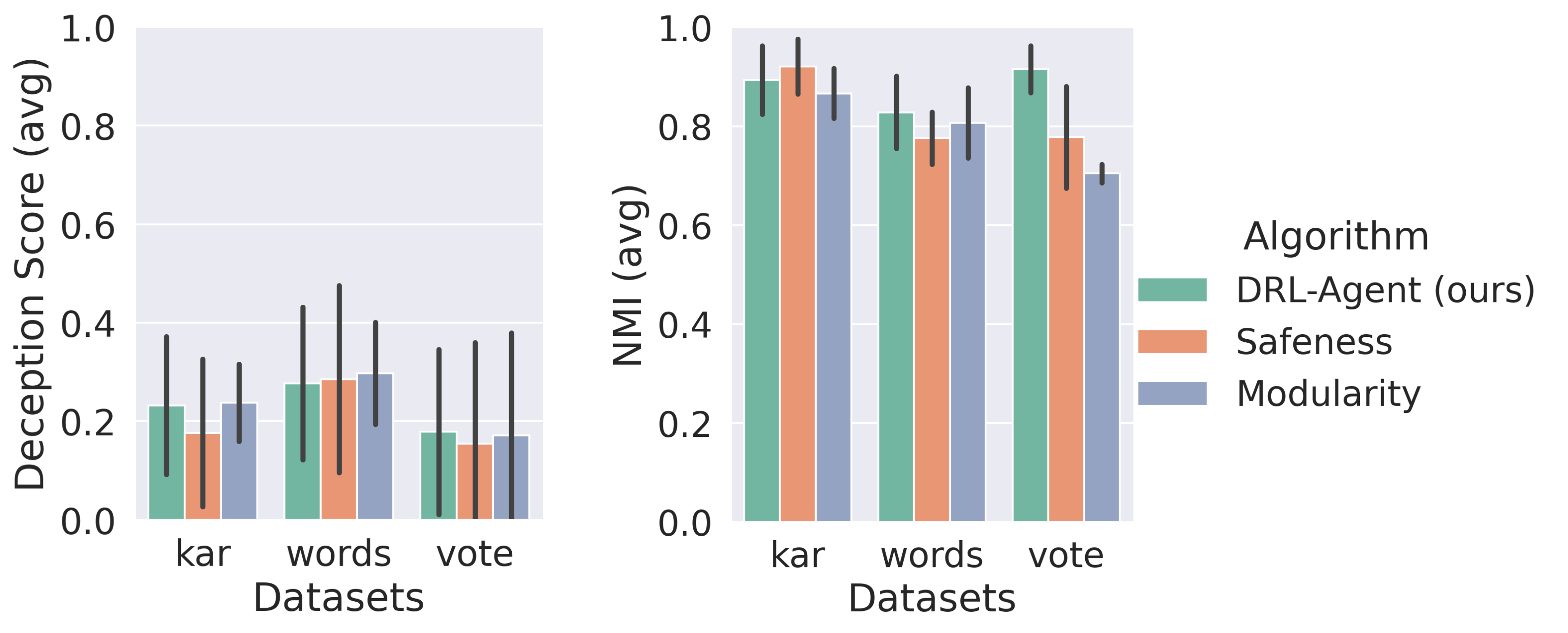
Figure 4. Deception Score ($\mathcal{H}$) and NMI using the Greedy algorithm as $f(\cdot)$ on all datasets, with $\tau=0.3$ and $\beta=1$, both at training and community deception time (symmetric).

Much like our findings in the node deception task, our approach finds the optimal trade-off between these two quality metrics. This observation holds even more significance for the larger dataset (vote), where our agent not only achieves the highest Deception Score but also the best NMI score. Moreover, our DRL-Agent demonstrates the ability to transfer its performance to a community detection algorithm that differs from the one it was trained on.

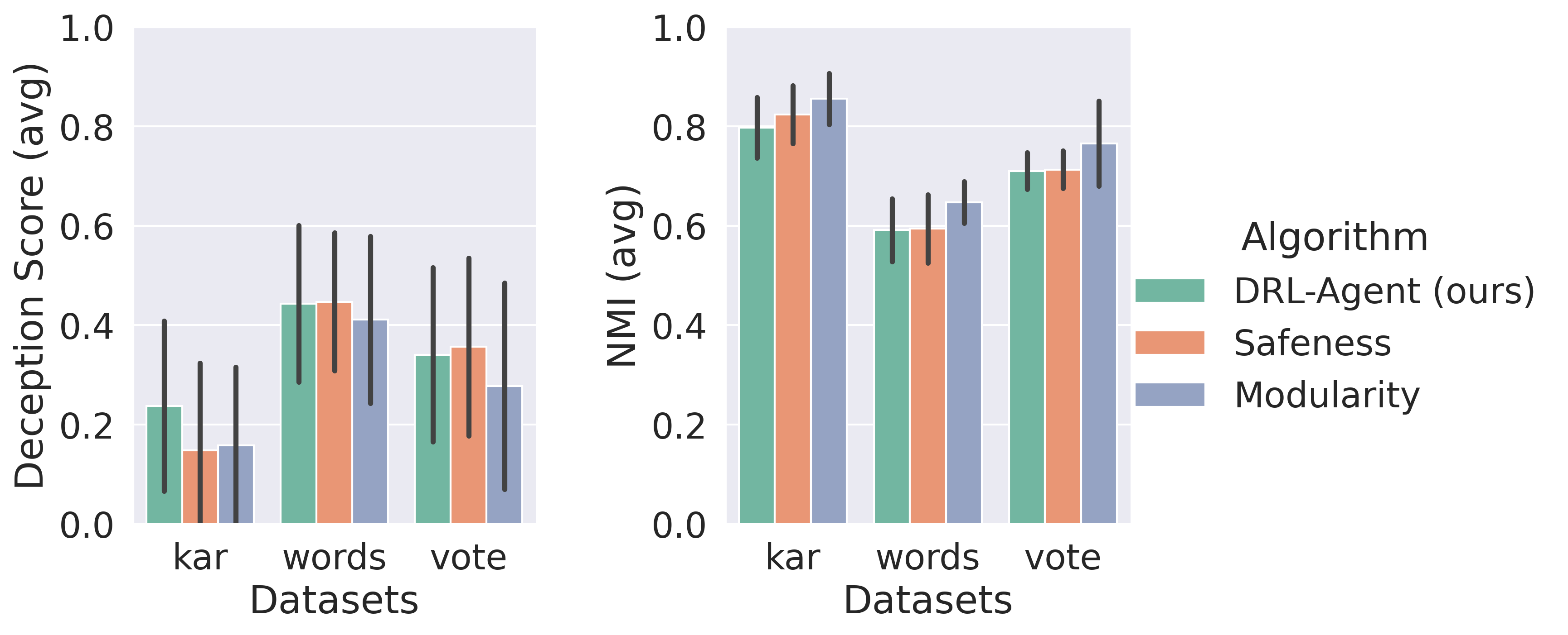
Figure 5. Deception Score ($\mathcal{H}$) and NMI using the Greedy algorithm at training time and the Louvain algorithm at community deception time as $f(\cdot)$ on all datasets, with $\tau=0.3$ and $\beta=1\mu$ (asymmetric).

In summary, across various algorithms and datasets, a common trend emerges: as the $\tau$ similarity constraint increases, the performance of the DRL-Agent on the community deception task typically decreases. This phenomenon may arise because the agent achieves the node deception objective with fewer rewirings, resulting in fewer actions targeting nodes with high centrality, as they are typically among the first analyzed by the algorithm. The full results of the community deception task can be found in Appendix C.2.

6.5. Parameter Sensitivity

The effectiveness of our DRL-Agent relies on two critical parameters: $(i)$ the similarity threshold ($\tau$) used to determine whether the node deception goal has been achieved or not, and $(ii)$ the budget ($\beta$) to limit the effort – i.e., graph modifications – performed to achieve the goal. In this section, we analyze their impact. Specifically, in Table 2 and Table 3, we explore how the SR and NMI metrics for the node deception task are influenced by varying the values of $\tau$ and $\beta$, while keeping the detection algorithm $f(\cdot)$ and dataset fixed.

Table 2. SR for node detection task, using the Greedy community detection algorithm on the words dataset.

$\bm{\tau}$	$\bm{\beta}$	Node Deception Algorithm
		DRL-Agent (ours)	Random	Degree	Roam
$0.3$	$\frac{1}{2}\mu$	$\mathbf{53}$%	$48$%	$51$%	$11$%
	$1\mu$	$\mathbf{73}$%	$60$%	$63$%	$29$%
	$2\mu$	$\mathbf{92}$%	$83$%	$84$%	$34$%
$0.5$	$\frac{1}{2}\mu$	$\mathbf{61}$%	$59$%	$\mathbf{61}$%	$13$%
	$1$$\mu$	$\mathbf{76}$%	$65$%	$73$%	$45$%
	$2\mu$	$\mathbf{96}$%	$90$%	$84$%	$47$%
$0.8$	$\frac{1}{2}\mu$	$\mathbf{78}$%	$77$%	$\mathbf{78}$%	$18$%
	$1\mu$	$\mathbf{94}$%	$93$%	$\mathbf{94}$%	$66$%
	$2\mu$	$\mathbf{100}$%	$\mathbf{100}$%	$98$%	$79$%

Table 3. NMI (avg. $\pm$ std.) for node detection task, using the Greedy community detection algorithm on the words dataset.

$\bm{\tau}$	$\bm{\beta}$	Node Deception Algorithm
		DRL-Agent (ours)	Random	Degree	Roam
$0.3$	$\frac{1}{2}\mu$	$0.79$ $\pm$ $0.08$	$0.80$ $\pm$ $0.07$	$0.80$ $\pm$ $0.10$	$\mathbf{0.95}$ $\pm$ $0.07$
	$1\mu$	$0.77$ $\pm$ $0.09$	$0.77$ $\pm$ $0.09$	$0.79$ $\pm$ $0.09$	$\mathbf{0.81}$ $\pm$ $0.13$
	$2\mu$	$0.79$ $\pm$ $0.08$	$0.78$ $\pm$ $0.08$	$\mathbf{0.80}$ $\pm$ $0.08$	$0.76$ $\pm$ $0.14$
$0.5$	$\frac{1}{2}\mu$	$0.81$ $\pm$ $0.07$	$0.79$ $\pm$ $0.08$	$0.81$ $\pm$ $0.09$	$\mathbf{0.93}$ $\pm$ $0.09$
	$1\mu$	$\mathbf{0.78}$ $\pm$ $0.07$	$0.77$ $\pm$ $0.08$	$\mathbf{0.78}$ $\pm$ $0.08$	$0.77$ $\pm$ $0.12$
	$2\mu$	$0.75$ $\pm$ $0.09$	$0.75$ $\pm$ $0.08$	$\mathbf{0.78}$ $\pm$ $0.08$	$0.75$ $\pm$ $0.12$
$0.8$	$\frac{1}{2}\mu$	$0.80$ $\pm$ $0.08$	$0.79$ $\pm$ $0.08$	$0.79$ $\pm$ $0.10$	$\mathbf{0.94}$ $\pm$ $0.10$
	$1\mu$	$0.79$ $\pm$ $0.07$	$\mathbf{0.80}$ $\pm$ $0.07$	$\mathbf{0.80}$ $\pm$ $0.08$	$0.78$ $\pm$ $0.13$
	$2\mu$	$\mathbf{0.79}$ $\pm$ $0.07$	$0.78$ $\pm$ $0.08$	$\mathbf{0.79}$ $\pm$ $0.08$	$0.74$ $\pm$ $0.11$

These results reinforce the previously mentioned findings: our method consistently achieves a superior balance between SR and NMI. Indeed, for instance, Roam has a milder impact on the graph structure, but it frequently fails to achieve the node deception goal. On the other hand, our DRL-Agent has the best success rate without overly altering the original graph.

7. Ethical Implications

As highlighted in the motivation for this work, community membership hiding algorithms can serve as valuable tools for safeguarding the privacy of social network users. Furthermore, these methods can be used to protect individuals at risk, including journalists or opposition activists, in regions governed by authoritarian regimes. Additionally, these techniques can combat online criminal activities by modifying network connections to infiltrate espionage agents or disrupt communications among malicious users.

However, node-hiding techniques can also be exploited to pursue harmful goals. For instance, malicious individuals can strategically employ these methods to evade network analysis tools, often used by law enforcement agencies for public safety, enabling them to mask their illicit or criminal activities on the network.

8. Conclusion and Future Work

This paper tackled the challenge of community membership hiding, which entails strategically modifying the structural characteristics of a network graph to prevent specific nodes from being detected by a community detection algorithm. To address this problem, we formulated it as a constrained counterfactual graph objective and employed deep reinforcement learning for its solution. We conducted extensive experiments to validate our method’s effectiveness in two distinct tasks: node and community deception. Results demonstrated that our approach strikes the best balance between achieving the deception goal and the required cost of graph modifications compared to existing baselines in both tasks.

In future work, we intend to apply our method to larger-scale graphs and integrate node feature modifications alongside graph structural alterations.

References

- (1)
- Blondel et al. (2008) Vincent D. Blondel, Jean-Loup Guillaume, Renaud Lambiotte, and Etienne Lefebvre. 2008. Fast Unfolding of Communities in Large Networks. Journal of Statistical Mechanics: Theory and Experiment 2008, 10 (oct 2008), P10008. https://doi.org/10.1088/1742-5468/2008/10/P10008
- Brandes et al. (2008) Ulrik Brandes, Daniel Delling, Marco Gaertler, Robert Görke, Martin Hoefer, Zoran Nikoloski, and Dorothea Wagner. 2008. On Modularity Clustering. IEEE Transactions on Knowledge and Data Engineering 20 (2008), 172–188. https://api.semanticscholar.org/CorpusID:150684
- Campan et al. (2015) Alina Campan, Yasmeen Alufaisan, and Traian Marius Truta. 2015. Preserving Communities in Anonymized Social Networks. Trans. Data Privacy 8, 1 (dec 2015), 55–87.
- Chen et al. (2021) Xianyu Chen, Zhongyuan Jiang, Hui Li, Jianfeng Ma, and Philip S. Yu. 2021. Community Hiding by Link Perturbation in Social Networks. IEEE Transactions on Computational Social Systems 8, 3 (2021), 704–715. https://doi.org/10.1109/TCSS.2021.3054115
- Chen et al. (2022) Ziheng Chen, Fabrizio Silvestri, Jia Wang, He Zhu, Hongshik Ahn, and Gabriele Tolomei. 2022. ReLAX: Reinforcement Learning Agent Explainer for Arbitrary Predictive Models. In Proceedings of the 31st ACM International Conference on Information & Knowledge Management, Atlanta, GA, USA, October 17-21, 2022, Mohammad Al Hasan and Li Xiong (Eds.). ACM, 252–261. https://doi.org/10.1145/3511808.3557429
- Dice (1945) Lee R. Dice. 1945. Measures of the Amount of Ecologic Association Between Species. Ecology 26, 3 (1945), 297–302. https://doi.org/10.2307/1932409 arXiv:https://esajournals.onlinelibrary.wiley.com/doi/pdf/10.2307/1932409
- Donnat and Holmes (2018) Claire Donnat and Susan Holmes. 2018. Tracking Network Dynamics: A Survey of Distances and Similarity Metrics. arXiv:1801.07351 [stat.AP]
- Fionda and Pirrò (2018) Valeria Fionda and Giuseppe Pirrò. 2018. Community Deception or: How to Stop Fearing Community Detection Algorithms. IEEE Transactions on Knowledge and Data Engineering 30, 4 (2018), 660–673. https://doi.org/10.1109/TKDE.2017.2776133
- Fortunato (2010) Santo Fortunato. 2010. Community Detection in Graphs. Physics Reports 486, 3 (2010), 75–174. https://doi.org/10.1016/j.physrep.2009.11.002
- Gammelli et al. (2021) Daniele Gammelli, Kaidi Yang, James Harrison, Filipe Rodrigues, Francisco C. Pereira, and Marco Pavone. 2021. Graph Neural Network Reinforcement Learning for Autonomous Mobility-on-Demand Systems. arXiv:2104.11434 [eess.SY]
- Girvan and Newman (2002) M. Girvan and M. E. J. Newman. 2002. Community Structure in Social and Biological Networks. Proceedings of the National Academy of Sciences 99, 12 (2002), 7821–7826. https://doi.org/10.1073/pnas.122653799 arXiv:https://www.pnas.org/doi/pdf/10.1073/pnas.122653799
- Grover and Leskovec (2016) Aditya Grover and Jure Leskovec. 2016. node2vec: Scalable Feature Learning for Networks. arXiv:1607.00653 [cs.SI]
- Jaccard (1912) Paul Jaccard. 1912. The Distribution of the Flora in the Alpine Zone. New Phytologist 11, 2 (1912), 37–50. https://doi.org/10.1111/j.1469-8137.1912.tb05611.x
- Jin et al. (2021) Di Jin, Zhizhi Yu, Pengfei Jiao, Shirui Pan, Dongxiao He, Jia Wu, Philip S. Yu, and Weixiong Zhang. 2021. A Survey of Community Detection Approaches: From Statistical Modeling to Deep Learning. arXiv:2101.01669 [cs.SI]
- Kalaichelvi and Easwarakumar (2022) N. Kalaichelvi and K. S. Easwarakumar. 2022. A Comprehensive Survey on Community Deception Approaches in Social Networks. In Computer, Communication, and Signal Processing, Erich J. Neuhold, Xavier Fernando, Joan Lu, Selwyn Piramuthu, and Aravindan Chandrabose (Eds.). Springer International Publishing, Cham, 163–173.
- Karataş and Şahin (2018) Arzum Karataş and Serap Şahin. 2018. Application Areas of Community Detection: A Review. In Proceedings of the International Congress on Big Data, Deep Learning and Fighting Cyber Terrorism (IBIGDELFT). 65–70. https://doi.org/10.1109/IBIGDELFT.2018.8625349
- Kipf and Welling (2017) Thomas N. Kipf and Max Welling. 2017. Semi-Supervised Classification with Graph Convolutional Networks. arXiv:1609.02907 [cs.LG]
- Kreer (1957) J. Kreer. 1957. A Question of Terminology. IRE Transactions on Information Theory 3, 3 (1957), 208–208. https://doi.org/10.1109/TIT.1957.1057418
- Kumari et al. (2021) Suchi Kumari, Riteshkumar Jayprakash Yadav, Suyel Namasudra, and Ching-Hsien Hsu. 2021. Intelligent deception techniques against adversarial attack on the industrial system. International Journal of Intelligent Systems 36, 5 (2021), 2412–2437.
- Lancichinetti et al. (2009) Andrea Lancichinetti, Santo Fortunato, and János Kertész. 2009. Detecting the Overlapping and Hierarchical Community Structure in Complex Networks. New Journal of Physics 11, 3 (mar 2009), 033015. https://doi.org/10.1088/1367-2630/11/3/033015
- Liu et al. (2019) Yiwei Liu, Jiamou Liu, Zijian Zhang, Liehuang Zhu, and Angsheng Li. 2019. REM: From Structural Entropy to Community Structure Deception. Curran Associates Inc., Red Hook, NY, USA.
- Lucic et al. (2022) Ana Lucic, Maartje A. ter Hoeve, Gabriele Tolomei, Maarten de Rijke, and Fabrizio Silvestri. 2022. CF-GNNExplainer: Counterfactual Explanations for Graph Neural Networks. In International Conference on Artificial Intelligence and Statistics, AISTATS 2022, 28-30 March 2022, Virtual Event (Proceedings of Machine Learning Research, Vol. 151), Gustau Camps-Valls, Francisco J. R. Ruiz, and Isabel Valera (Eds.). PMLR, 4499–4511. https://proceedings.mlr.press/v151/lucic22a.html
- Mittal et al. (2021) Shravika Mittal, Debarka Sengupta, and Tanmoy Chakraborty. 2021. Hide and Seek: Outwitting Community Detection Algorithms. IEEE Transactions on Computational Social Systems 8, 4 (2021), 799–808. https://doi.org/10.1109/TCSS.2021.3062711
- M.K and K (2016) Vijaymeena M.K and Kavitha K. 2016. A Survey on Similarity Measures in Text Mining. https://api.semanticscholar.org/CorpusID:62118842
- Mnih et al. (2016) Volodymyr Mnih, Adrià Puigdomènech Badia, Mehdi Mirza, Alex Graves, Timothy P. Lillicrap, Tim Harley, David Silver, and Koray Kavukcuoglu. 2016. Asynchronous Methods for Deep Reinforcement Learning. arXiv:1602.01783 [cs.LG]
- Mosadegh and Behboudi (2011) Mohammad Javad Mosadegh and Mehdi Behboudi. 2011. Using Social Network Paradigm for Developing a Conceptual Framework in CRM. Australian Journal of Business and Management Research 1, 4 (2011), 63.
- Nagaraja (2010) Shishir Nagaraja. 2010. The Impact of Unlinkability on Adversarial Community Detection: Effects and Countermeasures. In Privacy Enhancing Technologies, Mikhail J. Atallah and Nicholas J. Hopper (Eds.). Springer Berlin Heidelberg, Berlin, Heidelberg, 253–272.
- Newman (2006a) Mark E. J. Newman. 2006a. Finding Community Structure in Networks Using the Eigenvectors of Matrices. Phys. Rev. E 74 (Sep 2006), 036104. Issue 3. https://doi.org/10.1103/PhysRevE.74.036104
- Newman (2006b) Mark E. J. Newman. 2006b. Modularity and Community Structure in Networks. Proceedings of the National Academy of Sciences 103, 23 (June 2006), 8577–8582. https://doi.org/10.1073/pnas.0601602103
- Pons and Latapy (2005) Pascal Pons and Matthieu Latapy. 2005. Computing Communities in Large Networks Using Random Walks. (2005), 284–293.
- Raghavan et al. (2007) Usha Nandini Raghavan, Réka Albert, and Soundar Kumara. 2007. Near Linear Time Algorithm to Detect Community Structures in Large-Scale Networks. Phys. Rev. E 76 (Sep 2007), 036106. Issue 3. https://doi.org/10.1103/PhysRevE.76.036106
- Reichardt and Bornholdt (2006) Jörg Reichardt and Stefan Bornholdt. 2006. Statistical Mechanics of Community Detection. Phys. Rev. E 74 (Jul 2006), 016110. Issue 1. https://doi.org/10.1103/PhysRevE.74.016110
- Ronhovde and Nussinov (2009) Peter Ronhovde and Zohar Nussinov. 2009. Multiresolution Community Detection for Megascale Networks by Information-Based Replica Correlations. Physical Review E 80, 1 (jul 2009). https://doi.org/10.1103/physreve.80.016109
- Ruan et al. (2012) XingMao Ruan, YueHeng Sun, Bo Wang, and Shuo Zhang. 2012. The Community Detection of Complex Networks Based on Markov Matrix Spectrum Optimization. In 2012 International Conference on Control Engineering and Communication Technology. 608–611. https://doi.org/10.1109/ICCECT.2012.192
- Shannon (1948) C. E. Shannon. 1948. A Mathematical Theory of Communication. The Bell System Technical Journal 27, 3 (1948), 379–423. https://doi.org/10.1002/j.1538-7305.1948.tb01338.x
- Tolomei and Silvestri (2021) Gabriele Tolomei and Fabrizio Silvestri. 2021. Generating Actionable Interpretations from Ensembles of Decision Trees. IEEE Transactions on Knowledge and Data Engineering 33, 4 (2021), 1540–1553. https://doi.org/10.1109/TKDE.2019.2945326
- Tolomei et al. (2017) Gabriele Tolomei, Fabrizio Silvestri, Andrew Haines, and Mounia Lalmas. 2017. Interpretable Predictions of Tree-based Ensembles via Actionable Feature Tweaking. In Proceedings of the 23rd ACM SIGKDD International Conference on Knowledge Discovery and Data Mining, Halifax, NS, Canada, August 13 - 17, 2017. ACM, 465–474. https://doi.org/10.1145/3097983.3098039
- Trappolini et al. (2023) Giovanni Trappolini, Valentino Maiorca, Silvio Severino, Emanuele Rodola, Fabrizio Silvestri, and Gabriele Tolomei. 2023. Sparse Vicious Attacks on Graph Neural Networks. IEEE Transactions on Artificial Intelligence (2023).
- Waniek et al. (2018) Marcin Waniek, Tomasz P. Michalak, Michael J. Wooldridge, and Talal Rahwan. 2018. Hiding Individuals and Communities in a Social Network. Nature Human Behaviour 2, 2 (jan 2018), 139–147. https://doi.org/10.1038/s41562-017-0290-3
- Whang et al. (2015) Joyce Jiyoung Whang, David F. Gleich, and Inderjit S. Dhillon. 2015. Overlapping Community Detection Using Neighborhood-Inflated Seed Expansion. arXiv:1503.07439 [cs.SI]
- Zhao et al. (2012) Yunpeng Zhao, Elizaveta Levina, and Ji Zhu. 2012. Consistency of Community Detection in Networks Under Degree-Corrected Stochastic Block Models. The Annals of Statistics 40, 4 (2012), 2266–2292. http://www.jstor.org/stable/41806535