GRB 080710: A narrow, structured jet showing a late, achromatic peak in the optical and infrared afterglow?

Abstract

We present a possible theoretical interpretation of the observed afterglow emission of long gamma-ray burst GRB 080710. While its prompt GRB emission properties are normal, the afterglow light curves in the optical and infrared bands are exceptional in two respects. One is that the observed light curves of different wavelengths have maximum at the same time, and that the achromatic peak time, $2.2\times 10^{3}$ s after the burst trigger, is about an order of magnitude later than typical events. The other is that the observed flux before the peak increases more slowly than theoretically expected so far. Assuming that the angular distribution of the outflow energy is top-hat or Gaussian-shaped, we calculate the observed light curves of the synchrotron emission from the relativistic jets and explore the model parameters that explain the observed data. It is found that a narrowly collimated Gaussian-shaped jet with large isotropic-equivalent energy is the most plausible model for reproducing the observed afterglow behavior. Namely, an off-axis afterglow scenario to the achromatic peak is unlikely. The inferred values of the opening angle and the isotropic equivalent energy of the jet are possibly similar to those of GRB 221009A, but the jet of GRB 080710 has a much smaller efficiency of the prompt gamma-ray emission. Our results indicate a greater diversity of the GRB jet properties than previously thought.

1 Introduction

Gamma-ray bursts (GRBs) are thought to originate in relativistically moving collimated outflows, details of which are still unknown (e.g Piran, 1999; Kumar & Zhang, 2015; Zhang, 2018). Prompt GRB emissions are followed by afterglows that tell us various information on the relativistic jets. The afterglows in the X-ray, optical/infrared, and radio bands most likely arise from synchrotron radiation of high-energy electrons accelerated at relativistic shocks propagating into circumburst medium (e.g. Sari, Piran, & Narayan, 1998; Sari, Piran, & Halpern, 1999) and/or into the relativistic jets (e.g. Sari & Piran, 1999; Kobayashi & Sari, 2000). Since Neil Gehrels Swift Observatory launched, well-sampled early afterglow light curves in various wavelengths have been collected, and it has been found that they contradict the expectations from the standard afterglow model in the pre-Swift era. The observed canonical X-ray afterglow unexpectedly consists of three distinct phases (Nousek et al., 2006; Zhang et al., 2006). In the optical/infrared bands, the pre-Swift afterglow model predicted that light curves had maxima at around $\sim 10^{3-4}$ s after the prompt emission (Sari, Piran, & Narayan, 1998), and that peak times were later for lower frequencies. Such chromatic behavior has not been firmly confirmed as of yet, but instead, some bright events have shown the optical peak at $\sim 10^{2}$ s from the beginning of the prompt emission, which has been interpreted as the afterglow onset, that is, the jet deceleration becomes significant at the peak time (e.g. Molinari et al., 2007; Liang et al., 2010). In the radio bands, it has been found that for some events, like the recent bright burst GRB 221009A (Laskar et al., 2023; Bright et al., 2023), simple single-component models do not reproduce the observed light curves. At present, it may be important to study events showing observational features apparently inconsistent with pre-Swift afterglow theories. Such theoretical works may provide us hints leading to new understandings of the nature of the GRB jet.

GRB 080710 was detected by Swift Burst Alert Telescope (BAT) (Sbarufatti et al., 2008), and its duration was $T_{90}=120~{}\rm{s}$ (Tueller et al., 2008), so that this event is classified as a long GRB. Its redshift is $z=0.845$ (Perley, Chornock, & Bloom, 2008). The isotropic equivalent gamma-ray energy and rest-frame peak energy in the $\nu F_{\nu}$-spectrum were estimated as $E_{\gamma,\rm{iso}}=6\times 10^{51}$ erg and $(1+z)E_{\rm peak}\simeq 2\times 10^{2}$ keV, respectively (Krühler et al., 2009). These values are in the range of typical long GRBs observed so far (e.g. Minaev & Pozanenko, 2020; Zhao et al., 2020). The observed isotropic-equivalent luminosity $L_{\gamma,{\rm iso}}=1-8\times 10^{50}$ erg s^-1 (Lü et al., 2012; Liang et al., 2015; Ghirlanda et al., 2018) and $(1+z)E_{\rm peak}$ are also roughly consistent with Yonetoku relation (e.g. Yonetoku et al., 2004; Li, 2023). On the other hand, GRB 080710 showed unusual optical/infrared afterglow behavior (Krühler et al., 2009). The light curves in various bands have maximum at the same time at $T=T_{\rm peak}\simeq 2.2\times 10^{3}$ s, where $T$ is the observer time after the BAT trigger. Then, the r-band isotropic peak luminosity, $L_{\nu}\sim 1.6\times 10^{31}$ erg s^-1 Hz^-1, is in the same order as other events with optical afterglow detection (e.g., Nardini, Ghisellini, & Ghirlanda, 2008; Nysewander, Fruchter, & Pe’er, 2009; Cenko et al., 2009; Kann et al., 2010; Panaitescu & Vestrand, 2011; Liang et al., 2013; Panaitescu, Vestrand, & Woźniak, 2013). Before the peak, the observed flux arises with $F_{\nu}\propto T^{1.1}$. According to the pre-Swift standard model, the optical peaks should have been chromatic when they occur at $T\sim 10^{3-4}$ s, and the flux before the peak time should increase more gradually than observed ($F_{\nu}\propto T^{1/2}$: Sari, Piran, & Narayan, 1998). Although an interpretation of afterglow onset might explain the observed achromatic behavior, the observed peak time is an order of magnitude later than usual (Panaitescu & Vestrand, 2011), and then the rising part would have been more steeper than observed ($F_{\nu}\propto T^{2-3}$: Sari & Piran, 1999). Krühler et al. (2009) proposed that the observed achromatic peak is a signature of off-axis afterglow (e.g., Granot et al., 2002; van Eerten, Zhang, & MacFadyen, 2010). However, also in this case, the flux before the peak would have increased more rapidly than observed. Moreover, the prompt emission should have been dimmer and softer than observed (Ioka & Nakamura, 2001, 2018, 2019; Ramirez-Ruiz et al., 2005; Sato et al., 2021; Salafia et al., 2015, 2016; Yamazaki, Ioka, & Nakamura, 2002, 2003, 2004; Yamazaki, Yonetoku, & Nakamura, 2003). So far, similar events with late-time, achromatic optical peaks as GRB 080710 have been detected, such as GRBs 050408 (de Ugarte Postigo et al., 2007), 071031 (Krühler et al., 2009), and 080603A (Guidorzi et al., 2011).

In this paper, using Bayesian inference with the aid of Markov chain Monte Carlo (MCMC) sampling, we discuss on the possible explanation of achromatic peak of GRB 080710 afterglow. In the previous paragraph, we did not consider the angular structure of the jet, in other words, the issues on this event were based on the uniform, top-hat (TH) jet. They might be reconciled by structured jets (e.g., Rossi, Lazzati, & Rees, 2002; Zhang & Mészáros, 2002; Zhang et al., 2004; Kumar & Granot, 2003; Beniamini et al., 2020; Oganesyan et al., 2020). When the GRB jet has angular dependence of the initial kinetic energy and/or bulk Lorentz factor (that is, they are functions of the angle from the central axis of the jet), the observed afterglow light curves are different from those for the TH case. The jet structure contains rich information on the jet formation and/or propagation into dense media around the central engine (e.g., Zhang, Woosley, & MacFadyen, 2003; Morsony, Lazzati, & Begelman, 2007; Mizuta & Ioka, 2013; Gottlieb, Nakar, & Bromberg, 2021). It had long been desired to be studied until the detection of a nearby short GRB 170817A with precise multiwavelength data. A lot of authors take this opportunity to reconsider the jet structure, and it has been common that the TH jet model is difficult to explain the observation (e.g., D’Avanzo et al., 2018; Lazzati et al., 2018; Lyman et al., 2018; Margutti et al., 2018; Troja et al., 2018; Xie, Zrake, & MacFadyen, 2018; Ghirlanda et al., 2019; Ioka & Nakamura, 2019; Lamb et al., 2019; Beniamini, Granot, & Gill, 2020; Takahashi & Ioka, 2020, 2021; Mooley, Anderson, & Lu, 2022). Such argument has also been applied to long GRBs 160625 (Cunningham et al., 2020), 221009A (O’Connor et al., 2023; Sato et al., 2023; Gill & Granot, 2023; LHAASO Collaboration et al., 2023), and so on.

This paper is organized as follows. In Section 2, we introduce models of afterglow emission from the structured jets to explain the observed data of GRB 080710, and describe our fitting method. In Section 3, we show the results for the models, and discuss their differences among them. Section 4 is devoted for discussion. Following Krühler et al. (2009), we adopt the flat $\Lambda$CDM model with cosmological parameters, $H_{0}=71$ km s^-1, $\Omega_{M}=0.27$, and $\Omega_{\Lambda}=0.73$ (Spergel et al., 2003). Then, the luminosity distance is calculated as $d_{L}=1.67\times 10^{28}~{}{\rm cm}$ for the redshift $z=0.845$.

2 Afterglow Model and Fitting Method

In this section, we present afterglow emission models and a method of parameter estimation using MCMC. We use an open-source Python package afterglowpy (Ryan et al., 2020) that numerically calculates the synchrotron emission from a shell relativistically moving into uniform ambient medium with a number density $n_{0}$. Let $(r,\theta)$ be radial and polar angle coordinates in the rest frame of the central engine, located at $r=0$. The central axis of the axisymmetric jet corresponds to $\theta=0$. In this frame, we define an initial angular distribution of the isotropic equivalent energy of the shell, $E(\theta)=4\pi(dE/d\Omega)$. In this paper, we adopt two cases for $E(\theta)$: TH and Gaussian-shaped jets. The former is expressed as

$$E(\theta)=\left\{\begin{array}[]{ll}E_{0}&(\theta\leqq\theta_{j})\\ 0&(\theta>\theta_{j})\end{array}\right.~{}~{},$$ (3)

where $E_{0}$ is constant, and $\theta_{j}$ is an opening half-angle. On the other hand, the Gaussian jet model is described by

$$E(\theta)=\left\{\begin{array}[]{ll}E_{0}\exp{\left(-\frac{\theta^{2}}{2\theta_{c}^{2}}\right)}&(\theta\leqq\theta_{j})\\ 0&(\theta>\theta_{j})\end{array}\right.~{}~{},$$ (6)

where the most of the jet energy is confined in $\theta<\theta_{c}$. Note that the collimation-corrected energy of the jet is calculated as

$$E_{\rm K,jet}=2\int_{0}^{2\pi}d\phi\int_{0}^{\theta_{j}}d\theta\,\sin{\theta}\frac{E(\theta)}{4\pi}~{}~{}.$$ (7)

This integration can be approximated as $E_{\rm K,jet}\approx E_{0}\theta_{j}^{2}/2$ and $E_{\rm K,jet}\approx E_{0}\theta_{c}^{2}[1-\exp(-\theta_{j}^{2}/2\theta_{c}^{2})]$ for the TH and Gaussian jets, respectively, when $\theta_{j}\ll 1$. The angular distribution of the initial Lorentz factor of the shell, $\Gamma(\theta)$, is given in two limiting cases. One is the case of $\Gamma(\theta)=\Gamma_{0}$, where $\Gamma_{0}$ is constant, so that initial Lorentz factor is uniform in $\theta$ (Gamma-Flat: hereafter, GF). The other case is given by $\Gamma(\theta)=1+(\Gamma_{0}-1)E(\theta)/E_{0}$, so that the initial mass-loading is uniform in $\theta$ (Gamma-Even-Mass: hereafter, GEM). Then, the evolution of the bulk Lorentz factor, $\Gamma(r,\theta)$, of the emitting material moving in the direction of $\theta$ is determined from the free expansion to adiabatic deceleration phases. Once the jet dynamics is given, the observed synchrotron emission is calculated. The index of the electron energy distribution, $p$, and microphysics parameters, $\epsilon_{e}$ (the fraction of the shock internal energy that is partitioned to electron), $\epsilon_{B}$ (the fraction of the shock internal energy that is partitioned to magnetic fields), and $\xi_{N}$ (the number fraction of electrons that are accelerated to a non-thermal distribution) are assumed to be constant. Observer’s line of sight is in the direction $\theta=\theta_{\rm obs}$.

Using the Python MCMC module emcee (Foreman-Mackey et al., 2013), we perform a Bayesian estimation to determine the best-fit parameters explaining the observed data of the optical, infrared, and X-ray afterglow of GRB 080710. For the TH jet model, we will have posterior distributions for nine quantities, $E_{0}$, $\Gamma_{0}$, $\theta_{j}$, $\beta$, $n_{0}$, $p$, $\epsilon_{e}$, $\epsilon_{e}$, and $\xi_{N}$ (Table 1), while for the GF and GEM models, another quantity $\alpha$ is added (Tables 2 and 3), where we define $\alpha=\theta_{j}/\theta_{c}$ and $\beta=\theta_{\rm obs}/\theta_{j}$. We adopt log-uniform prior distributions for $E_{0}$, $n_{0}$, $\epsilon_{e}$, $\epsilon_{B}$, and $\xi_{N}$, and uniform prior distributions for $\Gamma_{0}$, $\theta_{j}$, $\alpha$, $\beta$, and $p$. We impose the condition $\alpha\geq 1$ (i.e., $\theta_{j}\geq\theta_{c}$) to have Gaussian-like structure. A general case, $0\leq\beta\leq 1.5$, and an off-axis viewing case, $1\leq\beta\leq 1.5$, as prior ranges are studied in the next section. We set $2.01\leq p\leq 2.9$ as a prior range because afterglowpy works for $p>2$. The other parameters have sufficiently wide prior range. The likelihood for each nine- or ten-parameter set is calculated by

$${\cal L}(\vec{\theta})=\prod_{k=1}^{N}\frac{1}{\sqrt{2\pi\sigma_{k}^{2}}}\exp\left({-\frac{(Y_{k}-F_{k}(\vec{\theta}))^{2}}{2\sigma_{k}^{2}}}\right),$$ (8)

where $N$ is the number of observation data points, $Y_{k}$ and $\sigma_{k}$ are the median and the standard deviation (1$\sigma$ error) of the $k$-th observed flux ($k=1,2,\cdots,N$), respectively, and $\vec{\theta}$ represents model parameters which are necessary to theoretically calculate the flux $F_{k}$. We generate 32 independent MCMC chains with $10^{5}$ steps to get the posterior distributions. In order to get the sufficiently converged samples, we discard the first $\sim 2\times 10^{4}$ steps as burn-in for TH and GF cases, while the first $\sim 1\times 10^{3}$ steps for GEM case. Samples once per 100 steps for each MCMC chain are obtained.

3 Results

In this section, the results of our parameter fitting analysis, are shown for the three cases (TH, GF, and GEM). For each case, we investigate the behavior of the best-fit model for GRB 080710 afterglow in z-band ($\nu_{z}=3.3\times 10^{14}$ Hz), r-band ($\nu_{r}=4.8\times 10^{14}$ Hz), and X-ray band ($\nu_{X}=7.3\times 10^{16}$ Hz).

The X-ray data are extracted from the Swift team website (Evans et al., 2007, 2009). The data provides us with time evolution of the integrated energy flux in the 0.3–10 keV and spectral hardness. The spectral hardness is almost constant with time, and the time-averaged photon index is $1.92^{+0.12}_{-0.11}$. Hence, we assume the photon index of 1.92 all the time to calculate the energy flux density at $h\nu_{X}=0.3$ keV. In the MCMC fitting, we adopted a uniform error of 1% for all X-ray observed data points to ensure equal weighting of the data compared to the optical/infrared ones. The r-band and z-band flux densities were taken from Krühler et al. (2009). Here, we thin out observed r-band and z-band data to get roughly equal number of data points in a logarithmic time intervals, reducing the weight of dense data from large number of observation points after the peak time. We add systematic error of 0.012 mag for both bands (see online material for Krühler et al., 2009). The values of extinction, $A_{\rm r}$ and $A_{\rm z}$, are calculated as follows. The extinctions in r-band (0.63 $\mu$m) and z-band (0.92 $\mu$m) in our Galaxy toward the direction of GRB 080710 are estimated as $A_{\rm r}^{\rm MW}=0.171~{}{\rm mag}$ and $A_{\rm z}^{\rm MW}=0.094~{}{\rm mag}$, respectively (Schlafly & Finkbeiner, 2011). Wavelengths of these lights are $\lambda=0.34~{}\mu$m and 0.50 $\mu$m at the rest frame of the host galaxy. The V-band (0.55 $\mu$m) extinction is measured as $A_{\rm V}^{\rm HG}=0.03\pm 0.01$ (Schady et al., 2012). Assuming the formula of extinction law given by Cardelli, Clayton, & Mathis (1989), we convert $A_{\rm V}^{\rm HG}$ into $A_{\lambda}^{\rm HG}$ of the other bands, and get $A_{\rm r}^{\rm HG}=0.0485~{}{\rm mag}$ and $A_{\rm z}^{\rm HG}=0.0337~{}{\rm mag}$, respectively. Hence, the total extinctions are derived as $A_{\rm r}=A_{\rm r}^{\rm HG}+A_{\rm r}^{\rm MW}=0.2195~{}{\rm mag}$ and $A_{\rm z}=A_{\rm z}^{\rm HG}+A_{\rm z}^{\rm MW}=0.1277~{}{\rm mag}$.

Median values for the one-dimensional projection of the (marginalized) posterior distributions of each model parameter, as well as the best-fit parameters, for TH, GF, and GEM models are shown in Tables 1, 2 and 3, respectively, where we set prior range $0\leq\beta\leq 1.5$. It is found that for all three cases, the median and the best-fit values are close with each other.

Table 4 summarises the best-fit parameters derived for the cases of the different prior ranges of $\beta=\theta_{\rm obs}/\theta_{j}$ such that $0\leq\beta\leq 1.5$ and $1\leq\beta\leq 1.5$. The limitation to the off-axis viewing cases (that is, the narrower prior range of $\beta$) does not produce significantly better fit for the three models (TH, GF, and GEM). Furthermore, in the case of the prior range $1\leq\beta\leq 1.5$, the best fitted values of $\beta$ is very close to unity, so that we cannot see the characteristics of the off-axis afterglow. Hence, in the following sections 3.1, 3.2, and 3.3, we explain the physical behavior of the best-fit model obtained for the general prior range $0\leq\beta\leq 1.5$.

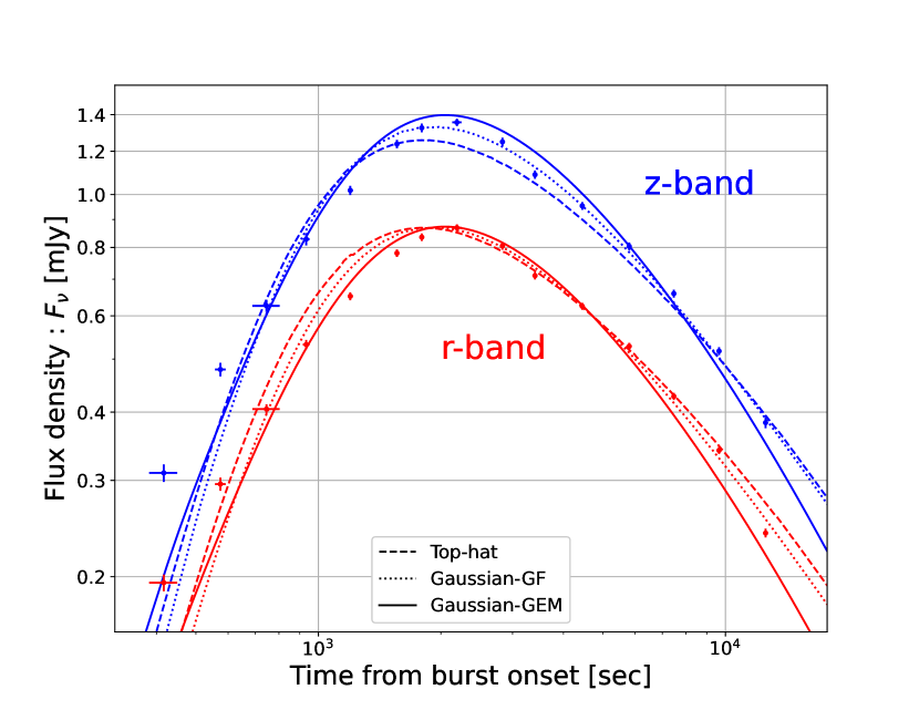
Figure 2: Enlarged view of Fig. 1 around peak time ($T\sim 2\times 10^{3}~{}{\rm s}$) in the r-band (red) and z-band (blue).

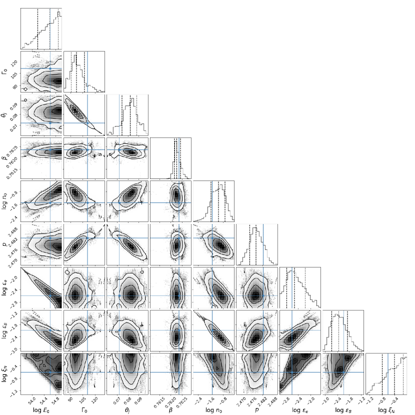
Figure 4: Posterior probability distributions of parameters by TH jet model for GRB 080710 afterglow. We assume flat prior with a range $0\leq\beta\leq 1.5$ in the MCMC sampling. Contours of 0.5, 1, 1.5, and 2$\sigma$ are shown in the two-dimensional space of all possible combinations of two model parameters. Vertical dashed lines represent the median value and 68% uncertainties (the 16% and 84% quantiles) for each parameter. Blue solid lines show the location of the best-fit parameters (giving the maximum posterior probability).

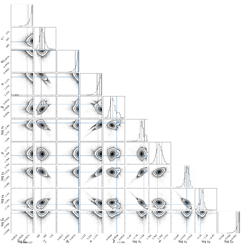
Figure 5: The same as Fig. 4 but for the GF model.

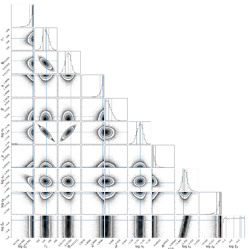
Figure 6: The same as Fig. 4 but for the GEM model.

In Fig. 1, we draw the z-band (blue), r-band (red), and X-ray (green) light curves for the best-fit parameters in the cases of TH (dashed lines), GF (dotted lines), and GEM (solid lines). Figure 2 is an enlarged view of Fig. 1, showing the differences among the three models around the peak time. In particular, the rising slope predicted by the GEM is the most gradual. We show in Fig. 3 the ratio of r-band ($F_{r}$) to z-band ($F_{z}$) fluxes. The covariances and posterior probability distributions of model parameters obtained by MCMC sampling for TH, GF, and GEM models are shown in Figs. 4, 5, and 6, respectively. As shown in Table 4, the GEM model with prior range $0\leq\beta\leq 1.5$ gives the smallest value of $\chi^{2}$/d.o.f..

In the following Sections 3.1, 3.2, and 3.3, we describe the properties of the best-fit parameter sets for TH, GF, and GEM models, respectively. For this purpose, we introduce several timescales and characteristic frequencies, which are analytically estimated in Appendix. We define $T_{\rm dec}(\theta)$ as the time at which photons emitted from the region moving into $\theta$-direction that starts to decelerate arrive at the observer, $T_{\rm beam}(\theta)$ as the time at which photons emitted from the region moving into $\theta$ whose bulk Lorentz factor satisfies $\Gamma(r,\theta)=|\theta_{\rm obs}-\theta|^{-1}$ arrive at the observer, and $T_{\rm jet}$ as the jet break time, that is, the time when the whole jet becomes visible to the observer. Note that $T_{\rm beam}(\theta)$ is defined in the case where the emission region satisfies an initial condition $\Gamma(\theta)>|\theta_{\rm obs}-\theta|^{-1}$, and the observed flux from the emitting matter with $\theta$ is dim until $T_{\rm beam}(\theta)$ due to the relativistic beaming effect. Furthermore, the emission region with $\theta$ provides characteristic frequencies, $\nu_{m}(T,\theta)$ and $\nu_{c}(T,\theta)$, at the observer time $T$, of synchrotron emission from electrons with the minimum Lorentz factor and the cooling Lorentz factor, respectively, and their crossing times $T_{m}(\theta,\nu)$ and $T_{c}(\theta,\nu)$ of the observing frequency, $\nu$, respectively.

3.1 The case of Top-hat (TH) jet

Dashed lines in Fig. 1 represent the best-fit TH model obtained in the case of prior range $0\leq\beta\leq 1.5$. The fit is not acceptable ($\chi^{2}/{\it d.o.f}=22.5$ as shown in Table 4). The posterior distributions of the model parameters are shown in Fig. 4. In particular, the posterior distribution of $\beta$ peaks around 0.76, so that the observer’s line of sight is inside the jet cone ($\theta_{\rm obs}<\theta_{j}$). Nevertheless, we perform the MCMC fitting imposing the prior range $1\leq\beta\leq 1.5$, in order to see if the observed achromatic peak is a signature of off-axis afterglow as claimed by Krühler et al. (2009). Although the fitting result becomes slightly better ($\chi^{2}/{\it d.o.f.}=18.3$ as shown in Table 4), the fit is still unacceptable, and the rising part before the peak becomes steeper, and the achromaticity around the peak disappeared (see blue thin dashed line in Fig. 3). Furthermore, the best fitted value of $\beta$ is only slightly larger than unity ($\beta-1=1.5\times 10^{-3}$), so that the off-axis afterglow rising behavior cannot be seen. Hence, below in this section 3.1, we explain the physical behavior of the best-fit model obtained for the general prior range $0\leq\beta\leq 1.5$.

Figures 1–3 show the achromatic peaks at $\sim 2\times 10^{3}$ s in the z and r-bands, though the TH model (dashed-lines) overpredicts the observed flux at $T>10^{4.5}~{}{\rm s}$. Moreover, as can be seen in Fig. 2, the rising part before the peak is steeper than observed. To understand the behavior of the light curves, let us consider the emission from the region toward us ($\theta\approx\theta_{\rm obs}$). In the TH case, if $\theta_{\rm obs}<\theta_{j}$, the shape of the light curves hardly depends on $\theta_{\rm obs}$. For our inferred parameters, the deceleration time is calculated as $T_{\rm dec}(\theta_{\rm obs})\sim 10^{3}~{}{\rm s}$ [see Eq. (A)], which is near the observed peak. We also find $\nu_{m}(T,\theta_{\rm obs})<\nu_{z}<\nu_{r}<\nu_{c}(T,\theta_{\rm obs})$ around $T=T_{\rm dec}(\theta_{\rm obs})$. Then, the r-band and z-band fluxes behave as $F_{\nu}\propto T^{3}$ for $T<T_{\rm dec}(\theta_{\rm obs})$ (Sari & Piran, 1999), and $F_{\nu}\propto T^{-3(p-1)/4}=T^{-1.11}$ for $T>T_{\rm dec}(\theta_{\rm obs})$ and $p=2.48$ (Sari, Piran, & Narayan, 1998). Therefore, the r-band and z-band light curves take maximum simultaneously at $T\sim T_{\rm dec}(\theta_{\rm obs})$ due to the transition from the free expansion to the deceleration phases.

The deceleration time $T_{\rm dec}(\theta_{\rm obs})\sim 10^{3}~{}{\rm s}$ requires $E_{0}=4\times 10^{54}$ erg that is somewhat larger than the value of typical long GRBs. Since $T_{\rm dec}(\theta_{\rm obs})\propto(E_{0}/n_{0})^{1/3}\Gamma_{0}^{-8/3}$ [see Eq. (A)], we might have small $n_{0}$ and/or $\Gamma_{0}$ keeping smaller $E_{0}$ ($\sim 10^{52-53}$ erg). However, in this case, the peak flux at $T_{\rm dec}(\theta_{\rm obs})$, which is calculated as $F_{\rm peak}\propto\xi_{N}^{-0.48}\epsilon_{e}^{1.48}\epsilon_{B}^{0.84}n_{0}^{0.84}\Gamma_{0}^{2.96}E_{0}$ for $p=2.48$, should have been smaller than observed. Once $E_{0}$ is large, small value of $\epsilon_{e}=2.5\times 10^{-3}$ is necessary for the observed peak flux of $\sim 1$ mJy.

The cooling break in the observed spectrum by emitting matter moving toward the observer, $\nu_{c}(T,\theta_{\rm obs})$, crosses the X-ray band at $T_{c}(\theta_{\rm obs},\nu_{X})\sim 7\times 10^{2}~{}{\rm s}$ [see Eq. (21)], after which $\nu_{c}(T,\theta_{\rm obs})<\nu_{X}$. Since inferred electron spectral index is $p=2.48$, the X-ray photon index should have been $(p/2)+1=2.24$ in the epoch of X-ray observation ($T\gtrsim 3\times 10^{3}$ s). This may be inconsistent with the observed value of $1.92_{-0.11}^{+0.12}$. It is also found that around $T_{c}(\theta_{\rm obs},\nu_{X})\sim 7\times 10^{2}$ s, rising slope of the X-ray light curve changes to be shallower, leading to the slightly earlier maximum compared with r and z-bands (see Fig. 1).

As shown in Fig. 1, the power-law decay after the peak time $T_{\rm peak}$ lasts until $T\sim 6\times 10^{5}$ s, which is followed by more rapid decay. This steepening can be interpreted to be the jet break, that is, the transition to the jetted afterglow phase, because we estimate the jet break time as $T_{\rm jet}\sim 10^{6}$ s [see Eq. (18)].

3.2 The case of Gaussian jet 1: Gamma-Flat (GF)

The best-fit GF model obtained by MCMC sampling with the prior range $0\leq\beta\leq 1.5$ (Table 2) provides the afterglow light curves shown in dotted lines in Fig. 1. In this case, the value of reduced chi-squared is 24.7, so that the fit is not acceptable. The posterior distributions of the model parameters are shown in Fig. 5. The MCMC fitting for the GF model infers large $E_{0}$ ($\sim 10^{55}$ erg), $\theta_{j}$ ($\sim 0.5$ rad), and $\xi_{N}$ ($\sim 1$), all of which are near the upper end of each prior range. Since we adopt sufficiently wide prior ranges on these parameters taking into account the values of other long GRBs (e.g., Zhao et al., 2020), the GF model is already inadequate for an explanation of the observed data. As seen in the TH case (see Table 4 and § 3.1), it might be possible that if we take narrower prior range for $\beta$ (that is, $1.0<\beta<1.5$), the fit would become better. It is also to be studied for structured jets if the off-axis viewing case for the achromatic peak is viable as proposed by Krühler et al. (2009). However, the MCMC result for the case of $1.0<\beta<1.5$ is almost unchanged (see Table 4). Hence, in the following of this subsection, we briefly present the physical explanation of the model with the best-fit parameter set obtained for the prior range $0\leq\beta\leq 1.5$.

Figures 1 and 2 show that the model provides optical/infrared achromatic peak at $\sim 10^{3}$ s. The r-band and z-band fluxes roughly obeys the scaling, $F_{\nu}\propto T^{3}$, before the peak. Since the initial jet energy $E(\theta)$ has angular dependence, the quantitative discussion is limited. However, the behavior of the best-fit model can be qualitatively understood as in the following. Using the inferred values listed in Table 2, we find initially $\theta_{\rm obs}>\theta_{j}$ and $\Gamma_{0}(\theta_{\rm obs}-\theta_{j})=0.66(<1)$, so that the emission from the jet edge ($\theta=\theta_{j}=0.592$ rad) can be seen from the observer before the beginning of the jet deceleration. Since $\Gamma(\theta)=\Gamma_{0}$ for the GF model (Section 2), we approximately obtain $T_{\rm dec}(\theta)\propto\exp{(-\theta^{2}/6\theta_{c}^{2})}$ for the emission region moving in the direction $\theta$ whose range is $0.590~{}{\rm rad}\approx(\theta_{\rm obs}-\Gamma_{0}^{-1})<\theta\leq\theta_{j}$ [see Eq. (A)], and we find $T_{\rm dec}(\theta_{j})\sim T_{\rm dec}(\theta_{\rm obs}-\Gamma_{0}^{-1})\sim 10^{3}$ s, which is comparable to the observed peak time $T_{\rm peak}$. The emission from the region with $\theta<\theta_{\rm obs}-\Gamma_{0}^{-1}$ is very dim and negligible until $T\sim T_{\rm beam}(\theta_{\rm obs}-\Gamma_{0}^{-1})$. Since $T_{\rm beam}(\theta_{\rm obs}-\Gamma_{0}^{-1})\sim 10^{3}$ s, the observed flux around $T_{\rm peak}$ is dominated by the emission region with $0.590~{}{\rm rad}\lesssim\theta\leq\theta_{j}$. At early time the jet is in the free expansion phase, and we numerically find $\nu_{m}(T,\theta)<\nu_{z}<\nu_{r}<\nu_{X}<\nu_{c}(T,\theta)$, resulting in the scaling for the rising part, $F_{\nu}\propto T^{3}$, for $T<T_{\rm dec}(\theta)$. In particular, the numerically calculated light curves shown in Fig. 1 can be well explained by this scaling until $T\sim 6\times 10^{2}$ s. Between $T\sim 6\times 10^{2}$ s and the peak time $T_{\rm peak}$, the total flux is partially contributed by the decelerating region, which has $T_{m}(\theta,\nu_{z})<T_{\rm dec}(\theta)$ and $\nu_{m}(T,\theta)<\nu_{z}<\nu_{r}<\nu_{c}(T,\theta)<\nu_{X}$. Hence, the optical/infrared peak is achromatic. After the peak, the flux scales as $F_{\nu}\propto T^{-3(p-1)/4}=T^{-1.3}$ with $p=2.77$, resulting in slow decay, overshooting observed r-band and z-band data taken in the late epoch ($T\sim 3\times 10^{5}$ s). The X-ray photon index is predicted as $p/2+1=2.39$, which is inconsistent with the observed value of $1.92_{-0.11}^{+0.12}$. Similarly to the TH case, the large value of $E_{0}=1\times 10^{55}$ erg and the small value of $n_{0}=2\times 10^{-2}~{}{\rm cm^{-2}}$ as well as $\epsilon_{e}=0.01$ are necessary for $T_{\rm dec}(\theta_{j})\sim T_{\rm peak}\sim 10^{3}$ s and the observed peak flux of $\sim{\rm mJy}$.

The emission from the region moving into the direction $\theta$ that is much smaller than $\sim(\theta_{\rm obs}-\Gamma_{0}^{-1})=0.590$ rad (that is, $\Gamma_{0}(\theta_{\rm obs}-\theta)>1$) is negligible to the observed flux around $T_{\rm peak}$. We find, from Eqs. (A) and (A), $T_{\rm dec}(\theta)\propto(\theta_{\rm obs}-\theta)^{2}\exp{(-\theta^{2}/6\theta_{c}^{2})}$, which increases with decreasing $\theta$, and the ratio $T_{\rm beam}(\theta)/T_{\rm dec}(\theta)=[\Gamma_{0}(\theta_{\rm obs}-\theta)]^{2/3}>1$. The flux that is received by the observer from the region with $\theta$ takes maximum at $T_{\rm beam}(\theta)$ if $T_{\rm dec}(\theta)<T_{\rm beam}(\theta)$. For example, these characteristic times for $\theta=\theta_{c}=0.50$ rad are $T_{\rm dec}(\theta_{c})\sim 10^{5}$ s and $T_{\rm beam}(\theta_{c})\sim 10^{6}$ s. Moreover, due to the relativistic beaming effect, such emission is dim.

Using Eq. (18), we calculate the jet break time as $T_{\rm jet}\sim 10^{9}$ s. This large value comes from the large value of $E_{0}$ and wideness of the jet ($\theta_{j}\approx 0.6$ rad). Hence, relatively shallow decay lasts for a long time (see Fig. 1).

3.3 The case of Gaussian jet 2: Gamma-Even-Mass (GEM)

Solid lines in Fig. 1 represent light curves for the best-fit GEM model (Table 3) obtained by MCMC sampling with a prior range $0\leq\beta\leq 1.5$. Figure 6 shows the posterior distributions of the model parameters. In this case, we obtained the smallest value of $\chi^{2}/{\it d.o.f.}(=10.5)$ in this study, although the fit is still unacceptable. We again try to perform fitting with the prior range $1\leq\beta\leq 1.5$. However, in this case, we find that the initial bulk Lorentz factor at the jet edge satisfies $\Gamma(\theta_{j})(\theta_{j}-\theta_{\rm obs})<1$ (see Table 4), so that the characters of the off-axis afterglow do not appear. Hence, in this section, we again consider the best-fit model obtained for the prior range $0\leq\beta\leq 1.5$.

As shown in Figs. 1 and 2, this model also gives us optical/infrared achromatic peak at $2\times 10^{3}$ s. Compared with TH and GF models, GEM model gives shallower rising part before the peak, while steeper decay slope after the peak. This fact explains the observed late-time r-band and z-band fluxes at $T\sim 3\times 10^{5}$ s. Hence, reduced chi-squared in this case is the smallest among the model we tried. Below, we qualitatively explain the behavior of the best-fit model. Observer’s line of sight almost coincides with the central axis of the jet ($\theta_{\rm obs}\approx 0$). One obtains $\Gamma(\theta_{j})\simeq 15~{}(<\Gamma_{0}=1.0\times 10^{2})$ from inferred the best-fit parameters shown in Table 3. The jet is narrower ($\theta_{j}=0.024$ rad) than the TH and GF models. Hence, we get $\Gamma(\theta_{j})|\theta_{\rm obs}+\theta_{j}|<1$, so that the whole jet emission comes to the observer from the beginning. In such a case, an important timescale for the jet kinematics is $T_{\rm dec}(\theta)$.

Using Eq. (A), we find $T_{\rm dec}(\theta_{\rm obs})\sim 10^{3}~{}{\rm s}$, which is on the same order as the observed peak time $T_{\rm peak}$. Furthermore, it is found from Eqs. (A) and (A) that for $T>5\times 10^{2}~{}{\rm s}$, characteristic frequencies satisfy $\nu_{m}(T,\theta_{\rm obs})<\nu_{c}(T,\theta_{\rm obs})<\nu_{z}~{}(<\nu_{r}<\nu_{X})$. Then, the observed fluxes in z-band, r-band, and X-ray band increases according to $F_{\nu}\propto T^{2}$, and takes maximum simultaneously at $T\sim T_{\rm dec}(\theta_{\rm obs})$. Compared with the TH and GF cases, the GEM model gives more slowly rising part. Again, the large value of $E_{0}=1\times 10^{55}$ erg and the small values $n_{0}=2\times 10^{-2}~{}{\rm cm^{-2}}$ and $\epsilon_{e}=1\times 10^{-2}$ are necessary for $T_{\rm dec}(\theta_{\rm obs})\sim T_{\rm peak}\sim 10^{3}$ s and the observed peak flux of $\sim 1$ mJy. A large value of $\epsilon_{B}\simeq 0.5$ is responsible for efficient radiative energy loss of electrons to satisfy $\nu_{c}(T,\theta_{\rm obs})<\nu_{z}$ for $T<T_{\rm dec}(\theta_{\rm obs})$.

After $T\sim T_{\rm dec}(\theta_{\rm obs})=2\times 10^{3}$ s, the emission from angularly separated regions, having the polar angle $\theta$, arrives at the observer, and it becomes brightest at $T=T_{\rm dec}(\theta)$. We obtain, from Eqs. (6) and (A), $T_{\rm dec}(\theta)\propto\exp{(-\theta^{2}/6\theta_{c}^{2})}[1+(\Gamma_{0}-1)\exp{(-\theta^{2}/2\theta_{c}^{2})}]^{-8/3}$, that increases with $\theta$ for $0\leq\theta\leq\theta_{j}$. For our parameters, we get $T_{\rm dec}(\theta_{\rm obs}\approx 0)\sim 10^{3}$ s, $T_{\rm dec}(\theta_{c})\sim 10^{4}$ s, and $T_{\rm dec}(\theta_{j})\sim 10^{5}~{}{\rm s}$. The maximum flux at $\sim T_{\rm dec}(\theta)$ made by the region with $\theta$ more rapidly decreases with $\theta$ than in the case of TH jet, because $E(\theta)$ decreases with $\theta$. Therefore, for $T>T_{\rm dec}(\theta_{c})$ the total observed flux decays steeply. In this epoch, the decay slope is consistent with the scaling for jetted afterglow without rapid deceleration due to the sideway expansion in the slow cooling phase ($\nu_{m}(T,\theta)<\nu_{c}(T,\theta)<\nu_{z}<\nu_{r}<\nu_{X}$) as $F_{\nu}\propto T^{-(3p+1)/4}\propto T^{-1.76}$ in z-band, r-band, and X-ray band (Panaitescu, Mészáros, & Rees, 1998). For our parameters, $\nu_{m}(T,\theta_{\rm obs})<\nu_{c}(T,\theta_{\rm obs})<\nu_{X}$ in the decay phase [see Eqs. (A) and (A)], so that the X-ray photon index is predicted as $p/2+1=2.01$ for $p=2.01$, which is consistent with the observed value of $1.92_{-0.11}^{+0.12}$.

As shown in Fig. 6, the parameters $E_{0}$, $\alpha$ and $\epsilon_{B}$ reach the margin. It is unlikely to expand the upper bound of the prior range of $\epsilon_{B}$ beyond 0.5 $(\log(\epsilon_{B})=10^{-0.3})$. We attempted the MCMC fitting with extended prior ranges, $50<\log(E_{0})<57$ and $1<\alpha<3$. In this case, the best-fit parameters are: $E_{0}=1.17\times 10^{56}~{}{\rm erg}$, $\Gamma_{0}=160.70$, $\theta_{c}=7.64\times 10^{-3}~{}{\rm rad}$, $\alpha=2.50$, $\beta=5.95\times 10^{-3}$, $n_{0}=1.29\times 10^{-2}~{}{\rm cm^{-3}}$, $p=2.01$, $\epsilon_{e}=1.01\times 10^{-3}$, $\epsilon_{B}=4.82\times 10^{-1}$, and $\xi_{N}=0.676$. The reduced chi-squared is $923/(96-10)=10.7$, so the fit is not significantly improved. The 1D posterior distributions of $E_{0}$ and $\alpha$ take maximum at larger values, $E_{0}\sim 1\times 10^{56}$ erg and $\alpha\sim 2.5$, respectively. Then, the collimation corrected energy is calculated as $E_{\rm K,jet}\sim 7\times 10^{51}$ erg, which is too large for the peak energy of the prompt emission $(1+z)E_{\rm peak}\simeq 2\times 10^{2}$ keV (Zhao et al., 2020). Our choice of the prior range, $50<\log(E_{0})<55$, provides the result that is consistent with previous observations for $E_{\rm K,jet}$.

3.4 Model Comparison

In any models (TH, GF, and GEM), we need large values of $E_{0}$ ($\sim 10^{54-55}$ erg) to explain the late-time ($\sim 2\times 10^{3}$ s) achromatic peak in the optical/infrared bands. Even if we impose off-axis viewing $\beta=\theta_{\rm obs}/\theta_{j}\geq 1$ in the fitting, the results are not drastically improved for the three cases (see Table 4). The jets with large kinetic energy start to decelerate later than usual, making the achromatic peak. This seems to best explain the observed result of GRB 080710. The collimation-corrected energy, $E_{\rm K,jet}$, of the jet in the cases of prior range $0\leq\beta\leq 1.5$ are calculated as $1.2\times 10^{52}$, $1.2\times 10^{54}$, and $1.3\times 10^{51}~{}{\rm erg}$ for the best-fit parameters of TH, GF, and GEM models, respectively. The GF model provides much larger value than the other events (Zhao et al., 2020), which is energetically disfavored.

All six cases presented in this paper gave $\chi^{2}$/d.o.f. $>10$ (see Table 4), so that the fit is not acceptable. However, we see the differences between the $\chi^{2}$ for TH and GEM models (with prior range $\beta\geq 0$) as $\Delta\chi^{2}=\chi^{2}_{\rm TH}-\chi^{2}_{\rm GEM}=1042$, and for GF and GEM models (with prior range $\beta\geq 0$) as $\Delta\chi^{2}=\chi^{2}_{\rm GF}-\chi^{2}_{\rm GEM}=1224$, while $\Delta$(d.o.f) $=$ (d.o.f)${}_{\rm TH}-$ (d.o.f)${}_{\rm GEM}=1$ and $\Delta$(d.o.f) $=$ (d.o.f)${}_{\rm GF}-$ (d.o.f)${}_{\rm GEM}=0$. Using the $\chi^{2}$-distribution with freedom of unity, we obtain both p-value less than $10^{-15}$. Hence, the GEM model is the best representing the data among the three models TH, GF, and GEM.

Figure 3 shows the r-band to z-band flux ratio, $F_{r}/F_{z}$, for six models listed in Table 4. One can see that the observed data (black points) is achromatic around the peak time $T_{\rm peak}$. Thick and thin lines are for cases of different prior ranges $0\leq\beta\leq 1.5$ and $1\leq\beta\leq 1.5$, respectively. Both GEM (red solid lines) and GF (green dashed lines) models are roughly consistent with observation, explaining the achromatic peak. The TH (blue dotted lines) models do not fit the data well. In particular, the TH model with the prior range $1\leq\beta\leq 1.5$ shows the change of the flux ratio around $T_{\rm peak}$. In this case ($\theta_{\rm obs}>\theta_{j}$), since initially $\Gamma_{0}(\theta_{\rm obs}-\theta_{j})<1$, the off-axis afterglow character does not appear. Then, we find the break frequency $\nu_{c}(T,\theta_{j})$ crosses r and z bands in the free expansion phase and their crossing times satisfy $T_{c}(\theta_{j},\nu_{r})\lesssim T_{c}(\theta_{j},\nu_{z})\sim 2\times 10^{3}$ s. Hence, the peak times of r and z-band light curves are different, resulting in the chromatic behavior around $T_{\rm peak}$ for the TH model.

4 Discussion

Using Bayesian inference with MCMC, we have found a possible scenario of observed afterglows of GRB 080710 showing achromatic optical/infrared peak at $T_{\rm peak}=2.2\times 10^{3}$ s after the burst trigger. One of Gaussian jet models, GEM, best describes the data. Since the jet has large initial isotropic-equivalent energy ($E_{0}\sim 10^{55}$ erg), the jet deceleration starts at $T\sim 2\times 10^{3}$ s, which is responsible for the observed achromatic peak. Although $E_{0}$ is very large, the jet is narrow ($\theta_{j}=2.4\times 10^{-2}$ rad), so that the value of collimation-corrected jet energy is normal, $E_{\rm K,jet}=1.3\times 10^{51}$ erg. Note that off-axis afterglow interpretation may be unlikely, which is consistent with the observed bright and hard prompt emission.

Since two observation frequencies $\nu_{z}$ and $\nu_{r}$ are close to each other, one may expect that the peak is caused by the crossing of $\nu_{m}(T,\theta)$ to the observed band. However, we disfavor this possibility. For example, the frequency $\nu_{m}(T,\theta)$ decreases in the adiabatically expanding TH jets through the uniform ambient medium. Then, for $\Gamma(r,\theta)|\theta_{\rm obs}-\theta_{j}|<1$, we obtain the ratio of the crossing time as $T_{m}(\theta,\nu_{z})/T_{m}(\theta,\nu_{r})=(\nu_{z}/\nu_{r})^{-2/3}\sim 1.3$ [see Eq. (22)], which should be significantly larger than observed. Krühler et al. (2009) analyzed the unthinned observation data and concluded that the peak is achromatic with high measurement accuracy (see their section 3.2.), that is, $T_{m}(\theta,\nu_{z})/T_{m}(\theta,\nu_{r})\approx 1$. Furthermore, if the peak is made due to the $\nu_{m}$ crossing, then the flux ratio $F_{r}/F_{z}$ becomes larger than unity — typically, $F_{\nu}\propto\nu^{1/3}$ for $\nu<\nu_{m}$, so that one can find $F_{r}/F_{z}=(\nu_{r}/\nu_{z})^{1/3}>1$ before the peak time. However, as shown in Fig. 3, the observed flux ratio $F_{r}/F_{z}$ is always less than unity with a fixed value before and after the peak time.

Our best-fit GEM model has r-band and z-band light curves with more slowly rising part before the peak time compared with the other models, TH and GF (see Fig. 2 and § 3.3). Moreover, our GEM model shows more rapid decay after the peak time. In general, jets in the GEM model have an edge at which initial bulk Lorentz factor $\Gamma(\theta_{j})$ is smaller than that in the central part, $\Gamma(0)$. Hence, the beaming cone of the emission at the jet edge is wider, so that the jet edge effects more easily appear for the GEM model. In particular, for our the best-fit parameters, since the jet is narrowly collimated ($\theta_{j}=0.02$ rad), the jet edge can be seen from the observer from the beginning, resulting in the variation of light-curve shape around and after the peak time. In this way, the jet structure in the polar angle direction affects the observed afterglow behavior. Although the achromaticity around the peak is reproduced, the values of reduced chi-squared indicates that the fit is not acceptable. As shown in Fig. 2, the GEM model underpredicts the observed first ($T\approx 4.2\times 10^{2}$ s) and the second ($T\approx 5.7\times 10^{2}$ s) data points, although the difference is within a factor of two. More complicated jet structure might be necessary to better explain the rising part. Indeed, the hydrodynamics simulations have shown the angular dependence of the bulk Lorentz factor that is more complicated than the Gaussian shape (e.g., Zhang, Woosley, & MacFadyen, 2003; Morsony, Lazzati, & Begelman, 2007; Mizuta & Ioka, 2013; Gottlieb, Nakar, & Bromberg, 2021). Another possibility for the better fit to the observation is to consider the non-uniform circumburst medium like wind profile. These issues are beyond the scope of this paper, and will be discussed in the future work.

We estimate the efficiency of the prompt emission, $\eta_{\gamma}=E_{\rm\gamma,iso}/[E_{\rm\gamma,iso}+E(\theta_{\rm obs})]$, where $E(\theta_{\rm obs})$ is the initial kinetic energy of the afterglow jet along the observer’s line of sight. For the three cases, TH, GF, and GEM, we found $E(\theta_{\rm obs})\sim 10^{54-55}~{}{\rm erg}$, so that we obtain $\eta_{\gamma}\sim 10^{-4}$–$10^{-3}$. This value is much smaller than inferred values so far (e.g., Lloyd-Ronning & Zhang, 2004; Beniamini, Nava, & Piran, 2016). The jet of GRB 080710 has large energy but the radiation efficiency of the prompt emission is small. A possible reason for the low prompt efficiency is less turbulent flow in the GRB jet — for example, small velocity difference in the radial direction — resulting in the inefficient internal dissipation.

Since the deceleration time scales as $T_{\rm dec}\propto\Gamma_{0}^{-8/3}$, one may expect that the late-time achromatic peak arises for baryon-loaded jets (dirty fireballs) with initial bulk Lorentz factor of around 30. Taking into account this possibility, we have taken the flat prior with a range $10\leq\Gamma_{0}\leq 500$, and searched for the best-fit parameters. Then, we have obtained the posterior distribution indicating $\Gamma_{0}\gtrsim 100$. For the best-fit parameters, one can find $\Gamma(\theta_{\rm obs})\gtrsim 100$. In practice, if we take $\Gamma_{0}=30$–50, $E_{0}\sim 10^{52}~{}{\rm erg}$, and $\theta_{\rm obs}=0$ in order for the jet to have $T_{\rm dec}\sim 10^{3}~{}{\rm s}$, then the peak flux becomes much smaller than observed. The brightness at the peak time ($\sim 1$ mJy at infrared/optical) is also a strict constraint on the modeling.

As introduced in Section 1, GRB 080710 had the prompt emission properties, $E_{\gamma,\rm{iso}}=6\times 10^{51}$ erg, $(1+z)E_{\rm peak}\simeq 2\times 10^{2}$ keV and $L_{\gamma,{\rm iso}}=1-8\times 10^{50}$ erg s^-1, and we have found, in this paper, the initial bulk Lorentz factor of the afterglow jet, $\Gamma_{0}\approx 1-2\times 10^{2}$. It is believed to be the same as bulk Lorentz factor of the emitting region of the prompt emission. These are within typical range of values (e.g., Liang et al., 2010, 2015; Lü et al., 2012; Ghirlanda et al., 2018).

Our result indicates that GRB 080710 occurred in the rarefied medium ($n_{0}\sim 10^{-2}$ cm^-3). Recent bright event GRB 221009A might also arise in the small-density region (e.g., Sato et al., 2023). Such events may appear in bubbles made by strong wind from progenitor stars or in superbubbles made by OB association. Furthermore, existence of the low-density region has also been identified by three-dimensional magnetohydrodynamics simulations for a part of interstellar medium of star forming galaxies (de Avillez & Breitschwerdt, 2005).

We also attempted the MCMC fitting with the power-law jet model, $E(\theta)=E_{0}(1+\theta^{2}/b\theta_{c}^{2})^{-b/2}$ for $\theta<\theta_{j}$, using the same conditions as those of the Gaussian-GEM model. Then, we obtained the best-fit model with reduced chi-squared of $782/(96-11)=9.2$. The fit is not significantly improved, although this value is slightly lower than that for the Gaussian-GEM model of $10.5$. This result is reasonable because the functional forms of both power-law and Gaussian models are identical, $E(\theta)\sim E_{0}(1-\theta^{2}/2\theta_{c}^{2})$, for small $\theta$. Hence, our basic claim for GRB 080710 afterglow — that is, a narrow, structured jet with $E_{0}\sim 10^{55}$ erg — remains unchanged even if the power-law jets are considered.

Our results indicate that there is a diversity of GRB jets, in particular, the existence of narrowly collimated outflows with large isotropic equivalent kinetic energy but very low efficiency of the prompt emission. However, such GRB events may be difficult to be triggered since their solid angle is smaller than that of typical events so far. The prompt emission from misaligned jets is dim but their external shock emission might be detectable as orphan afterglows. Event rate of such phenomena is difficult to be calculated since we do not precisely know the fraction of the narrow jets with the large isotropic kinetic energy. The population of narrow structured jets may be studied through the other events (GRBs 050408, 071031, 080603A) that possess similar afterglow properties to GRB 080710, which will be done in future work. The multi-color follow-up observations are important to study if observed afterglow peak is achromatic or not.

In this paper, we propose the large isotropic equivalent kinetic energy of the jet ($E_{0}\sim 10^{55}$ erg) for GRB 080710 afterglow, while the small opening angle of the jet $\theta_{j}$ makes the collimation-corrected jet energy $E_{\rm K,jet}$ normal for TH and GEM cases. This situation may be similar to the case of GRB 221009A (Laskar et al., 2023; Sato et al., 2023; LHAASO Collaboration et al., 2023). However, in the case of GRB 080710, the energy of the prompt gamma-ray emission is much smaller (i.e., $\eta_{\gamma}\ll 1)$, while for GRB 221009A the isotropic equivalent gamma-ray and afterglow kinetic energies are comparable. Such kind of “monster” events like GRB 080710 with low gamma-ray emission efficiency might release their energy in the different form, that is, they might be the source of ultra-high-energy cosmic rays and/or neutrinos.

Appendix A Analytical estimate of characteristic times and frequencies, and the peak flux

In this Appendix, we present analytical formulae for characteristic timescales for an observer, $T_{\rm dec}(\theta)$, $T_{\rm beam}(\theta)$, $T_{\rm jet}$, $T_{m}(\theta,\nu)$, and $T_{c}(\theta,\nu)$, where $\theta$ is a polar angle from the central axis of the jet ($\theta=0$), and $\nu$ is the observation frequency. Characteristic frequencies, $\nu_{m}(T,\theta)$ and $\nu_{c}(T,\theta)$, at the observer time $T$ for the synchrotron emission from the region at $(r,\theta)$ are also given. In order to analyze the results for structured jet models, we provide expressions by considering the angular dependence. As defined in Section 2, the initial angular distributions of the isotropic equivalent energy and the bulk Lorentz factor are denoted by $E(\theta)$ and $\Gamma(\theta)$, respectively. Note that $E(0)=E_{0}$ and $\Gamma(0)=\Gamma_{0}$.

Let $\Gamma(r,\theta)$ be the bulk Lorentz factor of emitting material that is radially moving in the direction $\theta$ and at the radial coordinate $r$ from the central engine located at $r=0$. The Lorentz factor is measured in the rest frame, $(r,\theta)$, of the central engine. In the initial coasting phase, the bulk Lorentz factor is constant with $r$, so that

$$\Gamma(r,\theta)=\Gamma(0,\theta)=\Gamma(\theta).$$ (9)

When the material sweeps enough surrounding matter, the free expansion phase ends, and the jet enters into the adiabatic deceleration phase during which the dynamical evolution of the emitting material is given by

$$r(\theta)\sim\left(\frac{3E(\theta)}{4\pi n_{0}m_{p}c^{2}\Gamma(r,\theta)^{2}}\right)^{\frac{1}{3}},$$ (10)

where we assume a uniform ambient matter with the number density $n_{0}$, and $m_{p}$ and $c$ are proton mass and the speed of light, respectively. Substituting $\Gamma(r,\theta)=\Gamma(\theta)$ into Eq. (10), we define the deceleration radius, $R_{\rm dec}(\theta)$, around which the material starts to decelerate,

$$R_{\rm dec}(\theta)=\left(\frac{3E(\theta)}{4\pi n_{0}m_{p}c^{2}\Gamma(\theta)^{2}}\right)^{\frac{1}{3}}.$$ (11)

If the emitting material is initially far from the observer in the direction $\theta_{\rm obs}$ in a sense, $\Gamma(\theta)|\theta_{\rm obs}-\theta|>1$, then the emission is initially dim for the observer. As the emitter decelerates, the angle of the relativistic beaming cone $\Gamma(r,\theta)^{-1}$ increases. The beaming radius, $R_{\rm beam}(\theta)$, at which $\Gamma(r,\theta)|\theta_{\rm obs}-\theta|=1$ is given by

$$R_{\rm beam}(\theta) =\left(\frac{3E(\theta)}{4\pi n_{0}m_{p}c^{2}}\right)^{\frac{1}{3}}|\theta_{\rm obs}-\theta|^{\frac{2}{3}}.$$ (12)

The observed flux from the emitting material with $\theta$ at $r>R_{\rm beam}(\theta)$ is almost indistinguishable from that by an emitter going toward the observer ($\theta=\theta_{\rm obs})$. Now, we define the observer time $T(\theta)$ at which photons from the emitter moving into $\theta$ arrive at the observer, that is given by

$$T(\theta) \equiv T(r(\theta),\theta)$$

$$=(1+z)\frac{r(\theta)[1-\beta(r,\theta)\cos(\theta_{\rm obs}-\theta)]}{\beta(r,\theta)c}$$

$$\approx(1+z)\frac{r(\theta)}{2c\Gamma(r,\theta)^{2}}(1+\Gamma(r,\theta)^{2}|\theta_{\rm obs}-\theta|^{2}),$$ (13)

where $z$ and $\beta(r,\theta)=v(r,\theta)/c$ are the redshift of the source and the velocity of the emitter measured in the central engine frame, respectively, and $T=0$ is defined as the time at which a photon simultaneously emitted by the central engine with the jet arrives at the observer. Hence, $T_{\rm dec}(\theta)$ and $T_{\rm beam}(\theta)$ are calculated as

$$T_{\rm dec}(\theta) =T(R_{\rm dec}(\theta),\theta)$$

$$\sim(1+z)\left(\frac{3E(\theta)}{32\pi n_{0}m_{p}c^{5}}\right)^{\frac{1}{3}}\times\left\{\begin{array}[]{ll}\Gamma(\theta)^{-\frac{8}{3}}&({\rm for}~{}\Gamma(\theta)|\theta_{\rm obs}-\theta|<1)\\ |\theta_{\rm obs}-\theta|^{2}\Gamma(\theta)^{-\frac{2}{3}}&({\rm for}~{}\Gamma(\theta)|\theta_{\rm obs}-\theta|>1)\end{array}\right.~{}~{},$$ (16)

and

$$T_{\rm beam}(\theta) =T(R_{\rm beam}(\theta),\theta)$$

$$\sim(1+z)\left(\frac{3E(\theta)}{32\pi n_{0}m_{p}c^{5}}\right)^{\frac{1}{3}}\left|\theta_{\rm obs}-\theta\right|^{\frac{8}{3}},$$ (17)

respectively. If the jet is initially fat in a sense, $\Gamma(\theta_{j})(\theta_{\rm obs}+\theta_{j})>1$, then, the jet edge cannot be seen at the beginning. As the jet decelerates, the beaming angle becomes large. When $\Gamma(r,\theta_{j})=|\theta_{\rm obs}+\theta_{j}|^{-1}$, the whole jet emission becomes visible. This jet break time is given by,

$$T_{\rm jet}\sim(1+z)\left(\frac{3E(\theta_{j})}{32\pi n_{0}m_{p}c^{5}}\right)^{\frac{1}{3}}\left|\theta_{\rm obs}+\theta_{j}\right|^{\frac{8}{3}}.$$ (18)

Let $\nu^{\prime}_{\rm syn}(\gamma)$ be the characteristic frequency of the synchrotron emission from an electron with Lorentz factor $\gamma$ measured in the comoving frame of the emitter. The observed spectrum of the synchrotron emission from a radially moving material in the direction $\theta$ that contains electrons following the power-law energy distribution with an index $p$ and the minimum Lorentz factor $\gamma_{m}(\theta)$ has a break at the frequency given by

$$\nu_{m}(T,\theta) =\frac{\nu^{\prime}_{\rm{syn}}\left(\gamma_{m}(\theta)\right)\delta(r,\theta)}{1+z}$$

$$=\frac{2\sqrt{2}em_{p}^{5/2}}{(1+z)\pi^{1/2}m_{e}^{3}}n_{0}^{1/2}\epsilon_{B}^{1/2}\epsilon_{e}^{2}\xi_{N}^{-2}\left(\frac{p-2}{p-1}\right)^{2}\frac{2\Gamma(r,\theta)^{4}}{1+\Gamma(r,\theta)^{2}|\theta_{\rm obs}-\theta|^{2}},$$ (19)

and the cooling frequency given by

$$\nu_{c}(T,\theta) =\frac{\nu^{\prime}_{\rm{syn}}(\gamma_{c}(\theta))\delta(r,\theta)}{1+z}$$

$$=\frac{9e\sqrt{2}m_{e}(1+z)}{128\pi^{1/2}\sigma_{T}^{2}c^{2}m_{p}^{3/2}n_{0}^{3/2}\epsilon_{B}^{3/2}}\frac{2[1+\Gamma(r,\theta)^{2}|\theta_{\rm obs}-\theta|^{2}]}{\Gamma(r,\theta)^{4}}\frac{1}{T(\theta)^{2}},$$ (20)

where electrons with Lorentz factor greater than $\gamma_{c}(\theta)$ cools efficiently, and $\delta(r,\theta)=1/\Gamma(r,\theta)[1-\beta(r,\theta)\cos(\theta_{\rm obs}-\theta)]$ is the Doppler factor. Note that Eqs. (A) and (A) contain radial coordinate $r$ , which can be rewritten by $T$ and $\theta$, that is, $r=r(T,\theta)$ [see Eqs. (10) and/or (A)]. Hence, both $\nu_{m}$ and $\nu_{c}$ can be treated as functions of $T$ and $\theta$. The observer sees that $\nu_{m}(T,\theta)$ and $\nu_{c}(T,\theta)$ cross the observation frequency $\nu$ at $T_{m}(\theta,\nu)$ and $T_{c}(\theta,\nu)$, respectively. In the free expansion phase, since $\nu_{m}(T,\theta)$ is time-independent, $T_{m}(\theta,\nu)$ is undefined, while $T_{c}(\theta,\nu)$ is approximated for $\Gamma(r,\theta)|\theta_{\rm obs}-\theta_{j}|<1$ as

$$T_{c}(\theta,\nu) \simeq(1+z)^{1/2}\frac{3\sqrt{2}e^{1/2}m_{e}^{1/2}}{16\pi^{1/4}m_{p}^{3/4}\sigma_{T}c\Gamma(\theta)^{2}}n_{0}^{-3/4}\epsilon_{B}^{-3/4}\nu^{-1/2}.$$ (21)

In the adiabatic deceleration phase, approximated formulae of $T_{m}(\theta,\nu)$ and $T_{c}(\theta,\nu)$ for $\Gamma(r,\theta)|\theta_{\rm obs}-\theta_{j}|<1$ are given by

$$T_{m}(\theta,\nu) \simeq(1+z)^{1/3}\frac{6^{1/3}e^{2/3}m_{p}^{4/3}}{4\pi^{2/3}m_{e}^{2}c^{5/3}}\left(\frac{p-2}{p-1}\right)^{4/3}\epsilon_{B}^{1/3}\epsilon_{e}^{4/3}\xi_{N}^{-4/3}E(\theta)^{1/3}\nu^{-2/3},$$ (22)

and

$$T_{c}(\theta,\nu) \simeq(1+z)^{-1}\frac{27e^{2}m_{e}^{2}c}{32m_{p}^{2}\sigma_{T}^{4}}n_{0}^{-2}\epsilon_{B}^{-3}E(\theta)^{-1}\nu^{-2},$$ (23)

respectively.

Table 1: Parameter estimation of the top-hat (TH) jet describing GRB 080710 afterglow. Prior ranges for each parameters are shown in the second column. We adopt a uniform distribution for each prior. Here, we define $\beta=\theta_{\rm obs}/\theta_{j}$. The median values of one-dimensional (1D) posterior distributions of each parameter are presented (third column) with the symmetric 68% uncertainties (i.e. the 16% and 84% quantiles). We show, in the right-most column, the best-fit model parameters that gives us the maximum posterior probability among all steps. For the two parameter sets, the values of $\chi^{2}$ and reduced chi-squared for 96 data points are shown.

Parameters	prior ranges	1D dist.	best-fit
$\theta_{j}$	$[0.001,0.5]$	$0.0821^{+0.0062}_{-0.0076}$	$0.0719$
$\beta$	$[0,1.5]$	$0.762^{+0.0002}_{-0.0001}$	$0.762$
$\log_{10}(E_{0}~{}[{\rm erg}])$	$[50,55]$	$54.60^{+0.28}_{-0.41}$	$54.61$
$\log_{10}(n_{0}~{}[{\rm cm^{-3}}])$	$[-4,2]$	$-1.104^{+0.422}_{-0.470}$	$-1.489$
$\Gamma_{0}$	$[10,500]$	$97.28^{+9.73}_{-6.71}$	$110.98$
$p$	$[2.01,2.9]$	$2.478^{+0.004}_{-0.004}$	$2.48$
$\log_{10}\epsilon_{e}$	$[-3,-0.3]$	$-2.52^{+0.34}_{-0.25}$	$-2.60$
$\log_{10}\epsilon_{B}$	$[-5,-0.3]$	$-2.33^{+0.44}_{-0.36}$	$-2.09$
$\log_{10}\xi_{N}$	$[-2,0]$	$-0.395^{+0.283}_{-0.401}$	$-0.609$
$\chi^{2}$/d.o.f		$31.5$	$22.3$
$\chi^{2}$		$2737$	$1942$
d.o.f		$96-9$	$96-9$

Table 2: The same as Table 1 but for Gaussian Gamma-Flat (GF) model. We further define $\alpha=\theta_{j}/\theta_{c}$.

Parameters	prior ranges	1D dist.	best-fit
$\theta_{c}$	$[0.001,0.5]$	$0.4994^{+0.0004}_{-0.0009}$	$0.49991$
$\alpha$	$[1,2]$	$1.191^{+0.007}_{-0.011}$	$1.18$
$\beta$	$[0,1.5]$	$1.007^{+0.0001}_{-0.00007}$	$1.01$
$\log_{10}(E_{0}~{}[{\rm erg}])$	$[50,55]$	$54.999^{+0.0005}_{-0.0011}$	$54.998$
$\log_{10}(n_{0}~{}[{\rm cm^{-3}}])$	$[-4,2]$	$-1.679^{+0.034}_{-0.021}$	$-1.65$
$\Gamma_{0}$	$[10,500]$	$162.81^{+1.92}_{-1.75}$	$162.11$
$p$	$[2.01,2.9]$	$2.767^{+0.002}_{-0.002}$	$2.77$
$\log_{10}\epsilon_{e}$	$[-3,-0.3]$	$-2.015^{+0.004}_{-0.005}$	$-2.02$
$\log_{10}\epsilon_{B}$	$[-5,-0.3]$	$-2.478^{+0.013}_{-0.023}$	$-2.49$
$\log_{10}\xi_{N}$	$[-2,0]$	$-6.5^{+4.8}_{-11.2}\times 10^{-4}$	$-0.001$
$\chi^{2}$/d.o.f		$24.4$	$24.7$
$\chi^{2}$		$2095$	$2124$
d.o.f		$96-10$	$96-10$

Table 3: The same as Table 2 but for Gaussian Gamma-Even-Mass (GEM) model.

Parameters	prior ranges	1D dist.	best-fit
$\theta_{c}$	$[0.001,0.5]$	$0.0120^{+0.0001}_{-0.0001}$	$0.0121$
$\alpha$	$[1,2]$	$1.9999^{+0.0001}_{-0.0002}$	$1.9998$
$\beta$	$[0,1.5]$	$0.00418^{+0.00422}_{-0.00281}$	$0.00474$
$\log_{10}(E_{0}~{}[{\rm erg}])$	$[50,55]$	$54.998^{+0.002}_{-0.003}$	$54.9990$
$\log_{10}(n_{0}~{}[{\rm cm^{-3}}])$	$[-4,2]$	$-1.463^{+0.029}_{-0.034}$	$-1.46$
$\Gamma_{0}$	$[10,500]$	$104.59^{+1.07}_{-0.92}$	$104.84$
$p$	$[2.01,2.9]$	$2.01^{+0.00004}_{-0.00002}$	$2.01$
$\log_{10}\epsilon_{e}$	$[-3,-0.3]$	$-1.949^{+0.006}_{-0.006}$	$-1.95$
$\log_{10}\epsilon_{B}$	$[-5,-0.3]$	$-0.302^{+0.002}_{-0.003}$	$-0.302$
$\log_{10}\xi_{N}$	$[-2,0]$	$-0.622^{+0.423}_{-0.432}$	$-0.265$
$\chi^{2}$/d.o.f		$10.9$	$10.5$
$\chi^{2}$		$935$	$900$
d.o.f		$96-10$	$96-10$

Table 4: The best-fit parameters describing GRB 080710 afterglow for six models: Top-hat (TH), Gaussian Gamma-Flat (GF), Gaussian Gamma-Even-Mass (GEM), TH ($\beta\geq 1$), GF ($\beta\geq 1$), and GEM ($\beta\geq 1$). In the last three models, the prior range of $\beta=\theta_{obs}/\theta_{j}$ is limited to $1\leq\beta\leq 1.5$. The best-fit parameters are the values when the posterior probability is largest. The values of $\chi^{2}$ and reduced chi-squared for 96 data points are also shown in this table.

Model	TH ($\beta\geq 0$)	GF ($\beta\geq 0$)	GEM ($\beta\geq 0$)	TH ($\beta\geq 1$)	GF ($\beta\geq 1$)	GEM ($\beta\geq 1$)
$\theta_{\rm c}[\rm{rad}]$	$\cdots$	$5.00\times 10^{-1}$	$1.21\times 10^{-2}$	$\cdots$	$5.00\times 10^{-1}$	$1.07\times 10^{-2}$
$\theta_{\rm j}[\rm{rad}]$	$7.19\times 10^{-2}$	$5.92\times 10^{-1}$	$2.42\times 10^{-2}$	$6.71\times 10^{-3}$	$5.98\times 10^{-1}$	$1.07\times 10^{-2}$
$\theta_{\rm{obs}}[\rm{rad}]$	$5.48\times 10^{-2}$	$5.96\times 10^{-1}$	$1.15\times 10^{-4}$	$6.72\times 10^{-3}$	$6.02\times 10^{-1}$	$1.07\times 10^{-2}$
$E_{0}[\rm{erg}]$	$4.09\times 10^{54}$	$9.95\times 10^{54}$	$9.98\times 10^{54}$	$9.95\times 10^{54}$	$9.99\times 10^{54}$	$9.99\times 10^{54}$
$n_{0}[\rm{cm^{-3}}]$	$3.24\times 10^{-2}$	$2.23\times 10^{-2}$	$3.47\times 10^{-2}$	$6.89\times 10^{-4}$	$2.33\times 10^{-2}$	$2.59\times 10^{-2}$
$\Gamma_{0}$	$1.11\times 10^{2}$	$1.62\times 10^{2}$	$1.04\times 10^{2}$	$2.09\times 10^{2}$	$1.62\times 10^{2}$	$1.49\times 10^{2}$
$p$	$2.48$	$2.77$	$2.01$	$2.01$	$2.77$	$2.01$
$\epsilon_{e}$	$2.50\times 10^{-3}$	$9.65\times 10^{-3}$	$1.12\times 10^{-2}$	$1.49\times 10^{-2}$	$9.7\times 10^{-3}$	$1.9\times 10^{-2}$
$\epsilon_{B}$	$8.13\times 10^{-3}$	$3.24\times 10^{-3}$	$4.99\times 10^{-1}$	$5.00\times 10^{-1}$	$3.1\times 10^{-3}$	$4.98\times 10^{-1}$
$\xi_{N}$	$0.246$	$0.997$	$0.543$	$0.177$	$0.996$	$0.648$
$\chi^{2}$/d.o.f	$22.3$	$24.7$	$10.5$	$18.3$	$24.3$	$12.1$
$\chi^{2}$	$1942$	$2124$	$900$	$1589$	$2091$	$1037$
d.o.f	$96-9$	$96-10$	$96-10$	$96-9$	$96-10$	$96-10$

Figure 1: The z-band (blue), r-band (red), and X-ray (green) light curves of GRB 080710. Observed data are compared with theoretical results with the best-fit parameter sets of Top-hat (TH: dashed lines), Gaussian-GF (GF: dotted lines) and Gaussian-GEM (GEM: solid lines) jet models, where we impose a prior range $0\leq\beta\leq 1.5$ in the MCMC sampling. The best-fit parameters are $E_{0}=4.09\times 10^{54}~{}{\rm erg}$, $\Gamma_{0}=1.11\times 10^{2}$, $\theta_{j}=7.19\times 10^{-2}~{}{\rm rad}$, $\theta_{\rm obs}=5.48\times 10^{-2}~{}{\rm rad}$, $n_{0}=3.24\times 10^{-2}~{}{\rm cm^{-3}}$, $p=2.48$, $\epsilon_{e}=2.50\times 10^{-3}$, $\epsilon_{B}=8.13\times 10^{-3}$, and $\xi_{N}=0.246$ for the TH, $E_{0}=9.95\times 10^{54}~{}{\rm erg}$, $\Gamma_{0}=1.62\times 10^{2}$, $\theta_{c}=5.00\times 10^{-1}~{}{\rm rad}$, $\theta_{j}=5.92\times 10^{-1}~{}{\rm rad}$, $\theta_{\rm obs}=5.96\times 10^{-1}~{}{\rm rad}$, $n_{0}=2.23\times 10~{}{\rm cm^{-3}}$, $p=2.77$, $\epsilon_{e}=9.65\times 10^{-3}$, $\epsilon_{B}=3.24\times 10^{-3}$, and $\xi_{N}=0.997$, for GF and $E_{0}=9.98\times 10^{54}~{}{\rm erg}$, $\Gamma_{0}=1.04\times 10^{2}$, $\theta_{c}=1.21\times 10^{-2}~{}{\rm rad}$, $\theta_{j}=2.42\times 10^{-2}~{}{\rm rad}$, $\theta_{\rm obs}=1.15\times 10^{-4}~{}{\rm rad}$, $n_{0}=3.47\times 10^{-2}~{}{\rm cm^{-3}}$, $p=2.01$, $\epsilon_{e}=1.12\times 10^{-2}$, $\epsilon_{B}=4.99\times 10^{-1}$, and $\xi_{N}=0.543$ for GEM (see Tables 1, 2, 3, and the left 3 columns in Table 4).

Figure 3: The flux ratio of r-band to z-band afterglows, $F_{r}/F_{z}$, of GRB 080710. Observed data (black points) are compared with 6 theoretical results with the best-fit parameter sets with TH (blue-dashed line), GF (green-dotted line), GEM (red-solid line) models shown in Table 4. Thick and thin lines are for cases of different prior ranges $0\leq\beta\leq 1.5$ and $1\leq\beta\leq 1.5$ in the MCMC fitting, respectively.

References

- Beniamini et al. (2020) Beniamini P., Duque R., Daigne F., Mochkovitch R., 2020a, MNRAS, 492, 2847.
- Beniamini, Granot, & Gill (2020) Beniamini P., Granot J., Gill R., 2020, MNRAS, 493, 3521.
- Beniamini, Nava, & Piran (2016) Beniamini P., Nava L., Piran T., 2016, MNRAS, 461, 51.
- Bright et al. (2023) Bright J. S., Rhodes L., Farah W., Fender R., van der Horst A. J., Leung J. K., Williams D. R. A., et al., 2023, (arXiv:2303.13583)
- Cardelli, Clayton, & Mathis (1989) Cardelli J. A., Clayton G. C., Mathis J. S., 1989, ApJ, 345, 245.
- Cenko et al. (2009) Cenko S. B., Kelemen J., Harrison F. A., Fox D. B., Kulkarni S. R., Kasliwal M. M., Ofek E. O., et al., 2009, ApJ, 693, 1484.
- Cunningham et al. (2020) Cunningham V., Cenko S. B., Ryan G., Vogel S. N., Corsi A., Cucchiara A., Fruchter A. S., et al., 2020, ApJ, 904, 166.
- D’Avanzo et al. (2018) D’Avanzo P., Campana S., Salafia O. S., Ghirlanda G., Ghisellini G., Melandri A., Bernardini M. G., et al., 2018, A&A, 613, L1.
- de Avillez & Breitschwerdt (2005) de Avillez M. A., Breitschwerdt D., 2005, A&A, 436, 585.
- de Ugarte Postigo et al. (2007) de Ugarte Postigo A., Fatkhullin T. A., Jóhannesson G., Gorosabel J., Sokolov V. V., Castro-Tirado A. J., Balega Y. Y., et al., 2007, A&A, 462, L57.
- Evans et al. (2007) Evans P. A., Beardmore A. P., Page K. L., Tyler L. G., Osborne J. P., Goad M. R., O’Brien P. T., et al., 2007, A&A, 469, 379.
- Evans et al. (2009) Evans P. A., Beardmore A. P., Page K. L., Osborne J. P., O’Brien P. T., Willingale R., Starling R. L. C., et al., 2009, MNRAS, 397, 1177.
- Foreman-Mackey et al. (2013) Foreman-Mackey D., Hogg D. W., Lang D., Goodman J., 2013, PASP, 125, 306.
- Ghirlanda et al. (2018) Ghirlanda G., Nappo F., Ghisellini G., Melandri A., Marcarini G., Nava L., Salafia O. S., et al., 2018, A&A, 609, A112.
- Ghirlanda et al. (2019) Ghirlanda G., Salafia O. S., Paragi Z., Giroletti M., Yang J., Marcote B., Blanchard J., et al., 2019, Sci, 363, 968.
- Gill & Granot (2023) Gill R., Granot J., 2023, MNRAS, 524, L78.
- Gottlieb, Nakar, & Bromberg (2021) Gottlieb O., Nakar E., Bromberg O., 2021, MNRAS, 500, 3511.
- Granot et al. (2002) Granot J., Panaitescu A., Kumar P., Woosley S. E., 2002, ApJL, 570, L61.
- Guidorzi et al. (2011) Guidorzi C., Kobayashi S., Perley D. A., Vianello G., Bloom J. S., Chandra P., Kann D. A., et al., 2011, MNRAS, 417, 2124.
- Ioka & Nakamura (2001) Ioka K., Nakamura T., 2001, ApJL, 554, L163.
- Ioka & Nakamura (2018) Ioka K., Nakamura T., 2018, PTEP, 2018, 043E02.
- Ioka & Nakamura (2019) Ioka K., Nakamura T., 2019, MNRAS, 487, 4884.
- Kann et al. (2010) Kann D. A., Klose S., Zhang B., Malesani D., Nakar E., Pozanenko A., Wilson A. C., et al., 2010, ApJ, 720, 1513.
- Kobayashi & Sari (2000) Kobayashi S., Sari R., 2000, ApJ, 542, 819.
- Krühler et al. (2009) Krühler T., Greiner J., Afonso P., Burlon D., Clemens C., Filgas R., Kann D. A., et al., 2009, A&A, 508, 593.
- Krühler et al. (2009) Krühler T., Greiner J., McBreen S., Klose S., Rossi A., Afonso P., Clemens C., et al., 2009, ApJ, 697, 758.
- Kumar & Granot (2003) Kumar P., Granot J., 2003, ApJ, 591, 1075.
- Kumar & Zhang (2015) Kumar P., Zhang B., 2015, PhR, 561, 1.
- Lamb et al. (2019) Lamb G. P., Lyman J. D., Levan A. J., Tanvir N. R., Kangas T., Fruchter A. S., Gompertz B., et al., 2019, ApJL, 870, L15.
- Laskar et al. (2023) Laskar T., Alexander K. D., Margutti R., Eftekhari T., Chornock R., Berger E., Cendes Y., et al., 2023, ApJL, 946, L23.
- Lazzati et al. (2018) Lazzati D., Perna R., Morsony B. J., Lopez-Camara D., Cantiello M., Ciolfi R., Giacomazzo B., et al., 2018, PhRvL, 120, 241103.
- LHAASO Collaboration et al. (2023) LHAASO Collaboration, Cao Z., Aharonian F., An Q., Axikegu A., Bai L. X., Bai Y. X., et al., 2023, Sci, 380, 1390.
- Li (2023) Li L., 2023, ApJS, 266, 31.
- Liang et al. (2010) Liang E.-W., Yi S.-X., Zhang J., Lü H.-J., Zhang B.-B., Zhang B., 2010, ApJ, 725, 2209.
- Liang et al. (2013) Liang E.-W., Li L., Gao H., Zhang B., Liang Y.-F., Wu X.-F., Yi S.-X., et al., 2013, ApJ, 774, 13.
- Liang et al. (2015) Liang E.-W., Lin T.-T., Lü J., Lu R.-J., Zhang J., Zhang B., 2015, ApJ, 813, 116.
- Lloyd-Ronning & Zhang (2004) Lloyd-Ronning N. M., Zhang B., 2004, ApJ, 613, 477.
- Lü et al. (2012) Lü J., Zou Y.-C., Lei W.-H., Zhang B., Wu Q., Wang D.-X., Liang E.-W., et al., 2012, ApJ, 751, 49.
- Lyman et al. (2018) Lyman J. D., Lamb G. P., Levan A. J., Mandel I., Tanvir N. R., Kobayashi S., Gompertz B., et al., 2018, NatAs, 2, 751.
- Margutti et al. (2018) Margutti R., Alexander K. D., Xie X., Sironi L., Metzger B. D., Kathirgamaraju A., Fong W., et al., 2018, ApJL, 856, L18.
- Minaev & Pozanenko (2020) Minaev P. Y., Pozanenko A. S., 2020, MNRAS, 492, 1919.
- Mizuta & Ioka (2013) Mizuta A., Ioka K., 2013, ApJ, 777, 162.
- Molinari et al. (2007) Molinari E., Vergani S. D., Malesani D., Covino S., D’Avanzo P., Chincarini G., Zerbi F. M., et al., 2007, A&A, 469, L13.
- Mooley, Anderson, & Lu (2022) Mooley K. P., Anderson J., Lu W., 2022, Natur, 610, 273.
- Morsony, Lazzati, & Begelman (2007) Morsony B. J., Lazzati D., Begelman M. C., 2007, ApJ, 665, 569.
- Nardini, Ghisellini, & Ghirlanda (2008) Nardini M., Ghisellini G., Ghirlanda G., 2008, MNRAS, 386, L87.
- Nousek et al. (2006) Nousek J. A., Kouveliotou C., Grupe D., Page K. L., Granot J., Ramirez-Ruiz E., Patel S. K., et al., 2006, ApJ, 642, 389.
- Nysewander, Fruchter, & Pe’er (2009) Nysewander M., Fruchter A. S., Pe’er A., 2009, ApJ, 701, 824.
- O’Connor et al. (2023) O’Connor B., Troja E., Ryan G., Beniamini P., van Eerten H., Granot J., Dichiara S., et al., 2023, SciA, 9, eadi1405.
- Oganesyan et al. (2020) Oganesyan G., Ascenzi S., Branchesi M., Salafia O. S., Dall’Osso S., Ghirlanda G., 2020, ApJ, 893, 88.
- Panaitescu, Mészáros, & Rees (1998) Panaitescu A., Mészáros P., Rees M. J., 1998, ApJ, 503, 314.
- Panaitescu & Vestrand (2011) Panaitescu A., Vestrand W. T., 2011, MNRAS, 414, 3537.
- Panaitescu, Vestrand, & Woźniak (2013) Panaitescu A., Vestrand W. T., Woźniak P., 2013, MNRAS, 433, 759.
- Perley, Chornock, & Bloom (2008) Perley D. A., Chornock R., Bloom J. S., 2008, GCN, 7962
- Piran (1999) Piran T., 1999, PhR, 314, 575.
- Ramirez-Ruiz et al. (2005) Ramirez-Ruiz E., Granot J., Kouveliotou C., Woosley S. E., Patel S. K., Mazzali P. A., 2005, ApJL, 625, L91.
- Rossi, Lazzati, & Rees (2002) Rossi E., Lazzati D., Rees M. J., 2002, MNRAS, 332, 945.
- Ryan et al. (2020) Ryan G., van Eerten H., Piro L., Troja E., 2020, ApJ, 896, 166.
- Salafia et al. (2015) Salafia O. S., Ghisellini G., Pescalli A., Ghirlanda G., Nappo F., 2015, MNRAS, 450, 3549.
- Salafia et al. (2016) Salafia O. S., Ghisellini G., Pescalli A., Ghirlanda G., Nappo F., 2016, MNRAS, 461, 3607.
- Sari & Piran (1999) Sari R., Piran T., 1999, ApJ, 520, 641.
- Sari, Piran, & Halpern (1999) Sari R., Piran T., Halpern J. P., 1999, ApJL, 519, L17.
- Sari, Piran, & Narayan (1998) Sari R., Piran T., Narayan R., 1998, ApJL, 497, L17.
- Sato et al. (2021) Sato Y., Obayashi K., Yamazaki R., Murase K., Ohira Y., 2021, MNRAS, 504, 5647.
- Sato et al. (2023) Sato Y., Murase K., Ohira Y., Yamazaki R., 2023, MNRAS, 522, L56.
- Sbarufatti et al. (2008) Sbarufatti B., Baumgartner W. H., Evans P. A., Guidorzi C., Hoversten E. A., La Parola V., Mangano V., et al., 2008, GCN, 7957.
- Schady et al. (2012) Schady P., Dwelly T., Page M. J., Krühler T., Greiner J., Oates S. R., de Pasquale M., et al., 2012, A&A, 537, A15.
- Schlafly & Finkbeiner (2011) Schlafly E. F., Finkbeiner D. P., 2011, ApJ, 737, 103.
- Spergel et al. (2003) Spergel D. N., Verde L., Peiris H. V., Komatsu E., Nolta M. R., Bennett C. L., Halpern M., et al., 2003, ApJS, 148, 175.
- Takahashi & Ioka (2020) Takahashi K., Ioka K., 2020, MNRAS, 497, 1217.
- Takahashi & Ioka (2021) Takahashi K., Ioka K., 2021, MNRAS, 501, 5746.
- Troja et al. (2018) Troja E., Piro L., Ryan G., van Eerten H., Ricci R., Wieringa M. H., Lotti S., et al., 2018, MNRAS, 478, L18.
- Tueller et al. (2008) Tueller J., Barthelmy S. D., Baumgartner W., Cummings J., Fenimore E., Gehrels N., Krimm H., et al., 2008, GCN, 7969.
- van Eerten, Zhang, & MacFadyen (2010) van Eerten H., Zhang W., MacFadyen A., 2010, ApJ, 722, 235.
- Xie, Zrake, & MacFadyen (2018) Xie X., Zrake J., MacFadyen A., 2018, ApJ, 863, 58.
- Yamazaki, Ioka, & Nakamura (2002) Yamazaki R., Ioka K., Nakamura T., 2002, ApJL, 571, L31.
- Yamazaki, Ioka, & Nakamura (2003) Yamazaki R., Ioka K., Nakamura T., 2003, ApJ, 593, 941.
- Yamazaki, Ioka, & Nakamura (2004) Yamazaki R., Ioka K., Nakamura T., 2004, ApJL, 606, L33.
- Yamazaki, Yonetoku, & Nakamura (2003) Yamazaki R., Yonetoku D., Nakamura T., 2003, ApJL, 594, L79.
- Yonetoku et al. (2004) Yonetoku D., Murakami T., Nakamura T., Yamazaki R., Inoue A. K., Ioka K., 2004, ApJ, 609, 935.
- Zhang & Mészáros (2002) Zhang B., Mészáros P., 2002, ApJ, 571, 876.
- Zhang et al. (2004) Zhang B., Dai X., Lloyd-Ronning N. M., Mészáros P., 2004, ApJL, 601, L119.
- Zhang et al. (2006) Zhang B., Fan Y. Z., Dyks J., Kobayashi S., Mészáros P., Burrows D. N., Nousek J. A., et al., 2006, ApJ, 642, 354.
- Zhang (2018) Zhang B., 2018, The Physics of Gamma-Ray Bursts, Cambridge Univeristy Press, 2018.
- Zhang, Woosley, & MacFadyen (2003) Zhang W., Woosley S. E., MacFadyen A. I., 2003, ApJ, 586, 356.
- Zhao et al. (2020) Zhao W., Zhang J.-C., Zhang Q.-X., Liang J.-T., Luan X.-H., Zhou Q.-Q., Yi S.-X., et al., 2020, ApJ, 900, 112.