Convexification for a Coefficient Inverse Problem of Mean Field Games

Abstract

The globally convergent convexification numerical method is constructed for a Coefficient Inverse Problem for the Mean Field Games System. A coefficient characterizing the global interaction term is recovered from the single measurement data. In particular, a new Carleman estimate for the Volterra integral operator is proven, and it stronger than the previously known one. Numerical results demonstrate accurate reconstructions from noisy data.

, ,

Keywords: global convergence, numerical studies, mean field games

1 Introduction

The mean field games (MFG) theory examines the collective behavior of an infinite number of rational agents. This theory was initially introduced in the seminal works of Lasry and Lions [31, 32] and Huang, Caines, and Malhamé [16, 17]. A commonly recognized serious mathematical advantage of the MFG theory is that it is based on a universal system of coupled nonlinear parabolic Partial Differential Equations (PDEs) known as the Mean Field Games System (MFGS) [1]. At this point of time the MFG theory is the single mathematical model of a broad spectrum of the societal phenomena that uses a universal system of PDEs [8].

In addition to the nonlinearity, there are two other quite substantial challenges in working with the MFGS. The first challenge is that those two equations have two opposite directions of time. Therefore, the conventional theory of parabolic PDEs is inapplicable to the MFGS. The second challenge is due to the presence of an integral operator, the so-called “global interaction term”, in one of equations of the MFGS, see below in this section. This presence is very unusual in the theory of parabolic equations. On one hand, there is no applied meaning of the MFGS without this term. On the other hand, the presence of this integral term prevents a straightforward application of previously developed theory of CIPs for one parabolic PDE to CIPs for the MFGS.

With the increasing significance of social sciences in the modern society, MFG-based mathematical modeling of social phenomena has a potential of a substantial societal impact [8]. Indeed, this theory finds a rapidly growing number of applications in such areas as, e.g. finance, combating corruption, cybersecurity, interactions of electrical vehicles, election dynamics, robotic control, etc. For a far non-exhaustive list of references describing these applications, we refer to, e.g. [1, 10, 11, 16, 17, 30, 31, 32, 43].

Definition 1.1. We call a problem for the MFGS the “forward problem” if it consists in finding a solution of this system under the assumption that its coefficients are known. And we call a problem for the MFGS the “Coefficient Inverse Problem (CIP)” if it is required in it to find a coefficient(s) of this system using data occurring in some measurement events.

Definition 1.2. We call a numerical method for a CIP “globally convergent” is there is a rigorous guarantee that it converges to the true solution of this problem without an advanced knowledge of any point in a sufficiently small neighborhood of this solution.

Given a broad range of applications of the MFG theory, it becomes important to address several mathematical questions for both forward problems and CIPs for the MFGS. We introduce here the first globally convergent numerical method for a CIP for the MFGS. This is a version of the so-called “convexification method”. The convexification was first originated in the theoretical work of Klibanov [18]. Next, publication [4] has removed some obstacles for computations, which were present in [18]. Since then a number of works were published, which synthesize analytical and numerical parts of various versions of the convexification for a number of CIPs, see, e.g. [22, 23, 21, 33] and references cited therein. In particular, the most recent publication [29] of this research group is about the convexification method for a forward problem for the MFGS.

Conventional  numerical methods for CIPs are based on the least squares minimization, see, e.g. [2, 3, 5, 6, 9, 13, 14, 15, 39]. While quite powerful, this technique has a drawback: it suffers from the phenomenon of multiple local minima and ravines of cost functionals, see, e.g. [41] for a good numerical example. This phenomenon, in turn means that convergence of corresponding algorithms to true solutions can be rigorously guaranteed only if the starting point of such an algorithm is located in a sufficiently small neighborhood of that solution. The latter means local convergence. In fact, the convexification method avoids the phenomenon of local minima and ravines.

This paper consists of two parts:

1. Construction and global convergence analysis of the convexification method for our CIP. As a by-product, we establish uniqueness result for our CIP.

2. Numerical studies. As the second by-product, we present here a new procedure of data generation for the MFGS.

Another new element of this publication, which is interesting in its own right, is a new Carleman estimate for a Volterra-like integral operator, see Theorem 4.1. This estimate is stronger than the previously known one of, e.g. [19, Lemma 1.10.3] and [23, Lemma 3.1.1].

Our CIP is about the recovery of the coefficient $k\left(x\right)$ in

$$k\left(x\right)\int\limits_{\Omega}K\left(x,y\right)p\left(y,t\right)dy,$$ (1.1)

see section 2 for notations. The integral in (1.1) is called the “global interaction term”. Such a term is not a part of all previous works on CIPs. The applied meaning of this term is explained in [24, section 5]. More, precisely, the kernel $K(x,y)$ is the influence on the agent, who occupies the state $x,$ by the agent occupying the state $y$. The integral (1.1) is the average influence on the agent occupying the state $x,$ by the rest of agents.

Let a small number $\delta>0$ be the level of noise in the input data for our CIP. To specify Definition 1.2 for our case, the term “global convergence” refers to the convergence analysis resulting in a theorem, which guarantees that if $\delta\rightarrow 0,$ then the iterative solutions generated by our method converge to the true solution of our CIP (if it exists) starting from any point within a predefined convex bounded set in a Hilbert space with a fixed but arbitrary diameter $d>0$. In simple terms, we do not need a good first guess for the solution. An explicit estimate of the convergence rate is also given here. Results of our computational experiments demonstrate a good accuracy of computed solutions in the presence of a random noise in the input data.

The authors are aware about only two previous publications on numerical studies of CIPs for the MFGS [10, 12]. Numerical methods of these references are significantly different from ours, and their global convergence property is not proven.

Just as in all other previous publications of this research group about both forward and inverse problems for the MFGS [24]-[29], we work here with the input data resulting from a single measurement event. We refer to [27, 28] for previous analytical works on CIPs for the MFGS, where questions of uniqueness and stability of those problems are addressed for the single measurement case. In publications [34, 35], uniqueness of some inverse problems for the MFGS was proven for the case of infinitely many measurements.

The work of Klibanov and Averboukh [24] is the first one, in which Carleman estimates were introduced in the MFG theory. We quite essentially use Carleman estimates here, so as in all our works on the MFG theory [24]-[29]. Both the convexification method and [27, 28] use the idea of the paper of Bukhgeim and Klibanov [7], where the method of Carleman estimates was introduced in the field of Inverse Problems for the first time, see, e.g. [20, 23, 19] and references cited therein for some follow up publications.

Remark 1.1. Minimal smoothness requirements traditionally hold little significance in the theory of Ill-Posed and Inverse Problems, as seen in publications like, e.g. [23, 38], [40, Theorem 4.1]. Consequently, such requirements are not a primary concern below.

This paper is arranged as follows. In section 2 we present the MFGS and formulate our CIP. In section 3 we present the version of the convexification method for this CIP. In section 4 we formulate theorems of our global convergence analysis and prove one of them. In sections 5-7 we prove three more theorems formulated in section 4. Section 8 is dedicated to numerical studies. Summary of results is given in section 9. All functions considered below are real valued ones.

2 Problem Statement

Let $x=\left(x_{1},...,x_{n}\right)$ denotes points in $\mathbb{R}^{n}.$ Denote $\overline{x}=\left(x_{2},...,x_{n}\right).$ Let $a,b,M,A_{i}>0,i=2,...,n$ and $T>0$ be some numbers and $a<b$. Let the number $\gamma\in\left(0,1\right).$We set the domain $\Omega\subset\mathbb{R}^{n}$ as a rectangular prism,

$$\left.\begin{array}[]{c}\Omega=\left\{x:a<x_{1}<b,-A_{i}<x_{i}<A_{i},i=2,...,n\right\},\mbox{ }\\ \Omega_{1}=\left\{-A_{i}<x_{i}<A_{i},i=2,...,n\right\},\mbox{ }\Gamma=\partial\Omega\cap\left\{x_{1}=b\right\},\\ Q_{T}=\Omega\times\left(0,T\right),\mbox{ }S_{T}=\partial\Omega\times\left(0,T\right),\mbox{ }\Gamma_{T}=\Gamma\times\left(0,T\right),\\ Q_{\gamma T}=\Omega\times\left(\left(1-\gamma\right)T/2,\left(1+\gamma\right)T/2\right)\subset Q_{T}.\end{array}\right.$$ (2.1)

We now specify the kernel $K\left(x,y\right),$ $x,y\in\Omega$ of the integral operator (1.1) of the global interaction term of the MFGS. It was noticed in [37, section 4.2] that a good choice for $K\left(x,y\right)$ would be the product of Gaussians. Since Gaussian approximates the $\delta-$function in the sense of distributions, then we set

$$\left.\begin{array}[]{c}K_{1}\left(x,y\right)=k\left(x\right)\delta\left(x_{1}-y_{1}\right)\overline{K}_{1}\left(x,\overline{y}\right),\\ k\left(x\right)\in L_{\infty}\left(\Omega\right),\mbox{ }\left\|k\right\|_{L_{\infty}\left(\Omega\right)}\leq M,\\ \overline{K}_{1}\left(x,\overline{y}\right)\in L_{\infty}\left(\Omega\times\Omega_{1}\right),\mbox{ }\left\|\overline{K}_{1}\right\|_{L_{\infty}\left(\Omega\times\Omega_{1}\right)}\leq M.\end{array}\right.$$ (2.2)

We also consider the second form of the kernel $K\left(x,y\right)$ as the one in [28]:

$$K_{2}\left(x,y\right)=H\left(y_{1}-x_{1}\right)\overline{K}_{2}\left(x,y\right).$$ (2.3)

where $H$ is the Heaviside function,

$$H\left(z\right)=\left\{\begin{array}[]{c}1,z>0,\\ 0,z<0.\end{array}\right.$$

Below $K\left(x,y\right)$ is any of functions (2.2), (2.3). Let the coefficient

$$k\left(x\right)\in C\left(\overline{\Omega}\right).$$ (2.4)

Thus, below

$$\left.\begin{array}[]{c}k\left(x\right)\int\limits_{\Omega}K\left(x,y\right)f\left(y,t\right)dy=k\left(x\right)\int\limits_{\Omega_{1}}\overline{K}_{1}\left(x,\overline{y}\right)f\left(x_{1},\overline{y},t\right)dy\mbox{,}\\ \mbox{in the case }(\ref{2.2}),\\ \mbox{and }k\left(x\right)\int\limits_{\Omega}K\left(x,y\right)f\left(y,t\right)dy=k\left(x\right)\int\limits_{x_{1}}^{b}\left(\int\limits_{\Omega_{1}}\overline{K}_{2}\left(x,\overline{y}\right)f\left(y,t\right)d\overline{y}\mbox{ }\right)dy_{1}\mbox{ }\\ \mbox{in the case }(\ref{2.3}),\\ \forall f\in L_{\infty}\left(Q_{T}\right).\end{array}\right.$$ (2.5)

We consider the MFGS of the second order in the following form [1]:

$$\left.\begin{array}[]{c}v_{t}(x,t)+\Delta v(x,t){-r(x)(\nabla v(x,t))^{2}/2}-\\ -k\left(x\right)\int\limits_{\Omega}K\left(x,y\right)p\left(y,t\right)dy-s\left(x,t\right)p\left(x,t\right)=0,\mbox{ }\left(x,t\right)\in Q_{T},\\ p_{t}(x,t)-\Delta p(x,t){-\mbox{div}(r(x)p(x,t)\nabla v(x,t))}=0,\mbox{ }\left(x,t\right)\in Q_{T},\end{array}\right.$$ (2.6)

where $s\left(x,t\right),p\left(x,t\right)$ is the local interaction term. Here $v(x,t)$ is the value function and $p(x,t)$ is the density of players. We assume that

$$\left.\begin{array}[]{c}r\in C^{1}\left(\overline{\Omega}\right);\mbox{ }s,s_{t}\in L_{\infty}\left(Q_{T}\right),\\ \left\|r\right\|_{C^{1}\left(\overline{\Omega}\right)},\left\|s\right\|_{L_{\infty}\left(Q_{T}\right)},\left\|s_{t}\right\|_{L_{\infty}\left(Q_{T}\right)}\leq M.\end{array}\right.$$ (2.7)

Coefficient Inverse Problem (CIP). Assume that the following functions $v_{0}\left(x\right)$, $p_{0}\left(x\right)$, $g_{0,i}\left(x,t\right)$, $g_{1,i}\left(x,t\right)$ are known:

$$\left.\begin{array}[]{c}v\left(x,T/2\right)=v_{0}\left(x\right),\mbox{ }p\left(x,T/2\right)=p_{0}\left(x\right),\mbox{ }x\in\Omega,\\ v\mid_{S_{T}}=g_{0,1}\left(x,t\right),\mbox{ }p\mid_{S_{T}}=g_{0,2}\left(x,t\right),\\ v_{x_{1}}\mid_{\Gamma_{T}}=g_{1,1}\left(x,t\right),\mbox{ }p_{x_{1}}\mid_{\Gamma_{T}}=g_{1,2}\left(x,t\right).\end{array}\right.$$ (2.8)

Determine the coefficient $k\left(x\right)$ in (2.6), assuming (2.4).

Note that since the Neumann boundary conditions are not given at $S_{T}\diagdown\Gamma_{T}$ then the boundary data in (2.6) are incomplete. In (2.6) $T/2$ can be replaced with any fixed number $t_{0}\in\left(0,T\right)$ without any significant changes in our derivations below.

Remark 2.1. The data (2.6) are generated by a single measurement event. As to a real game, it was pointed out in [28, section 2.2 ] that these data can be obtained via polling game participants.

3 Convexification

Below we work either with (2.2) or with (2.3) and keep (2.5). Let $c>0$ be a number. Assume that

$$\mbox{in the case }\mbox{(\ref{2.2})}\mbox{ }\left|\int\limits_{\Omega_{1}}\overline{K}_{1}\left(x,\overline{y}\right)p_{0}\left(x_{1},\overline{y}\right)d\overline{y}\right|\geq c,\mbox{ }x\in\overline{\Omega}.$$ (3.1)

Let $\eta\in\left(0,b-a\right)$ be a number. Denote

$$\chi\left(x_{1}\right)=\left\{\begin{array}[]{c}1,x_{1}\in\left[0,b-\eta\right),\\ 0,x_{1}\in\left[b-\eta,b\right].\end{array}\right\}$$

In addition to (3.1), we also assume that

$$\left.\begin{array}[]{c}\mbox{In the case (\ref{2.3})}\\ k\left(x\right)=0,\mbox{ }x_{1}\in\left(b-\eta,b\right),\\ \chi\left(x_{1}\right)\int\limits_{x_{1}}^{a}\left(\int\limits_{\Omega_{1}}\overline{K}_{2}\left(x,\overline{y}\right)p_{0}\left(y\right)d\overline{y}\mbox{ }\right)dy_{1}\geq c,\mbox{ }x\in\overline{\Omega}.\end{array}\right.$$ (3.2)

Denote

$$u\left(x,t\right)=v_{t}\left(x,t\right),\mbox{ }m\left(x,t\right)=p_{t}\left(x,t\right).$$ (3.3)

Using (2.8) and (3.3), we obtain

$$\left.\begin{array}[]{c}v(x,t)=\int\limits_{T/2}^{t}u(x,\tau)d\tau+v_{0}\left(x\right),\mbox{ }\left(x,t\right)\in Q_{T},\\ p(x,t)=\int\limits_{T/2}^{t}m(x,\tau)d\tau+p_{0}\left(x\right),\mbox{ }\left(x,t\right)\in Q_{T}.\end{array}\right.$$ (3.4)

We have:

$$u\left(x,T/2\right)=u\left(x,t\right)-\int\limits_{T/2}^{t}u_{t}\left(x,\tau\right)d\tau.$$ (3.5)

Setting in the first line of (2.6) $t=T/2$ and using (3.1)-(3.5), we obtain

$$\left.\begin{array}[]{c}k\left(x\right)=u\left(x,T/2\right)f\left(x\right)+F\left(x\right),\\ \mbox{or, equivalently, }k\left(x\right)=\left(u\left(x,t\right)-\int\limits_{T/2}^{t}u_{t}\left(x,\tau\right)d\tau\right)f\left(x\right)+F\left(x\right),\mbox{ }\\ F\left(x\right)=\left[\left(\Delta v_{0}-r\left(\nabla v_{0}\right)^{2}/2-s\left(x,T/2\right)p_{0}\right)\left(x\right)\right]f\left(x\right),\end{array}\right.$$ (3.6)

where the function $f\left(x\right)$ is defined as:

$$\left.f\left(x\right)=\left\{\begin{array}[]{c}\left[\int\limits_{\Omega_{1}}\overline{K}_{1}\left(x,\overline{y}\right)p_{0}\left(x_{1},\overline{y}\right)d\overline{y}\right]^{-1},\\ \mbox{in the case }\emph{(\ref{2.2}),}\\ \chi\left(x_{1}\right)\left[\int\limits_{x_{1}}^{a}\left(\int\limits_{\Omega_{1}}\overline{K}_{2}\left(x,\overline{y}\right)p_{0}\left(y\right)d\overline{y}\mbox{ }\right)dy_{1}\right]^{-1},\\ \mbox{in the case }\emph{(\ref{2.3}).}\end{array}\right\}\right.$$ (3.7)

Differentiate equations (2.6) with respect to $t.$ Substituting (3.3)-(3.7) in resulting equations and using (2.5), we obtain two nonlinear integral differential equations with the lateral Cauchy data for the vector function $\left(u,m\right)\left(x,t\right).$ The first equation is:

$$\left.\begin{array}[]{c}L_{1}\left(u,m,v_{0},p_{0}\right)=u_{t}+\Delta u{-r\nabla u}\left(\int\limits_{T/2}^{t}\nabla u(x,\tau)d\tau+\nabla v_{0}\left(x\right)\right)-\\ -f\left(x\right)\left[\left(u\left(x,t\right)-\int\limits_{T/2}^{t}u_{t}\left(x,\tau\right)d\tau\right)+F\left(x\right)\right]\int\limits_{\Omega}K\left(x,y\right)m\left(y,t\right)dy-\\ -sm-s_{t}\left(\int\limits_{T/2}^{t}m(x,\tau)d\tau+p_{0}\left(x\right)\right),\mbox{ }\left(x,t\right)\in Q_{T}.\end{array}\right.$$ (3.8)

The second equation is:

$$\left.\begin{array}[]{c}L_{2}\left(u,m,v_{0},p_{0}\right)=m_{t}-\Delta m(x,t){-}\\ -{\mbox{div}}\left[{r(x)m\left(\int\limits_{T/2}^{t}\nabla u(x,\tau)d\tau+\nabla v_{0}\left(x\right)\right)}\right]-\\ -\mbox{div}\left[{r(x)\nabla u}\left(\int\limits_{T/2}^{t}m(x,\tau)d\tau+p_{0}\left(x\right)\right)\right]=0,\mbox{ }\left(x,t\right)\in Q_{T}.\end{array}\right.$$ (3.9)

The lateral Cauchy data for functions $u\left(x,t\right)$ and $m\left(x,t\right)$ are:

$$\left.\begin{array}[]{c}u\mid_{S_{T}}=\partial_{t}g_{0,1}\left(x,t\right),\mbox{ }m\mid_{S_{T}}=\partial_{t}g_{0,2}\left(x,t\right),\\ u_{x_{1}}\mid_{\Gamma_{T}}=\partial_{t}g_{1,1}\left(x,t\right),\mbox{ }m_{x_{1}}\mid_{\Gamma_{T}}=\partial_{t}g_{1,2}\left(x,t\right).\end{array}\right.$$ (3.10)

Suppose that problem (3.8)-(3.10) is solved. Then the unknown coefficient $k\left(x\right)$ can be recovered via the first line of (3.6). Therefore, we focus below on the numerical solution of problem (3.8)-(3.10). In our derivations below we need  functions $u_{x_{i}},u_{t},m_{x_{i}},m_{t},\Delta u,\Delta m\in C\left(\overline{Q}_{T}\right),$ see Remark 1.1. Therefore, we assume that functions $u,m\in H^{k_{n}}\left(Q_{T}\right),$ where $k_{n}=\left[\left(n+1\right)/2\right]+3,$ where $\left[\left(n+1\right)/2\right]$ is the largest integer not exceeding $\left(n+1\right)/2.$ By embedding theorem there exists a constant $C_{0}=C_{0}\left(Q_{T}\right)>0$ depending only on the domain $Q_{T}$ such that

$$H^{k_{n}}\left(Q_{T}\right)\subset C^{2}\left(\overline{Q}_{T}\right),\mbox{ }\left\|y\right\|_{C^{2}\left(\overline{Q}_{T}\right)}\leq C_{0}\left\|y\right\|_{H^{k_{n}}\left(Q_{T}\right)},\mbox{ }\forall y\in H^{k_{n}}\left(Q_{T}\right).$$ (3.11)

Introduce four Hilbert spaces:

$$\left.\begin{array}[]{c}H^{2,1}\left(Q_{T}\right)=\left\{u:\left\|u\right\|_{H^{2,1}\left(Q_{T}\right)}^{2}=\sum\limits_{\left|s\right|+2k\leq 2}\left\|D_{x}^{s}D_{t}^{k}u\right\|_{H^{2,1}\left(Q_{T}\right)}^{2}<\infty\right\},\\ H_{0}^{2,1}\left(Q_{T}\right)=\left\{u\in H^{2,1}\left(Q_{T}\right):u\mid_{S_{T}}=u_{x_{1}}\mid_{\Gamma_{T}}=0\right\},\\ H=\left\{\left(u,m\right):\left\|\left(u,m\right)\right\|_{H}^{2}=\left\|u\right\|_{H^{k_{n}}\left(Q_{T}\right)}^{2}+\left\|m\right\|_{H^{k_{n}}\left(Q_{T}\right)}^{2}<\infty\right\},\\ H_{0}=\left\{\begin{array}[]{c}\left(u,m\right)\in H:\\ u\mid_{S_{T}}=u_{x_{1}}\mid_{\Gamma_{T}}=m\mid_{S_{T}}=m_{x_{1}}\mid_{\Gamma_{T}}=0.\end{array}\right\}\end{array}\right.$$ (3.12)

Remark 3.1. Below $\left[,\right]$ is the scalar product in the space $H.$

Let $R>0$ be an arbitrary number. Consider two sets $B\left(R\right)$ and $B_{0}\left(R\right)$ defined as:

$$B\left(R\right)=\left\{\begin{array}[]{c}\left(u,m\right)\in H:\\ u\mid_{S_{T}}=\partial_{t}g_{0,1}\left(x,t\right),\mbox{ }m\mid_{S_{T}}=\partial_{t}g_{0,2}\left(x,t\right),\\ u_{x_{1}}\mid_{\Gamma_{T}}=\partial_{t}g_{1,1}\left(x,t\right),\mbox{ }m_{x_{1}}\mid_{\Gamma_{T}}=\partial_{t}g_{1,2}\left(x,t\right),\\ \left\|\left(u,m\right)\right\|_{H}<R,\end{array}\right\}$$ (3.13)

$$B_{0}\left(R\right)=\left\{\left(u,m\right)\in H_{0}:\left\|\left(u,m\right)\right\|_{H}<R\right\}.$$ (3.14)

Let $\alpha$ be a rational number represented as

$$\alpha=\frac{n_{1}}{n_{2}}\in\left(0,\frac{1}{3}\right),$$ (3.15)

where $n_{1}>0$ and $n_{2}>0$ are two odd integers. Let $\lambda\geq 1$ be a large parameter which will be chosen later. We now consider a new Carleman Weight Function (CWF) $\varphi_{\lambda}\left(x,t\right),$

$$\varphi_{\lambda}\left(x,t\right)=\exp\left[2\lambda\left(x_{1}^{2}-\left(t-T/2\right)^{1+\alpha}\right)\right].$$ (3.16)

Note that since $1+\alpha=\left(n_{1}+n_{2}\right)/n_{2}$ and since the number $n_{1}+n_{2}$ is even, then $\left(t-T/2\right)^{1+\alpha}$ is defined for both $t>T/2$ and $t<T/2,$ and the function $\varphi_{\lambda}\left(x,t+T/2\right)$ is even with respect to $t$. The novelty of the CWF (3.16) is due to the fact that the case $1+\alpha=2$ in the conventional one, see, e.g. [21, formula (3.12)] and [23, formula (9.20)]. Below we need the form (3.16) with $1+\alpha\in\left(1,4/3\right)$ in order to obtain proper estimates for the Volterra integrals in (3.8), (3.9) containing $u_{t}$ and $\Delta u.$ Clearly

$$\max_{\overline{Q}_{T}}\varphi_{\lambda}\left(x,t\right)=e^{2\lambda b^{2}}.$$ (3.17)

Consider four functionals mapping the set $\overline{B\left(R\right)}$ in $\mathbb{R},$

$$\left.\begin{array}[]{c}J_{1,\lambda}\left(u,m\right)=\int\limits_{Q_{T}}\left(L_{1}\left(u,m\right)\right)^{2}\varphi_{\lambda}dxdt,\\ J_{2,\lambda}\left(u,m\right)=\int\limits_{Q_{T}}\left(L_{2}\left(u,m\right)\right)^{2}\varphi_{\lambda}dxdt,\\ J_{3,\beta}\left(u,m\right)=\beta\left\|\left(u,m\right)\right\|_{H}^{2},\\ J_{\lambda,\beta}\left(u,m\right)=e^{-2\lambda b^{2}}\lambda^{3/2}J_{1,\lambda}\left(u,m\right)+e^{-2\lambda b^{2}}J_{2,\lambda}\left(u,m\right)+J_{3,\beta}\left(u,m\right),\end{array}\right.$$ (3.18)

where the operators $L_{1}\left(u,p\right)$ and $L_{2}\left(u,p\right)$ are defined in (3.8) and (3.9), and $\beta\in\left(0,1\right)$ is the regularization parameter. The multiplier $e^{-2\lambda b^{2}}$ is included in $J_{\lambda,\beta}$ to balance the terms in the first two lines of (3.18) with the term in the third line, see (3.17). We solve problem (3.8)-(3.10) via solving the following Minimization Problem:

Minimization Problem. Minimize the functional $J_{\lambda,\beta}\left(u,m\right)$ in (3.18) on the set $\overline{B\left(R\right)}$ defined in (3.13).

4 Convergence Analysis

4.1 Carleman estimates

Theorem 4.1 (a new Carleman estimate for a Volterra-like integral). Let $d>0$ be a number and let the number $\alpha$ be as in (3.15), where $n_{1},n_{2}$ are two odd numbers. Then the following Carleman estimate of the Volterra-like integral holds for all functions $f\in L_{2}\left(-d,d\right)$ and for all $\lambda>0:$

$$\int\limits_{-d}^{d}e^{-2\lambda t^{1+\alpha}}\left(\int\limits_{0}^{t}f\left(\tau\right)d\tau\right)^{2}dt\leq\frac{1}{\lambda^{3/2}}\cdot\frac{d^{\left(1-3\alpha\right)/2}}{\sqrt{2}\left(1+\alpha\right)^{3/2}}\int\limits_{-d}^{d}f^{2}e^{-2\lambda t^{1+\alpha}}dt.$$ (4.1)

Remark 4.1. As stated in section 3, $1+\alpha=2$ in the conventional case. However, the corresponding conventional analog of estimate (4.1) is weaker than (4.1) since $\lambda^{-3/2}$ is replaced then with $\lambda^{-1}>>\lambda^{-3/2}$  for large values of $\lambda,$ see [19, Lemma 3.1.1], [23, Lemma 3.1.1] for the conventional case. We also refer to the proof of Theorem 4.3 for a more detailed explanation.

Theorem 4.2. Let $\varphi_{\lambda}\left(x,t\right)$ be the Carleman Weight Function defined in (3.16). Then there exist a sufficiently large number $\lambda_{0}=\lambda_{0}\left(\Omega,\alpha,T\right)\geq 1$ and a number $C_{0}=C_{0}\left(\Omega,\alpha,T\right)>0,$ both numbers depending only on listed parameters, such that the following two Carleman estimates are valid:

$$\left.\begin{array}[]{c}\int\limits_{Q_{T}}\left(u_{t}\pm\Delta u\right)^{2}\varphi_{\lambda}dxdt\geq\left(C_{0}/\lambda\right)\int\limits_{Q_{T}}\left(u_{t}^{2}+\sum\limits_{i,j=1}^{n}u_{x_{i}x_{j}}^{2}\right)\varphi_{\lambda}dxdt+\\ +C_{0}\int\limits_{Q_{T}}\left(\lambda\left(\nabla u\right)^{2}+\lambda^{3}u^{2}\right)\varphi_{\lambda}dxdt-\\ -C_{0}\left(\left\|u\left(x,T\right)\right\|_{H^{1}\left(\Omega\right)}^{2}+\left\|u\left(x,0\right)\right\|_{H^{1}\left(\Omega\right)}^{2}\right)\exp\left[-2\lambda\left(\left(T/2\right)^{1+\alpha}-b^{2}\right)\right],\mbox{ }\\ \forall\lambda\geq\lambda_{0},\mbox{ }\forall u\in H_{0}^{2,1}\left(Q_{T}\right).\end{array}\right.$$ (4.2)

An analog of Theorem 4.2 was proven in [21] and [23, Theorem 9.4.1] for the case $1+\alpha=2$ and for the operator $\partial_{t}-\Delta.$ The proof for our case is quite similar with some insignificant deviations. Therefore, we omit the proof of this theorem.

4.2 Global strong convexity and uniqueness

Theorem 4.3 (the central result). Assume that

$$\left\|v_{0}\right\|_{C^{2}\left(\overline{\Omega}\right)},\mbox{ }\left\|p_{0}\right\|_{C^{1}\left(\overline{\Omega}\right)}<R$$ (4.3)

and conditions (2.1)-(2.5), (3.1) and (3.2) are satisfied. Then:

1. The functional $J_{\lambda,\beta}\left(u,m\right)$ has Fréchet derivative $J_{\lambda,\beta}^{\prime}\left(u,m\right)\in H_{0}$ at every point $\left(u,m\right)\in\overline{B\left(R\right)},$ and this derivative is Lipschitz continuous on $\overline{B\left(R\right)}$, i.e. there exists a number $D=D\left(\Omega,T,M,c,\alpha,R,\lambda\right)>0$ depending only on listed parameters such that for all $\left(u_{1},m_{1}\right),\left(u_{2},m_{2}\right)\in\overline{B\left(R\right)}$

$$\left\|J_{\lambda,\beta}^{\prime}\left(u_{2},m_{2}\right)-J_{\lambda,\beta}^{\prime}\left(u_{1},m_{1}\right)\right\|_{H}\leq D\left\|\left(u_{1},m_{1}\right)-\left(u_{2},m_{2}\right)\right\|_{H}.$$ (4.4)

2. Let $\lambda_{0}=\lambda_{0}\left(\Omega,\alpha,T\right)\geq 1$ be the number of Theorem 4.2. There exist a sufficiently large number $\lambda_{1}=\lambda_{1}\left(\Omega,\alpha,T,M,c,R\right)\geq\lambda_{0}$ and a number $C_{1}=C_{1}\left(\Omega,\alpha,T,M,c,R\right)>0,$ both numbers depending only on listed parameters, such that if $\lambda\geq\lambda_{1}$ and $\beta\in\left[2e^{-\lambda\left(T/2\right)^{1+\alpha}},1\right],$ then the functional $J_{\lambda,\beta}$ is strongly convex on $\overline{B\left(R\right)},$ i.e. the following inequality holds:

$$\left.\begin{array}[]{c}J_{\lambda,\beta}\left(u_{2},m_{2}\right)-J_{\lambda,\beta}\left(u_{1},m_{1}\right)-\left[J_{\lambda,\beta}^{\prime}\left(u_{1},m_{1}\right),\left(u_{2},m_{2}\right)-\left(u_{1},m_{1}\right)\right]\geq\\ \geq C_{1}\exp\left[-2\lambda\left(\gamma T/2\right)^{1+\alpha}\right]\left\|\left(u_{2},m_{2}\right)-\left(u_{1},m_{1}\right)\right\|_{H^{2,1}\left(Q_{\gamma T}\right)\times H^{2,1}\left(Q_{\gamma T}\right)}^{2}+\\ +\left(\beta/2\right)\left\|\left(u_{2},m_{2}\right)-\left(u_{1},m_{1}\right)\right\|_{H}^{2},\mbox{ }\\ \forall\left(u_{1},m_{1}\right),\left(u_{2},m_{2}\right)\in\overline{B\left(R\right)},\mbox{ }\forall\geq\lambda_{1},\mbox{ }\forall\gamma\in\left(0,1\right).\end{array}\right.$$ (4.5)

3. For $\lambda$ and $\beta$ as in item 2, the functional $J_{\lambda,\beta}$ has unique minimizer $\left(u_{\min,\lambda,\beta},m_{\min,\lambda,\beta}\right)$ on the set $\overline{B\left(R\right)},$ and the following inequality holds:

$$\left[J_{\lambda,\gamma}^{\prime}\left(u_{\min,\lambda,\beta},m_{\min,\lambda,\beta}\right),\left(u_{\min,\lambda,\beta}-u,m_{\min,\lambda,\beta}-m\right)\right]\leq 0,\mbox{ }\forall\left(u,m\right)\in\overline{B\left(R\right)}.$$ (4.6)

Remarks 4.2:

1. Below $C_{1}>0$ denotes different numbers depending only on the above listed parameters.

2. Even though this theorem requires that $\lambda$ should be sufficiently large, our extensive computational experience with the convexification method tells us that reasonable values of $\lambda\in\left[1,5\right]$ can always be selected to obtain good accuracy of numerical results, see, e.g. [4, 21, 23, 22, 29, 33] and references cited therein as well as subsection 6.2 below. This is basically because, like in any asymptotic theory, only numerical studies can indicate which specific ranges of parameters are reasonable.

4.3 The accuracy of the minimizer and uniqueness

Suppose that there exists a 2d vector function $G=\left(G_{1},G_{2}\right)\in B\left(R\right).$ By (3.13) this means that this vector function is an extension of boundary conditions of (3.10) inside of the domain $Q_{T},$

$$\left.\begin{array}[]{c}G_{1}\mid_{S_{T}}=\partial_{t}g_{0,1}\left(x,t\right),\mbox{ }G_{2}\mid_{S_{T}}=\partial_{t}g_{0,2}\left(x,t\right),\\ \partial_{x_{1}}G_{1}\mid_{\Gamma_{T}}=\partial_{t}g_{1,1}\left(x,t\right),\mbox{ }\partial_{x_{1}}G_{2}\mid_{\Gamma_{T}}=\partial_{t}g_{1,2}\left(x,t\right).\end{array}\right.$$ (4.7)

By one of principles of the theory of Ill-Posed Problems [42], we assume that there exists an exact solution $\left(k^{\ast},u^{\ast},m^{\ast}\right)\in C\left(\overline{\Omega}\right)\times B^{\ast}\left(R-\delta\right)$ of CIP (2.4), (2.8) with the exact, noiseless data

$$v_{0}^{\ast},p_{0}^{\ast},\partial_{t}g_{0,1}^{\ast},\partial_{t}g_{0,2}^{\ast},\partial_{t}g_{1,1}^{\ast},\partial_{t}g_{1,2}^{\ast},$$ (4.8)

where

$$B^{\ast}\left(R-\delta\right)=\left\{\begin{array}[]{c}\left(u,m\right)\in H:\\ u\mid_{S_{T}}=\partial_{t}g_{0,1}^{\ast},\mbox{ }m\mid_{S_{T}}=\partial_{t}g_{0,2}^{\ast},\\ u_{x_{1}}\mid_{\Gamma_{T}}=\partial_{t}g_{1,1}^{\ast},\mbox{ }m_{x_{1}}\mid_{\Gamma_{T}}=\partial_{t}g_{1,2}^{\ast},\\ \left\|\left(u,m\right)\right\|_{H}<R-\delta.\end{array}\right\},$$ (4.9)

where $\delta>0$ is a sufficiently small number characterizing the level of noise in the input data. Hence, there exists a vector function $G^{\ast}=\left(G_{1}^{\ast},G_{2}^{\ast}\right)\in B^{\ast}\left(R\right)$ satisfying direct analogs of boundary conditions (4.7), in which the right hand sides are replaced with functions listed in (4.8). Thus,

$$\left(u^{\ast},m^{\ast}\right),G^{\ast}=\left(G_{1}^{\ast},G_{2}^{\ast}\right)\in B^{\ast}\left(R-\delta\right).$$ (4.10)

Furthermore, by (3.6) the exact coefficient $k^{\ast}\left(x\right)$ is

$$k^{\ast}\left(x\right)=u^{\ast}\left(x,T/2\right)f^{\ast}\left(x\right)+F^{\ast}\left(x\right),$$ (4.11)

where functions $f^{\ast}\left(x\right)$ and $F^{\ast}\left(x\right)$ are obtained from functions $f\left(x\right)$ and $F\left(x\right)$ in (3.6), (3.7) via replacing the pair $\left(v_{0},p_{0}\right)$ with the pair $\left(v_{0}^{\ast},p_{0}^{\ast}\right).$

We assume that

$$\left.\begin{array}[]{c}\left\|v_{0}^{\ast}\right\|_{C^{2}\left(\overline{\Omega}\right)},\left\|p_{0}^{\ast}\right\|_{C^{1}\left(\overline{\Omega}\right)}<R,\\ \left\|G-G^{\ast}\right\|_{H}<\delta,\\ \left\|v_{0}-v_{0}^{\ast}\right\|_{C^{2}\left(\overline{\Omega}\right)},\left\|p_{0}-p_{0}^{\ast}\right\|_{C^{1}\left(\overline{\Omega}\right)}<\delta.\end{array}\right.$$ (4.12)

Let $\left(u,m\right)\in B\left(R\right)$ be an arbitrary pair of functions. Denote

$$\left(\widetilde{u}^{\ast},\widetilde{m}^{\ast}\right)=\left(u^{\ast},m^{\ast}\right)-G^{\ast},\mbox{ }\left(\widetilde{u},\widetilde{m}\right)=\left(u,m\right)-G.$$ (4.13)

Note that by (4.9), (4.10) and (4.12)

$$\left\|G\right\|_{H}<R.$$ (4.14)

By (3.12)-(3.14) and (4.12)-(4.14)

$$\left(\widetilde{u}^{\ast},\widetilde{m}^{\ast}\right),\left(\widetilde{u},\widetilde{m}\right)\in\overline{B_{0}\left(2R\right)}.$$ (4.15)

Also, let $L_{i}\left(u,m,v_{0},p_{0}\right),$ $i=1,2$ be operators defined in (3.8), (3.9). Then

$$L_{i}\left(u^{\ast},m^{\ast},v_{0}^{\ast},p_{0}^{\ast}\right)=L_{i}\left(\widetilde{u}^{\ast}+G_{1}^{\ast},\widetilde{m}^{\ast}+G_{2}^{\ast},v_{0}^{\ast},p_{0}^{\ast}\right)=0,\mbox{ }i=1,2.$$ (4.16)

Introduce a new functional $I_{\lambda,\beta},$

$$I_{\lambda,\beta}:\overline{B_{0}\left(2R\right)}\rightarrow\mathbb{R},\mbox{ }I_{\lambda,\beta}\left(\widetilde{u},\widetilde{m}\right)=J_{\lambda,\beta}\left(\widetilde{u}+G_{1},\widetilde{m}+G_{2}\right).$$ (4.17)

It follows from (3.13), (3.14), (4.14) and triangle inequality that

$$\left(\widetilde{u}+G_{1},\widetilde{m}+G_{2}\right)\in\overline{B\left(3R\right)},\mbox{ }\forall\left(\widetilde{u},\widetilde{m}\right)\in\overline{B_{0}\left(2R\right)}.$$ (4.18)

Theorem 4.4 (the accuracy of the minimizer and uniqueness of the CIP).  Suppose that conditions of Theorem 4.3 as well as conditions (4.8)-( 4.17) are met. In addition, let inequalities (3.1) and (3.2) be valid when $p_{0}$ is replaced with $p_{0}^{\ast}.$ Then:

1. The functional $I_{\lambda,\beta}$ has the Fréchet derivative $I_{\lambda,\beta}^{\prime}\left(\widetilde{u},\widetilde{m}\right)\in H_{0}$ at any point $\left(\widetilde{u},\widetilde{m}\right)\in\overline{B_{0}\left(2R\right)}$ and the analog of (4.4) holds.

2. Let $\lambda_{1}=\lambda_{1}\left(\Omega,\alpha,T,M,c,R\right)\geq 1$ be the number of Theorem 4.3. Consider the number $\lambda_{2}=\lambda_{1}\left(\Omega,\alpha,T,M,c,3R\right)\geq\lambda_{1}$. Then for any $\lambda\geq\lambda_{2}$ and for any choice of the regularization parameter $\beta\in\left[2e^{-\lambda\left(T/2\right)^{1+\alpha}},1\right)$ the functional $I_{\lambda,\beta}$ is strongly convex on the set $\overline{B_{0}\left(2R\right)}$, has unique minimizer

$$\left(\widetilde{u}_{\min,\lambda,\beta},\widetilde{m}_{\min,\lambda,\beta}\right)\in\overline{B_{0}\left(2R\right)}$$ (4.19)

 on this set, and the analog of (4.6) holds.

3. Let $\rho\in\left(0,1\right)$ be an arbitrary number. Choose the number $\gamma=\gamma\left(\rho\right)$ as

$$\gamma=\gamma\left(\rho\right)=\left(\frac{\rho}{3-\rho}\right)^{1/\left(1+\alpha\right)}\in\left(0,\left(\frac{1}{2}\right)^{1/\left(1+\alpha\right)}\right).$$ (4.20)

Choose the number $\delta_{0}=\delta_{0}\left(\Omega,\alpha,\mu,T,M,c,R,\rho\right)\in\left(0,1\right)$ so small that

$$\ln\left\{\delta_{0}^{-2/\left[\left(T/2\right)^{1+\alpha}\left(1+\gamma^{1+\alpha}\right)\right]}\right\}\geq\lambda_{2}>1.$$ (4.21)

For any $\delta\in\left(0,\delta_{0}\right)$ choose in $I_{\lambda,\beta}$ parameters $\lambda=\lambda\left(\delta,\rho,\alpha\right)\geq\lambda_{2}$ and $\beta=\beta\left(\delta,\rho,\alpha\right)$ as

$$\lambda\left(\delta,\rho,\alpha\right)=\ln\left\{\delta^{-2/\left[\left(T/2\right)^{1+\alpha}\left(1+\gamma^{1+\alpha}\right)\right]}\right\},$$ (4.22)

$$\beta=2e^{-\lambda\left(T/2\right)^{1+\alpha}}.$$ (4.23)

Denote

$$\left(\overline{u}_{\min,\lambda,\beta},\overline{m}_{\min,\lambda,\beta}\right)=\left(\widetilde{u}_{\min,\lambda,\beta}+G_{1},\widetilde{m}_{\min,\lambda,\beta}+G_{2}\right)\in\overline{B\left(3R\right)},$$ (4.24)

see (4.18). Then the following accuracy estimates hold:

$$\left\|\left(\overline{u}_{\min,\lambda,\beta}-u^{\ast},\overline{m}_{\min,\lambda,\beta}-m^{\ast}\right)\right\|_{H^{2,1}\left(Q_{\gamma T}\right)\times H^{2,1}\left(Q_{\gamma T}\right)}\leq C_{1}\delta^{1-\rho},\mbox{ }\forall\delta\in\left(0,\delta_{0}\right),$$ (4.25)

$$\left\|k_{\min,\lambda,\beta}-k^{\ast}\right\|_{L_{2}\left(\Omega\right)}\leq C_{1}\delta^{1-\rho},\mbox{ }\forall\delta\in\left(0,\delta_{0}\right).$$ (4.26)

In (4.26), the function $k^{\ast}\left(x\right)$ is computed via (4.11), and the function $k_{\min,\lambda,\beta}\left(x\right)$ is computed via (3.6) and (3.7 ).

4. Next, based on (4.14) and (4.25), it is reasonable to assume that

$$\left(\overline{u}_{\min,\lambda,\beta},\overline{m}_{\min,\lambda,\beta}\right)\in\overline{B\left(R\right)}.$$ (4.27)

Then the vector function $\left(\overline{u}_{\min,\lambda,\beta},\overline{m}_{\min,\lambda,\beta}\right)$ is the unique minimizer $\left(u_{\min,\lambda,\beta},m_{\min,\lambda,\beta}\right)$ of the functional $J_{\lambda,\beta}$ on the set $\overline{B\left(R\right)},$ which is found in Theorem 4.3, i.e.

$$\left(\overline{u}_{\min,\lambda,\beta},\overline{m}_{\min,\lambda,\beta}\right)=\left(u_{\min,\lambda,\beta},m_{\min,\lambda,\beta}\right),$$ (4.28)

 and, therefore, estimate (4.25) remains valid for $\left(u_{\min,\lambda,\beta},m_{\min,\lambda,\beta}\right).$

5. (Uniqueness). There exists at most one vector function $\left(k^{\ast},u^{\ast},m^{\ast}\right)$ satisfying the above conditions.

Remark 4.4. If $\rho\approx 0$ in (4.25), (4.26), then these are almost Lipschitz stability estimates. In fact, stability estimates, similar with ones in (4.25), (4.26), were obtained in [28] for a different CIP for MFGS (2.6).

4.4 The gradient descent method

Assume now that

$$\left(u^{\ast},m^{\ast}\right)\in B^{\ast}\left(R/3-\delta\right),\mbox{ }R/3-\delta>0,$$ (4.29)

$$\left(\overline{u}_{\min,\lambda,\beta},\overline{m}_{\min,\lambda,\beta}\right)=\left(u_{\min,\lambda,\beta},m_{\min,\lambda,\beta}\right)\in B\left(R/3\right),$$ (4.30)

where parameters $\lambda$ and $\beta$ are the ones in (4.22) and (4.23). It follows from (4.25) that assumption (4.30) is reasonable, as soon as (4.29) is true.

We construct now the gradient descent method of the minimization of the functional $J_{\lambda,\beta}.$ Consider an arbitrary pair of functions

$$\left(u_{0},m_{0}\right)\in B\left(R/3\right).$$ (4.31)

Let $\mu>0$ be the step size of the gradient descent method. The iterative sequence of this method is:

$$\left(u_{n},m_{n}\right)=\left(u_{n-1},m_{n-1}\right)-\mu J_{\lambda,\beta}^{\prime}\left(u_{n-1},m_{n-1}\right),\mbox{ }n=1,2,...$$ (4.32)

Note that since $J_{\lambda,\beta}^{\prime}\in H_{0}$ by Theorem 4.3, then all pairs $\left(u_{n},m_{n}\right)$ have the same boundary conditions, see (3.12).

Theorem 4.5. Let $\lambda\geq\lambda_{2}$, where $\lambda_{2}$ was chosen in Theorem 4.4. Let $\rho,\gamma,\lambda$ and $\beta$ be the parameters chosen in Theorem 4.4. Assume that conditions (4.29)-(4.31) hold. Then there exists a number $\mu_{0}\in\left(0,1\right)$ such that for any $\mu\in\left(0,\mu_{0}\right)$ there exists a number $\theta=\theta\left(\mu\right)\in\left(0,1\right)$ such that for all $n\geq 1$ 

$$\left.\begin{array}[]{c}\left(u_{n},m_{n}\right)\in B\left(R\right),\mbox{ }\\ \left\|u_{n}-u^{\ast}\right\|_{{}_{H^{2,1}\left(Q_{\gamma,T}\right)}}+\left\|m_{n}-m^{\ast}\right\|_{{}_{H^{2,1}\left(Q_{\gamma,T}\right)}}+\left\|k_{n}-k^{\ast}\right\|_{L_{2}\left(\Omega\right)}\leq\\ \leq C_{1}\delta^{1-\rho}+C_{1}\theta^{n}\left(\left\|u_{\min,\lambda,\beta}-u_{0}\right\|_{H^{k_{n}}\left(Q_{T}\right)}+\left\|m_{\min,\lambda,\beta}-m_{0}\right\|_{H^{k_{n}}\left(Q_{T}\right)}\right),\end{array}\right.$$ (4.33)

where functions $k_{n}\left(x\right)$ are computed via direct analogs of (3.6), (3.7) with the replacement of $u^{\ast}$ with $u_{n}.$

Proof. We prove this theorem, assuming that Theorems 4.3 and 4.4 hold. The first line of (4.33), existence of numbers $\mu_{0}$ and $\theta\left(\mu\right)$ as well as estimate

$$\left.\begin{array}[]{c}\left\|u_{n}-u_{\min,\lambda,\beta}\right\|_{{}_{H^{k_{n}}\left(Q_{T}\right)}}+\left\|m_{n}-m_{\min,\lambda,\beta}\right\|_{{}_{H^{k_{n}}\left(Q_{T}\right)}}+\left\|k_{n}-k^{\ast}\right\|_{L_{2}\left(\Omega\right)}\leq\\ \leq C_{1}\theta^{n}\left(\left\|u_{\min,\lambda,\beta}-u_{0}\right\|_{H^{k_{n}}\left(Q_{T}\right)}+\left\|m_{\min,\lambda,\beta}-m_{0}\right\|_{H^{k_{n}}\left(Q_{T}\right)}\right).\end{array}\right.$$ (4.34)

follow immediately from (4.29)-(4.32) and [22, Theorem 6]. Next, triangle inequality, (4.25), (4.26), (4.30) and (4.34) lead to the desired result. $\ \square$

Remark 4.4. Since $R>0$ is an arbitrary number and in (4.31) $\left(u_{0},m_{0}\right)$ is an arbitrary point of the set $B\left(R/3\right),$ then Theorem 4.5 implies the global convergence of the iterative procedure (4.32 ), see Definition 1.2. Note that the gradient descent method for a conventional functional converges only locally.

5 Proof of Theorem 4.1

Note that $1+\alpha=\left(n_{1}+n_{2}\right)/n_{2}.$ Since $n_{1}+n_{2}$ is an even number, then

$$t^{1+\alpha}=\left(-t\right)^{1+\alpha},$$ (5.1)

and, also, $t^{1+\alpha}$ makes sense for $t<0.$ We have:

$$\left.\begin{array}[]{c}\int\limits_{0}^{d}e^{-2\lambda t^{1+\alpha}}\left(\int\limits_{0}^{t}f\left(\tau\right)d\tau\right)^{2}dt=\\ =\left(2\lambda\left(1+\alpha\right)\right)^{-1}\int\limits_{0}^{d}\partial_{t}\left(-e^{-2\lambda t^{1+\alpha}}\right)\left(1/t^{\alpha}\right)\left(\int\limits_{0}^{t}f\left(\tau\right)d\tau\right)^{2}dt=\\ =-\left(2\lambda\left(1+\alpha\right)\right)^{-1}e^{-2\lambda d^{1+\alpha}}d^{-\alpha}\left(\int\limits_{0}^{d}f\left(\tau\right)d\tau\right)^{2}-\\ -\left(2\lambda\left(1+\alpha\right)\right)^{-1}\alpha\int\limits_{0}^{d}e^{-2\lambda t^{1+\alpha}}\left(1/t^{\alpha+1}\right)\left(\int\limits_{0}^{t}f\left(\tau\right)d\tau\right)^{2}dt+\\ +\left(\lambda\left(1+\alpha\right)\right)^{-1}\int\limits_{0}^{d}e^{-2\lambda t^{1+\alpha}}\left(1/t^{\alpha}\right)f\left(\int\limits_{0}^{t}f\left(\tau\right)d\tau\right)dt.\end{array}\right.$$ (5.2)

Since terms in the third and fourth lines of (5.2) are negative, then (5.2) implies:

$$\int\limits_{0}^{a}e^{-2\lambda t^{1+\alpha}}\left(\int\limits_{0}^{t}f\left(\tau\right)d\tau\right)^{2}dt\leq\frac{1}{\lambda\left(1+\alpha\right)}\int\limits_{0}^{a}e^{-2\lambda t^{1+\alpha}}\frac{1}{t^{\alpha}}f\left(\int\limits_{0}^{t}f\left(\tau\right)d\tau\right)dt.$$ (5.3)

Hence, applying Cauchy-Schwarz inequality to the right hand side of (5.3), we obtain

$$\int\limits_{0}^{d}e^{-2\lambda t^{1+\alpha}}\left(\int\limits_{0}^{t}f\left(\tau\right)d\tau\right)^{2}dt\leq$$

$$\leq\frac{1}{\lambda\left(1+\alpha\right)}\left[\int\limits_{0}^{d}f^{2}e^{-2\lambda t^{1+\alpha}}dt\right]^{1/2}\left[\int\limits_{0}^{d}e^{-2\lambda t^{1+\alpha}}\frac{1}{t^{2\alpha}}\left(\int\limits_{0}^{t}f\left(\tau\right)d\tau\right)^{2}dt\right]^{1/2}.$$ (5.4)

Estimate $I,$ where

$$I=\int\limits_{0}^{d}e^{-2\lambda t^{1+\alpha}}\left(1/t^{2\alpha}\right)\left(\int\limits_{0}^{t}f\left(\tau\right)d\tau\right)^{2}dt.$$ (5.5)

We have

$$\left.\begin{array}[]{c}I=\int\limits_{0}^{d}e^{-2\lambda t^{1+\alpha}}\left(1/t^{2\alpha}\right)\left(\int\limits_{0}^{t}f\left(\tau\right)d\tau\right)^{2}dt\leq\\ \leq\int\limits_{0}^{d}e^{-2\lambda t^{1+\alpha}}t^{1-2\alpha}\left(\int\limits_{0}^{t}f^{2}\left(\tau\right)d\tau\right)dt=\int\limits_{0}^{d}f^{2}\left(\tau\right)\left[\int\limits_{\tau}^{d}e^{-2\lambda t^{1+\alpha}}t^{1-2\alpha}dt\right]d\tau.\end{array}\right.$$

Hence,

$$I\leq\int\limits_{0}^{d}f^{2}\left(\tau\right)\left[\int\limits_{\tau}^{d}e^{-2\lambda t^{1+\alpha}}t^{1-2\alpha}dt\right]d\tau.$$ (5.6)

Estimate now the interior integral in the right hand side of (5.6),

$$\left.\begin{array}[]{c}\int\limits_{\tau}^{d}e^{-2\lambda t^{1+\alpha}}t^{1-2\alpha}dt=\left(2\lambda\left(1+\alpha\right)\right)^{-1}\int\limits_{\tau}^{d}\partial_{t}\left(-e^{-2\lambda t^{1+\alpha}}\right)t^{1-3\alpha}dt=\\ =-\left(2\lambda\left(1+\alpha\right)\right)^{-1}e^{-2\lambda d^{1+\alpha}}d^{1-3\alpha}+\left(2\lambda\left(1+\alpha\right)\right)^{-1}e^{-2\lambda\tau^{1+\alpha}}\tau^{1-3\alpha}+\\ +\left(1-3\alpha\right)\left(2\lambda\left(1+\alpha\right)\right)^{-1}\int\limits_{\tau}^{d}e^{-2\lambda t^{1+\alpha}}t^{-3\alpha}dt.\end{array}\right.$$

Hence,

$$\int\limits_{\tau}^{d}e^{-2\lambda t^{1+\alpha}}t^{1-2\alpha}dt\leq\frac{1}{2\lambda\left(1+\alpha\right)}e^{-2\lambda\tau^{1+\alpha}}\tau^{1-3\alpha}+\frac{1-3\alpha}{2\lambda\left(1+\alpha\right)}\int\limits_{\tau}^{d}e^{-2\lambda t^{1+\alpha}}t^{-3\alpha}dt.$$ (5.7)

Next, since the function $e^{-2\lambda t^{1+\alpha}}$ is decreasing with respect to $t$, then

$$\frac{1-3\alpha}{2\lambda\left(1+\alpha\right)}\int\limits_{\tau}^{d}e^{-2\lambda t^{1+\alpha}}t^{-3\alpha}dt\leq\frac{1-3\alpha}{2\lambda\left(1+\alpha\right)}e^{-2\lambda\tau^{1+\alpha}}\int\limits_{\tau}^{d}t^{-3\alpha}dt=$$

$$=\frac{1}{2\lambda\left(1+\alpha\right)}e^{-2\lambda\tau^{1+\alpha}}\left(d^{1-3\alpha}-\tau^{1-3\alpha}\right).$$

Hence, in (5.7)

$$\int\limits_{\tau}^{d}e^{-2\lambda t^{1+\alpha}}t^{1-2\alpha}dt\leq\frac{1}{2\lambda\left(1+\alpha\right)}e^{-2\lambda\tau^{1+\alpha}}\tau^{1-3\alpha}+\frac{1-3\alpha}{2\lambda\left(1+\alpha\right)}\int\limits_{\tau}^{d}e^{-2\lambda t^{1+\alpha}}t^{-3\alpha}dt\leq$$

$$\leq\frac{1}{2\lambda\left(1+\alpha\right)}e^{-2\lambda\tau^{1+\alpha}}\tau^{1-3\alpha}+\frac{1}{2\lambda\left(1+\alpha\right)}e^{-2\lambda\tau^{1+\alpha}}d^{1-3\alpha}-\frac{1}{2\lambda\left(1+\alpha\right)}e^{-2\lambda\tau^{1+\alpha}}\tau^{1-3\alpha}=$$

$$=\frac{1}{2\lambda\left(1+\alpha\right)}e^{-2\lambda\tau^{1+\alpha}}d^{1-3\alpha}.$$

Thus, we have proven that

$$\int\limits_{\tau}^{d}e^{-2\lambda t^{1+\alpha}}t^{1-2\alpha}dt\leq\frac{d^{1-3\alpha}}{2\lambda\left(1+\alpha\right)}e^{-2\lambda\tau^{1+\alpha}}.$$

Hence, (5.5) and (5.6) imply:

$$\left[\int\limits_{0}^{d}e^{-2\lambda t^{1+\alpha}}\frac{1}{t^{2\alpha}}\left(\int\limits_{0}^{t}f\left(\tau\right)d\tau\right)^{2}dt\right]^{1/2}\leq\frac{d^{\left(1-3\alpha\right)/2}}{\lambda^{1/2}\left(2\left(1+\alpha\right)\right)^{1/2}}\left(\int\limits_{0}^{d}f^{2}\left(t\right)e^{-2\lambda t^{1+\alpha}}dt\right)^{1/2}.$$

Substituting this in (5.4), we obtain

$$\int\limits_{0}^{d}e^{-2\lambda t^{1+\alpha}}\left(\int\limits_{0}^{t}f\left(\tau\right)d\tau\right)^{2}dt\leq\frac{d^{\left(1-3\alpha\right)/2}}{\lambda^{3/2}\sqrt{2}\left(1+\alpha\right)^{3/2}}\int\limits_{0}^{d}f^{2}e^{-2\lambda t^{1+\alpha}}dt.$$ (5.8)

Next, using (5.1) and (5.8), we obtain

$$\int\limits_{-d}^{0}e^{-2\lambda t^{1+\alpha}}\left(\int\limits_{t}^{0}f\left(\tau\right)d\tau\right)^{2}dt=\int\limits_{0}^{d}e^{-2\lambda t^{1+\alpha}}\left(\int\limits_{0}^{t}f\left(-\tau\right)d\tau\right)^{2}dt\leq$$

$$\leq\frac{1}{\lambda^{3/2}}\cdot\frac{d^{\left(1-3\alpha\right)/2}}{\sqrt{2}\left(1+\alpha\right)^{3/2}}\int\limits_{0}^{d}e^{-2\lambda t^{1+\alpha}}f^{2}\left(-t\right)dt=$$ (5.9)

$$=\frac{1}{\lambda^{3/2}}\cdot\frac{d^{\left(1-3\alpha\right)/2}}{\sqrt{2}\left(1+\alpha\right)^{3/2}}\int\limits_{-d}^{0}e^{-2\lambda t^{1+\alpha}}f^{2}\left(t\right)dt.$$

Thus, (5.9) implies

$$\int\limits_{-d}^{0}e^{-2\lambda t^{1+\alpha}}\left(\int\limits_{t}^{0}f\left(\tau\right)d\tau\right)^{2}dt\leq\frac{1}{\lambda^{3/2}}\cdot\frac{d^{\left(1-3\alpha\right)/2}}{\sqrt{2}\left(1+\alpha\right)^{3/2}}\int\limits_{-d}^{0}e^{-2\lambda t^{1+\alpha}}f^{2}\left(t\right)dt.$$ (5.10)

Summing up (5.8) and (5.10), we obtain the target estimate (4.1).   $\square$

6 Proof of Theorem 4.3

To simplify the presentation, we prove this theorem only for the case (2.3). The case (2.2) is simpler than (2.3), see (2.5). It follows from (2.3), (2.5) and [28, Lemma 3.2] that

$$\int\limits_{Q_{T}}\left(\int\limits_{\Omega}K_{2}\left(x,y\right)z\left(y,t\right)dy\right)^{2}\varphi_{\lambda}\left(x,t\right)dxdt\leq C_{1}\int\limits_{Q_{T}}z^{2}\varphi_{\lambda}dxdt,\mbox{ }\forall z\in L_{2}\left(Q_{T}\right).$$ (6.1)

Let $\left(u_{1},m_{1}\right),\left(u_{2},m_{2}\right)\in\overline{B\left(R\right)}$ be two arbitrary pairs of functions. Denote $\left(w,q\right)=\left(u_{2},m_{2}\right)-\left(u_{1},m_{1}\right).$ Then triangle inequality, (3.13), (3.14) and (4.15) imply

$$\left(w,q\right)\in\overline{B_{0}\left(2R\right)}.$$ (6.2)

Also,

$$J_{\lambda,\beta}\left(u_{2},m_{2}\right)-J_{\lambda,\beta}\left(u_{1},m_{1}\right)=J_{\lambda,\beta}\left(u_{1}+w,m_{1}+q\right)-J_{\lambda,\beta}\left(u_{1},m_{1}\right).$$ (6.3)

Using (6.3), we analyze now functionals $J_{1,\lambda}$ and $J_{2,\lambda}$ in (3.18).

6.1 Analysis of $J_{1,\lambda}$

First, we consider the operator $L_{1}\left(u_{1}+w,m_{1}+q\right)$ in (3.8) and separate its linear $L_{1,\mbox{ lin}}$ and nonlinear $L_{1,\mbox{nonlin}}$ parts with respect to $\left(w,q\right).$ We drop here dependence of $L_{1}$ on $v_{0},p_{0}$ for brevity.   We have:

$$\left.\begin{array}[]{c}L_{1}\left(u_{1}+w,m_{1}+q\right)=L_{1}\left(u_{1},m_{1}\right)+\\ +L_{1,\mbox{lin}}\left(u_{1},m_{1},w,q\right)+L_{1,\mbox{nonlin}}\left(u,m,w,q\right).\end{array}\right.$$ (6.4)

Hence,

$$\left.\begin{array}[]{c}\left[L_{1}\left(u_{1}+w,m_{1}+q\right)\right]^{2}-\left[L_{1}\left(u_{1},m_{1}\right)\right]^{2}=\\ =2L_{1}\left(u_{1},m_{1}\right)L_{1,\mbox{lin}}\left(u_{1},m_{1},w,q\right)+\\ +\left[L_{1,\mbox{lin}}\left(u_{1},m_{1},w,q\right)\right]^{2}+\\ +2L_{1}\left(u_{1},m_{1}\right)L_{1,\mbox{nonlin}}\left(u,m,w,q\right)+\\ +2L_{1,\mbox{lin}}\left(u_{1},m_{1},w,q\right)L_{1,\mbox{nonlin}}\left(u,m,w,q\right)+\\ +\left[L_{1,\mbox{nonlin}}\left(u,m,w,q\right)\right]^{2}.\end{array}\right.$$ (6.5)

We have:

$$\left.\begin{array}[]{c}L_{1,\mbox{lin}}\left(u,m,w,q\right)=w_{t}+\Delta w{-r\nabla w}\left(\int\limits_{T/2}^{t}\nabla u_{1}(x,\tau)d\tau+\nabla v_{0}\left(x\right)\right)-\\ -{r\nabla u}_{1}\int\limits_{T/2}^{t}\nabla w(x,\tau)d\tau-\\ -f\left(x\right)\left(w\left(x,t\right)-\int\limits_{T/2}^{t}w_{t}\left(x,\tau\right)d\tau\right)\int\limits_{\Omega}K\left(x,y\right)m\left(y,t\right)dy-\\ -f\left(x\right)\left[\left(u\left(x,t\right)-\int\limits_{T/2}^{t}u_{t}\left(x,\tau\right)d\tau\right)+F\left(x\right)\right]\int\limits_{\Omega}K\left(x,y\right)q\left(y,t\right)dy-\\ -sq-s_{t}\int\limits_{T/2}^{t}q(x,\tau)d\tau,\mbox{ }\left(x,t\right)\in Q_{T}.\end{array}\right.$$ (6.6)

It is space consuming to write the explicit form of the term $L_{1,\mbox{ nonlin}}\left(u,m,w,q\right).$ Nevertheless, using (2.7), (3.8), (3.11)-(3.13), (4.15), (6.2), (6.4)-(6.6) and Cauchy-Schwarz inequality we obtain after routine manipulations:

$$\left.\begin{array}[]{c}\left[L_{1}\left(u_{1}+w,m_{1}+q\right)\right]^{2}-\left[L_{1}\left(u_{1},m_{1}\right)\right]^{2}-\\ -2L_{1}\left(u_{1},m_{1}\right)L_{1,\mbox{lin}}\left(u_{1},m_{1},w,q\right)\geq\\ \geq\left(1/2\right)\left(w_{t}+\Delta w\right)^{2}-C_{1}\left(\nabla w\right)^{2}-\\ -C_{1}\left[\left(\int\limits_{T/2}^{t}\left(\nabla w\right)d\tau\right)^{2}+\left(\int\limits_{T/2}^{t}w_{t}d\tau\right)^{2}\right]-C_{1}\left(\int\limits_{\Omega}K_{2}\left(x,y\right)q\left(y,t\right)dy\right)^{2}.\end{array}\right.$$ (6.7)

Consider the functional $J_{1,\lambda,\mbox{lin}}\left(u_{1},m_{1},w,q\right)$ acting on $\left(w,q\right)\in H_{0}.$ This is a linear and bounded functional defined as:

$$\left.\begin{array}[]{c}J_{1,\lambda,\mbox{lin}}\left(u_{1},m_{1},w,q\right)=2\int\limits_{Q_{T}}L_{1}\left(u_{1},m_{1}\right)L_{1,\mbox{lin}}\left(u_{1},m_{1},w,q\right)\varphi_{\lambda}\left(x,t\right)dxdt,\\ J_{1,\lambda,\mbox{lin}}\left(u_{1},m_{1},w,q\right):H_{0}\rightarrow\mathbb{R}.\end{array}.\right.$$ (6.8)

Therefore, by the Riesz theorem, there exists unique point $J_{1,\lambda,\mbox{lin}}^{\prime}\left(u_{1},m_{1}\right)\in H_{0}$ such that

$$J_{1,\lambda,\mbox{lin}}\left(u_{1},m_{1},w,q\right)=\left[J_{1,\lambda}^{\prime}\left(u_{1},m_{1}\right),\left(w,q\right)\right],\mbox{ }\forall\left(w,q\right)\in H_{0},$$ (6.9)

see Remark 3.1 for $\left[,\right]$). Using (6.4)-(6.6) and considerations, which are similar to any of our above cited works on the convexification [4, 21, 22, 23, 29], we can prove that $J_{1,\lambda,\mbox{lin}}^{\prime}\left(u_{1},m_{1}\right)$ is actually the Fréchet derivative of the functional $J_{1,\lambda,\mbox{lin}}\left(u_{1},m_{1}\right):\overline{B\left(R\right)}\rightarrow\mathbb{R}$ at the point $\left(u_{1},m_{1}\right).$ The Lipschitz continuity property (4.4) of $J_{1,\lambda}^{\prime}\left(u,m\right)$ is rather easy to prove, similarly with the proof of either Theorem 3.1 of [4] or Theorem 5.3.1 of [23]. Hence, we omit the proof of (4.4).

Hence, by (3.18) and (6.7)-(6.9)

$$e^{-2\lambda b^{2}}\left\{J_{1,\lambda}\left(u_{1}+w,m_{1}+q\right)-J_{1,\lambda}\left(u_{1},m_{1}\right)-\left[J_{1,\lambda}^{\prime}\left(u_{1},m_{1}\right),\left(w,q\right)\right]\right\}\geq$$

$$\geq\left(1/2\right)e^{-2\lambda b^{2}}\int\limits_{Q_{T}}\left(w_{t}+\Delta w\right)^{2}\varphi_{\lambda}dxdt-C_{1}e^{-2\lambda b^{2}}\int\limits_{Q_{T}}\left(\nabla w\right)^{2}\varphi_{\lambda}dxdt-$$

$$-C_{1}e^{-2\lambda b^{2}}\int\limits_{Q_{T}}\left[\left(\int\limits_{T/2}^{t}\left(\nabla w\right)d\tau\right)^{2}+\left(\int\limits_{T/2}^{t}w_{t}d\tau\right)^{2}\right]\varphi_{\lambda}dxdt-$$ (6.10)

$$-C_{1}e^{-2\lambda b^{2}}\int\limits_{Q_{T}}\left(\int\limits_{\Omega}K_{2}\left(x,y\right)q\left(y,t\right)dy\right)^{2}\varphi_{\lambda}dxdt.$$

Let $\lambda_{0}\geq 1$ be the number of Theorem 4.2. Apply now Carleman estimate (4.2) to the first term in the second line of (6.10). Also, use (6.1). We obtain that there exists a sufficiently large number $\lambda_{1}=\lambda_{1}\left(\Omega,\alpha,\mu,T,M,c,R\right)\geq\lambda_{0}$ such that

$$e^{-2\lambda b^{2}}\left\{J_{1,\lambda}\left(u_{1}+w,m_{1}+q\right)-J_{1,\lambda}\left(u_{1},m_{1}\right)-\left[J_{1,\lambda}^{\prime}\left(u_{1},m_{1}\right),\left(w,q\right)\right]\right\}\geq$$

$$\geq\frac{C_{1}}{\lambda}e^{-2\lambda b^{2}}\int\limits_{Q_{T}}\left(w_{t}^{2}+\sum\limits_{i,j=1}^{n}w_{x_{i}x_{j}}^{2}\right)\varphi_{\lambda}dxdt+$$

$$+C_{1}e^{-2\lambda b^{2}}\int\limits_{Q_{T}}\left(\lambda\left(\nabla w\right)^{2}+\lambda^{3}w^{2}\right)\varphi_{\lambda}dxdt-$$ (6.11)

$$-C_{1}e^{-2\lambda b^{2}}\int\limits_{Q_{T}}\left[\left(\int\limits_{T/2}^{t}\left(\nabla w\right)d\tau\right)^{2}+\left(\int\limits_{T/2}^{t}w_{t}d\tau\right)^{2}\right]\varphi_{\lambda}dxdt-$$

$$-C_{1}e^{-2\lambda b^{2}}\int\limits_{Q_{T}}q^{2}\varphi_{\lambda}dxdt-$$

$$-C_{1}\left(\left\|w\left(x,T\right)\right\|_{H^{1}\left(\Omega\right)}^{2}+\left\|w\left(x,0\right)\right\|_{H^{1}\left(\Omega\right)}^{2}\right)\exp\left[-2\lambda\left(T/2\right)^{1+\alpha}\right],$$

$$\forall\left(u_{1},m_{1}\right),\forall\left(u_{1}+w,m_{1}+q\right)\in\overline{B\left(R\right)},\mbox{ }\forall\lambda\geq\lambda_{1}.$$

We now need to estimate from the above the term with the Volterra integrals in (6.11):

$$\int\limits_{Q_{T}}\left[\left(\int\limits_{T/2}^{t}\left(\nabla w\right)d\tau\right)^{2}+\left(\int\limits_{T/2}^{t}w_{t}d\tau\right)^{2}\right]\varphi_{\lambda}dxdt.$$ (6.12)

If we would have only the term with $\nabla w,$ then the standard Carleman Weight Function with $1+\alpha=2$ in (3.16) would be sufficient Indeed, in this case we would have [19, Lemma 3.1.1], [23, Lemma 3.1.1]

$$\left.\begin{array}[]{c}\int\limits_{Q_{T}}\left(\int\limits_{T/2}^{t}\left(\nabla w\right)d\tau\right)^{2}\exp\left[2\lambda\left(x_{1}^{2}-\left(t-T/2\right)^{2}\right)\right]dxdt\leq\\ \leq C_{1}\left(1/\lambda\right)\int\limits_{Q_{T}}\left(\nabla w\right)^{2}\exp\left[2\lambda\left(x_{1}^{2}-\left(t-T/2\right)^{2}\right)\right]dxdt,\end{array}\right.$$ (6.13)

also see Remark 4.1. Next, since we have $+\lambda\left(\nabla w\right)^{2}$ in (6.11) and since $\lambda>>1/\lambda$ for sufficiently large $\lambda,$ then the term in the second line of (6.13) would be dominated in (6.11) by the term with $+\lambda\left(\nabla w\right)^{2}.$ Thus, we are especially concerned with the second term in (6.12) since the term with $w_{t}^{2}$ is multiplied by the multiplier $1/\lambda$ in (6.11), which tends to zero as $\lambda\rightarrow\infty.$ In fact, we need Theorem 4.1 exactly due to our concern with $w_{t}$.

Using (3.16) and Theorem 4.1, we obtain

$$\int\limits_{Q_{T}}\left[\left(\int\limits_{T/2}^{t}\left(\nabla w\right)d\tau\right)^{2}+\left(\int\limits_{T/2}^{t}w_{t}d\tau\right)^{2}\right]\varphi_{\lambda}dxdt\leq\frac{C_{1}}{\lambda^{3/2}}\int\limits_{Q_{T}}\left[\left(\nabla w\right)^{2}+w_{t}^{2}\right]\varphi_{\lambda}dxdt.$$

Hence, since

$$\frac{1}{\lambda^{3/2}}<<\frac{1}{\lambda}\mbox{ and }\frac{1}{\lambda^{3/2}}<<\lambda,\mbox{ }\forall\lambda\geq\lambda_{1},$$

then (6.11) becomes:

$$\left.\begin{array}[]{c}e^{-2\lambda b^{2}}S\left(J_{1,\lambda}\right)=\\ =e^{-2\lambda b^{2}}\left\{J_{1,\lambda}\left(u_{1}+w,m_{1}+q\right)-J_{1,\lambda}\left(u_{1},m_{1}\right)-\left[J_{1,\lambda}^{\prime}\left(u_{1},m_{1}\right),\left(w,q\right)\right]\right\}\geq\\ \geq\left(C_{1}/\lambda\right)e^{-2\lambda b^{2}}\int\limits_{Q_{T}}\left(w_{t}^{2}+\sum\limits_{i,j=1}^{n}w_{x_{i}x_{j}}^{2}\right)\varphi_{\lambda}dxdt+\\ +C_{1}e^{-2\lambda b^{2}}\int\limits_{Q_{T}}\left(\lambda\left(\nabla w\right)^{2}+\lambda^{3}w^{2}\right)\varphi_{\lambda}dxdt-\\ -C_{1}e^{-2\lambda b^{2}}\int\limits_{Q_{T}}q^{2}\varphi_{\lambda}dxdt-\\ -C_{1}\left(\left\|w\left(x,T\right)\right\|_{H^{1}\left(\Omega\right)}^{2}+\left\|w\left(x,0\right)\right\|_{H^{1}\left(\Omega\right)}^{2}\right)\exp\left[-2\lambda\left(T/2\right)^{1+\alpha}\right],\\ \forall\left(u_{1},m_{1}\right),\forall\left(u_{1}+w,m_{1}+q\right)\in\overline{B\left(R\right)},\mbox{ }\forall\lambda\geq\lambda_{1}.\end{array}\right.$$ (6.14)

6.2 Analysis of $\lambda^{3/2}J_{1,\lambda}+J_{2,\lambda}$ and of $J_{\lambda,\beta}$

Using formula (3.9) and considerations, which are completely similar with ones of the previous subsection, we obtain the following analog of (6.14):

$$\left.\begin{array}[]{c}e^{-2\lambda b^{2}}S\left(J_{2,\lambda}\right)=\\ =e^{-2\lambda b^{2}}\left\{J_{2,\lambda}\left(u_{1}+w,m_{1}+q\right)-J_{2,\lambda}\left(u_{1},m_{1}\right)-\left[J_{2,\lambda}^{\prime}\left(u_{1},m_{1}\right),\left(w,q\right)\right]\right\}\geq\\ \geq\left(C_{1}/\lambda\right)e^{-2\lambda b^{2}}\int\limits_{Q_{T}}\left(q_{t}^{2}+\sum\limits_{i,j=1}^{n}q_{x_{i}x_{j}}^{2}\right)\varphi_{\lambda}dxdt+\\ +C_{1}e^{-2\lambda b^{2}}\int\limits_{Q_{T}}\left(\lambda\left(\nabla q\right)^{2}+\lambda^{3}q^{2}\right)\varphi_{\lambda}dxdt-\\ -C_{1}e^{-2\lambda b^{2}}\int\limits_{Q_{T}}\left(\Delta w\right)^{2}\varphi_{\lambda}dxdt-e^{-2\lambda b^{2}}\int\limits_{Q_{T}}\left(\nabla w\right)^{2}\varphi_{\lambda}dxdt-\\ -C_{1}\left(\left\|q\left(x,T\right)\right\|_{H^{1}\left(\Omega\right)}^{2}+\left\|q\left(x,0\right)\right\|_{H^{1}\left(\Omega\right)}^{2}\right)\exp\left[-2\lambda\mu\left(T/2\right)^{1+\alpha}\right],\\ \forall\left(u_{1},m_{1}\right),\forall\left(u_{1}+w,m_{1}+q\right)\in\overline{B\left(R\right)},\mbox{ }\forall\lambda\geq\lambda_{1}.\end{array}\right.$$ (6.15)

Multiply both sides of (6.14) by $\lambda^{3/2}$ and sum up with (6.15). We obtain

$$\left.\begin{array}[]{c}e^{-2\lambda b^{2}}\left[\lambda^{3/2}S\left(J_{1,\lambda}\right)+S\left(J_{2,\lambda}\right)\right]\geq\\ \geq C_{1}e^{-2\lambda b^{2}}\sqrt{\lambda}\int\limits_{Q_{T}}\left(w_{t}^{2}+\sum\limits_{i,j=1}^{n}w_{x_{i}x_{j}}^{2}\right)\varphi_{\lambda}dxdt+\\ +e^{-2\lambda b^{2}}\left(C_{1}/\lambda\right)\int\limits_{Q_{T}}\left(q_{t}^{2}+\sum\limits_{i,j=1}^{n}q_{x_{i}x_{j}}^{2}\right)\varphi_{\lambda}dxdt+\\ +C_{1}e^{-2\lambda b^{2}}\int\limits_{Q_{T}}\left[\lambda^{5/2}\left(\nabla w\right)^{2}+\lambda^{9/2}w^{2}+\lambda\left(\nabla q\right)^{2}+\lambda^{3}q^{2}\right]\varphi_{\lambda}dxdt-\\ -C_{1}\left(\left\|w\left(x,T\right)\right\|_{H^{1}\left(\Omega\right)}^{2}+\left\|w\left(x,0\right)\right\|_{H^{1}\left(\Omega\right)}^{2}\right)\lambda^{3/2}\exp\left[-2\lambda\left(T/2\right)^{1+\alpha}\right]-\\ -C_{1}\left(\left\|q\left(x,T\right)\right\|_{H^{1}\left(\Omega\right)}^{2}+\left\|q\left(x,0\right)\right\|_{H^{1}\left(\Omega\right)}^{2}\right)\lambda^{3/2}\exp\left[-2\lambda\left(T/2\right)^{1+\alpha}\right],\\ \forall\left(u_{1},m_{1}\right),\forall\left(u_{1}+w,m_{1}+q\right)\in\overline{B\left(R\right)},\mbox{ }\forall\lambda\geq\lambda_{1}.\end{array}\right.$$ (6.16)

Consider now an arbitrary number $\gamma\in\left(0,1\right).$ Since by the last line of (2.1) $Q_{\gamma T}\subset Q_{T},$ then, making inequality (6.16) stronger and using (3.11) and (3.12), we obtain

$$\left.\begin{array}[]{c}\lambda^{3/2}\exp\left[-2\lambda\left(T/2\right)^{1+\alpha}\right]\left\|\left(w,q\right)\right\|_{H}^{2}+\\ +\left(\lambda^{3/2}S\left(J_{1,\lambda}\right)+S\left(J_{2,\lambda}\right)\right)\geq\\ \geq C_{1}\left[\exp\left(-2\lambda\left(\gamma T/2\right)^{1+\alpha}\right)/\lambda\right]\left\|\left(w,q\right)\right\|_{H^{2,1}\left(Q_{\gamma T}\right)\times H^{2,1}\left(Q_{\gamma T}\right)}^{2},\\ \forall\left(u_{1},m_{1}\right),\forall\left(u_{1}+w,m_{1}+q\right)\in\overline{B\left(R\right)},\mbox{ }\forall\lambda\geq\lambda_{1},\mbox{ }\forall\gamma\in\left(0,1\right).\end{array}\right.$$ (6.17)

Consider now the functional $J_{\lambda,\beta}\left(u,m\right)$ in (3.18). By (6.17)

$$\left.\begin{array}[]{c}\lambda^{3/2}\exp\left[-2\lambda\left(T/2\right)^{1+\alpha}\right]\left\|\left(w,q\right)\right\|_{H}^{2}+\\ +J_{\lambda,\beta}\left(u_{1}+w,m_{1}+q\right)-J_{\lambda,\beta}\left(u_{1},m_{1}\right)-\left[J_{\lambda,\beta}^{\prime}\left(u_{1},m_{1}\right),\left(w,q\right)\right]\geq\\ \geq C_{1}\left\{\exp\left[-2\lambda\left(\gamma T/2\right)^{1+\alpha}\right]/\lambda\right\}\left\|\left(w,q\right)\right\|_{H^{2,1}\left(Q_{\gamma T}\right)\times H^{2,1}\left(Q_{\gamma T}\right)}^{2}+\\ +\beta\left\|\left(w,q\right)\right\|_{H}^{2},\\ \forall\left(u_{1},m_{1}\right),\left(u_{1}+w,m_{1}+q\right)\in\overline{B\left(R\right)},\mbox{ }\forall\lambda\geq\lambda_{1},\mbox{ }\forall\gamma\in\left(0,1\right).\end{array}\right.$$ (6.18)

Next, since $\beta\in\left[2\exp\left[-\lambda\left(T/2\right)^{1+\alpha}\right],1\right),$ then $\beta/2>\lambda^{3/2}\exp\left[-2\lambda\left(T/2\right)^{1+\alpha}\right]$ for $\lambda\geq\lambda_{1}.$ Hence, (6.18) implies

$$\left.\begin{array}[]{c}J_{\lambda,\beta}\left(u_{1}+w,m_{1}+q\right)-J_{\lambda,\beta}\left(u_{1},m_{1}\right)-\left[J_{\lambda,\beta}^{\prime}\left(u_{1},m_{1}\right),\left(w,q\right)\right]\geq\\ \begin{array}[]{c}\geq C_{1}\left\{\exp\left[-2\lambda\left(\gamma T/2\right)^{1+\alpha}\right]/\lambda\right\}\left\|\left(w,q\right)\right\|_{H^{2,1}\left(Q_{\gamma T}\right)\times H^{2,1}\left(Q_{\gamma T}\right)}^{2}+\\ +\left(\beta/2\right)\left\|\left(w,q\right)\right\|_{H}^{2},\\ \forall\left(u_{1},m_{1}\right),\forall\left(u_{1}+w,m_{1}+q\right)\in\overline{B\left(R\right)},\mbox{ }\forall\lambda\geq\lambda_{1},\end{array}\end{array}\right.$$

which proves the strong convexity property (4.5).

As soon as (4.5) is established, the existence and uniqueness of the minimizer $\left(u_{\min,\lambda,\beta},m_{\min,\lambda,\beta}\right)$ of the functional $J_{\lambda,\beta}\left(u,m\right)$ on the set $\overline{B\left(R\right)}$ as well as inequality (4.6) follow immediately from a combination of Lemma 2.1 with Theorem 2.1 of [4] as well as from a combination of Lemma 5.2.1 with Theorem 5.2.1 of [23]. $\square$

7 Proof of Theorem 4.4

It follows from (4.17) and (4.18) that Theorem 4.3 remains valid for the functional $I_{\lambda,\beta}$ for all $\lambda\geq\lambda_{2}.$ For these values of $\lambda,$ let $\left(\widetilde{u}_{\min,\lambda,\beta},\widetilde{m}_{\min,\lambda,\beta}\right)\in\overline{B_{0}\left(2R\right)}$ be the unique minimizer of the functional $I_{\lambda,\beta}$, which was found in Theorem 4.3. Hence, using (4.5), we obtain

$$\left.\begin{array}[]{c}I_{\lambda,\beta}\left(\widetilde{u}^{\ast},\widetilde{m}^{\ast}\right)-I_{\lambda,\beta}\left(\widetilde{u}_{\min,\lambda,\beta},\widetilde{m}_{\min,\lambda,\beta}\right)-\\ -\left[I_{\lambda,\beta}^{\prime}\left(\widetilde{u}_{\min,\lambda,\beta},\widetilde{m}_{\min,\lambda,\beta}\right),\left(\widetilde{u}^{\ast}-\widetilde{u}_{\min,\lambda,\beta},\widetilde{m}^{\ast}-\widetilde{m}_{\min,\lambda,\beta}\right)\right]\geq\\ \geq C_{1}\exp\left[-2\lambda\left(\gamma T/2\right)^{1+\alpha}\right]\times\\ \times\left\|\left(\widetilde{u}^{\ast}-\widetilde{u}_{\min,\lambda,\beta},\widetilde{m}^{\ast}-\widetilde{m}_{\min,\lambda,\beta}\right)\right\|_{H^{2,1}\left(Q_{\gamma T}\right)\times H^{2,1}\left(Q_{\gamma T}\right)}^{2},\\ \forall\lambda\geq\lambda_{2},\mbox{ }\forall\gamma\in\left(0,1\right).\end{array}\right.$$ (7.1)

By (4.6)

$$\left.\begin{array}[]{c}-I_{\lambda,\beta}\left(\widetilde{u}_{\min,\lambda,\beta},\widetilde{m}_{\min,\lambda,\beta}\right)-\\ -\left[I_{\lambda,\beta}^{\prime}\left(\widetilde{u}_{\min,\lambda,\beta},\widetilde{m}_{\min,\lambda,\beta}\right),\left(\widetilde{u}^{\ast}-\widetilde{u}_{\min,\lambda,\beta},\widetilde{m}^{\ast}-\widetilde{m}_{\min,\lambda,\beta}\right)\right]\leq 0.\end{array}\right.$$

Hence, (7.1) implies

$$\left.\begin{array}[]{c}C_{1}\exp\left[2\lambda\left(\gamma T/2\right)^{1+\alpha}\right]I_{\lambda,\beta}\left(\widetilde{u}^{\ast},\widetilde{m}^{\ast}\right)\geq\\ \geq\left\|\left(\widetilde{u}^{\ast}-\widetilde{u}_{\min,\lambda,\beta},\widetilde{m}^{\ast}-\widetilde{m}_{\min,\lambda,\beta}\right)\right\|_{H^{2,1}\left(Q_{\gamma T}\right)\times H^{2,1}\left(Q_{\gamma T}\right)}^{2},\\ \forall\lambda\geq\lambda_{2},\mbox{ }\forall\lambda\geq\lambda_{2},\mbox{ }\forall\gamma\in\left(0,1\right).\end{array}\right.$$ (7.2)

Now, by (4.13)

$$\left(\widetilde{u}^{\ast}-\widetilde{u}_{\min,\lambda,\beta},\widetilde{m}^{\ast}-\widetilde{m}_{\min,\lambda,\beta}\right)=\left(u^{\ast},m^{\ast}\right)-G^{\ast}-\left[\left(\widetilde{u}_{\min,\lambda,\beta},\widetilde{m}_{\min,\lambda,\beta}\right)+G-G\right].$$ (7.3)

Recall that by (4.18)

$$\left(\widetilde{u}_{\min,\lambda,\beta},\widetilde{m}_{\min,\lambda,\beta}\right)+G=\left(\overline{u}_{\min,\lambda,\beta},\overline{m}_{\min,\lambda,\beta}\right)\in\overline{B\left(3R\right)}.$$

Hence, (7.3) implies

$$\left(\widetilde{u}^{\ast}-\widetilde{u}_{\min,\lambda,\beta},\widetilde{m}^{\ast}-\widetilde{m}_{\min,\lambda,\beta}\right)=\left(u^{\ast}-\overline{u}_{\min,\lambda,\beta},m^{\ast}-\overline{m}_{\min,\lambda,\beta}\right)+\left(G-G^{\ast}\right).$$ (7.4)

On the other hand, by (4.12)

$$\left\|G-G^{\ast}\right\|_{H}\leq\delta.$$ (7.5)

Hence, (7.4), (7.5) and Cauchy-Schwarz inequality imply

$$\left.\begin{array}[]{c}\left\|\left(\widetilde{u}^{\ast}-\widetilde{u}_{\min,\lambda,\beta},\widetilde{m}^{\ast}-\widetilde{m}_{\min,\lambda,\beta}\right)\right\|_{H^{2,1}\left(Q_{\gamma T}\right)\times H^{2,1}\left(Q_{\gamma T}\right)}^{2}\geq\\ \geq\left(1/2\right)\left\|\left(u^{\ast}-\overline{u}_{\min,\lambda,\beta},m^{\ast}-\overline{m}_{\min,\lambda,\beta}\right)\right\|_{H^{2,1}\left(Q_{\gamma T}\right)\times H^{2,1}\left(Q_{\gamma T}\right)}^{2}-\delta^{2}.\end{array}\right.$$

Hence, using (7.2), we obtain

$$\left.\begin{array}[]{c}C_{1}\exp\left[2\lambda\left(\gamma T/2\right)^{1+\alpha}\right]I_{\lambda,\beta}\left(\widetilde{u}^{\ast},\widetilde{m}^{\ast}\right)+C_{1}\delta^{2}\geq\\ \geq\left\|\left(u^{\ast}-\overline{u}_{\min,\lambda,\beta},m^{\ast}-\overline{m}_{\min,\lambda,\beta}\right)\right\|_{H^{2,1}\left(Q_{\gamma T}\right)\times H^{2,1}\left(Q_{\gamma T}\right)}^{2},\\ \forall\lambda\geq\lambda_{2},\mbox{ }\forall\gamma\in\left(0,1\right).\end{array}\right.$$ (7.6)

Consider now $I_{\lambda,\beta}\left(\widetilde{u}^{\ast},\widetilde{m}^{\ast}\right).$ By (4.13) and (4.17)

$$\left.\begin{array}[]{c}I_{\lambda,\beta}\left(\widetilde{u}^{\ast},\widetilde{m}^{\ast}\right)=J_{\lambda,\beta}\left(\widetilde{u}^{\ast}+G_{1},\widetilde{m}^{\ast}+G_{2}\right)=\\ =J_{\lambda,\beta}\left(u^{\ast}+\left(G_{1}-G_{1}^{\ast}\right),m^{\ast}+\left(G_{2}-G_{2}^{\ast}\right)\right).\end{array}\right.$$ (7.7)

Next, using (3.18), we obtain

$$\left.\begin{array}[]{c}J_{\lambda,\beta}\left(u^{\ast}+\left(G_{1}-G_{1}^{\ast}\right),m^{\ast}+\left(G_{2}-G_{2}^{\ast}\right)\right)=\\ =e^{-2\lambda b^{2}}\lambda^{3/2}\int\limits_{Q_{T}}\left(L_{1}\left(u^{\ast}+\left(G_{1}-G_{1}^{\ast}\right),m^{\ast}+\left(G_{2}-G_{2}^{\ast}\right)\right)\right)^{2}\varphi_{\lambda}dxdt+\\ +e^{-2\lambda b^{2}}\int\limits_{Q_{T}}\left(L_{2}\left(u^{\ast}+\left(G_{1}-G_{1}^{\ast}\right),m^{\ast}+\left(G_{2}-G_{2}^{\ast}\right)\right)\right)^{2}\varphi_{\lambda}dxdt+\\ +\beta\left\|\left(u^{\ast}+\left(G_{1}-G_{1}^{\ast}\right),m^{\ast}+\left(G_{2}-G_{2}^{\ast}\right)\right)\right\|_{H}^{2}.\end{array}\right.$$ (7.8)

It follows from (3.17), (4.10), (4.12) and (4.16) that

$$\left.\begin{array}[]{c}e^{-2\lambda b^{2}}\lambda^{3/2}\int\limits_{Q_{T}}\left(L_{1}\left(u^{\ast}+\left(G_{1}-G_{1}^{\ast}\right),m^{\ast}+\left(G_{2}-G_{2}^{\ast}\right)\right)\right)^{2}\varphi_{\lambda}dxdt+\\ +e^{-2\lambda b^{2}}\int\limits_{Q_{T}}\left(L_{2}\left(u^{\ast}+\left(G_{1}-G_{1}^{\ast}\right),m^{\ast}+\left(G_{2}-G_{2}^{\ast}\right)\right)\right)^{2}\varphi_{\lambda}dxdt+\\ +\beta\left\|\left(u^{\ast}+\left(G_{1}-G_{1}^{\ast}\right),m^{\ast}+\left(G_{2}-G_{2}^{\ast}\right)\right)\right\|_{H}^{2}\leq\\ \leq C_{1}\lambda^{3/2}\delta^{2}+C_{1}\beta.\end{array}\right.$$ (7.9)

Hence, by (7.7)-(7.9)

$$I_{\lambda,\beta}\left(\widetilde{u}^{\ast},\widetilde{m}^{\ast}\right)\leq C_{1}\lambda^{3/2}\delta^{2}+C_{1}\beta.$$

Hence, (7.6) implies

$$\left.\begin{array}[]{c}C_{1}\exp\left[3\lambda\left(\gamma T/2\right)^{1+\alpha}\right]\delta^{2}+C_{1}\beta\exp\left[2\lambda\left(\gamma T/2\right)^{1+\alpha}\right]\geq\\ \geq\left\|\left(u^{\ast}-\overline{u}_{\min,\lambda,\beta},m^{\ast}-\overline{m}_{\min,\lambda,\beta}\right)\right\|_{H^{2,1}\left(Q_{\gamma T}\right)\times H^{2,1}\left(Q_{\gamma T}\right)}^{2},\\ \forall\lambda\geq\lambda_{2},\mbox{ }\forall\gamma\in\left(0,1\right).\end{array}\right.$$ (7.10)

Recall that by (4.23) $\beta=2e^{-\lambda\left(T/2\right)^{1+\alpha}}.$ Hence, using (7.10), we obtain

$$\left.\begin{array}[]{c}\left\|\left(u^{\ast}-\overline{u}_{\min,\lambda,\beta},m^{\ast}-\overline{m}_{\min,\lambda,\beta}\right)\right\|_{H^{2,1}\left(Q_{\gamma T}\right)\times H^{2,1}\left(Q_{\gamma T}\right)}^{2}\leq\\ \leq C_{1}\exp\left[3\lambda\left(\gamma T/2\right)^{1+\alpha}\right]\delta^{2}+C_{1}\exp\left[-\lambda\left(T/2\right)^{1+\alpha}\left(1-2\gamma^{1+\alpha}\right)\right].\end{array}\right.$$ (7.11)

It follows from (4.20) that

$$2\gamma^{1+\alpha}<1.$$ (7.12)

Find $\lambda=\lambda\left(\delta,\rho,\alpha\right)$ such that

$$\exp\left[3\lambda\gamma^{1+\alpha}\left(T/2\right)^{1+\alpha}\right]\delta^{2}=\exp\left[-\lambda\left(T/2\right)^{1+\alpha}\left(1-2\gamma^{1+\alpha}\right)\right].$$ (7.13)

Hence,

$$3\lambda\gamma^{1+\alpha}\left(T/2\right)^{1+\alpha}+\lambda\left(T/2\right)^{1+\alpha}\left(1-2\gamma^{1+\alpha}\right)=\ln\delta^{-2}.$$ (7.14)

Hence, $\lambda=\lambda\left(\delta,\rho,\alpha\right)$ is as in (4.22). In particular, in order to ensure that $\lambda=\lambda\left(\delta,\rho,\alpha\right)$ $\geq\lambda_{2},$ we should take the number $\delta_{0}=\delta_{0}\left(\Omega,\alpha,\mu,T,M,c,R,\gamma\right)\in\left(0,1\right)$ so small that (4.21) holds, and we should also take $\delta\in\left(0,\delta_{0}\right).$

Using (7.11)-(7.14) and (4.22), we obtain

$$\left\|\left(u^{\ast}-\overline{u}_{\min,\lambda,\beta},m^{\ast}-\overline{m}_{\min,\lambda,\beta}\right)\right\|_{H^{2,1}\left(Q_{\gamma T}\right)\times H^{2,1}\left(Q_{\gamma T}\right)}\leq C_{1}\delta^{\left(1-2\gamma^{1+\alpha}\right)/\left(1+\gamma^{1+\alpha}\right)}.$$ (7.15)

Note that by (7.12)

$$\frac{1-2\gamma^{1+\alpha}}{1+\gamma^{1+\alpha}}\in\left(0,1\right).$$

Hence, for any $\rho\in\left(0,1\right)$ we can choose $\gamma=\gamma\left(\rho\right)$ as in (4.20). Substituting this $\gamma\left(\rho\right)$ in (7.15), we obtain the first target estimate (4.25). Next, using (3.6), (3.7), (4.11) and (4.25), we obtain the second target estimate (4.26).

Assume now that (4.27) holds and prove (4.28). Below in this section 7 $\lambda=\lambda\left(\delta,\rho,\alpha\right)$ and as in (4.22) and $\beta$ is as in (4.23).

By (4.17), (4.19) and (4.24)

$$\left.\begin{array}[]{c}J_{\lambda,\beta}\left(\widetilde{u}_{\min,\lambda,\beta}+G_{1},\widetilde{m}_{\min,\lambda,\beta}+G_{2}\right)=J_{\lambda,\beta}\left(\overline{u}_{\min,\lambda,\beta},\overline{m}_{\min,\lambda,\beta}\right)\leq\\ \leq J_{\lambda,\beta}\left(\widetilde{u}+G_{1},\widetilde{m}+G_{2}\right),\mbox{ }\forall\left(\widetilde{u},\widetilde{m}\right)\in\overline{B_{0}\left(2R\right)}.\end{array}\right.$$ (7.16)

Consider now an arbitrary point $\left(u_{1},m_{1}\right)\in\overline{B\left(R\right)}.$ Then by (4.14) and triangle inequality

$$\left(\widetilde{u}_{1},\widetilde{m}_{1}\right)=\left(u_{1}-G_{1},m_{1}-G_{2}\right)\in\overline{B_{0}\left(2R\right)}.$$ (7.17)

Hence, using (7.16) and (7.17), we obtain

$$J_{\lambda,\beta}\left(\overline{u}_{\min,\lambda,\beta},\overline{m}_{\min,\lambda,\beta}\right)\leq J_{\lambda,\beta}\left(\widetilde{u}_{1}+G_{1},\widetilde{m}_{1}+G_{2}\right)=J_{\lambda,\beta}\left(u_{1},m_{1}\right).$$

Hence, (4.27) and Theorem 4.3 imply that $\left(\overline{u}_{\min,\lambda,\beta},\overline{m}_{\min,\lambda,\beta}\right)$ is the unique minimizer of the functional $J_{\lambda,\beta}\left(u,m\right)$ on the set $\overline{B\left(R\right)},$ which proves (4.28).

We now prove uniqueness of our CIP. Set $\delta=0.$ Also, for an arbitrary number $\rho\in\left(0,1\right),$ set $\gamma=\gamma\left(\rho\right)$ as in (4.20). Then (4.25) and (4.26) imply $\left(k^{\ast},u^{\ast},m^{\ast}\right)=\left(k_{\min,\lambda,\beta},\overline{u}_{\min,\lambda,\beta},\overline{m}_{\min,\lambda,\beta}\right)$ in the set $\Omega\times Q_{\gamma T}\times Q_{\gamma T}.$ Since the triple $\left(k_{\min,\lambda,\beta},\overline{u}_{\min,\lambda,\beta},\overline{m}_{\min,\lambda,\beta}\right)$ is unique in this set, then the triple $\left(k^{\ast},u^{\ast},m^{\ast}\right)$ is also unique in this set. In particular, since the function $k^{\ast}=k^{\ast}\left(x\right),x\in\Omega,$ then this function is found uniquely, independently on $\gamma.$ Given the latter, uniqueness of the vector function $\left(u^{\ast},m^{\ast}\right)$ in the entire domain $Q_{T}\times Q_{T}$ follows immediately from Theorems 5 and 6 of [26]. $\square$

8 Numerical Studies

In this section we describe our numerical studies of the Minimization Problem formulated in section 3. As it is always done in numerical studies of Ill-Posed and Inverse Problems, we need to figure out how to numerically generate the data for our problem. More precisely, we need to numerically generate the observation data (2.8) of our CIP. On the first step, we take with the coefficient $k(x)$ of our choice and numerically generate the pair of functions $(v(x,t),p(x,t))$, which solves MFGS (2.6). This vector function $(v(x,t),p(x,t)),$ generates the observation data (2.8). On the second step, we “pretend” that we do not know the coefficient $k(x)$ and solve the Minimization Problem with the observation data (2.8). Next, we compare the resulting computed solution $k_{\mbox{comp}}(x)$ with the $k(x)$ given in the first step.

Our new procedure for data generation for MFGS (2.6) is described in subsection 8.1, and the numerical tests of computing the function $k_{\mbox{comp}}(x)$ are described in subsection 8.2.

8.1 Numerical data generation

Choose a sufficiently smooth function $v^{\ast\ast}(x,t)$. Then we solve the following modification of the second equation in (2.6):

$$p_{t}^{\ast\ast}(x,t)-\Delta p^{\ast\ast}(x,t){-\mbox{div}(r(x)p^{\ast\ast}(x,t)\nabla v^{\ast\ast}(x,t))}=0,\quad\left(x,t\right)\in Q_{T},$$ (8.1)

with the initial condition

$$p^{\ast\ast}(x,0)=p_{0}^{\ast\ast}(x),\quad x\in\Omega,$$ (8.2)

and the Dirichlet boundary condition

$$p^{\ast\ast}(x,t)\mid_{S_{T}}=g_{0,2}^{\ast\ast}(x,t),\quad\left(x,t\right)\in S_{T},$$ (8.3)

where $p_{0}^{\ast\ast}(x)$ and $g_{0,2}^{\ast\ast}(x,t)$ are functions of our choice. The initial boundary value problem (8.1)-(8.3) is a conventional one and we solve it by the Finite Difference Method. Next, we choose the coefficient $k\left(x\right),$ which we want to reconstruct.

Given the pair $\left(p^{\ast\ast}(x,t),k\left(x\right)\right),$ we now need to ensure that the function ${v^{\ast\ast}(x,t)}$ satisfies the first equation (2.6). To do this, we define the function $s(x,t).$ Assume that $p^{\ast\ast}(x,t)\neq 0$ in $\overline{Q}_{T}.$ This can always be achieved by a proper choice of functions $p_{0}^{\ast\ast}(x)$ and $g_{0,1}^{\ast\ast}(x,t)$ in (8.2), (8.3) and the use of the maximum principle for parabolic equations. Then we define the function $s(x,t)$ as:

$$\left.s(x,t)=\left[p^{\ast\ast}(x,t)\right]^{-1}\left[v_{t}^{\ast\ast}+\Delta v^{\ast\ast}{-r(\nabla v^{\ast\ast})^{2}/2-}k\left(x\right)\int\limits_{\Omega}K\left(x,y\right)p^{\ast\ast}\left(y,t\right)dy\right],\right.$$

see (2.5) for the integral operator. Thus, this is our numerical method for the generation of the solution $\left(v^{\ast\ast}(x,t),p^{\ast\ast}(x,t)\right)$ of MFGS (2.6). Next, we use the values of these two functions and their $\partial_{x_{1}}-$derivatives to generate the target data (2.8) for our CIP.

8.2 Numerical arrangements

We have conducted numerical studies in the 2D case. In our numerical testing, we took in (2.1), (2.6), (3.15), (3.16) and (3.18):

$$a=1,\quad b=2,\quad A_{2}=0.5,\quad T=1,\quad r\left(x\right)\equiv 1,\quad\alpha=1/5,\quad\beta=0.001.$$

Also, we have taken in (3.18)

$$\beta\left\|\left(u,m\right)\right\|_{\widetilde{H}}^{2}=\beta\left(\left\|u\right\|_{H^{2}\left(Q_{T}\right)}^{2}+\left\|m\right\|_{H^{2}\left(Q_{T}\right)}^{2}\right).$$ (8.4)

As to the kernel $K\left(x,y\right)$ in the global interaction term, we have taken it as in (2.2),

$$K_{1}\left(x,y\right)=k\left(x\right)\delta\left(x_{1}-y_{1}\right)\overline{K}_{1}\left(x,y_{2}\right),$$ (8.5)

where $\overline{K}_{1}\left(x,y_{2}\right)$ is the Gaussian [37, subsection 4.2],

$$\overline{K}_{1}\left(x,y_{2}\right)=\exp\left(-\frac{\left(x_{2}-y_{2}\right)^{2}}{\sigma^{2}}\right),\quad\sigma=0.2.$$

We took the target coefficient $k(x)$ in (8.5), to be reconstructed, as:

$$k(x)=\left\{\begin{array}[]{cc}c_{a}=const.>0,&\mbox{inside the tested inclusion,}\\ 1,&\mbox{outside the tested inclusion.}\end{array}\right.$$ (8.6)

Then we set:

$$\mbox{correct inclusion/background contrast}=\frac{c_{a}}{1}.$$ (8.7)

In the numerical tests below, we take $c_{a}=2,4,8$, and the inclusions with the shapes of the letters ‘$A$’, ‘$\Omega$’ and ‘$SZ$’. To generate the observation data in (2.8), we set in (8.1)-(8.3):

$$v^{\ast\ast}(x,t)=0.1\cos(\pi x_{1})\sin(\pi x_{2})(t^{2}+1),\quad p_{0}^{\ast\ast}(x)=x_{1}x_{2},\quad g_{0,2}^{\ast\ast}\left(x,t\right)=(t+1)x_{1}x_{2}.$$

Then we proceeded with data generation as in subsection 8.1.

Remark 8.1. We choose letter-like shapes of inclusions because these are non-convex shapes with voids. Shapes with such properties are traditionally hard to image when solving inverse problems. Therefore, our results point towards the robustness of our numerical technique. Furthermore, we image both: shapes of inclusions and values of the unknown coefficient $k\left(x\right)$, $x\in\Omega$, see (8.6), (8.7).

To solve the forward problem (8.1)-(8.3) for data generation, we have used the spatial mesh sizes $1/80\times 1/80$ and the temporal mesh step size $1/320$. In the computations of the Minimization Problem, the spatial mesh sizes were $1/20\times 1/20$ and the temporal mesh step size was $1/10$. We have solved problem (8.1)-(8.3) by the classic implicit scheme. To solve the Minimization Problem, we have written operators $L_{1},L_{2}$ and the norm $\left\|\cdot\right\|_{\widetilde{H}}$ in (8.4) in discrete forms of finite differences and then minimized the functional $J_{\lambda,\beta}$ with respect to the values of functions $u$ and $m$ at those grid points. As soon as its minimizer $\left(u_{\min},m_{\min}\right)$ is found, the computed target coefficient $k_{\mbox{comp}}\left(x\right)$ is found via an obvious analog of (3.6), (3.7).

To guarantee that the solution of the problem of the minimization of the functional $J_{\lambda,\beta}\left(u,m\right)$ in (3.18) satisfies the boundary conditions (3.10), we adopt the Matlab’s built-in optimization toolbox fmincon to minimize the discretized form of the functional $J_{\lambda,\beta}\left(u,m\right)$. The iterations of fmincon stop when the condition

$$|\nabla J_{\lambda,\beta}\left(u,m\right)|<10^{-2}$$

is met.

To exhibit the process for dealing with the Neumann boundary conditions in the second line of (3.10) in the iterations of fmincon, we denote the discrete points along $x_{1}$-direction as

$$x_{1,i}=a+ih_{x_{1}},\quad i=0,1,\cdots,N_{x_{1}},,\quad N_{x_{1}}=(b-a)/h_{x_{1}},\quad h_{x_{1}}=1/20.$$ (8.8)

Then keepng in mind those Neumann boundary conditions, the discrete functions $u,m$ in the iterations of fmincon should satisfy

$$\left.\begin{array}[]{c}-4u(x_{1,N_{x_{1}-1}},x_{2},t)+u(x_{1,N_{x_{1}-2}},x_{2},t)=2h_{x_{1}}\partial_{t}g_{0,1}(b,x_{2},t)-3\partial_{t}g_{1,1}(b,x_{2},t),\\ -4m(x_{1,N_{x_{1}-1}},x_{2},t)+m(x_{1,N_{x_{1}-2}},x_{2},t)=2h_{x_{1}}\partial_{t}g_{0,2}(b,x_{2},t)-3\partial_{t}g_{1,2}(b,x_{2},t).\end{array}\right.$$ (8.9)

We note that formula (8.9) also contains the Dirichlet boundary conditions in the first line of (3.10) as

$$\left.\begin{array}[]{c}u(x_{1},x_{2},t)=\partial_{t}g_{0,1}(x_{1},x_{2},t),\mbox{ }m(x_{1},x_{2},t)=\partial_{t}g_{0,2}(x_{1},x_{2},t),\mbox{ }x\in S_{T}.\end{array}\right.$$ (8.10)

The starting point $\left(u^{\left(0\right)},m^{\left(0\right)}\right)\left(x_{1},x_{2},t\right)$ of iterations of fmincon was chosen as:

$$\eqalign{u^{(0)}(x_{1},x_{2},t)=&\frac{1}{2}\left(\frac{b-x_{1}}{b-a}\partial_{t}g_{0,1}\left(x_{1},x_{2},t\right)+\frac{x_{1}-a}{b-a}\partial_{t}g_{0,1}\left(x_{1},x_{2},t\right)\right)\\ &+\frac{1}{2}\left(\frac{A_{2}-x_{2}}{2A_{2}}\partial_{t}g_{0,1}\left(x_{1},x_{2},t\right)+\frac{x_{2}+A_{2}}{2A_{2}}\partial_{t}g_{0,1}\left(x_{1},x_{2},t\right)\right),\\ m^{(0)}(x_{1},x_{2},t)=&\frac{1}{2}\left(\frac{b-x_{2}}{b-a}\partial_{t}g_{0,2}\left(x_{1},x_{2},t\right)+\frac{x_{2}-a}{b-a}\partial_{t}g_{0,2}\left(x_{1},x_{2},t\right)\right)\\ &+\frac{1}{2}\left(\frac{A_{2}-x_{2}}{2A_{2}}\partial_{t}g_{0,2}\left(x_{1},x_{2},t\right)+\frac{x_{2}+A_{2}}{2A_{2}}\partial_{t}g_{0,2}\left(x_{1},x_{2},t\right)\right).}$$ (8.11)

In other words, we use linear interpolation inside the domain $Q_{T}$ of the Dirichlet boundary conditions (3.10). Although it follows from (8.11) that the starting point $\left(u^{\left(0\right)},m^{\left(0\right)}\right)\left(x_{1},x_{2},t\right)$ satisfies only Dirichlet boundary conditions in the first line of (3.10) and does not satisfy Neumann boundary conditions in the second line of (3.10), still (8.9) and (8.10) imply that boundary conditions in both lines of (3.10) are satisfied on all other iterations of fmincon.

We introduce the random noise in the observation data in (2.8) as follows:

$$\eqalign{&\hskip 45.52458ptv_{0,\zeta}(x)=v_{0}(x)\left(1+\delta\zeta_{v,x}\right),\quad p_{0,\zeta}(x)=p_{0}(x)\left(1+\delta\zeta_{p,x}\right),\\ &g_{0,1,\zeta}(x,t)=g_{0,1}(x,t)\left(1+\delta\zeta_{0,1,x,t}\right),\quad g_{0,2,\zeta}(x,t)=g_{0,2}(x,t)\left(1+\delta\zeta_{0,2,x,t}\right),\\ &g_{1,1,\zeta}(x,t)=g_{1,1}(x,t)\left(1+\delta\zeta_{1,1,x,t}\right),\quad g_{1,2,\zeta}(x,t)=g_{1,2}(x,t)\left(1+\delta\zeta_{1,2,x,t}\right),}$$ (8.12)

where $\zeta_{v,x},\zeta_{p,x}$ are the uniformly distributed random variables in the interval $[0,1]$ depending on the point $x\in\Omega$, $\zeta_{0,1,x,t},\zeta_{0,2,x,t}$ are the uniformly distributed random variables in the interval $[0,1]$ depending on the point $(x,t)\in S_{T}$, and $\zeta_{1,1,x,t},\zeta_{1,2,x,t}$ are the uniformly distributed random variables in the interval $[0,1]$ depending on the point $(x,t)\in\Gamma_{T}$. In (8.12) $\delta=0.03,0.05$, which correspond to the $3\%$ and $5\%$ noise levels respectively. The reconstruction from the noisy data is denoted as $k_{\zeta}(x)$ given by the following analog of (3.6), (3.7):

$$\left.\begin{array}[]{c}k_{\zeta}(x)=\left(u\left(x,t\right)-\int\limits_{T/2}^{t}u_{t}\left(x,\tau\right)d\tau\right)f_{\zeta}(x)+F_{\zeta}(x),\\ f_{\zeta}(x)=\left[\int\limits_{\Omega_{1}}\overline{K}_{1}\left(x,\overline{y}\right)p_{0,\zeta}\left(x_{1},\overline{y}\right)d\overline{y}\right]^{-1},\mbox{ }\\ F_{\zeta}\left(x\right)=\left(\Delta v_{0,\zeta}-r\left(\nabla v_{0,\zeta}\right)^{2}/2-s\left(x,T/2\right)p_{0,\zeta}\right)\left(x\right)f_{\zeta}\left(x\right),\end{array}\right.$$ (8.13)

where the subscript $\zeta$ means that these functions correspond to the noisy data. Since we deal with first and second derivatives of noisy functions $v_{0,\zeta}(x)$, $p_{0,\zeta}(x),g_{0,1,\zeta}(x,t)$, $g_{0,2,\zeta}(x,t)$, $g_{1,1,\zeta}(x,t)$, $g_{1,2,\zeta}(x,t)$, we have to design a numerical method to differentiate the noisy data. We use the natural cubic splines to approximate the noisy observation data. Then we can use the derivatives of those splines to approximate the derivatives of corresponding noisy observation data. We generate the cubic splines $s_{v},s_{p}$ of functions $v_{0,\zeta}(x),p_{0,\zeta}(x)$ with the spatial mesh grid size of $1/20\times 1/20$, and then calculate the first and second derivatives of $s_{v}$ to approximate the first and second derivatives respect to $x,y$ of $v_{0,\zeta}(x),p_{0,\zeta}(x)$. For the boundary data $g_{i,j,\zeta}(x,t),i=0,1,j=1,2$, we generate the corresponding cubic splines $S_{i,j},i=0,1,j=1,2$ in the temporal space with the temporal mesh grid size of $1/10$, and then calculate the derivatives of $S_{i,j}$ to approximate the first derivatives with respect to $t$ of functions $g_{i,j,\zeta}(x,t)$.

8.3 Numerical tests

Test 1. We test the case when the inclusion in (8.6) has the shape of the letter ‘$A$’ with $c_{a}=2$. We use this test as a reference case to figure out an optimal value of the parameter $\lambda$. The result is displayed in Figure 1. We observe that the images have a low quality for $\lambda=0,1,2$. Then the quality is improved with $\lambda=3,4$, and the reconstruction quality deteriorates at $\lambda=10$. Hence, we choose $\lambda=3$ as the optimal value.

Remark 8.2. The optimal value $\lambda=3,$ once chosen, is used in other tests 2-4.

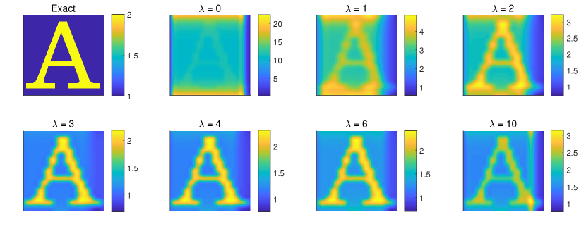
Figure 1: Test 1. The reconstructed coefficient $k(x)$, where the function $k(x)$ is given in (8.6) with $c_{a}=2$ inside of the letter ‘A’. We test different values of $\lambda$. The reconstructions are unsatisfactory when $\lambda$ is too small, $\lambda=0,1,2$. Next, the reconstruction quality is good when $\lambda=3,4$. On the other hand, the reconstruction quality deteriorates at $\lambda=10$. Thus, we choose $\lambda=3$ as the optimal value.

Test 2. We test the case when the inclusion in (8.6) has the shape of the letter ‘$A$’ for different values of the parameter $c_{a}=4,8$ inside of the letter ‘$A$’. Hence, by (8.7) the inclusion/background contrasts now are respectively $4:1$ and $8:1$. Computational results are displayed on Figure 2. One can observe that these images are accurate ones. In particular, the computed inclusion/background contrasts are accurate.

Figure 2: Test 2. Exact (left) and reconstructed (right) coefficient $k(x)$ with $c_{a}=4$ (first row) and $c_{a}=8$ (second row) inside of the letter ‘A’ as in (8.6). The inclusion/background contrasts in (8.7) are respectively $4:1$ and $8:1$. The reconstructions are accurate

Test 3. We test the case when the coefficient $k(x)$ in (8.6) has the shape of the letter ‘$\Omega$’ with $c_{a}=2$ inside of it. Results are presented on Figure 3. We again observe an accurate reconstruction.

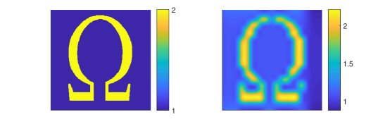
Figure 3: Test 3. Exact (left) and reconstructed (right) coefficient $k(x)$, where the function $k(x)$ is given in (8.6) with $c_{a}=2$ inside of the letter ‘$\Omega$’. The reconstruction is accurate.

Test 4. We now test different values of the parameter $c_{a}=4,8$ inside of the letter ‘$\Omega$’. The computational results are depicted on Figure 4. The quality of these images and computed inclusion/background contrasts in (8.7) are as good as the results of the test with the letter ‘$A$’ in Test 2.

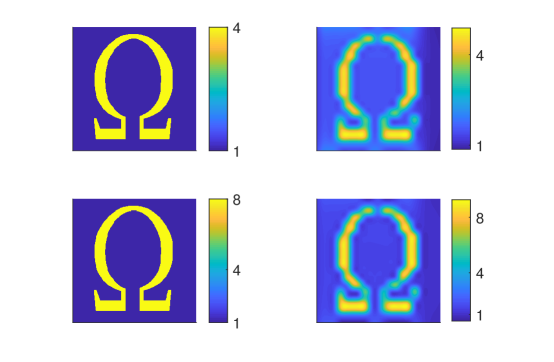
Figure 4: Test 4. Exact (left) and reconstructed (right) coefficient $k(x)$ with $c_{a}=4$ (first row) and $c_{a}=8$ (second row) inside of the letter ‘$\Omega$’ as in (8.6). The inclusion/background contrasts in (8.7) are respectively $4:1$ and $8:1$. The reconstructions are accurate.

Test 5. We test the reconstruction for the case when the inclusion in (8.6) has the shape of two letters ‘SZ’ with $c_{a}=2$ in each of them. SZ are two letters in the name of the city (Shenzhen) were the second and the third authors reside. The results are exhibited on Figure 5.

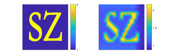
Figure 5: Test 5. Exact (left) and reconstructed (right) coefficient $k(x)$, where the function $k(x)$ is given in (8.6) with $c_{a}=2$ inside of two letters ‘SZ’. The reconstruction is worse than the one for the case of the single letter ‘$\Omega$’ in Figure 3. Nevertheless, the reconstruction are still accurate in both letters. The computed inclusion/background contrasts in (8.7) are accurately reconstructed in both letters.

Test 6. We consider the case of the random noisy data in (8.12) with $\delta=0.03$ and $\delta=0.05$, i.e. with 3% and 5% noise level. We test the reconstruction for the cases when the inclusion in (8.6) has the shape of either the letter ‘A’ or the letter ‘$\Omega$’ with $c_{a}=2$. The results are displayed on Figure 6. One can observe accurate reconstructions in all four cases. In particular, the inclusion/background contrasts in (8.7) are reconstructed accurately.

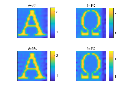
Figure 6: Test 6. Reconstructed coefficient $k(x)$ with the shape of letters ‘A’ (left) and ‘$\Omega$’ (right) with $c_{a}=2$ from noisy data (8.12) with $\delta=0.03$ (top) and $\delta=0.05$ (bottom), i.e. with 3% and 5% noise level. In all these four cases, both reconstructions and inclusion/background contrasts in (8.7) are accurate.

9 Summary

For the first time, we have developed here a numerical method for a CIP for MFGS (2.6) with the rigorously guaranteed global convergence property, see Definition 1.2 for the term “global convergence”. In other words, its convergence to the true solution is guaranteed if starting at an arbitrary point of a bounded set, whose diameter is not required to be small. We have proven the global convergence of our technique and explicitly provided its convergence rate.

To computationally demonstrate robustness of our technique, we took quite complicated shapes of tested inclusions. Our numerical results for both noiseless and noisy data demonstrate that we can accurately reconstruct both shapes of inclusions and values of the unknown coefficient both inside and outside of them.

References

References

- [1] Y. Achdou, P. Cardaliaguet, F. Delarue, A. Porretta, and F. Santambrogio. Mean Field Games, volume 2281 of Lecture Notes in Mathematics, C.I.M.E. Foundation Subseries. Springer Nature, Cetraro, Italy, 2019.
- [2] M. Asadzadeh and L. Beilina. Stability and convergence analysis of a domain decomposition FE/FD method for Maxwell’s equations in the time domain. Algorithms, 15:337, 2022.
- [3] M. Asadzadeh and L. Beilina. A stabilized P1 domain decomposition finite element method for time harmonic Maxwell’s equations. Math. Comput. Simul, 204:556–574, 2023.
- [4] A. B. Bakushinskii, M. V. Klibanov, and N. A. Koshev. Carleman weight functions for a globally convergent numerical method for ill-posed Cauchy problems for some quasilinear PDEs. Nonlinear Analysis: Real World Applications, 34:201–224, 2017.
- [5] L. Beilina and E. Lindstrom. An adaptive finite element/finite difference domain decomposition method for applications in microwave imaging. Electronics, 11:1359, 2022.
- [6] L. Beilina and V. Ruas. On the Maxwell-wave equation coupling problem and its explicit finite-element solution. Appl. Math., 68:75–98, 2022.
- [7] A. L. Bukhgeim and M. V. Klibanov. Uniqueness in the large of a class of multidimensional inverse problems. Soviet Math. Doklady, 17:244–247, 1981.
- [8] M. Burger, L. Caffarelli, and P. A. Markowich. Partial differential equation models in the socio-economic sciences. Philosophical Transactions of Royal Society, A372:20130406, 2014.
- [9] G. Chavent. Nonlinear Least Squares for Inverse Problems: Theoretical Foundations and Step-by-Step Guide for Applications. Springer Science & Business Media, New York, 2009.
- [10] Y. T. Chow, S. W. Fung, S. Liu, L. Nurbekyan, and S. Osher. A numerical algorithm for inverse problem from partial boundary measurement arising from mean field game problem. Inverse Probl., 39:014001, 2023.
- [11] R. Couillet, S. M. Perlaza, H. Tembine, and M. Debbah. Electrical vehicles in the smart grid: A mean field game analysis. IEEE J. Sel. Areas Commun., 30(6):1086–1096, 2012.
- [12] L. Ding, L. Li, S. Osher, and W. Yin. A mean field game inverse problem. J. Sci. Comput., 92:7, 2022.
- [13] G. Giorgi, M. Brignone, R. Aramini, and M. Piana. Application of the inhomogeneous Lippmann–Schwinger equation to inverse scattering problems. SIAM J. Appl. Math., 73:212–231, 2013.
- [14] A. V. Goncharsky and S. Y. Romanov. Iterative methods for solving coefficient inverse problems of wave tomography in models with attenuation. Inverse Probl., 33:025003, 2017.
- [15] A. V. Goncharsky and S. Y. Romanov. A method of solving the coefficient inverse problems of wave tomography. Comput. Math. Appl., 77:967–980, 2019.
- [16] M. Huang, P. E. Caines, and R. P. Malhamé. Large-population cost-coupled LQG problems with nonuniform agents: individual-mass behavior and decentralized Nash equilibria. IEEE Trans. Automat. Control, 52:1560–1571, 2007.
- [17] M. Huang, R. P. Malhamé, and P. E. Caines. Large population stochastic dynamic games: closed-loop McKean-Vlasov systems and the Nash certainty equivalence principle. Commun. Inf. Syst., 6:221–251, 2006.
- [18] M. V. Klibanov. Global convexity in a three-dimensional inverse acoustic problem. SIAM J. Math. Anal., 28:1371–1388, 1997.
- [19] M. V. Klibanov and A. Timonov. Carleman Estimates for Coefficient Inverse Problems and Numerical Applications. VSP, Utrecht, 2004.
- [20] M. V. Klibanov. Carleman estimates for global uniqueness, stability and numerical methods for coefficient inverse problems. J. Inverse Ill-Posed Probl., 21:477–510, 2013.
- [21] M.V. Klibanov, J. Li, and W. Zhang. Convexification for an inverse parabolic problem. Inverse Probl., 36:085008, 2020.
- [22] M. V. Klibanov, V. A. Khoa, A. V. Smirnov, L. H. Nguyen, G. W. Bidney, L. Nguyen, A. Sullivan, and V. N. Astratov. Convexification inversion method for nonlinear SAR imaging with experimentally collected data. J. Appl. Ind. Math., 15:413–436, 2021.
- [23] M. V. Klibanov and J. Li. Inverse Problems and Carleman Estimates: Global Uniqueness, Global Convergence and Experimental Data. De Gruyter, Berlin, 2021.
- [24] M. V. Klibanov and Y. Averboukh. Lipschitz stability estimate and uniqueness in the retrospective analysis for the mean field games system via two Carleman estimates. SIAM J. Math. Anal., 2023.
- [25] M. V. Klibanov. The mean field games system: Carleman estimates, Lipschitz stability and uniqueness. J. Inverse Ill-Posed Probl., published online, 2023.
- [26] M. V. Klibanov, J. Li, and H. Liu. Hölder stability and uniqueness for the mean field games system via Carleman estimates. Studies in Applied Mathematics, pages 1–24, 2023.
- [27] M. V. Klibanov, J. Li, and H. Liu. Coefficient inverse problems for a generalized mean field games system with the final overdetermination. arXiv:2305.01065, 2023.
- [28] M. V. Klibanov. A coefficient inverse problem for the mean field games system. Appl. Math. Optim., 88:54, 2023.
- [29] M. V. Klibanov, J. Li, and Z. Yang. Convexification numerical method for the retrospective problem of mean field games. arXiv:2306.14404, 2023.
- [30] V. N. Kolokoltsov and O. A. Malafeyev. Many Agent Games in Socio-economic Systems: Corruption, Inspection, Coalition Building, Network Growth, Security. Springer Nature Switzerland AG, 2019.
- [31] J.-M. Lasry and P.-L. Lions. Jeux à champ moyen. i. le cas stationnaire. C. R. Math. Acad. Sci. Paris, 343:619–625, 2006.
- [32] J.-M. Lasry and P.-L. Lions. Mean field games. Japanese Journal of Mathematics, 2:229–260, 2007.
- [33] T. T. Le and L. H. Nguyen. The gradient descent method for the convexification to solve boundary value problems of quasi-linear PDEs and a coefficient inverse problem. J. Sci. Comput., 91(3):74, 2022.
- [34] H. Liu, C. Mou, and S. Zhang. Inverse problems for mean field games. Inverse Probl., 39:085003, 2023.
- [35] H. Liu and S. Zhang. On an inverse boundary problem for mean field games. arXiv:2212.09110, 2022.
- [36] H. Liu and S. Zhang. Simultaneously recovering running cost and Hamiltonian in mean field games system. arXiv:2303.13096, 2023.
- [37] S. Liu, M. Jacobs, W. Li, L. Nurbekyan, and S. Osher. Computational methods for first order nonlocal mean field games with applications. SIAM J. Numer. Anal., 59:2639–2668, 2021.
- [38] R. G. Novikov. The approach to approximate inverse scattering at fixed energy in three dimensions. International Math. Research Peports, 6:287–349, 2005.
- [39] G. Rizutti and A. Gisolf. An iterative method for 2D inverse scattering problems by alternating reconstruction of medium properties and wavelets: theory and application to the inversion of elastic waveforms. Inverse Probl., 33:035003, 2017.
- [40] V. G. Romanov. Inverse Problems of Mathematical Physics. VNU Press, Utrecht, The Netherlands, 1987.
- [41] J. A. Scales, M. L. Smith, and T. L. Fischer. Global optimization methods for multimodal inverse problems. J. Comp. Phys., 103:258–268, 1992.
- [42] A. N. Tikhonov, A. V. Goncharsky, V. V. Stepanov, and A. G. Yagola. Numerical methods for the solution of Ill-posed problems. Kluwer, London, 1995.
- [43] N. V. Trusov. Numerical study of the stock market crises based on mean field games approach. J. Inverse Ill-Posed Probl., 29:849–865, 2021.