Estimation of the Characteristic Wavelength Parameter in 1D Leray-Burgers Equation with PINN

Abstract

In this paper, we employ the Physics-Informed Neural Network (PINN) to estimate the practical range of the characteristic wavelength parameter (referred to as the smoothing parameter) $\alpha$ in the Leray-Burgers equation. The Leray-Burgers equation, a regularization of the inviscid Burgers equation, incorporates a Helmholtz filter with a characteristic wavelength $\alpha$ to replace the usual convective velocity inducing a regularized convective velocity. The filter bends the equation’s characteristics slightly and makes them not intersect each other, leading to a global solution in time. By conducting computational experiments with various initial conditions, we determine the practical range of $\alpha>0$ that closely approximates the solutions of the inviscid Burgers equation. Our findings indicate that the value of $\alpha$ depends on the initial data, with the practical range of $\alpha$ being between 0.01 and 0.05 for continuous initial profiles and between 0.01 and 0.03 for discontinuous initial profiles. The Leray-Burgers equation captures shock and rarefaction waves within the temporal domain for which training data exists. However, as the temporal domain extends beyond the training interval, data-driven forward computation demonstrates that the predictions generated by the PINN start to deviate from the exact solutions. This study also highlights the effectiveness and efficiency of the Leray-Burgers equation in real practical problems, specifically Traffic State Estimation.

1 Introduction

We consider a problem of computing the solution $v:[0,T]\times\Omega\to\mathbb{R}$ of an evolution equation

$$v_{t}(t,x)+\mathcal{N}_{\alpha}\,[v](t,x)=0, \forall(t,x)\in(0,T]\times\Omega,$$ (1.1)

$$v(0,x)=v_{0}(x)\quad \forall x\in\Omega,$$ (1.2)

where $\mathcal{N}_{\alpha}$ is a nonlinear differential operator acting on $v$ with a small constant parameter $\alpha>0$,

$$\mathcal{N}_{\alpha}[v]=vv_{x}+\alpha^{2}v_{x}v_{xx}.$$ (1.3)

Here the subscripts of $v$ mean partial derivatives in $t$ and $x$, $\Omega\subset\mathbb{R}$ is a bounded domain, $T$ denotes the final time and $v_{0}:\Omega\to\mathbb{R}$ is the prescribed initial data. Although the methodology allows for different types of boundary conditions, we restrict our discussion to Dirichlet or periodic cases and prescribe the boundary data as

$$v_{b}(t,x)=v(t,x),\quad\forall(t,x)\in(0,T]\times\partial\Omega,$$ (1.4)

where $\partial\Omega$ denotes the boundary of the domain $\Omega$.

The equation (1.1) is called the Leray-Burgers equation. It is also known as Burgers-$\alpha$, or connectively filtered Burgers equation, etc., in literature. Bhat and Fetecau [2] introduced (1.1) as a regularized approximation to the inviscid Burgers equation

$$v_{t}+vv_{x}=0.$$ (1.5)

They considered a special smoothing kernel associated with the Green function of the Helmholtz operator

$$u_{\alpha}=\mathcal{H}^{-1}_{\alpha}v=(I-\alpha^{2}\partial_{x}^{2})^{-1}v,\ \ (I=identity),$$

where $\alpha>0$ is interpreted as the characteristic wavelength scale below which the smaller physical phenomena are averaged out (see for example [9]). Applying the smoothing kernel to the convective term in (1.5) yields

$$v_{t}+u_{\alpha}v_{x}=0,$$ (1.6)

where $v=v(t,x)$ is a vector field and $u_{\alpha}$ is the filtered vector field. The filtered vector $u_{\alpha}$ is smoother than $v$ and the equation (1.6) is a nonlinear Leray-type regularization [14] of the inviscid Burgers equation. Here and in the following, we abuse the notation of the filtered vector $u_{\alpha}$ with $u$. If we express the equation (1.6) in the filtered vector $u$, it becomes a quasilinear evolution equation that consists of the inviscid Burgers equation plus $\mathcal{O}(\alpha^{2})$ nonlinear terms [2, 3, 4]:

$$u_{t}+uu_{x}=\alpha^{2}(u_{txx}+uu_{xxx}).$$ (1.7)

In this paper, we follow Zhao and Mohseni [23] to expand the inverse Helmholz operator in $\alpha$ to higher orders of the Laplacian operator:

$$(1-\alpha^{2}\Delta)^{-1}=1+\alpha^{2}\Delta+\alpha^{4}\Delta^{2}+\cdots\ \mbox{if}\ \alpha\lambda_{\mathrm{max}}<1,$$

where $\lambda_{\mathrm{max}}$ is the highest eigenvalue of the discretized operator $\Delta$. Then we can write (1.6) in the unfiltered vector fields $v$ to get the equation (1.1)-(1.3) with $\mathcal{O}(\alpha^{4})$ truncation error.

For smooth initial data $v(0,x)$ decreasing at least at one point (so there exists $y$ such that $v_{x}(0,y)<0$), the classical solution $v(t,x)$ of the inviscid Burgers equation (when $\alpha=0$) fails to exist beyond a specific finite break time $T_{s}>0$. It is because the characteristics of the inviscid equation intersect in finite time. The Leray-Burgers equation bends the characteristics to make them not intersect each other, avoiding any finite-time intersection and remedying the finite-time breakdown [2, 4]. So, the Leray-Burgers equation possesses a classical solution globally in time for smooth initial data for $\alpha>0$ [2]:

Theorem 1.

Given initial data $v_{0}\in W^{2,1}(\mathbb{R})=\{u\in L^{1}(\mathbb{R}):D^{s}u\in L^{1}(\mathbb{R})\ \ \mathrm{for\ all}\ \ |s|\leq 2\}$, the Leray-Burgers equation (1.6) possesses a unique solution $v(t,x)\in W^{2,1}(\mathbb{R})$ for all $t>0$.

Furthermore, the Leray-Burgers solution $u_{\alpha}(t,x)$ with initial data $u_{\alpha}(0,x)=\mathcal{H}^{-1}_{\alpha}v_{0}(x)$ for $v_{0}\in W^{2,1}(\mathbb{R})$ converges strongly, as $\alpha\rightarrow 0^{+}$, to a global weak solution $v(t,x)$ of the following initial-value problem for the inviscid Burgers equation (Theorem 2 in [2]):

$$v_{t}+\frac{1}{2}\left(v^{2}\right)_{x}=0\ \ \ \mbox{with}\ \ v(0,x)=v_{0}(x).$$ (1.8)

Bhat and Fetecau [2] found numerical evidence that the chosen weak solution in the zero-$\alpha$ limit satisfies the Oleinik entropy inequality, making the solution physically appropriate. The proof relies on the uniform estimates of the unfiltered velocity $v$ rather than the filtered velocity $u$. It made possible the strong convergence of the Leray-Burgers solution to the correct entropy solution of the inviscid Burgers equation. In the context of the filtered velocity $u_{\alpha}$, they also showed that the Leray-Burgers equation captures the correct shock solution of the inviscid Burgers equation for Riemann data consisting of a single decreasing jump [4]. However, since $u_{\alpha}$ captures an unphysical solution for Riemann data comprised of a single increasing jump, it was necessary to control the behavior of the regularized equation by introducing an arbitrary mollification of the Riemann data to capture the correct rarefaction solution of the inviscid Burgers equation. With that modification, they extended the existence results to the case of discontinuous initial data $u_{\alpha}\in L^{\infty}$. But, it is still an open problem for initial data $v_{0}\in L^{\infty}$. In [7], Guelmame, et all, derived a similar regularized equation to (1.7):

$$u_{t}+uu_{x}=\alpha^{2}(u_{txx}+2u_{x}u_{xx}+uu_{xxx}),$$ (1.9)

which has an additional term $2u_{x}u_{xx}$ on the right-handed side. Notice that $u$ in this equation is the filtered vector field in (1.6). When they were establishing the existence of the entropy solution, Guelmame, et all. resorted to altering the equation (1.9), as Bhat and Fetecau had to modify the initial data for their proof in [4]. Analysis in the context of the filtered vector field $u$ appears to induce additional modification of the equations to achieve the desired results. Working with the actual vector field $v$ may avoid such arbitrary changes. Equation (1.6) and related models have previously appeared in the literature. We refer [1, 2, 3, 4, 6, 7, 16, 22, 20] for more properties related to the Leray-Burgers equation.

One question remains open. How do we choose the parameter $\alpha$? The link between regularization procedures such as Helmholtz regularization and numerical schemes had been studied before, for example in [6, 16]. Gottwald [6] argued that, in numerical computations, the parameter $\alpha^{2}$ cannot be interpreted solely as a length scale because it also depends on the numerical discretization scheme chosen. One practical rule of thumb is to choose $\alpha$ as some small integer multiple of the minimum grid spacing. Pavlova [16] also conducted numerical experiments in determining physically reasonable choices of $\alpha$ based on the conservation of total mass in time. Their finding is that, for a fixed mesh size $h$, as the number of space grids $N$ increases, the $\alpha$ decreases. Also, for a fixed $N$, there is a particular value of $\alpha\approx 0.02$ below which the solution becomes oscillatory (even with continuous initial profiles), violating maximum conservation condition. In the context of Burgers equation, $\alpha=0.4,0.3,0.2,0.0327,0.0216,..$ were used depending on a relation between $\alpha$ and the mesh size that preserves stability and consistency with conservation conditions for the chosen numerical scheme [2, 6, 16]. Here we use the physics-informed neural network [17, 18] to estimate the range of values of $\alpha$ closely approximating the exact Burgers equation and simulate the learned new Leray-Burgers equation to compare with the original Burgers equation. We will also demonstrate that it correctly captures physical shocks by solving the Riemann problems.

The results show that the $\alpha$ value depends on the initial data, with the practical range of $\alpha$ being between 0.01 and 0.05 for continuous initial profiles and between 0.01 and 0.03 for discontinuous initial profiles (Section 4). We also note that the Leray-Burgers equation written in the filtered vector $u$ does not appear to produce reliable estimates of $\alpha$. Approximating the solution $u$ with relatively good accuracy requires significantly more training data points than in $v$, and the range of $\alpha$-values for $u$ solutions is narrower, between 0.0001 and 0.005, than the $\alpha$ range for $v$ (Section 6). Nevertheless, the Multilayer Perceptron-based PINN (MLP-PINN) struggled to converge to the Burgers solutions in the context of the filtered vector field $u$. We may say that the equation written in the unfiltered vector field $v$ is a better approximation to the exact Burgers equation.

In Section 7, we assess the validity of the $\alpha$-values by solving some initial-value problems with an MLP-PINN (forward inference). We observe that the MLP-PINN generates spurious oscillations near discontinuities in shock-producing initial profiles, which prevents the PINN solution from converging to an exact inviscid Burgers solution as $\alpha\rightarrow 0^{+}$.

Also, in Section 7, we illustrate a limitation of the MLP-PINN in accurately predicting solutions beyond the designated temporal domain for training. Our empirical experiments show that, as the temporal domain progresses beyond the training interval, the predictions with the MLP-PINN begins to deviate from the exact solutions.

In Section 8, we present a brief investigation of two variants of the Lighthill-Whitham-Richards (LWR) traffic flow model, namely LWR-$\alpha$ (based on the Leray-Burgers equation) and LWR-$\epsilon$ (based on the viscous Burgers equation), in the context of Traffic State Estimation (TSE). The result demonstrates the efficacy of the LWR-$\alpha$ model as a suitable alternative for traffic state estimation, outperforming the diffusion-based LWR-$\epsilon$ model in terms of computational efficiency.

2 Problem Formulation

We set up the computational frame for the governing system (1.1) by

$$v_{t}+\lambda_{1}vv_{x}+\lambda_{2}v_{x}v_{xx}=0,\ \ t\in[0,T],\ x\in\Omega$$ (2.1)

$$v(0,x)=f(x),\ x\in\Omega\hskip 36.135pt$$ (2.2)

$$v(t,x)=g(t,x),\ t\in[0,T],\ x\in\partial\Omega,\hskip 7.22743pt$$ (2.3)

where $\Omega\subset\mathcal{R}$ is a bounded domain, $\partial\Omega$ is a boundary of $\Omega$, $f(x)$ is an initial distribution, and $g(t,x)$ is a boundary data. We intentionally introduced a new parameter $\lambda_{1}$ and set $\lambda_{2}=\alpha^{2}$. During the training process, the PINN will learn $\lambda_{1}$ to determine the validity of the obtained $\alpha$ for the inviscid Burgers equation ($\lambda=1$) along with the relative errors. We use numerical or analytical solutions of the exact inviscid and viscous Burgers equations to generate training data sets $D$ with different initial and boundary conditions:

$$D=\left\{(t_{i},x_{i},v_{i}),\ i=1,...,N_{d}\right\},$$

where $v_{i}=v(t_{i},x_{i})$ denotes the output value at position $x_{i}\in\Omega$ and time $0<t_{i}\leq T$ with the final time $T$. $N_{d}$ refers to the number of training data. Our goal is to estimate the effective range of $\alpha$ such that the neural network $v_{\theta}$ satisfies the equation (2.1)-(2.3) and $v_{\theta}(t_{i},x_{i})\approx v_{i}$. The training models selected represent a range of initial conditions, from continuous initial data to discontinuous data, displaying both shock and rarefaction waves.

3 Methodology

Following the original work of Raissi et al. [17, 18], we use a Physics-Informed Neural Network (PINN) to determine physically meaningful $\alpha$-values closely approximating the entropy solutions to the inviscid Burgers equation. The basic architecture of the PINN is the integration of a neural network with physical knowledge of the dynamics of interests through the inclusion of the associated mathematical model, both sharing hyperparameters and contributing to a loss function.

\begin{overpic}[width=390.25534pt,tics=8]{./img/Flow_Diagram1.png} \end{overpic}

Figure 1: The PINN Diagram

The underlying neural network for our problem (Figure 1) is a fully connected feed-forward neural network, known as a multilayer perceptron (MLP). The PINN enforces the physical constraint,

$$\mathcal{F}(t,x)\coloneq v_{t}+\lambda_{1}vv_{x}+\lambda_{2}v_{x}v_{xx}$$

on the MLP surrogate $v_{\theta}(t,x;\xi)$, where $\theta=\theta(W,b)$ denotes all parameters of the network (weights $W$ and biases $b$) and $\xi=(\lambda_{1},\lambda_{2})$ the physical parameters in (2.1), acting directly in the loss function

$$\mathcal{L}(\theta,\xi)=\mathcal{L}_{d}(\theta,\xi)+\mathcal{L}_{r}(\theta,\xi),$$ (3.1)

where $\mathcal{L}_{d}$ is the loss function on the available measurement data set that consists in the mean-squared-error (MSE) between the MLP’s predictions and training data and $\mathcal{L}_{r}$ is the additional residual term quantifying the discrepancy of the neural network surrogate $v_{\theta}$ with respect to the underlying differential operator in (2.1). We define the data residual

$$\mathcal{R}_{d,\theta}(t_{i},x_{i};\xi_{i})\coloneq v_{\theta}(t_{i},x_{i};\xi_{i})-v(t_{i},x_{i}),\ \ \forall(t_{i},x_{j})\in D$$ (3.2)

and the PDE residual:

$$\mathcal{R}_{r,\theta}(t_{i},x_{i};\xi_{i})\coloneq\partial_{t}v_{\theta}+\lambda_{1}v_{\theta}\partial_{x}v_{\theta}+\lambda_{2}\partial_{x}v_{\theta}\partial_{xx}v_{\theta},\ \ \forall(t_{i},x_{j})\in D,$$ (3.3)

where $\{t_{i},x_{i}\}_{i=1}^{N_{d}}$ is the set of the coordinates of training data in $D$ and $v_{\theta}=v_{\theta}(t_{i},x_{i};\xi_{i})$. Then, the data loss and residual loss functions in (3.1) can be written as

$$\mathcal{L}_{d}(\theta,\xi) = \frac{1}{N_{d}}\sum_{i=1}^{N_{d}}\Big{|}\mathcal{R}_{d,\theta}(t_{i},x_{i};\xi_{i})\Big{|}^{2}$$ (3.4)

$$\mathcal{L}_{r}(\theta,\xi) = \frac{1}{N_{d}}\sum_{i=1}^{N_{d}}\Big{|}\mathcal{R}_{r,\theta}(t_{i},x_{i};\xi_{i})\Big{|}^{2}.$$ (3.5)

The goal is to find the network and physical parameters $\theta$ and $\xi$ minimizing the loss function (3.1):

$$(\theta^{*},\xi^{*})=\underset{\theta\in\Theta,\xi\in\Xi}{\arg\min}\,\mathcal{L}(\theta,\xi)$$ (3.6)

over an admissible sets $\Theta$ and $\Xi$ of training network parameters $\theta$ and $\xi$, respectively.

In practice, given the set of scattered data $v_{i}=v(t_{i},x_{i})$, the MLP takes the coordinate $(t_{i},x_{i})$ as inputs and produces output vectors $v_{\theta}(t_{i},x_{i};\xi_{i})$ that has the same dimension as $v_{i}$. The PDE residual $\mathcal{R}_{r,\theta}(x,t;\xi)$ forces the output vector $v_{\theta}$ to comply with the physics imposed by the Leray-Burgers equation. The PDE residual network takes its derivatives with respect to input variables $x$ and $t$ by applying the chain rule for differentiating compositions of functions using the automatic differentiation integrated into TensorFlow. The residual of the underlying differential equation is evaluated using these gradients. The data loss and the physics loss are trained using inputs from across the entire domain of interest. The physics loss does not require target values, as it is designed to incorporate knowledge about the physical laws that govern the system being modelled. Therefore, any appropriate sampling strategy can be employed to generate inputs for the physics loss. Some common sampling strategies include uniform sampling, space-filling Latin hypercube sampling, and random sampling.

4 Experiment 1: Inviscid with Riemann Initial Data

We consider the inviscid Burgers equation (1.5) with some standard Riemann initial data of the form

$$v_{0}(x) = \left\{\begin{array}[]{cc}v_{L},&x\leq 0\\ v_{M},&0<x\leq 1\\ v_{R},&x>1\end{array}\right.$$ (4.4)

We used the conservative upwind difference scheme to generate training data. For each initial profile, we computed $256\times 101=25856$ data points through the entire spatio-temporal domain. We modified the code in [18] and, for each case, we performed ten computational simulations with 2000 training data randomly sampled for each computation. We adopted the Limited-Memory BFGS (L-BFGS) optimizer with a learning rate of 0.01 to minimize the mean square error loss (3.1). When the L-BFGS optimizer diverged, we preprocessed with the ADAM optimizer and finalized the optimization with the L-BFGS. We manually checked with random sets of hyperparameters by training the algorithm and selected the best set of parameters that fits our objective, 8-hidden-layers and 20 units per layer, $10000$ epochs. We trained the other models with the same parameters, which might not be the best but reasonable fit for them. One remark is that our problem is identifying the model parameter $\alpha$ rather than inferencing solutions, and it is unnecessary to consider the physical causality in our loss function (3.1) as pointed out in [21].

Upon training, the network is calibrated to predict the entire solution $v(t,x)$, as well as the unknown parameters $\theta$ and $\xi$. Along with the relative $L^{2}$-norm of the difference between the exact solution and the corresponding trial solution

$$\ell^{2}_{error}(v_{\theta}):=||v-v_{\theta}||_{2}/||v||_{2},$$ (4.5)

we used the absolute error of $\lambda_{1}$, $\epsilon(\lambda_{1})=|1-\lambda_{1}|$ in determining the validity of each computational result. The results show that the $\alpha$ value depends on the initial data, with the effective range of $\alpha$ being between 0.01 and 0.05 for continuous initial profiles and between 0.01 and 0.03 for discontinuous initial profiles. The results show that the equation adequately develops the shock with a relative error of about $10^{-2}$. We present some examples in the following subsections.

4.1 Shock Waves

We consider two different initial profiles that develop shocks:

$$v_{t}+vv_{x}=0,\ x\in\mathbb{R},\ t\in[0,1)\ \ \mathrm{with\ the\ initial\ data}\hskip 93.95122pt$$ (4.6)

$$\mathrm{(I)}\ \ v(0,x)=\left\{\begin{array}[]{cl}1&\mbox{if}\ x\leq 0\\ 1-x&\mbox{if}\ 0<x<1\\ 0&\mbox{if}\ x\geq 1\end{array}\right.\ \ \mathrm{or}\ \ \mathrm{(II)}\ \ v(0,x)=\left\{\begin{array}[]{cl}1&\mbox{if}\ x\leq 0\\ 0&\mbox{if}\ x>0.\end{array}\right.$$ (4.12)

The exact entropy solutions corresponding to the initial data (I) and (II) in (4.12) are

$$\mathrm{(I^{\prime})}\ \ v(t,x)=\left\{\begin{array}[]{cl}1&\mbox{if}\ x\leq t\\ \frac{1-x}{1-t}&\mbox{if}\ t<x<1\\ 0&\mbox{if}\ x\geq 1\end{array}\right. \mathrm{and} \mathrm{(II^{\prime})}\ \ v(t,x)=\left\{\begin{array}[]{cl}1&\mbox{if}\ x\leq\frac{t}{2}\\ 0&\mbox{if}\ x>\frac{t}{2},\end{array}\right.$$ (4.18)

respectively. The initial profile (I) in (4.12) represents a ramp function with a slope of $-1$, which creates a wave that travels faster on the left-hand side of $x$ than on the right-hand side. The faster wave overtakes the slow wave, causing a discontinuity when $t=1$, as we can see from the exact solution $\mathrm{(I^{\prime})}$ in (4.18). The second initial data (II) in (4.12) contains a discontinuity at $x=0$. Its solution needs a shock fitting just from the beginning. Based on the Rankine-Hugoniot condition, the discontinuity must travel at speed $x^{\prime}(t)=\frac{1}{2}$, which we can observe in the analytical solution $\mathrm{(II^{\prime})}$ in (4.18). The solution also satisfies the entropy condition, which guarantees that it is the unique weak solution for the problem. Table 1 shows ten computational results.

No.	Initial Profile (I)			Initial Profile (II)
	$\lambda_{2}=\alpha^{2}$	$\epsilon(\lambda_{1})$	$\ell^{2}$ Error	$\lambda_{2}=\alpha^{2}$	$\epsilon(\lambda_{1})$	$\ell^{2}$ Error
1	0.0011137	0.0034	5.73e-03	0.000676	0.0618	7.16e-03
2	0.0012754	0.0066	5.91e-03	0.0004459	0.0232	3.70e-03
3	0.0015410	0.0124	5.17e-03	0.0004853	0.0170	5.31e-03
4	0.0013057	0.0133	5.62e-03	0.0005689	0.0072	5.92e-03
5	0.0014716	0.0062	5.45e-03	0.0006529	0.0065	7.77e-03
6	0.0013240	0.0061	5.09e-03	0.0008408	0.0204	1.04e-02
7	0.0006021	0.0103	7.02e-03	0.0008763	0.0591	1.09e-02
8	0.0019446	0.0067	5.29e-03	0.0008772	0.0045	1.23e-02
9	0.0007324	0.0056	6.36e-03	0.0009172	0.0151	1.76e-02
10	0.0018084	0.0124	5.33e-03	0.0007642	0.0004	9.83e-03
Average	$0.0013119$	0.0083	5.70e-03	$0.0007105$	0.0212	9.09e-03
	$\alpha=0.0362$			$\alpha=0.0267$

Table 1: Ten computational simulation results with $N_{d}=2000$ training data randomly sampled for each computation.

In both cases, the $\epsilon(\lambda_{1})$ is within $10^{-2}$ and $10^{-1}$, indicating that the inferred PDE residual reflects the actual Leray-Burgers equations within an acceptable range. The average value of $\alpha$ with the initial profile (I) was $0.0362$ with a relative error of $5.7\times 10^{-3}$. Figure 2 shows a plot example. We can see the Leray-Burgers solution well captures the shock wave and maintains the discontinuity at $x=1$ as $t$ evolves to $1$. Computations with the initial profile (II) resulted in $\alpha\approx 0.0267$ on average with a relative error $9.1\times 10^{-3}$. Figure 2 shows that the Leray-Burgers equation captures the shock wave as well as its speed $\frac{1}{2}$ per unit time. Increasing the training data ($N_{d}\geq 4000$) did not change the value of $\alpha$ significantly.

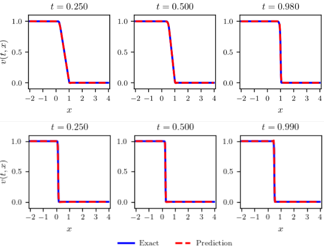
Figure 2: Top: Evolution with the initial profile (I) with $\alpha\approx 0.0334$, $\epsilon(\lambda_{1})\approx 0.0034$, and $\epsilon(\ell^{2})\approx 5.73\times 10^{-3}$. Bottom: Evolution with the initial profile (II) with $\alpha\approx 0.0276$, $\epsilon(\lambda_{1})\approx 0.0004$, and $\epsilon(\ell^{2})\approx 9.83\times 10^{-3}$.

4.2 Rarefaction Waves

We generate a training data set from the following inviscid Burgers equation and an initial condition:

$$v_{t}+vv_{x}=0,\ x\in\mathbb{R},\ t\in[0,2]\ \ \mathrm{with\ the\ initial\ data}\hskip 93.95122pt$$ (4.19)

$$\mathrm{(III)}\ \ v(0,x)=\left\{\begin{array}[]{cl}0&\mbox{if}\ x\leq 0\\ x&\mbox{if}\ 0<x<1\\ 1&\mbox{if}\ x\geq 1\end{array}\right.\ \ \mathrm{or}\ \ \mathrm{(IV)}\ \ v(0,x)=\left\{\begin{array}[]{cl}0&\mbox{if}\ x\leq 0\\ 1&\mbox{if}\ x>0.\end{array}\right.$$ (4.25)

The rarefaction waves are continuous self-similar solutions, which are

$$\mathrm{(III^{\prime})}\ \ v(t,x)=\left\{\begin{array}[]{cl}0&\mbox{if}\ x\leq 0\\ \frac{x}{1+t}&\mbox{if}\ 0<x<1+t\\ 1&\mbox{if}\ x\geq 1+t\end{array}\right. \mathrm{and} \mathrm{(IV^{\prime})}\ \ v(t,x)=\left\{\begin{array}[]{cl}0&\mbox{if}\ x\leq 0\\ \frac{x}{t}&\mbox{if}\ 0<x<t\\ 1&\mbox{if}\ x\geq t\end{array}\right.$$

corresponding to the initial data (III) and (IV) in (4.25), respectively.

In both cases, the $\epsilon(\lambda_{1})$ is within $10^{-2}$, indicating that the inferred PDE residual reflects the actual Leray-Burgers equations within an acceptable range. The average value of $\alpha$ are $0.0488$ with a relative error of $1.99\times 10^{-3}$ with the continuous initial profile (III) and $\alpha\approx 0.0276$ with a relative error of $7.5\times 10^{-3}$ with the discontinuous initial profile (IV). Figure 3 shows that the Leray-Burgers equation captures the rarefaction waves well.

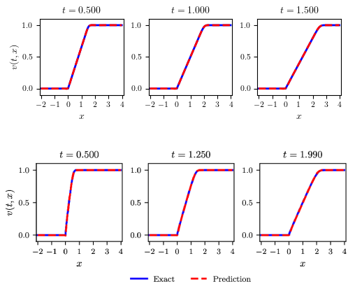
Figure 3: Top: Evolution with the initial profile (III). Bottom: Evolution with the initial profile (IV).

4.3 Shock and Rarefaction Waves

We combine the shock and rarefaction waves:

$$v_{t}+vv_{x}=0,\ x\in\mathbb{R},\ t\in[0,2]\ \ \mathrm{with\ the\ initial\ data,}\hskip 93.95122pt$$ (4.27)

$$\mathrm{(V)}\ \ v(0,x)=\left\{\begin{array}[]{cc}0&\mbox{if}\ x\leq-1\\ 1+x&\mbox{if}\ -1<x\leq 0\\ 1-x&\mbox{if}\ 0<x\leq 1\\ 0&\mbox{if}\ x>1\end{array}\right.\ \ \mathrm{or}\ \ \mathrm{(VI)}\ \ v(0,x)=\left\{\begin{array}[]{cc}0&\mbox{if}\ x<0\\ 1&\mbox{if}\ 0\leq x\leq 1\\ 0&\mbox{if}\ x>1\end{array}\right.$$ (4.35)

In both cases, the $\epsilon(\lambda_{1})$ is within $10^{-2}$, indicating that the inferred PDE residual reflects the actual Leray-Burgers equations within an acceptable range. The average value of $\alpha$ are $0.0348$ with a relative error of $1.95\times 10^{-2}$ with the continuous initial profile (V) and $\alpha\approx 0.0316$ with a relative error of $\ell^{2}\approx 3.17\times 10^{-2}$ with the discontinuous initial profile (VI). Figure 4 shows that the Leray-Burgers equation captures both shock and rarefaction waves well.

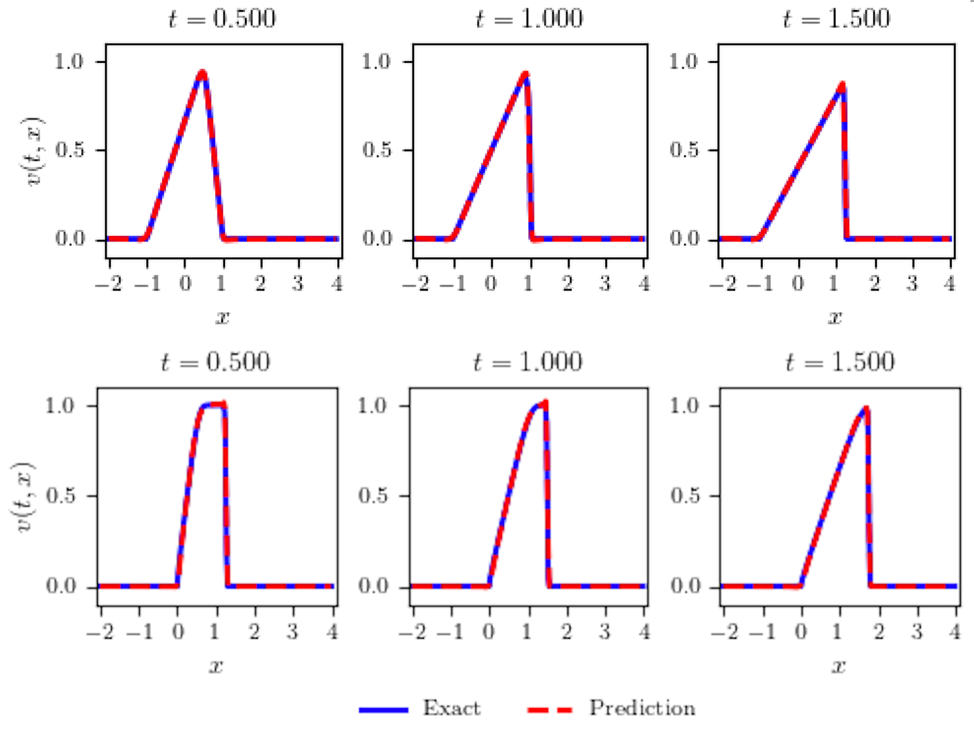
Figure 4: Top: Evolution with the initial profile (V). Bottom: Evolution with the initial profile (VI).

4.4 One Hump

Another interesting case is one-hump initial condition:

$$v_{t}+vv_{x}=0,x\in\mathbb{R},\ t\in[0,2],\hskip 21.68121pt$$

$$v(0,x)=e^{-0.5(x/0.4)^{2}}.\quad\quad\quad$$

The $\epsilon(\lambda_{1})$ is within $10^{-2}$, indicating that the inferred PDE residual reflects the actual Leray-Burgers equations within an acceptable range. The average value of $\alpha$ is $0.0381$ with the relative error of $2.24\times 10^{-2}$ (Figure 5).

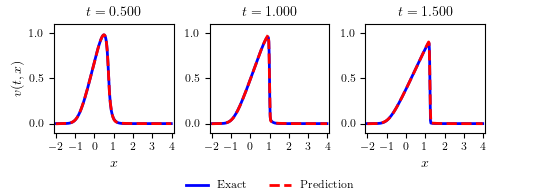
Figure 5: Evolution with a one-hump initial profile.

5 Experiment 2: Viscid Cases

In this section, we consider the following viscous Burgers equation for a training data set:

$$v_{t}+vv_{x}=\nu v_{xx},\ \ \ \forall(t,x)\in(0,T]\times\Omega\hskip 130.08621pt$$ (5.1)

$$\mathrm{(A)}\ \ \left\{\begin{array}[]{cc}\nu=\frac{0.01}{\pi},\ T=1,\Omega=(-1,1)&\\ v(0,x)=-\sin(\pi x),\ \forall x\in[-1,1]&\\ v(t,-1)=v(t,1)=0,\ \forall t\in[0,1]\end{array}\right.\ \ \mathrm{or}\ \ \mathrm{(B)}\ \ \left\{\begin{array}[]{cc}\nu=0.07,\ T\approx 0.4327,\ \Omega=[0,2\pi]&\\ v(0,x)=-2\nu\frac{\phi^{\prime}}{\phi}+4,&\\ \phi(x)=\exp\left(\frac{-x^{2}}{4\nu}\right)+\exp\left(\frac{-(x-2\pi)^{2}}{4\nu}\right).\end{array}\right.$$ (5.8)

The corresponding $\alpha$ equation is

$$v_{t}+vv_{x}=-\alpha^{2}v_{x}v_{xx}.$$

For the initial and boundary data (A), Rudy, et all, [19] proposed the data set which can correctly identify the viscous Burgers equation solely from time-series data. It contains 101-time snapshots of a solution to the Burgers equation with a Gaussian initial condition propagating into a traveling wave. Each snapshot has 256 uniform spatial grids. For our experiment, we adopt the data set prepared by Raissi, et all, in [17, 18] based on [19], $101\times 256=25856$ data points, generated from the exact solution to (5.1). For training, $N_{d}=2000$ collocation points are randomly sampled and we use L-BFGS optimizer with a learning rate of 0.8. The average over ten experiments is $\alpha=0.0158$ with $\ell^{2}_{error}(v_{\theta})\approx 3.8\times 10^{-2}$. The computational simulation shows the equation develops a shock properly (Figure 6).

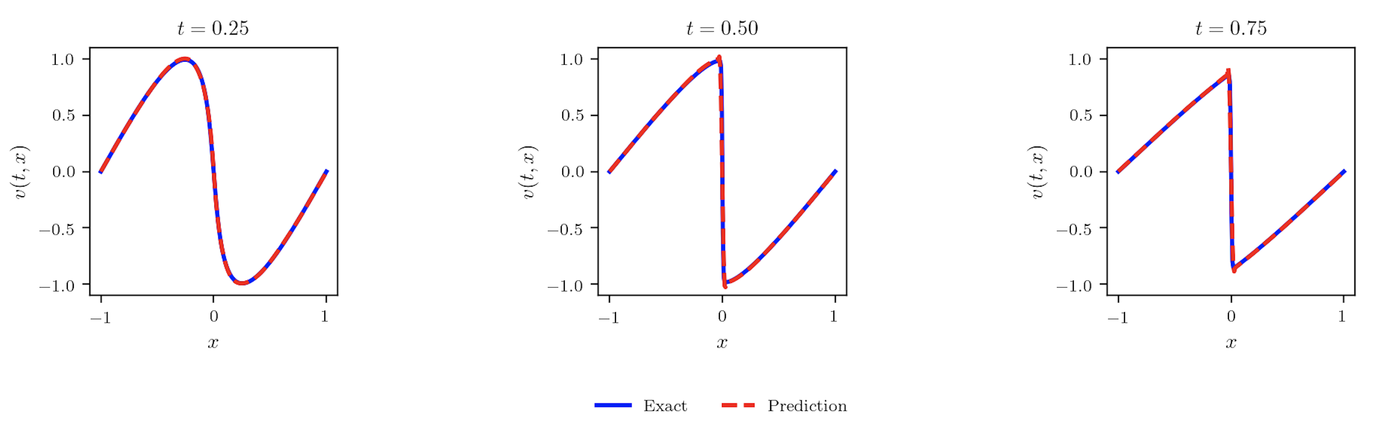
Figure 6: Example with $N_{d}=2000$ for the initial profile (A)

For the initial and periodic boundary condition (B), we generate $256\times 500=128000$ training data from the exact solution formula for the whole dynamics in time. With $N_{d}=2000$ training data, the PINN diverges frequently. We experiment with the model with 4000 or more data points to determine an appropriate number of training data. $L^{2}$-norm remains around $10^{-2}$ for all cases, which does not provide a clear cut. So, we use the absolute error of $\lambda_{1}$ to determine the appropriate number of training data. For each case of $N_{d}$, we perform the computation 5 to 10 times (Table 2).

$N_{d}$	$Error(\lambda_{1})$
4000	0.0207
6000	0.0113
8000	0.01059
10000	0.00965
12000	0.00908
14000	0.00848
16000	0.0046
18000	0.0059
20000	0.00604
25000	0.00671
30000	0.00611

Table 2: $Error(\lambda_{1})$ for various $N_{d}$ for the initial profile (B).

As $N_{d}$ increases, the results get better and need to do until it reaches the upper limit. Errors between 14000 and 18000 look better than other ranges. More than 18000 doesn’t seem to improve the results. $N_{d}=16000$ (12.5% of total data) is chosen. More than this doesn’t seem to be better. More likely almost the same. The average over ten computations is $\alpha\approx 0.0894$ with the relative error of $1.64\times 10^{-2}$.

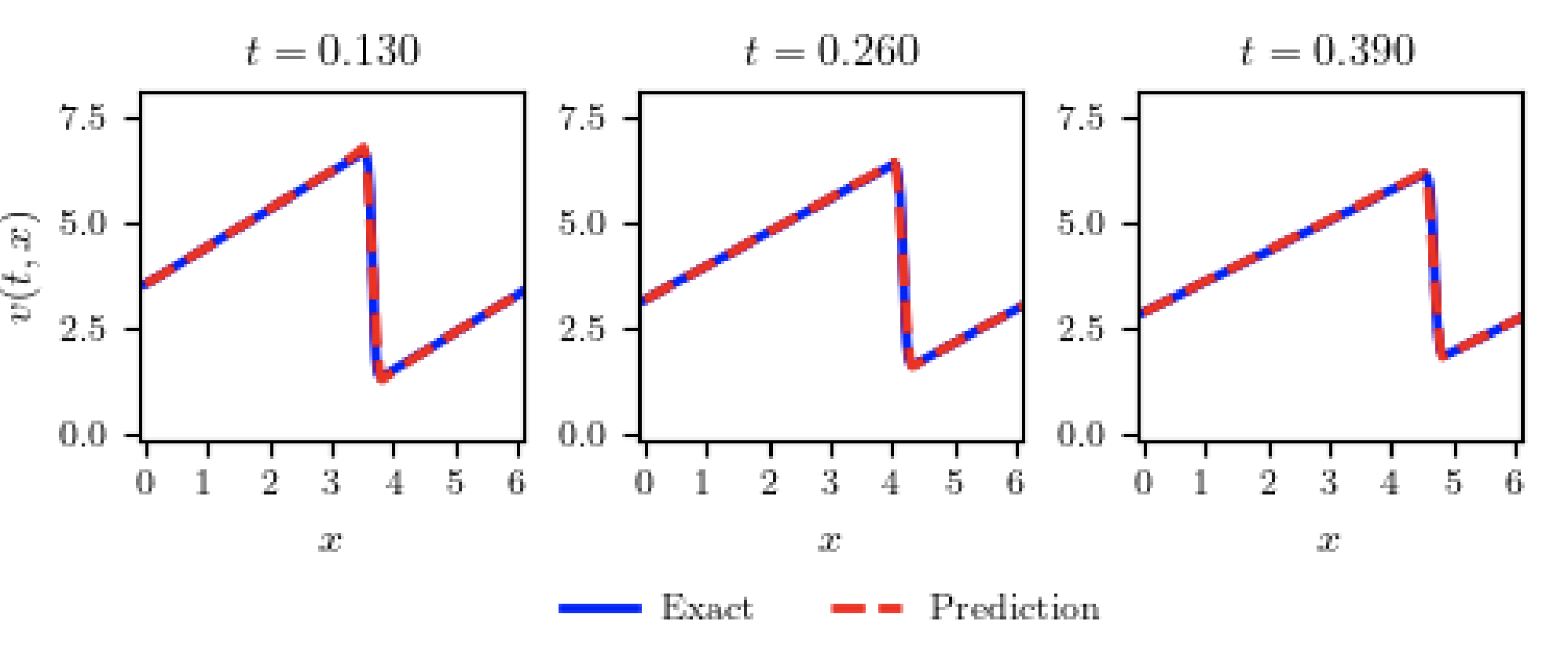
Figure 7: Example with $N_{d}=16000$ for the initial profile (B).

Every part of the solution for (B) moves to the right at the same speed, which differs from (A). In (A), the left side of a peak moves faster than the right side, developing a steeper middle. It resulted in a higher value of $\alpha$ with (B) than (A).

6 Experiment 3: The Filtered Vector $u$

We write the equation (1.1) in the filtered vector $u_{\alpha}=u$, which is a quasilinear evolution equation that consists of the inviscid Burgers equation plus $\mathcal{O}(\alpha^{2})$ nonlinear terms [2, 3, 4]:

$$u_{t}+uu_{x}=\alpha^{2}(u_{txx}+uu_{xxx}).$$ (6.1)

We compute the equation with the same conditions as in Section 4. The results show that the filtered equation (6.1) also tends to depend on the continuity of the initial profile as shown in Table 3.

IC	Continuous	IC	Discontinuous
I	0.0279	II	0.0004
III	0.0469	IV	0.0127
V	0.0469	VI	0.0277

Table 3: Averaged $\alpha$ values for the filtered vector $u$. with $N_{d}=2000$ and epochs $=10000$ except the case II. (IC = Initial Condition as in Section 4.)

When initial profiles contain discontinuities, the $\alpha$ values are much smaller than the ones with continuous initial profiles. Compared to the unfiltered equation (1.1), the $\alpha$ values for the filtered equation (6.1) are smaller, which may cause more oscillation in forward inferencing.

Also, with the initial profile (II), the parameter $\lambda_{1}$ for the filtered velocity is not close to 1 with $\epsilon(\lambda_{1})\approx 0.1076$ in average. By increasing the number of epochs from 10000 to 50000 we get a better result. $\lambda_{1}$ gets closer to 1 with $\epsilon(\lambda_{1})\approx 0.0531$, slightly better relative error and loss, which makes the solution become better at later time. Also, the oscillation near the discontinuity gets reduced. This verifies that $u$ needs very small $\alpha$ values to approximate the inviscid Burgers solution.

Figure 8: Examples with $N_{d}=2000$ for the initial profile (II). Top: epoch=10000.  Bottom: epoch=50000

7 Data-Driven Solutions of the Leray-Burgers Equation

In this section, we assess the validity of the $\alpha$-values by solving some initial-value problems with an MLP-PINN:

$$v_{t}+vv_{x}+\alpha^{2}v_{x}v_{xx}=0,\ x\in\mathbb{R},\ t\in(0,1)\ \ \mathrm{with\ the\ initial\ data,}\hskip 50.58878pt$$

$$\mathrm{(I)}\ \ v(0,x)=\left\{\begin{array}[]{cl}1&\mbox{if}\ x\leq 0\\ 1-x&\mbox{if}\ 0<x<1\\ 0&\mbox{if}\ x\geq 1\end{array}\right.\ \ \mathrm{or}\ \ \mathrm{(II)}\ \ v(0,x)=\left\{\begin{array}[]{cc}1&\mbox{if}\ x\leq 0\\ 0&\mbox{if}\ x>0.\end{array}\right.$$

To obtain the latent solution $\hat{v}_{\theta}^{*}$, we utilize an 8-hidden-layer MLP-based PINN with 20 neurons per layer and a hyperbolic tangent activation function. Our training set consists of a total of $N_{init}=10000$ data points randomly selected from $v(0,x)$. We also use $N_{r}=10000$ randomly sampled collocation points to enforce the Leray-Burgers equation within the solution domain. To optimize all loss functions, we employ the ADAM optimizer.

We compare PINN solutions with the exact analytic solutions of the inviscid Burgers equation obtained by the method of characteristics. Our computational focuses are as follows:

1. Convergence in $\alpha$. Whether the PINN solutions converge to those of the inviscid Burgers equation as $\alpha\rightarrow 0^{+}$.

2. Forward inference. Whether the PINN solutions capture the shock and rarefaction waves well and the trained $\alpha$-values are within the physically valid range.

3. Long-time extrapolation beyond training time. Whether the PINN can generate the solutions beyond training time.

7.1 The Convergence of the Leray-Burgers Solutions as $\alpha\rightarrow 0^{+}$

Figure 9 demonstrates that the Leray-Burgers equation effectively captures the shock formation with the continuous initial profile (I) within the range of $0<\alpha<0.05$. As $\alpha\rightarrow 0^{+}$, the Leray-Burgers solution converges to the inviscidt Burgers’ solution (the last graph in Figure 9).

With the discontinuous initial file (II), the Leray-Burgers equation still accurately captures the shock formation within the range of $0.01<\alpha<0.03$ (Figure 10). However, the MLP-based PINN generates spurious oscillations near the discontinuity at the beginning. Although the network quickly recovers and fits the oscillations as time progresses, the oscillations worsen, and non-linear instability arises as the $\alpha$ scale becomes smaller than 0.01. Consequently, the network solution deviates from the actual inviscid Burgers’ solution (the last graph in Figure 10). It indicates that a new neural network architecture is necessary to eliminate oscillations near discontinuities at the beginning of the computation.

Figure 11 shows the case of a rarefaction wave with initial discontinuity.

$$\mathrm{(IV)}\ \ v(0,x)=\left\{\begin{array}[]{cc}0&\mbox{if}\ x\leq 0\\ 1&\mbox{if}\ x>0.\end{array}\right.$$

As $\alpha\rightarrow 0^{+}$, the PINN solution converges to the inviscid Burgers solution. Interesting feature is that the spurious oscillation near the discontinuity reduces as $\alpha$ goes to 0, which is the opposite to the shock wave (II), Figure 10. We will compare the different behaviour of two cases in next section.

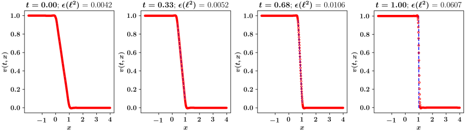
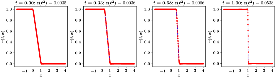
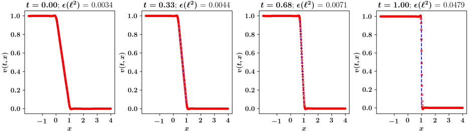
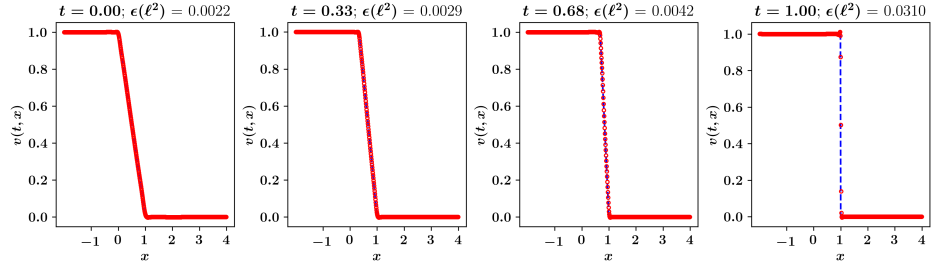
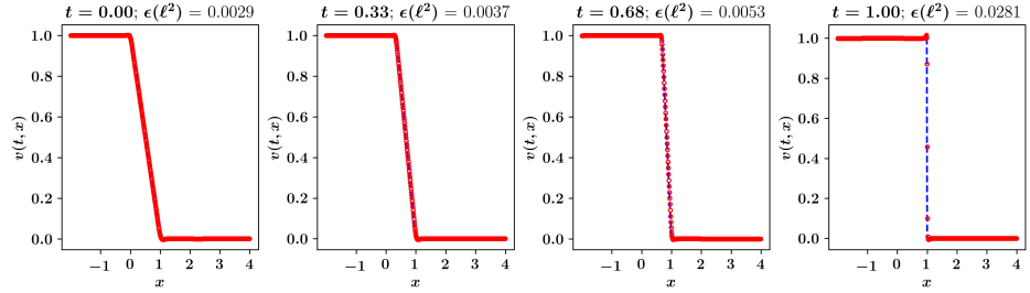
Figure 9: PINN solution with the initial profile (I) with $N_{init}=5000$, $N_{bdry}=5000$, and $N_{r}=10000$. $\alpha=0.05,0.04,0.03,0.01,0.0$ from the top with $\alpha=0$ (inviscid Burgers).

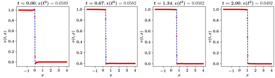
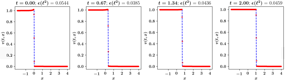
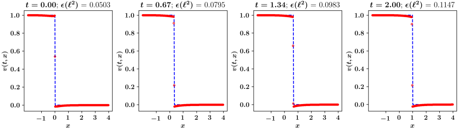
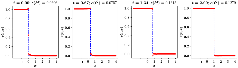
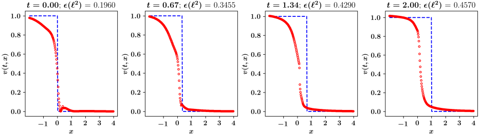
Figure 10: PINN solution with the initial profile (II) with $N_{init}=5000$, $N_{bdry}=5000$, and $N_{r}=10000$. $\alpha=0.03,0.025,0.015,0.01,0.0$ from the top with $\alpha=0$ (inviscid Burgers).

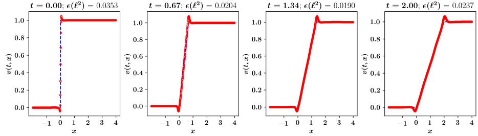
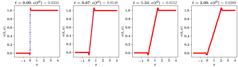
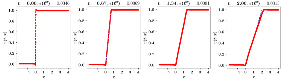
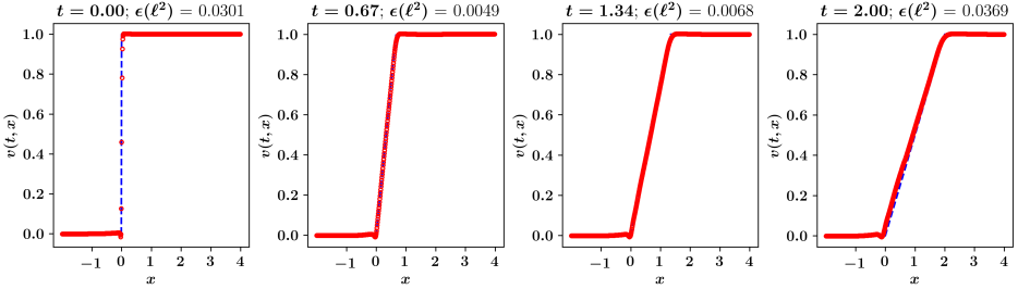
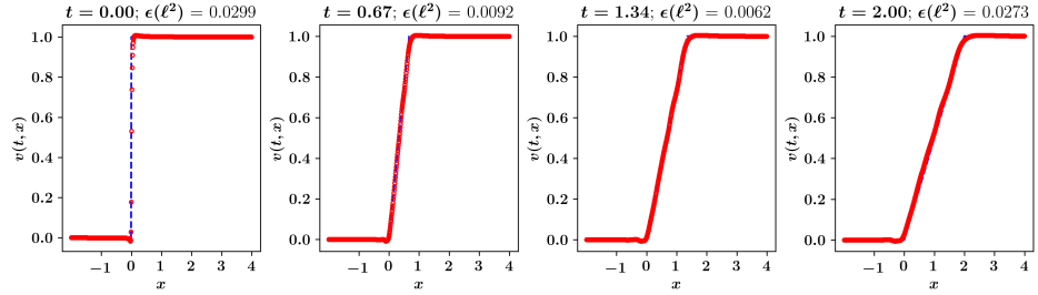
Figure 11: PINN solution with the initial profile (IV) with $N_{init}=5000$, $N_{bdry}=5000$, and $N_{r}=10000$. $\alpha=0.03,0.025,0.015,0.01,0.0$ from the top with $\alpha=0$ (inviscid Burgers).

7.2 The Evolution of the Relative Errors over Time

Figure 12 compares the relative errors of the Leray-Burgers solution with the initial profiles (II) and (IV), respectively. The upper picture, relative errors for profile (II) whose discontinuity travels over time, shows the evolution of relative errors of the shock wave solution over time, which reveals the PINN solution oscillates too much and diverges as $\alpha\rightarrow 0^{+}$. On the other hand, even though the initial profile contains a discontinuity, the PINN solution is not oscillatory for the rarefaction wave case (the bottom picture) and works smoothly, converging to the exact solution as $\alpha\rightarrow 0^{+}$.

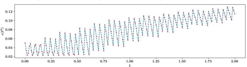
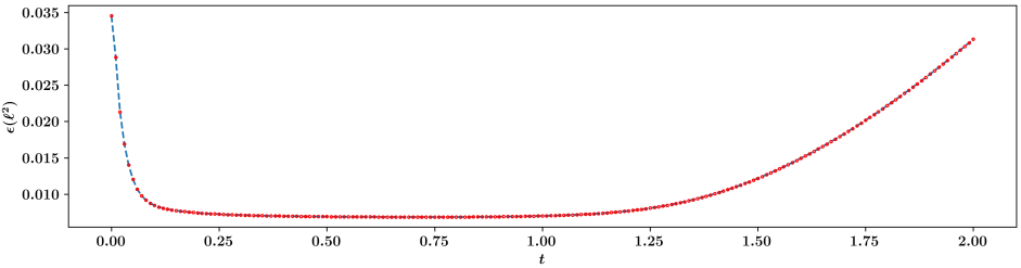
Figure 12: Relative errors over time for $\alpha=0.015$ with (II) (top) and (IV) (bottom).

This difference requires through analysis of the nature of the numerical solutions under the frame of neural networks to find the reasons for the oscillations that occur near discontinuities producing shock waves but not near the discontinuities generating rarefaction waves. New neural network architectures might be needed to remedy the issue of oscillations, preventing the convergence of the Leray-Burgers solutions as $\alpha$ goes to 0.

7.3 Forward Inference with Adaptively Optimized $\alpha>0$

In this section, we employ the Multilayer Perceptron (MLP)-based Physics-Informed Neural Network (PINN) to effectively learn the nonlinear operator $\mathcal{N}_{\alpha}[v]$, wherein $v$ represents the primary variable and $\alpha$ denotes a parameter. Coutinho, et all., [5], introduced the idea of adaptive artificial viscosity that can be learned during the training procedure and does not depend on an apriori choice of artificial viscosity coefficient. We incorporate the parameter $\alpha$ in place of artificial viscosity and make PINN train both $v$ and $\alpha$ to achieve a robust fit with the Leray-Burgers equation. Two examples highlight the Leray-Burgers equation’s capability of capturing a shock and a rarefaction waves as well as the corresponding optimal values of $\alpha$, which are presented in Figure 13.

The first graph showcases computational snapshots of the system’s evolution with the initial profile (II) over the time interval [0, 2]. It is important to note that the specific value of $\alpha$ depends on the randomness of the training data; however, it consistently remains around $\alpha\approx 0.027$. Throughout the temporal evolution, the relative error stays within the range of $10^{-2}$.

The second graph illustrates the snapshots of a rarefaction wave’s evolution with the initial profile (IV). Through the optimization process, an optimal $\alpha$ value is approximately $0.00627$, less than that of fixed $\alpha$ in Figure 10. Similar to the previous case, the relative error remains around $10^{-2}$ during the temporal evolution.

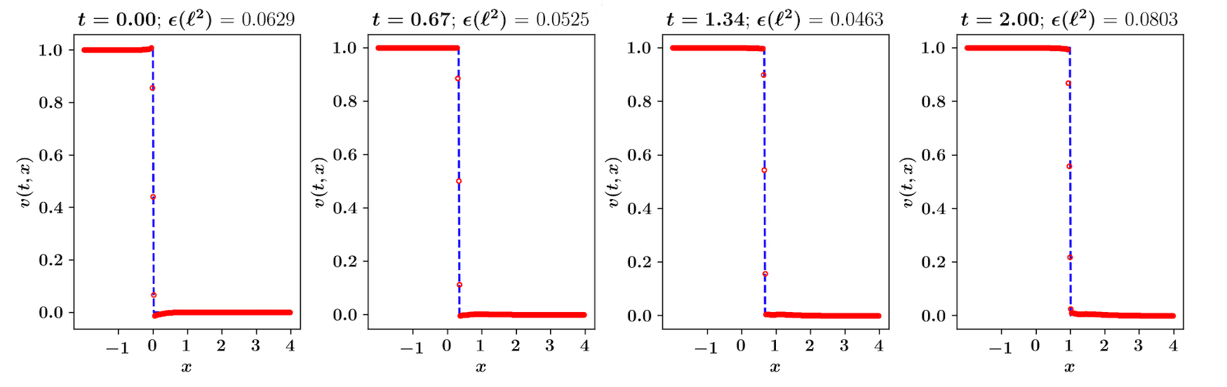
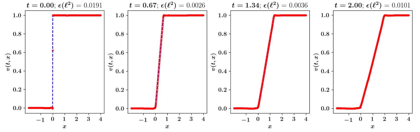
Figure 13: Optimal values: (II) $\alpha=0.02676$ (top) and (IV) $\alpha=0.00627$ (bottom).

7.4 Long-time extrapolation beyond training time

Here we address another key focus of our experiments revolving around the ability of the Physics-Informed Neural Network (PINN) to accurately predict solutions beyond the designated temporal domain for training. Specifically, we aim to assess the performance of PINN with respect to initial profiles (II) and (IV). The PINN was trained over a temporal interval spanning from 0 to 4, after which the computed solutions were extrapolated up to $t=12$. To evaluate the predictive capability of PINN in the extended time frame, we compared its solutions with the exact solutions obtained by the method of characteristics.

Figure 14 illustrates the discrepancy between the PINN solutions and the corresponding exact solutions beyond $t=4$. It becomes apparent from the figure that, as the temporal domain progresses beyond the training interval, the predictions generated by the PINN begin to deviate from the exact solutions. This is a PINN’s limitation and it is essential to address this shortcoming for the improvement of PINN algorithms.

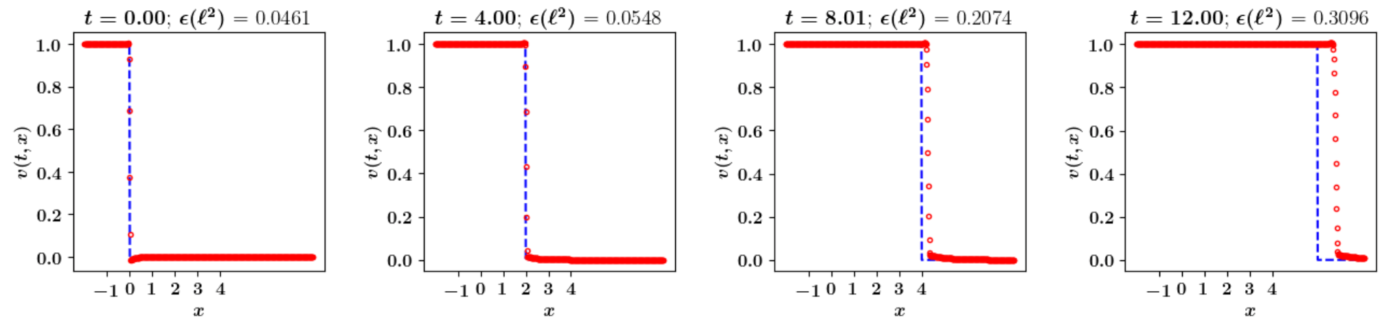
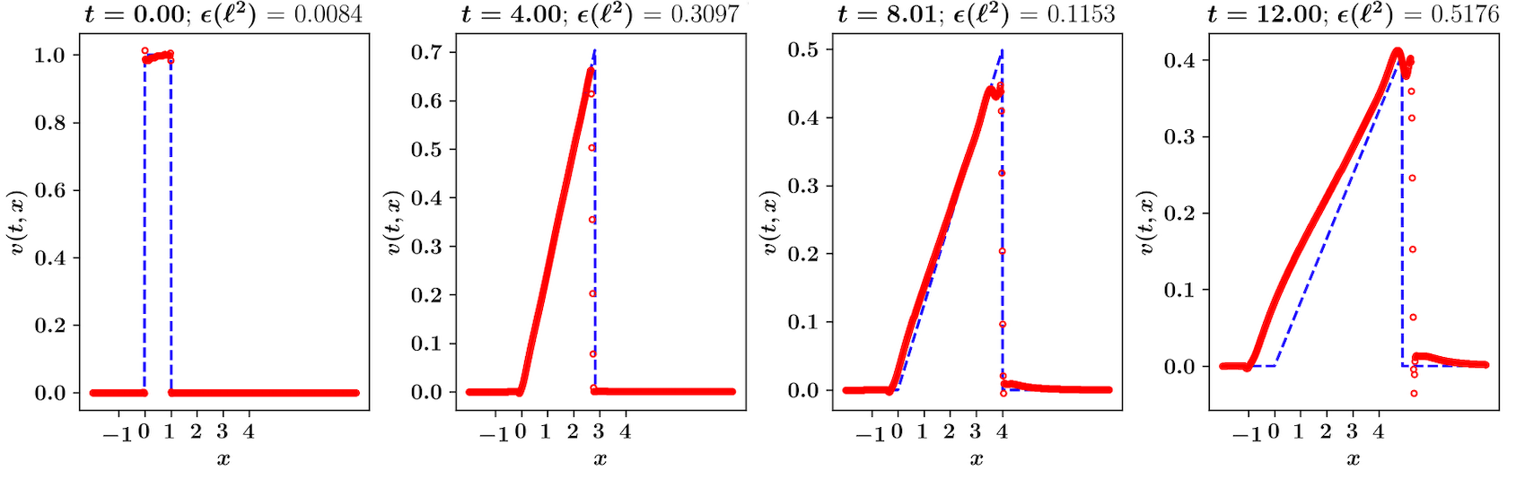
Figure 14: Training for $t\in[0,4]$: (II) $\alpha=0.027$ fixed (top) and (VI) $\alpha$ adaptively optimized (bottom).

8 Application to Traffic State Estimation

We apply the Leray-Burgers equation to a traffic state estimation to test its applicability to practical problems. Huang, et all., [10] applied PINNs to tackle the challenge of data sparsity and sensor noise in traffic state estimation (TSE). Main goal of TSE is to gain and provide a reliable description of traffic conditions in real-time. In Case Study-I in [10], they prepared the test-bed of a 5000-meter road segment for 300 seconds $\left((t,x)\in[0,300]\times[0,5000]\right)$. The spatial resolution of the dataset is 5 meters and temporal resolution is 1 second. The case study was designed to utilize the trajectory information data of Connected and Autonomous Vehicles (CAVs) as captured by Roadside Units (RSUs), which were deployed every 1000 meter on the road segment (6 RSUs on the 5000-meter road from $x=0$). The communication range of RSU was assumed to be 300 meters, meaning that vehicle information broadcast by CAVs at $x\in[0,300]$ can be captured by the first RSU and the second RSU can log CAV data transmitted at $x\in[700,1300]$, etc. More details on data acquisition and description can be found in [10, 11, 12].

In this section, we switch to the differential notation $\frac{d\rho}{dt},\frac{\partial\rho}{\partial x},\frac{\partial^{2}\rho}{\partial x^{2}}$ to avoid confusion with constant parameter notations such as $\rho_{m}$. Let $q(t,x)$ denote the flow rate indicating the number of vehicles that pass a set location in a unit of time and $\rho(t,x)$ the flow density representing the number of vehicles in a unit road of space. Then, the Lighthill-Whitham-Richards (LWR) traffic model [10] is, for $(t,x)\in\mathbb{R}^{+}\times\mathbb{R}$,

$$\frac{\partial\rho(t,x)}{\partial t}+\frac{\partial q(t,x)}{\partial x}=0,$$ (8.1)

where $\rho(t,x)=-\frac{\partial N(t,x)}{\partial x}$ and $q(t,x)=\frac{\partial N(t,x)}{\partial t}$. Here $N(t,x)$ is the cumulative flow of depicting the number of vehicles which have passed location $x$ by the time $t$. Huang, et all., [10] adopted the Greenshields fundamental diagram to set the relationship between traffic states - density $\rho$, flow $q$, and speed $v$:

$$q(\rho) =\rho v_{f}\left(1-\frac{\rho}{\rho_{m}}\right)$$ (8.2)

$$v(\rho) =v_{f}\left(1-\frac{\rho}{\rho_{m}}\right),$$ (8.3)

where $\rho_{m}$ is the jam density (maximum density) and $v_{f}$ is the free-flow speed. Substituting the relationship 8.2 into 8.1 transforms the LWR model into the LWR-Greenshield model

$$v_{f}\left(1-\frac{2\rho(t,x)}{\rho_{m}}\right)\frac{\partial\rho(t,x)}{\partial x}+\frac{\partial\rho(t,x)}{\partial t}=0.$$ (8.4)

We will just call it as the LWR model. The equation (8.4) is a hyperbolic PDE and a second order diffusive term can be added as following, to make the PDE become parabolic and secure a strong solution.

$$v_{f}\left(1-\frac{2\rho(t,x)}{\rho_{m}}\right)\frac{\partial\rho(t,x)}{\partial x}+\frac{\partial\rho(t,x)}{\partial t}=\epsilon\frac{\partial^{2}\rho}{\partial x^{2}}.$$ (8.5)

We will call the equation (8.5) as LWR-$\epsilon$ model. The second order diffusion term ensures the solution of PDE is continuous and differentiable, avoiding the breakdown and discontinuity in the solution. Following the same structural idea from (8.4) to (8.5) we add a regularization term to (8.4) instead of the diffusion term in (8.5):

$$v_{f}\left(1-\frac{2\rho(t,x)}{\rho_{m}}\right)\frac{\partial\rho(t,x)}{\partial x}+\frac{\partial\rho(t,x)}{\partial t}=-\alpha^{2}\frac{\partial\rho}{\partial x}\frac{\partial^{2}\rho}{\partial x^{2}}.$$ (8.6)

We will call the equation (8.6) as the LWR-$\alpha$ model. We set up the same PINN architecture for the computational comparisons of three models, LWR, LWR-$\epsilon$, and LWR-$\alpha$, with $v_{f}=25\,m/s,\rho_{m}=0.15\,vehicles/m$. Figure 15 visualizes the computational results.

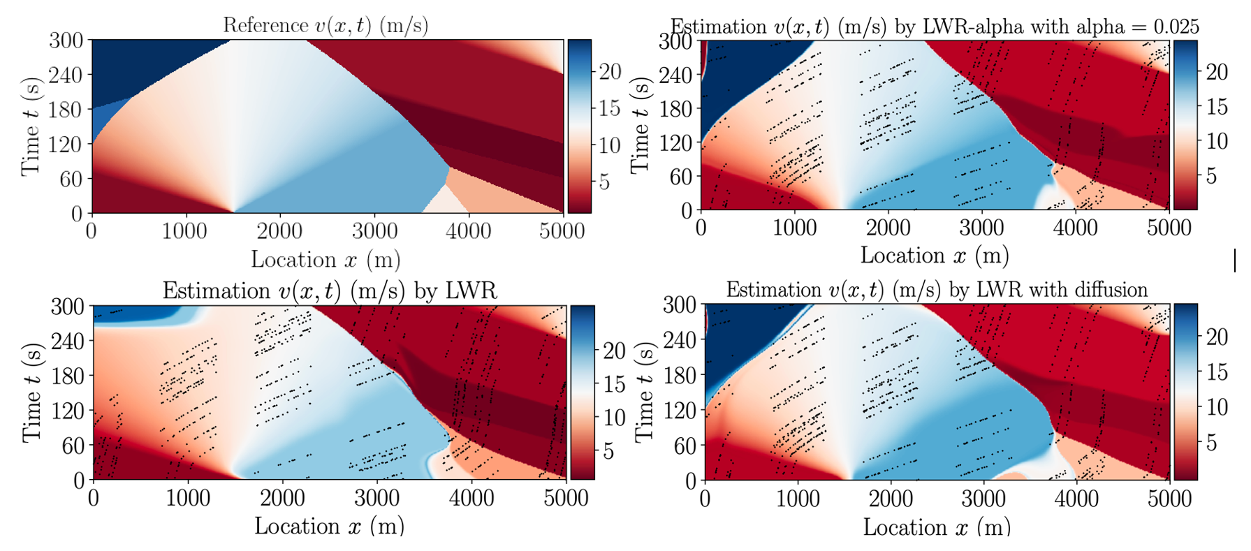
Figure 15: Traffic State Estimation: Reference Speed $v$, LWR-$\alpha$ Estimate ($\alpha=0.025$), LWR-$\epsilon$ ($\epsilon=0.025$), LWR Estimate, respectively counter-clockwise from the top left; Relative error $\approx 10^{-1}$; LWR-$\alpha$ training time is a little slower than LWR but much faster than LWR-$\epsilon$.

Our empirical calculations show that both the LWR-$\alpha$ and LWR-$\epsilon$ models give a reasonable approximation of the reference speed ($v$), as shown in Figure 15. Both models exhibit comparable accuracy to the standard LWR model, indicating their viability for traffic state estimation applications.

However, one notable distinction between the two variants is the computational time required for their simulations. The LWR-$\epsilon$ model exhibits significantly longer computational times, ranging from two to triple times that of the LWR-$\alpha$ and standard LWR models. This discrepancy arises from the fundamental difference between the LWR-$\alpha$ and LWR-$\epsilon$ models in their formulation. The LWR-$\alpha$ model modifies the convective term, resulting in a nonlinear behavior that better captures the inherent nonlinear characteristics of traffic data in space and time evolution. On the other hand, the LWR-$\epsilon$ model incorporates a linear viscous term, which lacks the same level of fidelity in representing the nonlinear traffic dynamics.

Our experiments underscore the significance of nonlinear characteristics in traffic data and their relevance for accurate traffic state estimation. The LWR-$\alpha$ model emerges as a more practical choice for traffic state estimation tasks due to its ability to account for the inherent nonlinear behavior in traffic flow. While the LWR-$\epsilon$ model may provide a reasonable approximation to the reference speed, its computational demand makes it less practical for real-time applications.

9 Conclusion

Computational experiments show that the $\alpha$-values depend on initial data. Specifically, the practical range of $\alpha$ spans from 0.01 to 0.05 for continuous initial profiles and narrows to 0.01 to 0.03 for discontinuous ones. We also note that the Leray-Burgers-$\alpha$ in terms of the filtered vector $u$ does not produce reliable estimates of $\alpha$. When approximating the filtered solution $u$ with commendable precision, the MLP-PINN necessitates a more extensive dataset, and the $\alpha$-value range for $u$ solutions appears confined, lying between 0.0001 and 0.005. Nonetheless, the MLP-PINN’s attempts with $u$ encounter challenges in converging to the true Burgers’ solutions. Thus, it is evident that the equation formulated in the unfiltered vector field $v$ offers a superior approximation to the exact Burgers equation.

In practical terms, treating $\alpha$ as an unknown variable becomes a prudent strategy. By endowing $\alpha$ with learnable attributes alongside network parameters, MLP-PINNs can be structured to unveil $\alpha$ within a valid range during the training process, potentially enhancing accuracy. Nevertheless, the MLP-PINN does generate spurious oscillations near discontinuities inherent in shock-inducing initial profiles. This phenomenon thwarts the PINN solution from aligning with an exact inviscid Burgers solution as $\alpha\rightarrow 0^{+}$. Furthermore, the MLP-PINN faces limitations in predicting solutions accurately beyond the prescribed temporal training domain. As the temporal domain progresses beyond the training interval, the predictions with the MLP-PINN begin to deviate from the exact solutions. To surmount these challenges, novel PINN algorithms are imperative to regulate oscillations and facilitate precise solution extrapolation beyond the designated temporal domain for training.

This study also demonstrates the effectiveness of the LWR-$\alpha$ model as a viable alternative for traffic state estimation. Surpassing the diffusion-based LWR-$\epsilon$ model in terms of computational efficiency, the LWR-$\alpha$ model aligns with the nonlinear nature of traffic data.

References

- [1] Raul K.C. Araújo1, Enrique Fernández-Cara and Diego A. Souza, On the uniform controllability for a family of non-viscous and viscous Burgers- systems, ESAIM: Control, Optimisation and Calculus of Variations, Volume 27, No. 78, (2021). (https://doi.org/10.1051/cocv/2021073)
- [2] Bhat, H. S., and Fetecau, R. C., A Hamiltonian Regularization of the Burgers Equation, Journal of Nonlinear Science, Vol. 16, (2006), pp. 615-638.
- [3] Bhat, H. S., and Fetecau, R. C., Stability of fronts for a regularization of the Burgers Equation, Quart. Appl. Math., Vol. 66, (2008), pp. 473–496.
- [4] Bhat, H. S., and Fetecau, R. C., The Rieman problem for the Leray-Burgers equation, Journal of Differential Equations, Vol. 246, (2009), pp. 3597–3979.
- [5] Emilio Jose Rocha Coutinho and Marcelo Dall’Aqua and Levi McClenny and Ming Zhong and Ulisses Braga-Neto and Eduardo Gildin, Physics-informed neural networks with adaptive localized artificial viscosity, Journal of Computational Physics, Vol. 489, (2023), pp. 112265. (https://doi.org/10.1016/j.jcp.2023.112265)
- [6] Georg A Gottwald, Dispersive regularizations and numerical discretizations for the inviscid Burgers equation, Journal of Physics A: Mathematical and Theoretical, Volume 40, Number 49, (November 2007).
- [7] Billel Guelmame, Stéphane Junca, Didier Clamond, Robert Pego, Global weak solutions of a Hamiltonian regularised Burgers equation, Journal of Dynamics and Differential Equations (2022). (https://doi.org/10.1007/s10884-022-10171-0)
- [8] Darryl D. Holm and Edriss S. Titi, Computational Models of Turbulence: The LANS- Model and the Role of Global Analysis, SIAM News, Vol. 38, No. 7, (2005).
- [9] Darryl D. Holm, Chris Jeffery, Susan Kurien, Daniel Livescu, Mark A. Taylor, and Beth A. Wingate, The LANS- Model for Computing Turbulence: Origins, Results, and Open Problems, Los Alamos Science, No. 19, (2005).
- [10] Archie J. Huang and Shaurya Agarwal, Physics-Informed Deep Learning for Traffic State Estimation: Illustrations With LWR and CTM models, IEEE Open Journal of Intelligent Transportation Systems, Vol. 3, (2022).
- [11] Archie J. Huang and Shaurya Agarwal, On the Limitations of Physics-Informed Deep Learning: Illustrations Using First-Order Hyperbolic Conservation Law-Based Traffic Flow Model, IEEE Open Journal of Intelligent Transportation Systems, Vol. 4, (2023).
- [12] Archie J. Huang and Shaurya Agarwal, Physics Informed Deep Learning: Applications in Transportation, arXiv:2302.12336 [cs.LG], (2023).
- [13] B. Kim and B. Nicolaenko, Existence and continuity of exponential attractors of the three dimensional Navier-Stokes- equations for uniformly rotating geophysical fluids, Communications in Mathematical Sciences, Vol. 4, No. 2, pages 399-452, (June 2006).
- [14] J. Leray, Essai sur le mouvement d’un fluide visqueux emplissant l’space, Acta Math. 63 (1934), 193–248.
- [15] Siddhartha Mishra and Roberto Molinaro, Estimates on the generalization error of physics-informed neural networks for approximating a class of inverse problems for PDEs, IMA Journal of Numerical Analysis (2022) 42, 981–1022.
- [16] Yekaterina S. Pavlova, Convergence of the Leray -Regularization Scheme for Discontinuous Entropy Solutions of the Inviscid Burgers Equation, The UCI Undergraduate Research Journal, (2006), 27-42.
- [17] Raissi, M., Perdikaris, P., and Karniadakis, G.E., Physics-informed neural networks: A deep learning framework for solving forward and inverse problems involving nonlinear partial differential equations, Journal of Computational Physics, Vol. 378, (2019), pp. 686–707.
- [18] Raissi, M., Perdikaris, P., and Karniadakis, G.E., Physics Informed Deep Learning (Part II): Data-driven Discovery of Nonlinear Partial Differential Equations, arXiv:1711.10566, (2017), pp. 1-19.
- [19] S.H. Rudy, S.L. Brunton, J.L. Proctor, J.N. Kutz, Data-driven discovery of partial differential equations, Science Advances, 3 (2017).
- [20] John Villavert and Kamran Mohseni, An Inviscid Regularization of Hyperbolic Conservation Laws, Journal of Applied Mathematics and Computing, 43, p55–73 (2013).
- [21] Sifan Wang, Parsi Perdikaris, Shyam Sankaran, Respecting Causality is All You Need for training Physics-Informed Neural Networks, (https://doi.org/10.48550/arXiv.2203.07404), (March 2022).
- [22] Ting Zhang and Chun Shen, Regularization of the Shock Wave Solution to the Riemann Problem for the Relativistic Burgers Equation, Abstract and Applied Analysis, Vol. (2014), Article ID 178672, 10 pages, (https://doi.org/10.1155/2014/178672).
- [23] Hongwu Zhao and Kamran Mohseni, A dynamic model for the Lagrangian-averaged Navier-Stokes- equations, Physics of Fluids, Vol. 17, 075106 (2005).