Two-parameter estimation with single squeezed-light interferometer via double homodyne detection

Abstract

The simultaneous two-parameter estimation problem in single squeezed-light Mach-Zehnder interferometer with double-port homodyne detection is investigated in this work. The analytical form of the two-parameter quantum Cramér-Bao bound defined by the quantum Fisher information matrix is presented, which shows the ultimate limit of the phase sensitivity will be further approved by the squeezed vacuum state. It can not only surpass the shot-noise limit, but also can even surpass the Heisenberg limit when half of the input intensity of the interferometer is provided by the coherent state and half by the squeezed light. For the double-port homodyne detection, the classical Fisher information matrix is also obtained. Our results show that although the classical Cramé-Rao bound does not saturate the quantum one, it can still asymptotically approach the quantum Cramér -Bao bound when the intensity of the coherent state is large enough. Our results also indicate that the squeezed vacuum state indeed can further improve the phase sensitivity. In addition, when half of the input intensity of the interferometer is provided by the coherent state and half by the squeezed light, the phase sensitivity obtained by the double-port homodyne detection can surpass the Heisenberg limit for a small range of the estimated phase.

1 Introduction

In quantum optical metrology, it aims to reach the ultimate sensitivity limit of the phase estimation imposed by quantum theory [1, 2]. Both Mach-Zehnder interferometer (MZI) and the SU(1,1) interferometer considered as the two-mode (two-path) interferometer have been used as a conventional device to realize precise measurement [3, 4]. In general, the phase sensitivity mainly depends on the probing quantum state of light. The ultimate precision bound of the phase sensitivity is given by the quantum Cramér-Rao bound (QCRB) for any possible measurement strategy [5]. For an MZI with classical probing states, the phase sensitivity of the estimated phase shift is bounded by the shot-noise limit (SNL) [3], $\Delta\phi=1/\sqrt{\bar{n}}$, where $\bar{n}$ is the mean photon number inside the interferometer. With the help of the nonclassical quantum states, such as squeezed states, entanglement states, it can beat the SNL, and even approach the Heisenberg limit (HL) [6, 7], $\Delta\phi=1/\bar{n}$ . In this case, the goal of the phase estimation is to reduce the QCRB until it surpasses the SNL, even approaches the HL. Up to the present, extensive theoretical and experimental research studies have been done for the single-parameter estimation via both optical interferometers with quantum resources [8, 9, 10, 11, 12, 13, 14, 15, 16, 17, 18, 19, 20, 21, 22, 23, 24]. Particularly, the squeezing resources is always a central strategy to improve the phase sensitivity and has thus become a crucial concept in quantum metrology. Recently, the quantum metrology advantage of the squeezing resources has been also demonstrated in experiments [23, 24].

In recent years, the multi-parameter estimation, i.e., the simultaneous estimation of several parameters, has received a lot of increasing interest [25, 26, 27, 28, 29, 30, 31, 32, 33, 34, 35, 36, 37, 38, 39, 40, 41]. It is often necessary to estimate multiple parameters simultaneously, such as biological system measurement [42, 43, 44] and quantum imaging [45, 46, 47]. However, the current frame work of multi-parameter estimation mainly has developed based on the quantum Fisher information matrix. As a consequence, the phase sensitivity is limited by the multi-parameter QCRB which is defined by the inverse of the quantum Fisher information matrix (QFIM). Few measurement schemes are proposed for studying the phase sensitivity of the multiparameter estimation. In 2014, the double-port homodyne detection has been shown as an optimal detection for the phase and the phase diffusion measurement for specific probe states [48]. Recently, two-parameter estimation with three-mode NOON state is investigated by the particle number measurement [49]. In this work, we will reexamine the original work by Yurke et al [4], and show that the signal of the homodyne detection in the MZI is not only depend on the phase difference $\phi_{d}=\phi_{1}-\phi_{2}$, but also on the phase sum $\phi_{s}=\phi_{1}+\phi_{2}$ for some input states. As a consequence, we propose a double-port homodyne detection to estimate simultaneously both $\phi_{1}$ and $\phi_{2}$ in a single squeezing-light MZI, and study its precision via the classical Fisher information matrix (CFIM).

It is known that the single-port homodyne detection may lose almost part of the phase information. Therefore, for single-parameter estimation, the double-port homodyne detection has been used to improve the phase sensitivity of the phase shift accumulated in the MZI [50, 51, 52, 53]. The results indicate that the better phase sensitivity can be obtained by the double-port homodyne detection [53]. In addition, for quantum illumination, a quantum receiver using the double-port homodyne detection shows better signal-to-noise ratio and is more robust against noise [54]. As mentioned above, it is well understood that the advantage of the squeezed resource in the single-parameter estimation. Here, we mainly investigate the quantum metrology advantage of the two-parameter estimation in a squeezing-light MZI with the $\phi_{1}-\phi_{2}$ model by the double-port homodyne detection.

The paper is organized as follows. In Sec. II, we reexamine the model and basic theory of the MZI with two unknown phase shifts in both arms, and show that the signal of the homodyne measurement is depend on both phases $\phi_{d}$ and $\phi_{s}$. In Sec. III, we consider a coherent state and a squeezed vacuum state (SVS) as the probing quantum state and investigate the QCRB of the each phase shift $\phi_{i}$ via the QFIM. Then, we investigate the performance of the double homodyne detection via the CFIM in Sec. IV. Our results show that the phase sensitivity of the estimated phase can asymptotically approach the QCRB. Finally, we summarize our results in Sec. V.

2 Model and basic theory

Let us consider a balanced MZI with the $\phi_{1}-\phi_{2}$ model which contains two 50:50 beam splitters and two phase shifts as illustrated in Fig. 1. The first beam splitter of this device is described by the unitary operator $\exp\left[-i\pi J_{1}/2\right]$, and the second beam splitter is represented by $\exp\left[i\pi J_{1}/2\right]$. The two estimated phase shifts $\phi_{1}$ and $\phi_{2}$ in the two arms of the MZI are described by a phase-shifting operator, $\hat{U}\left(\phi\right)=\exp\left[i\phi_{1}\hat{a}^{\dagger}\hat{a}+i\phi_{2}\hat{b}^{\dagger}\hat{b}\right]$. According to the SU(2) algebra of the angular momentum operators, the overall MZI transformation reads [4]

$$\hat{U}_{\text{MZI}}=e^{i\pi\hat{J}_{1}/2}e^{i\phi_{1}\hat{a}^{\dagger}\hat{a}+i\phi_{2}\hat{b}^{{\dagger}}\hat{b}}e^{-i\pi\hat{J}_{1}/2},$$ (1)

where these angular momentum operators can be written as

$$\hat{J}_{1} = \frac{1}{2}\left(\hat{a}^{\dagger}\hat{b}+\hat{a}\hat{b}^{\dagger}\right),J_{2}=\frac{1}{2i}\left(\hat{a}^{\dagger}\hat{b}-\hat{a}\hat{b}^{\dagger}\right),$$

$$\text{\ }\hat{J}_{3} = \frac{1}{2}\left(\hat{a}^{\dagger}\hat{a}-\hat{b}^{\dagger}\hat{b}\right),\hat{J}_{0}=\frac{1}{2}\left(\hat{a}^{\dagger}\hat{a}+\hat{b}^{\dagger}\hat{b}\right),$$ (2)

with the commutation relations $\left[\hat{J}_{i},\hat{J}_{j}\right]=i\epsilon_{ijk}\hat{J}_{k}$ ($i,j,k=1,2,3$). Here, $\hat{J}_{0}$ is a Casimir operator that commutes with all others, i.e., $\left[\hat{J}_{0},\hat{J}_{i}\right]=0$. And the operators $\hat{a}$ ($\hat{a}^{\dagger}$) and $\hat{b}$ ($\hat{b}^{\dagger}$) are the bosonic annihilation (creation) operators corresponding to two modes $a$ and $b$ of the interferometer, respectively. For our purpose, according to SU(2) algebra of the angular momentum operators and the Baker-Hausdorff lemma, Eq. (1) can be further recast as

$$\hat{U}_{\text{MZI}}=\exp\left(i\phi_{s}\hat{J}_{0}\right)\exp\left(i\phi_{d}\hat{J}_{2}\right),$$ (3)

where $\phi_{s}=\phi_{1}+\phi_{2}$ represents the phase sum and $\phi_{d}=\phi_{1}-\phi_{2\text{ }}$indicates the phase difference. Obviously, the MZI in its full generality is a two-parameter estimation problem since there are two unknown parameters, $\phi_{1}$ and $\phi_{2}$ (or $\phi_{d}$ and $\phi_{s}$), in the system.

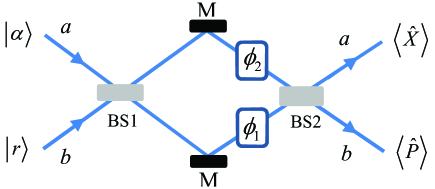
Figure 1: (Color online) Scheme of the double-output homodyne detection in a squeezed-state MZI with two-phase model.

As Yurke et al pointed [4], the operator $\exp\left[i\phi_{s}\hat{J}_{0}\right]$ contained the phase sum $\phi_{s}$ commutes with particle number operator. Therefore, in the view of the measurement, it does not contribute to the expectation values of the number-conserving operators. For example, for a photon-number-resolving detection, it is described by the projection operator $\left|m,n\right\rangle\left\langle m,n\right|$ where $\left|m,n\right\rangle=\hat{a}^{\dagger m}\hat{b}^{\dagger}\left|0,0\right\rangle/\sqrt{m!n!}$ is the two-mode Fock state. When an arbitrary input $\hat{\rho}_{\text{in}}$ propagates through the MZI, the resulted output state $\hat{\rho}_{\text{out}}$ evolves to

$$\hat{\rho}_{\text{out}}=\hat{U}_{\text{MZI}}\hat{\rho}_{\text{in}}\hat{U}_{\text{MZI}}^{{\dagger}}.$$ (4)

Then, according to Eq. (4), in the Heisenberg picture, the corresponding signal Tr$\left(\hat{\rho}_{\text{out}}\left|m,n\right\rangle\left\langle m,n\right|\right)$ of the photon-number-resolving detection reads

$$\text{Tr}\left\{\hat{\rho}_{\text{in}}\exp\left(-i\phi_{d}\hat{J}_{y}\right)\left|m,n\right\rangle\left\langle m,n\right|\exp\left(i\phi_{d}\hat{J}_{y}\right)\right\}.$$ (5)

Obviously, the operator $\exp\left(i\phi_{s}\hat{J}_{0}\right)$ contained the phase sum factor does not contribute to the expectation values of the photon-number-resolving detection for an arbitrary input state. In deriving Eq. (5), the following the transformations $\exp\left(-i\phi_{s}\hat{J}_{0}\right)\hat{a}^{\dagger}\exp\left(i\phi_{s}\hat{J}_{0}\right)=\hat{a}^{\dagger}\exp\left(-i\phi_{s}/2\right)$ and $\exp\left(-i\phi_{s}\hat{J}_{0}\right)\hat{b}^{{\dagger}}\exp\left(i\phi_{s}\hat{J}_{0}\right)=\hat{b}^{{\dagger}}\exp\left(-i\phi_{s}/2\right)$ have been used. It can be seen that, for intensity detection or parity detection based on the photon-number-resolving detector, including the photon-number-resolving detection, the signals of these measurements are only depended on the phase difference $\phi_{d}$. As a consequence, in the past decades, one is usually interested in the phase difference contained in the MZI. Especially, one main consider two phase-shift configurations: one is the phase anti-symmetrically distribution, i.e., $\phi_{1}=-\phi/2$ and $\phi_{2}=\phi/2$, another is the phase shift only occurs in one mode of the interferometer (for example $\phi_{1}=\phi$ and $\phi_{2}=0$).

However, according to the characteristics of the structure of the MZI expressed by Eq. (3), the signal of the homodyne detection is usually sensitive to both $\phi_{d}$ and $\phi_{s}$ for some input states. Therefore, we need consider both QFIM and CFIM to investigate the phase sensitivity. In the following, we will investigate the two-parameter estimation in a single MZI with the $\phi_{1}-\phi_{2}$ model via the double-port homodyne detection.

3 The QCRB of two-parameter estimation

In the multi-parameter estimation, we need introduce the multi-parameter QCRB, which is inversely proportional to the quantum Fisher information, i.e., the bound is given by

$$\sum_{i}\left(\Delta^{2}\phi_{i}\right)_{\text{QCRB}}=\text{Tr}\left[\left(F^{q}\right)^{-1}\right],$$ (6)

where $\sum_{i}\left(\Delta^{2}\phi_{i}\right)_{\text{QCRB}}$ is the total variance for multi-parameter estimation to quantity the measurement precision, and $\left(F^{q}\right)^{-1}$ is the inverse of the QFIM. In the MZI with the $\phi_{1}-\phi_{2}$ model, the matrix elements $F_{ij}^{q}$ of the two-by-two QFIM is defined as

$$F_{ij}^{q}=4\mathrm{Re}\left[\left\langle\partial_{i}\psi\left(\phi\right)\right|\left|\partial_{j}\psi\left(\phi\right)\right\rangle-\left\langle\partial_{i}\psi\left(\phi\right)\right|\left|\psi\left(\phi\right)\right\rangle\left\langle\psi\left(\phi\right)\right|\left|\partial_{j}\psi\left(\phi\right)\right\rangle\right],$$ (7)

with $\left|\psi\left(\phi\right)\right\rangle=\hat{U}\left(\phi\right)\exp\left[-i\pi J_{x}/2\right]\left|\text{in}\right\rangle$ is the probing state after sensing both phase shifts and $\left|\partial_{i}\psi\left(\phi\right)\right\rangle=\partial\left|\psi\left(\phi\right)\right\rangle/\partial\phi_{i}$. The subscript ”$i$” and ”$j$” denote the $1$ and $2$, respectively. It can be seen that the QFIM is solely determined by the parameterized output state and its dependence on the parameters. In addition, it is well known that the QCRB defined by the QFIM gives an ultimate bound of the phase sensitivity over all possible measurements.

Here, we consider a coherent state and an SVS, $\left|\text{in}\right\rangle=\left|z\right\rangle_{a}\left|r\right\rangle_{b}$, as the probing state of the MZI. The SVS is defined by $\left|r\right\rangle=\mathrm{sech}^{1/2}r\exp\left[-\hat{b}^{\dagger 2}\tanh re^{i\theta_{s}}/2\right]\left|0\right\rangle$. The average total photon number of the input state is given by $\bar{n}_{\text{in}}=\left|z\right|^{2}+\sinh^{2}r$. For the convenience, we rewrite the SVS in the basis of the coherent state

$$\left|r\right\rangle=\mathrm{sech}^{1/2}r\int\frac{d^{2}\beta}{\pi}e^{-\frac{1}{2}\left|\beta\right|^{2}-\frac{\tanh r}{2}e^{i\theta_{s}}\beta^{\ast 2}}\left|\beta\right\rangle,$$ (8)

where $\left|\beta\right\rangle$ represents a coherent state. Then, we can further obtain the expectation of the operator $\hat{b}^{{\dagger}n}\hat{b}^{m}$ in the SVS

$$\left\langle r\right|\hat{b}^{{\dagger}n}\hat{b}^{m}\left|r\right\rangle=\frac{\partial^{m+n}}{\partial t^{m}\partial\tau^{n}}\exp\left[-\left(t^{2}e^{-i\theta_{s}}+\tau^{2}e^{i\theta_{s}}\right)\frac{\sinh 2r}{4}+\tau t\sinh^{2}r\right]_{t,\tau=0}.$$ (9)

Given the probe state, we can now calculate the matrix elements of the QFIM. According to Eqs. (7) and 9, we obtain the corresponding QFIM, i.e.,

$$F^{q}=\left[\begin{array}[]{cc}F_{11}^{q}&F_{12}^{q}\\ F_{21}^{q}&F_{22}^{q}\end{array}\right],$$ (10)

with the matrix elements

$$F_{11}^{q}=F_{22}^{q}=\left(2\sinh^{2}r+3\right)\sinh^{2}r+\left|z\right|^{2}\left(1+e^{2r}\right),$$ (11)

and

$$F_{12}^{q}=F_{21}^{q}=\left(2\sinh^{2}r+1\right)\sinh^{2}r+\left|z\right|^{2}\left(1-e^{2r}\right).$$ (12)

In order to maximize the QCRB, we have adopted the combined phase $2\psi+\theta_{s}=2k\pi$ ($k=0,1,2\cdots$). The factor $\psi$ is the phase of the complex amplitude $z$ of the coherent state $\left|z\right\rangle$. In the MZI with the $\phi_{1}-\phi_{2}$ model, we mainly focus on the estimation of each phase shift $\phi_{i}$. For $\phi_{1}$ or $\phi_{2}$, it can be seen from Eqs. (10-12) that the QCRB is the same, i.e., the ultimate bound of the phase sensitivity of the phase shift $\phi_{1}$ or $\phi_{2}$ reads

$$\left(\Delta^{2}\phi_{i}\right)_{\text{QCRB}} = \frac{F_{ii}^{q}}{\left(F_{ii}^{q}\right)^{2}-\left(F_{i,j}^{q}\right)^{2}}$$ (13)

$$= \frac{\left(2\sinh^{2}r+3\right)\sinh^{2}r+\left|z\right|^{2}\left(1+e^{2r}\right)}{2\left(\sinh^{2}r+\left|z\right|^{2}e^{2r}\right)\left(\sinh^{2}2r+2\left|z\right|^{2}\right)}.$$

These results expressed by Eqs. (10-12) are somewhat different from that results expressed by Eq. (10) in Ref. [55]. This is because that here we calculate the QFIM in basis $\phi_{1}$ and $\phi_{2}$, i.e., the MZI with the $\phi_{1}-\phi_{2}$ model. While, QFIM is obtained in basis $\phi_{d}$ and $\phi_{s}$ in Ref. [55]. Particularly, in the case of $r=0$, Eq. (13) reduces to $\left(\Delta^{2}\phi_{i}\right)_{\text{QCRB}}|_{r=0}=1/\left(2\left|z\right|^{2}\right)$. Actually, for the MZI with the $\phi_{1}-\phi_{2}$ model, the QCRB of each phase shift $\phi_{i}$ can still surpass the SNL, even one mode of the interferometer is a vacuum state as shown in Eq. (13). It is interesting that, in the case of the $\left|z\right|^{2}=\sinh^{2}r=\bar{n}_{\text{in}}/2$, Eq. (13) reduces to

$$\left(\Delta^{2}\phi_{i}\right)_{\text{QCRB}}=\frac{\left(3+\bar{n}_{\text{in}}\right)+\left(2+\bar{n}_{\text{in}}+\sqrt{\bar{n}_{\text{in}}\left(2+\bar{n}_{\text{in}}\right)}\right)}{2\bar{n}_{\text{in}}\left(2+\bar{n}_{\text{in}}+\sqrt{\bar{n}_{\text{in}}\left(2+\bar{n}_{\text{in}}\right)}\right)\left(3+\bar{n}_{\text{in}}\right)}.$$ (14)

which can surpass the HL. At the same time, the QCRB reaches its minimum in the case of $\left|z\right|^{2}=\sinh^{2}r$ for a give mean photon number of the input state. On the other hand, according to Eq. (11) when the phase shift is generated only in one mode of the MZI, the QCRB can described by $1/F_{ii}^{q}$, i.e.,

$$\left(\Delta^{2}\phi\right)_{\text{QCRB}}=\frac{1}{\left(2\sinh^{2}r+3\right)\sinh^{2}r+\left|z\right|^{2}\left(1+e^{2r}\right)},$$ (15)

which is consistent with the Eq. (4) in Ref.[55].

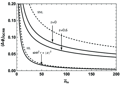
Figure 2: (Color online) The QCRB of the phase $\phi_{i}$ as a function of the total mean photon number inside the interferometer for given $r=0.0$ and $r=0.6$. The upper black dashed line denotes the SNL, while the below black dashed line represents the HL.

In order to illustrate the Eq. (13) explicitly and more exactly, we plot the QCRB with respect to the average total photon number $\bar{n}_{\text{in}}$ in Fig. 2. It can be seen that the SVS can further improve the QCRB. In addition, in the case of the $\left|z\right|^{2}=\sinh^{2}r=\bar{n}_{\text{in}}/2$, the QCRB can even surpass the HL. It may be an interesting result. It should be noted that, for the single-parameter estimation, very recently it has been shown in experiment that the phase sensitivity obtained by the double-port homodyne detection with an SVS as a probe can surpass the HL as well as the ideal N00N state protocol [23].

4 Two-parameter estimation with single squeezed-light MZI via double-port homodyne detection

As mentioned above, for the MZI with two estimated phase shifts, the signal of the the parity detection, intensity detection and photon-number-resolving detection is only sensitive to the phase difference. However, for the homodyne detection, things are somewhat different. Here, we first demonstrate analytically that the signal of the homodyne detection is sensitive to both $\phi_{d}$ and $\phi_{s}$ for a coherent state and an SVS considered as the probe state. Then, we consider the simultaneous estimation of the two phase shifts $\phi_{1}$ and $\phi_{2}$ in a squeezing-light MZI via double-port homodyne detection, and study its precision based on the CFIM.

4.1 The signal of the double-port homodyne detection

The homodyne detection is modeled as projection on quadratures of the bosonic filed described by the standard quadrature operator [56], i.e.,

$$\hat{X}\left(\theta\right)=\frac{\hat{a}e^{-i\theta}+\hat{a}^{\dagger}e^{i\theta}}{\sqrt{2}},$$ (16)

where $\theta$ is a phase of the strong local oscillator. Here, we consider the double-port homodyne detection as shown in Fig. 1. The two outports of the interferometer are projected on the $\hat{X}_{a}=\hat{X}\left(0\right)$ and $\hat{P}_{b}=\hat{X}\left(\pi/2\right)$ quadratures via the homodyne measurement. Here, the subscripts ”$a$” and ”$b$” denote two different field modes $a$ and $b$ of the interferometer. According to Eq. (4), for an arbitrary input state $\hat{\rho}_{\text{in}}$, the signal of the homodyne detection in the Heisenberg picture reads

$$\left\langle\hat{X}\left(\theta\right)\right\rangle=\text{Tr}\left\{\hat{\rho}_{\text{in}}\hat{U}_{\text{MZI}}^{\dagger}\hat{X}\left(\theta\right)\hat{U}_{\text{MZI}}\right\}.$$ (17)

Then, noting that the following field operator transformations of the MZI

$$\hat{U}_{\text{MZI}}^{\dagger}\hat{a}\hat{U}_{\text{MZI}} = \left(\hat{a}\cos\frac{\phi_{d}}{2}+\hat{b}\sin\frac{\phi_{d}}{2}\right)\exp\left(i\frac{\phi_{s}}{2}\right),$$

$$\hat{U}_{\text{MZI}}^{\dagger}\hat{b}\hat{U}_{\text{MZI}} = \left(-\hat{a}\sin\frac{\phi_{d}}{2}+\hat{b}\cos\frac{\phi_{d}}{2}\right)\exp\left(i\frac{\phi_{s}}{2}\right),$$ (18)

one can clearly see that the signal of the homodyne detection, in general, depends on both $\phi_{d}$ and $\phi_{s}$ for the input state $\hat{\rho}_{\text{in}}$. Enlighten by this result, in the following we will investigate the two-parameter estimation with a squeezing-light MZI via the double-port homodyne detection. When we consider a coherent state and an SVS, $\hat{\rho}_{\text{in}}=\left|z\right\rangle_{a}\left|r\right\rangle_{b}\left.{}_{b}\left\langle r\right|_{a}\left\langle z\right|\right.$, as the probing state of the MZI, according to Eq. (17), we can immediately obtain the signals of the double-port homodyne detection, i.e.,

$$\left\langle\hat{X}_{a}\right\rangle=\sqrt{2}\left|z\right|\cos\frac{\phi_{d}}{2}\cos\left(\psi+\frac{\phi_{s}}{2}\right),$$ (19)

and

$$\left\langle\hat{P}_{b}\right\rangle=-\sqrt{2}\left|z\right|\sin\frac{\phi_{d}}{2}\sin\left(\psi+\frac{\phi_{s}}{2}\right),$$ (20)

respectively. One can clearly see that the signal of the homodyne detection depends on both the phase difference and phase sum for an such probe state. As a consequence, one can simultaneously obtain the values of both phases $\phi_{1}$ and $\phi_{2}$ via Eqs. (19) and (20). In addition, the different phase-configuration will lead to the different signals of the measurement, even for single-parameter estimation. For example, if we are only interested in the single phase difference $\phi_{d}$, we still will obtain different values of the quantum Fisher information when we choice different phase-configurations [57, 58], e.g., the phase-configuration with $\phi_{1}=-\phi/2$ and $\phi_{2}=\phi/2,$ or the case of $\phi_{1}=\phi$ and $\phi_{2}=0$ (or $\phi_{1}=0,\phi_{2}=\phi$ ). This result is also occurred in the phase estimation of the SU(1,1) interferometer [59, 60]. Therefore, this two-parameter model of the MZI, as shown in Eq. (3), explicitly shows that one does not know the phase $\phi_{s}$ in prior. This will affect the precision limit of the phase sum $\phi_{d}$ especially when $\phi_{d}$ and $\phi_{s}$ are correlated. As a consequence, we need calculate the two-by-two CFIM with respect to the double homodyne detection ($\hat{X}$, $\hat{P}$) to access the measurement precision.

4.2 Sensitivity determined by the classical Fisher information matrix

The Fisher information lies at the heart of the phase sensitivity of the estimated phases. In quantum metrology, the CRB is determined by the CFIM and sets the ultimate limit bound of the phase sensitivity with a specific measurement strategy. For the MZI with the $\phi_{1}-\phi_{2}$ model, its CFIM is given by a two-by-two matrix [61]

$$F^{c}=\left[\begin{array}[]{cc}F_{11}^{c}&F_{12}^{c}\\ F_{21}^{c}&F_{22}^{c}\end{array}\right],$$ (21)

where the subscript $1$ and $2$ correspond to $\phi_{1}$ and $\phi_{2}$. After a sequence of detection events, one can obtain the two-parameter CRB to quantify the phase sensitivity, i.e.,

$$\sum_{i}\left(\Delta^{2}\phi_{i}\right)=\text{Tr}\left[\left(F^{c}\right)^{-1}\right],$$ (22)

Therefore, the CRB of the two-parameter estimation with a given measurement is determined by the Tr$\left[\left(F^{c}\right)^{-1}\right]$. Because the results ($x_{a},p_{b}$) of the measurement ($\hat{X}_{a}$, $\hat{P}_{b}$) are continuous variables, the elements of the CFIM should be expressed in the integral form

$$F_{i,j}^{c}=\int\frac{dx_{a}dp_{b}}{p\left(x_{a},p_{b}|\phi_{1},\phi_{2}\right)}\frac{\partial p\left(x_{a},p_{b}|\phi_{1},\phi_{2}\right)}{\partial\phi_{i}}\frac{\partial p\left(x_{a},p_{b}|\phi_{1},\phi_{2}\right)}{\partial\phi_{j}}$$ (23)

where the subscript ”$i$” and ”$j$” denote $1$ and $2$, and $p\left(x_{a},p_{b}|\phi_{1},\phi_{2}\right)$ is the phase-dependent probability distribution of the measurement results ($x_{a},p_{b}$). For the double-homodyne detection, the conditional probability function $p\left(x_{a},p_{b}|\phi_{1},\phi_{2}\right)$ is just the expectation value of the projection operator $\left|x_{a},p_{b}\right\rangle\left\langle x_{a},p_{b}\right|$ in the output state, i.e.,

$$p\left(x_{a},p_{b}\right)|\left(\phi_{s},\phi_{d}\right)=\text{Tr}\left[\hat{U}_{\text{MZI}}\hat{\rho}_{\text{in}}\hat{U}_{\text{MZI}}^{{\dagger}}\left|x_{a},p_{b}\right\rangle\left\langle x_{a},p_{b}\right|\right],$$ (24)

where the coordinate and momentum eigenstate $\left|x_{a},p_{b}\right\rangle$ reads [62]

$$\left|x_{a},p_{b}\right\rangle = \left(\frac{1}{\pi}\right)^{1/2}\exp\left[-\frac{x_{a}^{2}}{2}+\sqrt{2}x_{a}\hat{a}^{{\dagger}}-\frac{\hat{a}^{{\dagger}2}}{2}\right]\left|0\right\rangle_{a}$$ (25)

$$\otimes\exp\left[-\frac{p_{b}^{2}}{2}+i\sqrt{2}p_{b}\hat{b}^{{\dagger}}+\frac{\hat{b}^{{\dagger}2}}{2}\right]\left|0\right\rangle_{b}.$$

For the input state $\hat{\rho}_{\text{in}}=\left|z\right\rangle_{a}\left|r\right\rangle_{b}\left.{}_{b}\left\langle r\right|_{a}\left\langle z\right|\right.$, according to Eq. (24), after long but straightforward calculation, we can obtain the probability of the outcome ($x_{a},p_{b}$)

$$P\left(x_{a},p_{b}\right)|\left(\phi_{1},\phi_{2}\right) = \frac{A_{0}}{\pi}\exp\left[A_{1}x_{a}+B_{1}p_{b}\right.$$ (26)

$$\left.-A_{2}x_{a}^{2}-B_{2}p_{b}^{2}+C_{0}x_{a}p_{b}+D_{0}\right],$$

where

$$A_{0} = \left[\cosh^{2}r+\cos\phi_{d}\cos\left(\phi_{s}+\theta_{s}\right)\sinh 2r+\cos^{2}\phi_{d}\sinh^{2}r\right]^{-1/2},$$

$$C_{0} = -A_{0}^{2}\sin\phi_{d}\sin\left(\phi_{s}+\theta_{s}\right)\sinh 2r,$$

$$D_{0} = -\left|z\right|^{2}\left[\cos\phi_{d}\cos\left(\phi_{s}+2\psi\right)\left(1+A_{0}^{2}\sin^{2}\phi_{d}\sinh^{2}r\right)\right.$$ (27)

$$\left.+A_{0}^{2}\sin^{2}\phi_{d}\cos\left(2\phi_{s}+\theta_{s}+2\psi\right)\sinh r\cosh r\right],$$

and

$$A_{1} = 2\sqrt{2}\left|z\right|\left[\cos\frac{\phi_{d}}{2}\cos\left(\frac{\phi_{s}}{2}+\psi\right)\right.$$

$$\left.+\frac{1}{2}A_{0}^{2}\sin\frac{\phi_{d}}{2}\sin 2\phi_{d}\cos\left(\frac{\phi_{s}}{2}+\psi\right)\sinh^{2}r\right.$$

$$\left.+A_{0}^{2}\sin\frac{\phi_{d}}{2}\sin\phi_{d}\cos\left(\frac{3}{2}\phi_{s}+\theta_{s}+\psi\right)\sinh r\cosh r\right],$$

$$B_{1} = 2\sqrt{2}\left|z\right|\left[-\sin\frac{\phi_{d}}{2}\sin\left(\frac{\phi_{s}}{2}+\psi\right)\right.$$ (28)

$$\left.+\frac{1}{2}A_{0}^{2}\cos\frac{\phi_{d}}{2}\sin 2\phi_{d}\sin\left(\frac{\phi_{s}}{2}+\psi\right)\sinh^{2}r\right.$$

$$\left.+A_{0}^{2}\cos\frac{\phi_{d}}{2}\sin\phi_{d}\sin\left(\frac{3}{2}\phi_{s}+\theta_{s}+\psi\right)\sinh r\cosh r\right],$$

as well as

$$A_{2} = 1+2A_{0}^{2}\sin^{2}\frac{\phi_{d}}{2}\cos\phi_{d}\sinh^{2}r$$

$$+2A_{0}^{2}\sin^{2}\frac{\phi_{d}}{2}\cos\left(\phi_{s}+\theta_{s}\right)\sinh r\cosh r,$$

$$B_{2} = 1-2A_{0}^{2}\cos^{2}\frac{\phi_{d}}{2}\cos\phi_{d}\sinh^{2}r$$ (29)

$$-2A_{0}^{2}\cos^{2}\frac{\phi_{d}}{2}\cos\left(\theta_{s}+\phi_{s}\right)\sinh r\cosh r,$$

with the relation $4A_{2}B_{2}-C_{0}^{2}=4A_{0}^{2}$. Noting that the integral formula

$$\int e^{-\alpha x^{2}+\beta x}dx=\sqrt{\frac{\pi}{\alpha}}e^{\frac{\beta^{2}}{4\alpha}},\mathrm{Re}\left(\alpha\right)>0,$$ (30)

one can demonstrate that $\int dx_{a}dp_{b}P\left(x_{a},p_{b}\right)|\left(\phi_{1},\phi_{2}\right)=1$ is satisfied. In order to obtain the analytical expressions of the elements of the FIM, we also need obtain the expected value of the operator $\hat{X}_{a}^{m}\hat{P}_{b}^{n}$ in the output state. Based on Eq. (26), we can directly derive such expectation value as the following

$$\text{Tr}\left(\hat{\rho}_{\text{out}}\hat{X}_{a}^{m}\hat{P}_{b}^{n}\right)$$ (31)

$$= \int x_{a}^{m}p_{b}^{n}dx_{1}dp_{2}P\left(x_{a},p_{b}\right)|\left(\phi_{1},\phi_{2}\right)$$

$$= \frac{A_{0}\partial^{m+n}}{\pi\partial t^{m}\partial\tau^{n}}\int dx_{a}dp_{b}e^{\left(A_{1}+t\right)x_{a}+\left(B_{1}+\tau\right)p_{b}-A_{2}x_{a}^{2}-B_{2}p_{b}^{2}+Cx_{a}p_{b}+D}|_{t,\tau=0}$$

Then, after integration, we can immediately obtain

$$\text{Tr}\left(\hat{\rho}_{\text{out}}\hat{X}_{a}^{m}\hat{P}_{b}^{n}\right)=\frac{\partial^{m+n}}{\partial t^{m}\partial\tau^{n}}e^{\frac{B_{2}}{4A_{0}^{2}}\left(A_{1}+\frac{B_{1}C+C\tau}{2B_{2}}+t\right)^{2}+\frac{\left(\tau+B_{1}\right)^{2}}{4B_{2}}+D}|_{t,\tau=0}$$ (32)

In the case of $\left(m=1\text{, }n=0\right)$ and $\left(m=0\text{, }n=1\right)$, we can re-obtain Eqs. (19) and (20) by Eq. (32), respectively. Combining Eqs. (23) and (26), we can finally obtain the elements of the CFIM. As a consequence, for each estimated phase shift $\phi_{1}$ or $\phi_{2}$, we can obtain its phase sensitivity, i.e.,

$$\Delta^{2}\phi_{i}=\frac{F_{ii}^{c}}{F_{ii}^{c}F_{jj}^{c}-\left(F_{i,j}^{c}\right)^{2}},$$ (33)

In general, $F_{11}^{c}\neq F_{22}^{c}$ for any values of both $\phi_{1}$ and $\phi_{2}$. The analytical expressions of the elements of the CFIM are very tedious and lengthy. Here, we do not show them in the text. In order to optimized the CRB, we set $\psi=0.5\pi$ and $\theta_{s}=\pi$ in the following.

In the case of $\psi=0.5\pi$ and $\theta_{s}=\pi$, we can obtain the concise expressions of the CFIM at $\phi_{1}=\phi_{2}=0$ as the following

$$F^{c}=\left|z\right|^{2}\left[\begin{array}[]{cc}1+e^{2r}&1-e^{2r}\\ 1-e^{2r}&1+e^{2r}\end{array}\right].$$ (34)

It can be seen that $F_{11}^{c}=F_{22}^{c}$ in the case of $\phi_{1}=\phi_{2}=0$. According to Eqs. (34), for the MZI with the $\phi_{1}-\phi_{2}$ model, it can be also seen that the phase sensitivity of both phase shift $\phi_{1}$ or $\phi_{2}$ is the same, i.e.,

$$\Delta^{2}\phi_{i}=\frac{1+e^{2r}}{4\left|z\right|^{2}e^{2r}}.$$ (35)

It can be demonstrates that, in the case of the $\left|z\right|^{2}=\sinh^{2}r=\bar{n}_{\text{in}}/2$, $\Delta^{2}\phi_{i}\,<1/\bar{n}_{\text{in}}$. It can surpass the SNL, but not reach the QCRB expressed by Eq. (14). Particularly, in the case of the $r=0$, we can further obtain the concise expressions of the CFIM for a coherent-light MZI with the $\phi_{1}-\phi_{2}$ model

$$F^{c}|_{r=0}=2\left|z\right|^{2}\left[\begin{array}[]{cc}\cos^{2}\phi_{1}&0\\ 0&\cos^{2}\phi_{2}\end{array}\right].$$ (36)

Comparing Eq. (36) with Eq. (10), one can see that the CFIM reduce to the QFIM when both $\phi_{1}$ and $\phi_{2}$ sit at the optimal working points $\pm k\pi$. Therefore, for two-parameter estimation, the optical phase sensitivity obtained by the double-port homodyne detection in a coherent-light MZI can approach to the QCRB. Then, for the coherent-light MZI with the $\phi_{1}-\phi_{2}$ model, the double homodyne detection is the optimal measurement. However, for a squeezing-light MZI with the $\phi_{1}-\phi_{2}$ model, although the SVS can further improve the phase sensitivity, the double homodyne detection is not the optimal measurement for such probe states as shown in the following.

Now we turn to investigate the performance of the double homodyne detection explicitly and more exactly based on Eqs. (33) by the numerical analysis. In Fig. 3, we plot the phase sensitivity as a function of both phase $\phi_{1}$ and $\phi_{2}$ for given values of parameters $z$ and $r$. It can be seen clearly from Fig. 3 that the value of one estimated phase will affect the phase sensitivity of the other one. Figure 3 (a) indicates that the phase sensitivity of the phase $\phi_{1}$ will always surpass the SNL for its any values when the values of the $\phi_{2}$ around $\pm k\pi$ $(k=0,1,2\cdots)$. The converse is equally true as shown in Fig. 3 (b). When the values of both $\phi_{1}$ and $\phi_{2}$ around zero, the total phase sensitivity of both estimated phase will reach it optical case as shown in Fig. 3 (c).

Particularly, in the case of $\left|z\right|^{2}=\sinh^{2}r=\bar{n}_{\text{in}}/2$, we can see from Fig. 4 that the phase sensitivity of the phase $\phi_{i}$ not only can surpass the SNL, but also can surpass the HL for a small range of phases. Different from the coherent-light MZI, we can also see for the squeezing-light MZI with the double homodyne detection that the optimal working points of the phases are not zero, but very close to zero. Actually, by numerical analysis, it shows that the optimal working points of the phases depend on these parameter of the input state. On the other hand, comparing with Eq. (13), we can demonstrate by numerical analysis that the CRB of the double-port homodyne detection does not saturate the QCRB. Therefore, for the squeezed-light MZI with the $\phi_{1}-\phi_{2}$ model, the double homodyne detection is not the optimal measurement. This may be because that the SVS as the probing state, the measurement of $\left\langle\hat{X}\left(\theta\right)\right\rangle$ does not yield information about the estimated phase as shown in Eqs. (19) and (20).

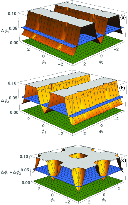
Figure 3: (Color online) The phase sensitivity varies with both phases for given $r=1.2$, and $\left|z\right|=20$. (a) The phase sensitivity of the $\phi_{1}$. (b) The phase sensitivity of the $\phi_{2}$. (c) The total phase sensitivity of both $\phi_{1}$ and $\phi_{2}$. The blue plane represents the SNL, while the green plane indicates the HL.

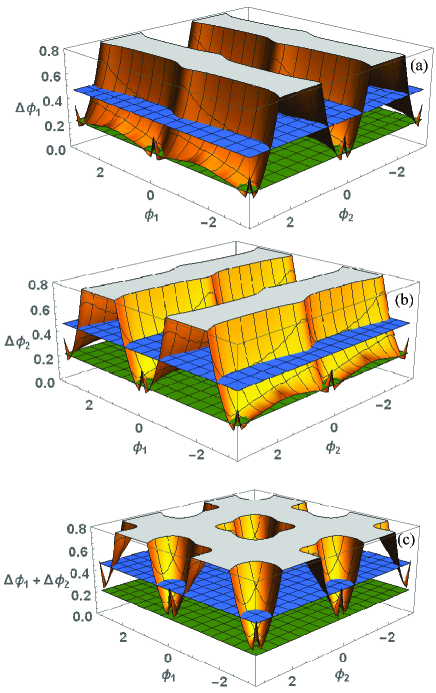
Figure 4: (Color online) The phase sensitivity varies with both phases for given $r=1.2$ and $\left|z\right|^{2}=\sinh^{2}r$. (a) The phase sensitivity of the $\phi_{1}$. (b) The phase sensitivity of the $\phi_{2}$. (c) The total phase sensitivity of both estimated phases. The blue plane represents the SNL, while the green plane indicates the HL.

In order to see clearly the varies of the phase sensitivity with respected to the phase, according to Fig. 3 (a) and Fig. 4 (a), we plot the phase sensitivity as a function of one phase $\phi_{i}$ in Fig. 5 when the other phase (for example, $\phi_{2}=0$) around zero. One see again that although the optimal working points of the phases are not zero, they are very close to zero. For a given squeezing parameter, the phase sensitivity of one phase shift is basically unchanged throughout the phase space when the intensity of the coherent state is large enough. In general, although the phase sensitivity can not surpass the HL, it can still surpass the SNL as shown in Fig. 5 (a). On the other hand, in the case of $\left|z\right|^{2}=\sinh^{2}r$, the phase sensitivity can surpass the HL for a small range of the phase as shown in Fig. 5 (b).

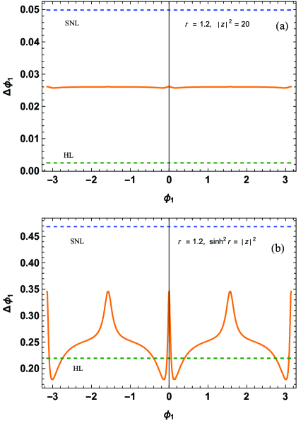
Figure 5: (Color online) The phase sensitivity varies with the phase shift $\phi_{1}$ for given $\phi_{2}=0$, and $r=1.2$. (a) $\left|z\right|^{2}=20$. (b) $\left|z\right|^{2}=\sinh^{2}r$. The blue dashed line represents the SNL, while the green dashed line indicates the HL.

At the phase point $\phi_{1}=\phi_{2}=0$, we plot the phase sensitivity versus the average total photon number of the input state in Fig. 6. We can see that the SVS can further improve the phase sensitivity within a constraint on the total photon number in the interferometer. In the case of $r=0$, the CRB saturates the QCRB as shown in Fig. 6 (a). For a given values of the squeezing parameter $r$, when $\left|z\right|^{2}\gg\sinh^{2}r$, i.e., the intensity of the coherent state is large enough, the CRB can asymptotically approach the QCRB too. Therefore, although the double-port homodyne detection is not the optimal measurement, it is still a quasi-optimal scheme.

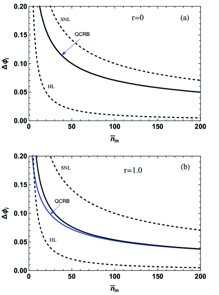
Figure 6: (Color online)  Phase sensitivity versus the average total photon number of the input state for given values of the squeezing parameter $r$. (a) $r=0\,$. (b) $r=1.0$. The upper black dashed line denotes the SNL, while the below black dashed line represents the HL. line represents the HL.

On the other hand, for the phase shift generated only in one mode of the MZI, the CRB defined by $\sqrt{1/F_{ii}^{c}}$ in the case of $\phi=0$ reads

$$\left(\Delta^{2}\phi\right)_{\text{CRB}}=\frac{1}{\left|z\right|^{2}\left(1+e^{2r}\right)},$$ (37)

which is consistent with that results in Refs. [51, 53]. Comparing Eq. (37) with Eq. (15), one can clearly see that the CRB of the single-phase estimation also does not saturate the QCRB. It should be pointed out that, for the phase shift generated only in one mode of the MZI, the optimal working points of the phase is also not zero, but very close to zero. Similarly, by numerical analysis, it shows that the optimal working points of the phase also depends on these parameter of the input state.

Conclusions

In summary, we have proposed a double-port homodyne detection to realized two-parameter estimation in a squeezing-light MZI. According to the model and basic theory of the general MZI with two-phase model, the measurement signal of the homodyne detection is not only depended on the phase difference, but also depended on the phase sum between the two arms of the interferometer. Therefore, we can obtain the two phase shifts $\phi_{1}$ and $\phi_{2}$ simultaneously by the double-port homodyne detection. Via the QFIM, our results show that the ultimate phase sensitivity, the QCRB, of the estimated phase can be improved by the SVS, and can surpass the SNL, even surpass the HL when half of the input intensity of the interferometer is provided by the coherent state and half by the squeezed light. According to the CFIM, the phase sensitivity of one estimated phase obtained by the double-port homodyne detection can beat the SNL, and can be improved by the SVS. Particularly, when the intensity of the coherent state is much larger than that of the SVS, the phase sensitivity of the estimated phase will asymptotically approach the QCRB. On the other hand, when half of the input intensity of the interferometer is provided by the coherent state and half by the squeezed light, the phase sensitivity of one estimated phase can even surpass the HL for a small range of the phase. Although, for two-parameter estimation in a squeezed-light MZI, the double-port homodyne detection is not the optimal measurement, it is still a quasi-optimal scheme. In addition, our method for two-parameter estimation with single MZI may also be applicable to other probe states.

Declaration of Competing Interest

The authors declare that they have no known competing financial interests or personal relationships that could have appeared to influence the work reported in this paper.

Data availability.

No data were generated or analyzed in the presented research.

References

- [1] V. Giovannetti, S. Lloyd, and L. Maccone, Science, 306, 1330 (2004).
- [2] C. W. Helstrom, Quantum Detection and Estimation Theory (Academic, New York, 1976), Chap.8.
- [3] C. M. Caves, ”Quantum-mechanical noise in an interferometer,” Phys. Rev. D 23, 1693–1708 (1981).
- [4] B. Yurke, S. L. McCal, and J. R. Klauder, ”SU(2) and SU(1,1) interferometers,” Phys. Rev. A 33, 4033–4054 (1986).
- [5] S. L. Braunstein and C.M. Caves, Phys. Rev. Lett. 72, 3439 (1994).
- [6] S. L. Braunstein, ”Quantum limits on precision measurements of phase,” Phys. Rev. Lett. 69, 3598–3601 (1992).
- [7] M. J. Holland and K. Burnett,”Interferometric detection of optical phase shifts at the Heisenberg limit,” Phys. Rev. Lett. 71, 1355–1358 (1993).
- [8] J. P. Dowling,”Quantum optical metrology-the lowdown on high-NOON states,” Contemp. Phys. 49, 125–143 (2008).
- [9] P. M. Anisimov, G. M. Raterman, A. Chiruvelli,W. N. Plick, S. S. Huver, H. Lee, and J. P. Dowling, ”Quantum metrology with two-mode squeezed vacuum: parity detection beats the Heisenberg limit,” Phys. Rev. Lett. 104, 103602 (2010).
- [10] J. Joo, W. J. Munro, and T. P. Spiller, ”Quantum metrology with entangled coherent states,” Phys. Rev. Lett. 107, 083601 (2011).
- [11] S. Y. Lee, C. W. Lee, J. Lee, and H. Nha, ”Quantum phase estimation using path-symmetric entangled states,” Sci. Rep. 6, 30306 (2016).
- [12] Y. Ouyang, S. Wang, and L. Zhang, ”Quantum optical interferometry via the photon added two-mode squeezed vacuum states,” J. Opt. Soc. Am. B 33, 1373–1381 (2016).
- [13] S.Wang, X. X. Xu, Y. J. Xu, and L. J. Zhang, ”Quantum interferometry via a coherent state mixed with a photon-added squeezed vacuum state,” Opt. Commun. 444, 102–110 (2019).
- [14] N. Samantary, I. Ruo-Berchera, and I.P. Degiovanni, ”Single-phase and correlated phase estimation with multiphoton annihilated squeezed vacuum state: An energy-balancing scenario,” Phys. Rev. A 101, 063810 (2020).
- [15] Y. Gao, ”Quantum optical metrology in the lossy SU(2) and SU(1,1) interferometers,” Phys. Rev. A 94, 023834 (2016).
- [16] Q. K. Gong, X. L. Hu, D. Li, C. H. Yuan, Z. Y. Ou, and W. Zhang, ”Intramode-correlation-enhanced phase sensitivities in an SU(1,1) interferometer,” Phys. Rev. A 96, 033809 (2017).
- [17] D. Li, B. T. Gard, Y. Gao, C. H. Yuan, W. Zhang, H. Lee, and J. P. Dowling, ”Phase sensitivity at the Heisenberg limit in an SU(1,1) interferometer via parity detection,” Phys. Rev. A 94, 063840 (2016).
- [18] D. Li, C. H. Yuan, Y. Yao, W. Jiang, M. Li, and W. Zhang, “Effects of loss on the phase sensitivity with parity detection in an SU(1,1) interferometer,” J. Opt. Soc. Am. B 35, 1080–1092 (2018).
- [19] S. Wang and J.D. Zhang, ”SU(1, 1) interferometry with parity measurement,” J. Opt. Soc. Am. B 38, 2687-2693 (2021).
- [20] L. L. Hou, J. D. Zhang, and S. Wang, ” Parity-based estimation in an SU(1,1) interferometer with photon-subtracted squeezed vacuum states,” Opt. Commun. 537, 129417 (2023).
- [21] F. Hudelist, J. Kong, C. Liu, J. Jing, Z. Y. Ou, and W. Zhang, ”Quantum metrology with parametric amplifierbased photon correlation interferometers,” Nat. Commun. 5, 3049 (2014).
- [22] M. Manceau, G. Leuchs, F. Khalili, and M. Chekhova, ”Detection loss tolerant supersensitive phase measurement with an SU(1,1) interferometer,” Phys. Rev. Lett. 119, 223604 (2017).
- [23] Jens A.H. Nielsen, Jonas S. Neergaard-Nielsen, Tobias Gehring, and Ulrik L. Andersen, Deterministic quantum phase estimation beyond N00N states, Phys. Rev. Lett. 130, 123603 (2023).
- [24] J. Qin, Y. H. Deng, H. S. Zhong, L. C. Peng, H. Su, Y. H. Luo, J. M. Xu, D. Wu, S. Q. Gong, H. L. Liu, H. Wang, M. C. Chen, L. Li, N. L. Liu, C. Y. Lu, and J. W. Pan, Unconditional and robust quantum metrological advantage beyond N00N states, Phys. Rev. Lett. 130, 070801 (2023).
- [25] P. C. Humphreys, M. Barbieri, A. Datta, and I. A.Walmsley, ”Quantum enhanced multiple phase estimation,” Phys. Rev. Lett. 111, 070403 (2013).
- [26] J. D. Yue, Y. R. Zhang, and H. Fan, ” Quantum enhanced metrology for multiple phase estimation with noise,” Sci. Rep. 4, 5933 (2014).
- [27] L. B. Ho, H. Hakoshima, Y. Matsuzaki, M. Matsuzaki, and Y. Kondo, ”Multiparameter quantum estimation under dephasing noise,” Phys. Rev. A 102, 022602 (2020).
- [28] Y. Yao, L. Ge, X. Xiao, X. G. Wang, and C. P. Sun, ”Multiple phase estimation for arbitrary pure states under white noise,” Phys. Rev. A 90, 062113 (2014).
- [29] S. L. Hong, J. Rehman, Y. S. Kim, Y. W. Cho, S. W. Lee, H. Jung, S. Moon, S. W. Han, and H. T. Lim, ”Quantum enhanced multiple-phase estimation with multi-mode NOON states,” Nat. Commun. 12, 5211 (2021).
- [30] J. Liu, X. M. Lu, Z. Sun, and X. G. Wang, ” Quantum multiparameter metrology with generalized entangled coherent state,” J. Phys. A 49, 115302 (2016).
- [31] Z. B. Hou, R. J. Wang, J. F. Tang, H. D. Yuan, G. Y. Xiang, C. F. Li, and G. C. Guo, ” Control-enhanced sequential scheme for general quantum parameter estimation at the Heisenberg limit,” Phys. Rev. Lett. 123, 040501 (2019).
- [32] H. Kwon, Y. Lim, L. Jiang, H. Jeong, and C. Oh, ”Quantum metrological power of continuous-variable quantum networks,”Phys. Rev. Lett. 128, 180503 (2022).
- [33] S. S. Pang and A. N. Jordan, ”Optimal adaptive control for quantum metrology with time-dependent Hamiltonians,” Nat. Commun. 8, 14695 (2017).
- [34] J. Yang, S. S. Pang, Y. Y. Zhou, and A. N. Jordan, ”Optimal measurements for quantum multiparameter estimation with general states,” Phys. Rev. A 100, 032104 (2019).
- [35] R. Nichols, P. Liuzzo-Scorpo, P. A. Knott, and G. Adesso, ”Multiparameter Gaussian quantum metrology,” Phys. Rev. A 98, 012114 (2018)
- [36] L. Pezzé M. A. Ciampini, N. Spagnolo, P. C. Humphreys, A. Datta, I. A. Walmsley, M. Barbieri, F. Sciarrino, and A. Smerzi, ”Optimal measurements for simultaneous quantum estimation of multiple phases,” Phys. Rev. Lett. 119, 130504 (2017).
- [37] W. Ge, K. Jacobs, Z. Eldredge, A. V. Gorshkov, and M. Foss-Feig, ”Distributed quantum metrology with linear networks and separable inputs,” Phys. Rev. Lett. 121, 043604 (2018).
- [38] Z. B. Hou, J. F. Tang, H. Z. Chen, H. D. Yuan, G. Y. Xiang, C. F. Li, and G. C. Guo, ”Zero-trade-off multiparameter quantum estimation via simultaneously saturating multiple Heisenberg uncertainty relations,” Sci. Adv. 7, eabd2986 (2021).
- [39] L. Zhang and K. W. C. Chan, ”Quantum multiparameter estimation with generalized balanced multimode NOON like states,” Phys. Rev. A 95, 032321 (2017).
- [40] H. Zhang, W. Ye, S. Chang, Y. Xia, L. Hu, and Z. Liao, ”Quantum multiparameter estimation with multimode photon catalysis entangled squeezed state,” Front. Phys. 18, 42304 (2023).
- [41] M. Luo, Y. Chen, J. Liu, S. Ru, and S. Gao, ” Enhancement of phase sensitivity by the additional resource in a Mach-Zehnder interferometer,” Phys. Lett. A, 424, 127823 (2022).
- [42] M. A. Taylor and W. P. Bowen, ”Quantum metrology and its application in biology,” Phys. Rep. 615, 1 (2016).
- [43] N. P. Mauranyapin, L. S. Madsen, M. A. Taylor, M. Waleed, and W. P. Bowen,”Evanescent single-molecule biosensing with quantum-limited precision,” Nat. Photonics 11, 477–481 (2017).
- [44] M. A. Taylor, J. Janousek, V. Daria, J. Knittel, B. Hage, H. A. Bachor, and W. P. Bowen, ”Biological measurement beyond the quantum limit,” Nat. Photonics 7, 229–233 (2013).
- [45] M. Genovese, ”Real applications of quantum imaging,” J. Opt. 18, 073002 (2016).
- [46] L. J. Fiderer, T. Tufarelli, S. Piano, and G. Adesso, ”General expressions for the quantum Fisher information matrix with applications to discrete quantum imaging,” PRX Quantum 2, 020308 (2021).
- [47] C. Lupo, Z. X. Huang, and P. Kok, ”Quantum limits to incoherent imaging are achieved by linear interferometry,” Phys. Rev. Lett. 124, 080503 (2020).
- [48] M. D. Vidrighin, G. Donati, M. G. Genoni, X. M. Jin, W. S. Kolthammer, M. S. Kim, A. Datta, M. Barbieri, and I. A. Walmsley. ”Joint estimation of phase and phase diffusion for quantum metrology,” Nat. Commun. 5, 3532 (2014).
- [49] F. Yao, Y.M. Du, H. Xing, and L. Fu, ” Two-parameter estimation with three-mode NOON state in a symmetric triple-well potential,” Commun. Theor. Phys. 74, 045103 (2022).
- [50] O. Steuernagel and S. Scheel, Approaching the Heisenberg limit with two-mode squeezed states, J. Opt. B 6, S66 (2004).
- [51] C. Oh, S. Y. Lee, H. Nha, and H. Jeong, Practical resources and measurements for lossy optical quantum metrology, Phys. Rev. A 96, 062304 (2017).
- [52] W. Zhong, L. Zhou, and Y. B. Sheng, Double-port measurements for robust quantum optical metrology, Phys. Rev. A 103, 042611 (2021).
- [53] L. Zhou, P. Liu, and G. R. Jin, Double-port homodyne detection in a squeezed-state interferometry with a binary-outcome data processing, Commun. Theor. Phys. 74, 125104 (2022)
- [54] Y. Jo, S. Lee, Y. S. Ihn, Z. Kim, and S. Y. Lee, Quantum illumination receiver using double homodyne detection, Phys. Rev. R. 3, 013006 (2021).
- [55] M. Jarzyna and R. Demkowicz-Dobrzański, ” Quantum interferometry with and without an external phase referenc,” Phys. Rev. A 85, 011801(R) (2012).
- [56] Scully M O, Zubairy S. Quantum optics, Cambridge University Press, 1997.
- [57] M. Jarzyna and R. Demkowicz-Dobrzański, ” Quantum interferometry with and without an external phase referenc,” Phys. Rev. A 85, 011801(R) (2012).
- [58] M. Takeoka, K. P. Seshadreesan, C. You, S. Izumi, and J. P. ” Dowling, Fundametal precision limit of a Mach-Zehnder interferometric sensor when one of the inputs is the vacuum,” 96, 052118 (2017).
- [59] Q. K. Gong, D. Li, C. H. Yuan, Z. Y. Ou, and W. P. Zhang, ”Phase estimation of phase shifts in two arms for an SU(1,1) interferometer with coherent and squeezed vacuum states,” Chin. Phys. B 26, 094205 (2017).
- [60] C. You, S. Adhikari, X. P. Ma, M. Sasaki, M. Takeoka, and J. P. Dowling, ”Conclusive precision bounds for SU(1, 1) interferometers,” Phys. Rev. A 99, 042122 (2019).
- [61] S. M. Kay, Fundamentals of Statistical Signal Processing,Volume I: Estimation Theory, 1st ed. (Prentice Hall, Englewood Cliffs, N.J, 1993).
- [62] H. Y. Fan, General formalism for mapping of two-mode classical canonical transformations to quantum unitary operators, Commun. Theor. Phys. 17, 355-360 (1992).