A Two-Stage 2D Channel Extrapolation Scheme for TDD 5G NR Systems

Abstract

Recently, channel extrapolation has been widely investigated in FDD massive MIMO systems. However, in TDD 5G new radio (NR) systems, the channel extrapolation problem also arises due to the hopping uplink pilot pattern, which has not been fully researched yet. This paper addresses this gap by formulating a channel extrapolation problem in TDD massive MIMO-OFDM systems for 5G NR, incorporating imperfection factors. A novel two-stage 2D channel extrapolation scheme in frequency-time domain is proposed, designed to mitigate the effects of imperfection factors and ensure high-accuracy channel estimation. Specifically, in the channel estimation stage, we propose a novel multi-band multi-timeslot based high-resolution parameter estimation algorithm to achieve 2D channel extrapolation in the presence of imperfection factors. Then, to avoid repeated multi-timeslot channel estimation, a channel tracking stage is designed during the subsequent time instants, where a sparse Markov channel model is formulated to capture the dynamic sparsity of massive MIMO-OFDM channels under the influence of imperfection factors. Next, an expectation-maximization (EM) based compressive channel tracking algorithm is designed to estimate unknown imperfection and channel parameters by exploiting the high-resolution prior information of the delay/angle parameters from previous timeslots. Simulation results underscore the superior performance of our proposed channel extrapolation scheme over baselines.

I Introduction

Massive multiple input multiple output (MIMO) presents a viable technology in fifth-generation (5G) New Radio (NR) systems, capable of utilizing substantial spatial multiplexing gain to satisfy escalating demands for large communication capacity [1, 2]. Yet, the deployment of massive MIMO communication systems hinges on obtaining precise channel state information (CSI) at the base station (BS), which is a challenge for a practical time-varying wireless channel subject to system imperfections.

In time division duplex (TDD) massive MIMO systems, the BS can efficiently estimate downlink channels based on the received uplink pilots (also called Sounding Reference Signals (SRSs) in 5G NR systems [3]) transmitted from the user due to channel reciprocity. As compared to frequency division duplex (FDD) systems, TDD systems drastically reduce the pilot overhead for CSI acquisition at the BS. However, owing to the user’s limited transmission power, the user typically transmits the SRSs within a bandwidth part (BWP), occupying only a fraction of the entire system bandwidth for a given SRS period [3]. Different timeslots adopt a frequency hopping pattern, depicted in Fig. 1, where the blue part denotes the time-frequency resource block occupied by the SRS symbols, with a total of $h_{p}$ hops, e.g., $h_{p}=4$ in Fig. 1. This approach ensures that the power spectral density per subcarrier of the transmitted SRSs surpasses that of a full-band SRSs transmission scheme, enhancing the transmission system’s anti-noise interference capability. However, this method estimates only a subset of the uplink channels in the time-frequency domain using received SRSs, necessitating the extrapolation method to deduce the remaining channels.

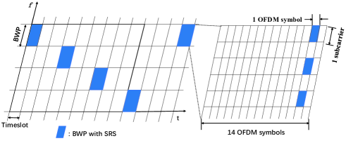
Figure 1: An illustration of the hopping SRS pattern.

Numerous channel estimation/extrapolation methodologies have been proposed in massive MIMO systems. Traditional methods such as the least square (LS) approach [4] and minimum mean square error (MMSE) method [5, 6] have been widely employed, but their extrapolation capabilities are limited. Conversely, high-resolution parameter estimation (HRPE) algorithms, which estimate the multipath components (MPCs), can achieve wide frequency range channel extrapolation, e.g., subspace-based algorithms [7, 8], compressed sensing (CS) methods [9], and etc. A significant volume of research has explored channel extrapolation in the frequency domain of the FDD systems, e.g., [6, 10, 11, 8], which extrapolates the uplink channel to the downlink channel by leveraging their pronounced spatial correlations. This correlation exists because signals at different frequencies propagate within the same environment and follow identical propagation paths [12]. Consequently, this approach eliminates the overhead associated with pilot transmission and feedback for the downlink channel [13]. In [6], the authors analyzed the theoretical performance bound of channel extrapolation in FDD massive MIMO systems. In [11], machine learning methods have been applied to extrapolate downlink CSI from observed uplink CSI in MIMO systems. The channel extrapolation in time domain has also been examined, e.g., [14, 15], and a multi-domain channel extrapolation scheme has been proposed in [16].

Nevertheless, there are limitations of the existing work:

(i) Few studies have explored channel extrapolation in TDD massive MIMO systems, focusing more on FDD systems. However, in FDD systems, pilots are uniformly assigned across the entire system bandwidth and additional pilots are usually transmitted in the downlink to estimate the channel path coefficients since the uplink and downlink channels in FDD do not share the same channel path coefficients. As a result, the existing channel extrapolation schemes for FDD systems cannot work in TDD 5G NR systems that need to estimate both delay/angle parameters and channel path coefficients from the frequency hopping pilots.

(ii) Most research only conducts one-dimensional channel extrapolation in frequency or time domain. Moreover, the imperfection factors such as the Doppler frequency offset, time offset, and random phase noise in real systems [17, 18], distort the time correlation of the channel, which further complicates channel extrapolation in both time and frequency domains.

Motivated by the limitations of existing channel extrapolation methods and the challenges brought by the imperfection factors, this paper considers a TDD massive MIMO-OFDM scenario, bearing in mind the practical imperfections in 5G NR systems. We propose a novel two-stage 2D channel extrapolation scheme that operates in both frequency and time domain. This scheme is compatible with 5G NR and can circumvent all imperfections to achieve high-accuracy channel parameter estimation. The main contributions of this paper are summarized as follows.

1. We propose a novel two-stage 2D channel extrapolation scheme, including a new extrapolation signal model for TDD 5G NR systems and a two-stage channel extrapolation algorithm. The signal model designed for 2D channel extrapolation is time-variant and considers a hopping pilot pattern and multiple imperfection factors in real 5G NR systems. In the first stage, we perform a multi-band multi-timeslot channel estimation by combining the received SRS observations from multiple timeslots and distinct BWPs to realize a 2D channel extrapolation. Subsequently, for the sake of keeping the CSI fresh and accurate, meanwhile, avoiding huge complexities caused by frequent multi-timeslots based channel estimation, we perform channel extrapolation in the following timeslots using channel tracking methods in the second stage by exploiting high-resolution prior information of channel parameters passed from the previous timeslot.

2. In the first stage (channel estimation stage), we propose a multi-band multi-timeslot HRPE (MBMT-HRPE) scheme based on a novel robust time-space-time multiple signal classification (R-TST-MUSIC) algorithm, which is an extension of the TST-MUSIC [19] from single-band/single-timeslot to multi-band and multi-timeslot. Unlike traditional single-band or single-timeslot based MUSIC algorithm, which cannot achieve HRPE due to the effect of imperfection factors, our proposed R-TST-MUSIC algorithm is able to coherently combine observations from various timeslots and BWPs to obtain equivalent full-band observations by compensating for the time-variant imperfection factors, thereby achieving high-accuracy parameter estimation. Specifically, following algorithm initialization, the proposed R-TST-MUSIC algorithm performs alternating optimization (AO) iterations between three components: Multi-band observations splicing; Joint delay-angle channel parameters estimation using a TST-MUSIC-SIC method (a combination of the TST-MUSIC and successive interference cancellation); Imperfection factors and channel coefficients estimation based on the maximum likelihood (ML) method. Such a MBMT-HRPE stage is crucial because channel extrapolation has a very high requirement on the delay estimation accuracy. Therefore, it is necessary for the initial stage to provide a high-resolution prior information of the delay parameters for the subsequent tracking stage.

3. In the second stage (channel tracking stage), a sparse Markov channel model is developed to capture the time correlation and sparsity of the massive MIMO-OFDM channels while considering imperfection factors. Then, a robust channel tracking scheme is proposed to achieve channel extrapolation at each timeslot based on expectation-maximization (EM) method. During the E-Step, we employ the dynamic Turbo-CS method and message passing method to leverage the time correlation and sparsity of the channel to accomplish Bayesian channel estimation. Then, in the M-Step, given the Bayesian channel estimation results and the high-resolution prior information from the previous timeslot, both delay/angle off-grid and imperfection parameters are estimated to further enhance the channel extrapolation accuracy and the robustness against system imperfections.

The rest of this paper is organized as follows. In Section II, we describe the system and signal model. In Section III and IV, we present the proposed channel extrapolation scheme in the channel estimation stage and the channel tracking stage, respectively. Finally, the simulation results and conclusions are given in Sections V and VI, respectively.

Notations: The notation $\left\|\cdot\right\|_{F}$ denotes the Frobenius norm, $\angle(\cdot)$ denotes the phase of a complex scalar, $vec(\cdot)$ denotes the vectorization, $\mathrm{diag}\left(\cdot\right)$ constructs a diagonal matrix from its vector argument, $\odot$, $\otimes$, and $\ast$ denote the Khatri-Rao product, Kronecker product, and Hadamard product, respectively. The transpose, conjugate transpose, and inverse are denoted by $(\cdot)^{T},(\cdot)^{H},(\cdot)^{-1}$ respectively. $\mathcal{CN}(\mathbf{x};\mathrm{\boldsymbol{\mu}},\boldsymbol{\Sigma})$ denotes a complex Gaussian normal distribution corresponding to variable $\mathbf{x}$ with mean $\boldsymbol{\mu}$ and covariance matrix $\boldsymbol{\Sigma}$.

II System and Signal Model

II-A System Model

We consider a TDD massive MIMO-OFDM system, where each single antenna user transmits uplink hopping SRSs and moves with low speed. The SRSs have been specified in the 3GPP 5G NR Release 16, which is obtained from Zadoff-Chu (ZC) sequence [3]. Note that the extension of our scenario to a user with multiple antennas is trivial, since the antennas in the same user are generally assigned with orthogonal SRSs. Moreover, since different users in the same cell transmit SRSs at different subcarriers/OFDM symbols, we focus on the channel extrapolation problem for a single user in this paper. The BS is equipped with $N_{r}=N_{x}\times N_{y}$ uniform planar array (UPA) antennas, where $N_{x}$ and $N_{y}$ represent the antenna number in the horizontal and vertical direction, respectively.

In 5G NR systems, a timeslot contains 14 OFDM symbols. To save pilot overhead and improve the spectrum efficiency, the SRS is periodically transmitted at the consecutive 1, 2 or 4 OFDM symbols in a timeslot with the period of $T_{S}$ timeslots [3]. In frequency domain, the SRS pattern for a user has a comb structure in its allocated BWP, i.e., the SRS is transmitted on every $N_{c}$ subcarrier in the BWP. Without loss of generality, we focus on the comb-2 mode in this paper, i.e., $N_{c}=2$, and the SRS symbols are transmitted at 1 OFDM symbol in a timeslot, as shown in Fig. 1.

II-B Signal Model

In the $t$-th SRS symbol, the channel frequency response (CFR) at the $n$-th ($0\leq n\leq N-1$) subcarrier is given by

$$\mathbf{h}^{(t)}\left[n\right] =e^{j\varepsilon^{(t)}}\!\!\sum_{k=1}^{K^{(t)}}\!\alpha_{k}^{(t)}e^{j\varphi_{k}^{(t)}}\!e^{-j2\pi nf_{s}\left(\tau_{k}^{(t)}+\tau_{0}^{(t)}\right)}\!\boldsymbol{a}_{R}\!\left(\!\theta_{k}^{(t)},\phi_{k}^{(t)}\!\right),$$ (1)

where $K^{(t)}$ is the number of propagation paths, $f_{s}$ denotes the subcarrier spacing, $\alpha_{k}^{(t)}$, $\theta_{k}^{(t)}$, $\phi_{k}^{(t)}$, and $\tau_{k}^{(t)}$ denote the complex path gain, azimuth angle of arrival (AoA), elevation AoA and time delay of the $k$-th path, respectively. The notations $\varphi_{k}^{(t)}$ , $\varepsilon^{(t)}$, and $\tau_{0}^{(t)}$ denote the imperfection factors, i.e., Doppler phase rotation factor caused by user mobility, random phase noise, and the time offset [17, 18]. Without loss of generality, we set $\varepsilon^{(1)}=0,\tau_{0}^{(1)}=0,\varphi_{k}^{(1)}=0,\forall k,$ for the first SRS symbol. The factor $\varphi_{k}^{(t)}$ depends on the Doppler frequency offset $f_{D,k}^{(t)}$ as $\varphi_{k}^{(t)}=\varphi_{k}^{(t-1)}+2\pi T_{SRS}f_{D,k}^{(t)}$, where $T_{SRS}$ is the time interval between two adjacent SRS symbols. Since we focus on the scenario with a low-speed and acceleration of the user, $f_{D,k}^{(t)}$ varies slowly and has a strong time-correlation to be exploited. $\boldsymbol{a}_{R}\left(\theta,\phi\right)=\boldsymbol{a}_{x}\left(\theta,\phi\right)\otimes\boldsymbol{a}_{y}\left(\theta\right)\in\mathbb{C}^{N_{r}\times 1}$ is the array response vector for the BS antenna array. With half-wavelength spacing, the $n_{x}$-th element in the steering vector $\boldsymbol{a}_{x}\left(\theta,\phi\right)$ and the $n_{y}$-th element in the steering vector $\boldsymbol{a}_{y}\left(\theta\right)$ can be respectively expressed as $\left[\boldsymbol{a}_{x}\left(\theta,\phi\right)\right]_{n_{x}}=\frac{1}{\sqrt{N_{x}}}e^{j\pi n_{x}sin\left(\theta\right)cos\left(\phi\right)},\left[\boldsymbol{a}_{y}\left(\theta\right)\right]_{n_{y}}=\frac{1}{\sqrt{N_{y}}}e^{j\pi n_{y}cos\left(\theta\right)},$ with $n_{x}=0,...,N_{x}-1$ and $n_{y}=0,...,N_{y}-1$ [20].

Let $P$ denote the number of SRS subcarriers in a BWP. Then, the received frequency domain SRSs $\mathbf{Y}^{(t)}\in\mathbb{C}^{P\text{\texttimes}N_{r}}$ in a BWP for the $t$-th SRS symbol is given by

$$\mathbf{Y}^{(t)} =\textrm{diag}\left(\mathbf{x}\right)\mathbf{W}^{(t)}\mathbf{H}^{(t)}+\mathbf{N}^{(t)},$$ (2)

where $\mathbf{x}\in\mathbb{C}^{P\text{\texttimes}1}$ is the frequency domain SRSs transmitted from the user, $\mathbf{W}^{(t)}\in\left\{0,1\right\}^{P\times N}$ is a selection matrix depending on the hopping SRS pattern, e.g., $\mathrm{W^{(1)}}\left(i,j\right)=1$ for $j=2i-1$, $i=1,...,P$, $\mathbf{H}^{(t)}\triangleq[(\mathbf{h}^{(t)}[0])^{T};(\mathbf{h}^{(t)}[1])^{T};...;(\mathbf{h}^{(t)}[N-1])^{T}]\in\mathbb{C}^{N\times N_{r}}$ denotes the CFR matrix on the full-band, and $\mathbf{N}^{\left(t\right)}$ is the additive white Gaussian noise (AWGN) with each element having zero mean and variance $\sigma_{e}^{(t)}$.

III Channel Extrapolation in Channel Estimation Stage

In this section, we aim to achieve a 2D channel extrapolation based on the received hopping SRSs, as illustrated in Fig. 2. We first reformulate the received signal model and give an overview of the TST-MUSIC algorithm. Nevertheless, the original TST-MUSIC algorithm cannot use the multi-timeslot multi-band observations in a coherent way due to the effect of imperfection factors, which motivates the proposed R-TST-MUSIC algorithm.

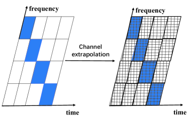
Figure 2: Channel extrapolation in channel estimation stage.

III-A Review of TST-MUSIC Algorithm

we reformulate the received signal model (2) as:

$$\mathbf{Y}^{(t)}=\mathbf{G}^{(t)}\left(\boldsymbol{\tau}+\tau_{0}^{(t)}\right)\mathbf{B}\mathbf{A}\left(\theta,\phi\right)^{T}+\mathbf{N}^{(t)},$$ (3)

where $\mathbf{A}\left(\theta,\phi\right)=[\boldsymbol{a}_{R}(\theta_{1}^{(t)},\phi_{1}^{(t)}),...,\boldsymbol{a}_{R}(\theta_{K^{(t)}}^{(t)},\phi_{K^{(t)}}^{(t)})]\in\mathbb{C}^{N_{r}\times K^{(t)}}$, $\mathbf{B}=\textrm{diag}(\widetilde{\alpha}_{1}^{(t)},...,\widetilde{\alpha}_{K^{(t)}}^{(t)})$ with $\widetilde{\alpha}_{k}^{(t)}=\alpha_{k}^{(t)}e^{j\varphi_{k}^{(t)}}e^{j\varepsilon^{(t)}}$, $\mathbf{G}^{(t)}(\boldsymbol{\tau}+\tau_{0}^{(t)})=\textrm{diag}(\mathbf{x})\mathbf{W}^{(t)}\mathbf{F}(\boldsymbol{\tau}+\tau_{0}^{(t)})\triangleq[\mathbf{g}^{(t)}(\tau_{1}^{(t)}+\tau_{0}^{(t)}),...,\mathbf{g}^{(t)}(\tau_{K^{(t)}}^{(t)}+\tau_{0}^{(t)})]\in\mathbb{C}^{P\times K^{(t)}},\mathbf{F}(\boldsymbol{\tau}+\tau_{0}^{(t)})=[\mathbf{a}(\tau_{1}^{(t)}+\tau_{0}^{(t)}),...,\mathbf{a}(\tau_{K^{(t)}}^{(t)}+\tau_{0}^{(t)})]$ with $\mathbf{a}(\tau)=[1,\ldots,e^{-j2\pi(N-1)f_{s}\tau}]^{T}\in\mathbb{C}^{N\times 1}$. Since the user moves with a low speed and the channel varies slowly as we considered, we mildly assume that the channel parameters are time-invariant during a small number of initial timeslots in the channel estimation stage (e.g., for $h_{p}=4,$ we set the number of timeslots of the channel estimation stage $T_{e}=h_{p}=4$), i.e., $f_{D,k}^{(t)}=f_{D,k},$ $\varphi_{k}^{(t)}=(t-1)\varphi_{k}$, $K^{(t)}=K,\tau_{k}^{(t)}=\tau_{k},\alpha_{k}^{(t)}=\alpha_{k},\theta_{k}^{(t)}=\theta_{k},\phi_{k}^{(t)}=\phi_{k},\forall t\in\left\{1,...,T_{e}\right\}$. But in the simulations, the channel observations are still generated from a practical channel model specified by 3GPP TR 38.901 without adding this assumption to fairly evaluate our proposed channel extrapolation scheme. Simulation results show that our proposed channel extrapolation scheme works well in practical scenarios though we make such an assumption in our algorithm design, as detailed in Section V.

Then, we give an overview of the TST-MUSIC algorithm, which combines T-MUSIC and S-MUSIC algorithms along with the temporal filtering techniques and the spatial beamforming techniques to jointly estimate the angles and the delays of the multipaths in a wireless channel [19]. The TST-MUSIC algorithm has the advantages of high-resolution, which can resolve paths with either very close angles or very close delays and automatically pair the estimated angles and delays. For conciseness, we omit the superscript $(t)$ and focus on a single timeslot to depict the TST-MUSIC algorithms.

Specifically, the angles and delays are estimated by the S-MUSIC and T-MUSIC algorithms, which use the covariance matrices of the rows and the columns of $\mathbf{Y}$, respectively. We perform eigendecomposition of the autocorrelation matrix of (3) as

$$\mathbf{R}^{d} = \mathbb{E}\left\{\mathbf{Y}\mathbf{Y}^{H}\right\}=\mathbf{V}_{s}^{d}\boldsymbol{\Lambda}_{s}^{d}\mathbf{V}_{s}^{d\thinspace H}+\mathbf{V}_{n}^{d}\boldsymbol{\Lambda}_{n}^{d}\mathbf{V}_{n}^{d\thinspace H},$$ (4)

$$\mathbf{R}^{s} = \mathbb{E}\left\{\mathbf{Y}^{T}\mathbf{Y}^{*}\right\}=\mathbf{V}_{s}^{s}\boldsymbol{\Lambda}_{s}^{s}\mathbf{V}_{s}^{s\thinspace H}+\mathbf{V}_{n}^{s}\boldsymbol{\Lambda}_{n}^{s}\mathbf{V}_{n}^{s\thinspace H},$$ (5)

where the column vectors of $\mathbf{V}_{s}^{d}$ and $\mathbf{V}_{s}^{s}$ are the eigenvectors that span the signal subspace of $\mathbf{R}^{d}$ and $\mathbf{R}^{s}$, respectively, corresponding to the largest $K$ eigenvalues. The number of multipaths $K$ can be estimated using the minimum descriptive length (MDL) criterion [21]. And the column vectors of $\mathbf{V}_{n}^{d}$ and $\mathbf{V}_{n}^{s}$ are the eigenvectors that span the noise subspace of $\mathbf{R}^{d}$ and $\mathbf{R}^{s}$, respectively. $\boldsymbol{\Lambda}_{s}^{d},\boldsymbol{\Lambda}_{n}^{d},\boldsymbol{\Lambda}_{s}^{s},\boldsymbol{\Lambda}_{n}^{s}$ are diagonal matrices consisting of the associated eigenvalues. Then, according to the orthogonality property between the signal and the noise subspace given by [22]

$$\mathbf{G}^{H}\mathbf{V}_{n}^{d} = \boldsymbol{O},$$ (6)

$$\mathbf{A}^{H}\mathbf{V}_{n}^{s} = \boldsymbol{O},$$ (7)

i.e., $\mathbf{g}(\tau_{k}+\tau_{0})^{H}\mathbf{V}_{n}^{d}=\mathbf{0}^{T},$$\boldsymbol{a}_{R}(\theta_{k},\phi_{k})^{H}\mathbf{V}_{n}^{s}=\mathbf{0}^{T},\forall k,$ the delays and angles can be estimated at which the following T-MUSIC and S-MUSIC pseudospectrums achieve maximum values, respectively:

$$\mathcal{P}_{\text{}}^{d}(\tau) = \frac{1}{\mathbf{g}(\tau)^{H}\left(\mathbf{I}-\mathbf{V}_{s}^{d}\mathbf{V}_{s}^{d\thinspace H}\right)\mathbf{g}(\tau)},$$ (8)

$$\mathcal{P}_{\text{}}^{s}(\theta,\phi) = \frac{1}{\boldsymbol{a}_{R}(\theta,\phi)^{H}\left(\mathbf{I}-\mathbf{V}_{s}^{s}\mathbf{V}_{s}^{s\thinspace H}\right)\boldsymbol{a}_{R}(\theta,\phi)}.$$ (9)

In summary, the TST-MUSIC algorithm has five steps:

Step 1) Grouping: Apply the T-MUSIC algorithm to obtain the group delays $\left\{\hat{t}_{1},...,\hat{t}_{q}\right\}$ based on (4) and (8).

Step 2) Temporal Filtering: The output of the $k$-th group after filtering is given by

$$\mathbf{Y}_{k}=\prod_{n=1;n\neq k}^{q}\mathbf{U}_{n}^{d}\cdot\mathbf{Y},k=1,...,q,$$ (10)

where $\mathbf{U}_{n}^{d}=\mathbf{I}-\frac{1}{P}\mathbf{g}\left(\hat{t}_{n}\right)\mathbf{g}^{H}\left(\hat{t}_{n}\right)$ are the temporal filtering matrices.

Step 3) DOA Estimation: Apply the S-MUSIC algorithm to each $\mathbf{Y}_{k}$ and estimate the angles at each group given by

$$\left(\hat{\boldsymbol{\theta}}_{k},\hat{\boldsymbol{\phi}}_{k}\right)=\left[\left(\hat{\theta}_{k,1},\hat{\phi}_{k,1}\right),...,\left(\hat{\theta}_{k,r(k)},\hat{\phi}_{k,r(k)}\right)\right]^{T},$$ (11)

where $r(k)$ is the number of paths in the $k$-th group.

Step 4) Spatial Beamforming: The output of the $m$-th spatial beamformer is given by

$$\mathbf{Y}_{k,m}=\mathbf{Y}_{k}\cdot\prod_{n=1;n\neq m}^{r(k)}\mathbf{U}_{k,n}^{s},k=1,...,K,m=1,...,r(k)$$ (12)

where $\mathbf{U}_{k,n}^{s}=\mathbf{I}-\boldsymbol{a}_{R}\left(\hat{\theta}_{k,n},\hat{\phi}_{k,n}\right)\boldsymbol{a}_{R}^{H}\left(\hat{\theta}_{k,n},\hat{\phi}_{k,n}\right)$ are the spatial beamforming matrix.

Step 5) Delay Estimation: We again employ the T-MUSIC algorithm for each $\mathbf{Y}_{k,m}$ to obtain the corresponding delays.

III-B Outline of the R-TST-MUSIC Algorithm

It is evident that TST-MUSIC cannot coherently use the BWP observations across different timeslots to perform channel extrapolation with a high-accuracy delay estimation. This limitation stems from its inability to compensate for time-variant imperfection factors. As a result, when only a fraction of observations is available at each timeslot (e.g., a quarter of the full-band observations for $h_{p}=4$), the channel extrapolation capability of TST-MUSIC is limited. However, using the multi-timeslot multi-band observations in a coherent way to achieve a high-accuracy channel extrapolation is challenging due to the following reasons: (i) The imperfection factors destroy the coherence property of the received BWP observations and thus require compensation; (ii) The original orthogonality in (6) is affected by the Doppler factors, complicating the estimation of multipath delay parameters, as elaborated in Subsection III-D2.

To overcome aforementioned challenges, we propose the R-TST-MUSIC algorithm, an enhancement of the TST-MUSIC algorithm, allowing for coherent utilization of multi-timeslot multi-band observations. Compared to the original TST-MUSIC algorithm, R-TST-MUSIC is designed to produce equivalent full-band observations by compensating for the imperfection factors, yielding superior channel extrapolation performance. The proposed R-TST-MUSIC algorithm comprises two stages: an initialization phase and a refinement estimation phase. The former focuses on the preliminary parameter estimation, utilizing the TST-MUSIC and LS algorithms. This initial process sets the stage for the refinement phase, ensuring convergence to a good solution. Armed with the preliminary findings, the refinement phase then seeks a more precise solution.

The overall R-TST-MUSIC algorithm is summarized in Algorithm 1.

Algorithm 1 R-TST-MUSIC algorithm

Input: $\mathbf{Y}^{(t)}$, AO iteration number $I_{AO}$.

Output: $\hat{\tau}_{k},\hat{\theta}_{k},\hat{\phi}_{k},\hat{\varphi}_{k},\hat{\varepsilon}^{(t)},\hat{\tau}_{0}^{(t)},t=1,...,T_{e}$.

1:  Initialization Phase:

2:  Perform TST-MUSIC algorithm based on $\mathbf{Y}^{(t)}$ to obtain the estimate $\hat{\tau}_{k}^{(t)},\hat{\theta}_{k}^{(t)},\hat{\phi}_{k}^{(t)},\forall t$.

3:  Get a LS solution $\hat{\widetilde{\boldsymbol{\alpha}}}^{(t)}$in (14).

4:  Get the estimate $\hat{\varepsilon}^{(t)},\hat{\varphi}_{k}^{(t)},\hat{\tau}_{0}^{(t)}$ in (15)-(17).

5:  Refinement Estimation Phase:

6:  for ${\color[rgb]{0,0,1}{\color[rgb]{0,0,0}j=1,\cdots,I_{AO}}}$ do

7:     Construct a compensated signal model (19).

8:     Perform TST-MUSIC-SIC algorithm to estimate delay and angle parameters denoted as $\hat{\tau}_{k},\hat{\theta}_{k},\hat{\phi}_{k}$.

9:     Get the estimate $\hat{\boldsymbol{\alpha}}^{(j+1)}$, $\hat{\varepsilon}^{(t)\thinspace(j+1)},\boldsymbol{\varphi}^{(j+1)},\hat{\tau}_{0}^{(t)\thinspace(j+1)}$ based on (24)-(27).

10:  end for

III-C Initialization Phase

At the $t$-th SRS symbol with input $\mathbf{Y}^{(t)}$, we first employ the TST-MUSIC algorithm to obtain the estimate $\hat{\tau}_{k}^{(t)},\hat{\theta}_{k}^{(t)},\hat{\phi}_{k}^{(t)}$. The signal model (3) can be reformulated as

$$\mathbf{y}^{(t)}=\mathbf{V}^{(t)}\widetilde{\boldsymbol{\alpha}}^{(t)}+\mathbf{n}^{(t)},$$ (13)

where $\mathbf{y}^{(t)}\triangleq vec(\mathbf{Y}^{(t)})\in\mathbb{C}^{N_{r}P\times 1}$, $\mathbf{V}^{(t)}=\mathbf{A}(\theta,\phi)\odot\mathbf{G}^{(t)}(\boldsymbol{\tau}+\tau_{0}^{(t)})\in\mathbb{C}^{N_{r}P\times K}$, $\mathbf{n}^{(t)}=vec(\mathbf{N}^{(t)})$, and $\widetilde{\boldsymbol{\alpha}}^{(t)}=[\widetilde{\alpha}_{1}^{(t)},...,\widetilde{\alpha}_{K}^{(t)}]^{T}$. Then, we can obtain a LS solution of $\widetilde{\boldsymbol{\alpha}}^{(t)}$ as

$$\hat{\widetilde{\boldsymbol{\alpha}}}^{(t)}=(\mathbf{V}^{(t)H}\mathbf{V}^{(t)})^{-1}\mathbf{V}^{(t)H}\mathbf{y}^{(t)}.$$ (14)

Finally, according to the inherent structure of $\widetilde{\boldsymbol{\alpha}}^{(t)}$, the imperfection parameters can be estimated as

$$\hat{\varepsilon}^{(t)} = \angle(\hat{\widetilde{\alpha}}_{1}^{(t)}/\hat{\widetilde{\alpha}}_{1}^{(1)}),$$ (15)

$$\hat{\varphi}_{k}^{(t)} = \angle\frac{\hat{\widetilde{\alpha}}_{k}^{(t)}\hat{\widetilde{\alpha}}_{1}^{(1)}}{\hat{\widetilde{\alpha}}_{k}^{(1)}\hat{\widetilde{\alpha}}_{1}^{(t)}},$$ (16)

$$\hat{\tau}_{0}^{(t)} = \frac{\sum_{k=1}^{K^{(t)}}(\hat{\tau}_{k}^{(t)}-\hat{\tau}_{k}^{(1)})}{K^{(t)}}.$$ (17)

III-D Refinement Estimation Phase

In this stage, we perform a joint multi-timeslot channel parameter estimation to achieve channel extrapolation after initialization. The proposed algorithm executes AO iterations among four components as follows.

III-D1 Step 1 (Multi-band observations splicing)

In this step, we compensate for the imperfection parameters and then splice the observation samples obtained in different BWPs into a full-band observation samples, as shown in Fig. 3.

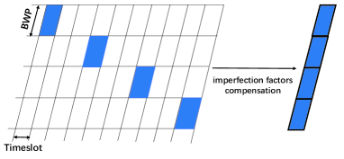
Figure 3: An illustration of step 1.

For given estimated imperfection parameters $\hat{\varepsilon}^{(t)},\hat{\varphi}_{k}^{(t)},\hat{\tau}_{0}^{(t)}$, we recover the “clean” observations as

$$\overline{\mathbf{Y}}^{(t)}=\textrm{diag}(e^{-j\hat{\varepsilon}^{(t)}})\cdot\textrm{diag}(\mathbf{W}^{(t)}\mathbf{a}(\hat{\tau}_{0}^{(t)})^{*})\cdot\mathbf{Y}^{(t)}.$$ (18)

Then, we have a compensated full-band linear signal model given by

$$\overline{\mathbf{Y}}^{(T_{e})}=\overline{\mathbf{G}}^{(T_{e})}\left(\boldsymbol{\tau}\right)\overline{\mathbf{B}}\mathbf{A}\left(\theta,\phi\right)^{T}+\mathbf{N}^{(t)},$$ (19)

where $\overline{\mathbf{Y}}^{(T_{e})}=[\overline{\mathbf{Y}}^{(1)};...;\overline{\mathbf{Y}}^{(T_{e})}]\in\mathbb{C}^{T_{e}P\times N_{r}}$, $\overline{\mathbf{G}}^{(T_{e})}(\boldsymbol{\tau})=[\overline{\mathbf{G}}^{(1)}(\boldsymbol{\tau});...;\overline{\mathbf{G}}^{(T_{e})}(\boldsymbol{\tau})]\in\mathbb{C}^{T_{e}P\times K}$ with $\overline{\mathbf{G}}^{(t)}(\boldsymbol{\tau})=\mathbf{G}^{(t)}(\boldsymbol{\tau})\textrm{diag}(e^{j\hat{\varphi}_{1}^{(t)}},...,e^{j\hat{\varphi}_{K}^{(t)}})$, and $\overline{\mathbf{B}}=\textrm{diag}(\alpha_{1},...,\alpha_{K})$.

III-D2 Step 2 (Joint delay-angle parameters estimation using TST-MUSIC-SIC)

Then, we apply the TST-MUSIC algorithm to the compensated observations $\overline{\mathbf{Y}}^{(T_{e})}$ to estimate the delay and angle parameters, but with a different T-MUSIC pseudospectrum estimation method. Particularly, the primary orthogonality property in (6) does not hold in the new full-band signal model (19) anymore due to the effect of $\hat{\varphi}_{k}^{(t)}$. Instead, we have a new orthogonality property, $\overline{\mathbf{G}}^{(T_{e})\thinspace H}\mathbf{V}_{n}^{d}=\boldsymbol{O},$ i.e., $\overline{\mathbf{g}}_{k}(\tau_{k})^{H}\mathbf{V}_{n}^{d}=\mathbf{0}^{T},\forall k$, where $\overline{\mathbf{g}}_{k}$ denotes the $k$-th column vector of $\overline{\mathbf{G}}^{(T_{e})}$. Therefore, in contrast to the primary T-MUSIC algorithm that $K$ delays are estimated based on the same pseudospectrum, in our proposed R-TST-MUSIC algorithm, $K$ delays need to be estimated based on $K$ different pseudospectrums, respectively. For instance, the delay $\tau_{k}$ can be estimated at which the pseudospectrum $\mathcal{\overline{P}}_{k}^{d}(\tau)$ derived from the signal model (19) takes the maximum value:

$$\mathcal{\overline{P}}_{k}^{d}(\tau)=\frac{1}{\overline{\mathbf{g}}_{k}(\tau)^{H}\left(\mathbf{I}-\mathbf{V}_{s}^{d}\mathbf{V}_{s}^{d\thinspace H}\right)\overline{\mathbf{g}}_{k}(\tau)},\forall k.$$ (20)

However, for the delay estimate of a certain path based on (20), the interference from other paths cannot be neglected, especially in the delay estimation of a path with low-energy. In other words, owing to the “pseudo” orthogonality, i.e., $\overline{\mathbf{g}}_{k}(\tau_{k^{\prime}})^{H}\left(\mathbf{I}-\mathbf{V}_{s}^{d}\mathbf{V}_{s}^{d\thinspace H}\right)\overline{\mathbf{g}}_{k}(\tau_{k^{\prime}})=\varepsilon,\forall k^{\prime}\neq k,$ where $\varepsilon$ has a small value, we may find a virtual delay in the vicinity of $\tau_{k^{\prime}}$. To demonstrate this phenomenon and highlight the challenges of multipaths delay estimation based on (20), we present the curves of $\mathcal{\overline{P}}_{1}^{d}(\tau)$ in Fig. 4 for estimation of delay $\tau_{1}$ , where the red circle and the red star denote the true values of $\tau_{1}$ and $\tau_{2}$, respectively. We set $K=2$, $h_{p}=4$, the true delays $\tau_{1}=40$ ns with power $-8.8$ dB, $\tau_{2}=107$ ns with power 0 dB. As depicted in Fig. 4a, two peak are observed. The first peak appears in the true value of $\tau_{1}$, following the orthogonality property. However, another peak with relatively low energy also emerges around the true value of $\tau_{2}$ due to the “pseudo” orthogonality, even if the imperfection parameters are perfectly compensated for. However, as shown in Fig. 4b when in the presence of the imperfection parameters estimation errors, the first peak deviates from the true value of $\tau_{1}$. Moreover, there is a possibility of identifying a wrong peak as the estimation result of $\tau_{1}$, since the peak with the maximum energy may no longer be located around $\tau_{1}$, but rather around $\tau_{2}$.

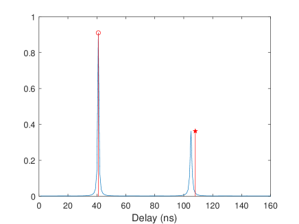
(a)

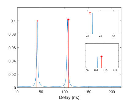
(b)

Figure 4: The pseudospectrum $\mathcal{\overline{P}}_{1}^{d}(\tau)$ in the cases: (a) Perfect imperfection parameters compensation; (b) Imperfect imperfection parameters compensation.

To solve this challenge, we adopt a successive interference cancellation (SIC) method. We first estimate the delay of the path with the largest energy ratio at which the following pseudospectrum takes the maximum value

$$\mathcal{P}_{1}^{d}(\tau)=\frac{1}{\overline{\mathbf{g}}_{1}(\tau)^{H}\left(\mathbf{I}-\mathbf{V}_{s}^{d}\mathbf{V}_{s}^{d\thinspace H}\right)\overline{\mathbf{g}}_{1}(\tau)}.$$ (21)

Without loss of generality, we have assumed that the estimated channel gains of the multipaths have a descending order, i.e., $\left|\hat{\alpha}_{k}\right|^{2}\geq\left|\hat{\alpha}_{k+1}\right|^{2},\forall k\in\left\{1,...,K-1\right\}$. Then, the contribution of the first estimated path is removed from $\overline{\mathbf{Y}}^{(T_{e})}$, i.e.,

$$\overline{\mathbf{Y}}_{1}^{(T_{e})}=\mathbf{\overline{U}}_{1}^{d}\overline{\mathbf{Y}}^{(T_{e})},$$ (22)

where $\mathbf{\overline{U}}_{1}^{d}=\mathbf{I}-\frac{1}{T_{e}P}\mathbf{\overline{g}}_{1}(\hat{\tau}_{1})\mathbf{\overline{g}}_{1}^{H}(\hat{\tau}_{1})$ denotes the temporal filtering matrix of the first path. Next, the delay of the second strongest path $\tau_{2}$ is estimated based on $\overline{\mathbf{Y}}_{1}^{(T_{e})}$, and so on. Using SIC method, finally all delays $\tau_{1},...,\tau_{K}$ are estimated in turn.

Note that in the search of the peaks of the MUSIC pseudospectrum in (21), the searching region can shrink to the vicinity of the initial delay and angle estimation results obtained from the initialization phase instead of the whole axis. Thus, the computational complexity of this step can be significantly reduced.

III-D3 Step 3 (Imperfection factors and channel coefficients estimation based on ML)

In this step, we employ ML method to estimate the imperfection parameters and the channel coefficients. The optimization problem can be formulated as

$$\mathop{\arg\min}\limits_{\varphi_{k},\varepsilon^{(t)},\tau_{0}^{(t)},\alpha_{k}}\sum\limits_{t=1}^{T_{e}}\left\|\mathbf{Y}^{(t)}-\mathbf{G}^{(t)}\left(\hat{\boldsymbol{\tau}}+\tau_{0}^{(t)}\right)\mathbf{B}\left(\alpha_{k},\varphi_{k},\varepsilon^{(t)}\right)\right.$$ (23)

$$\thinspace\thinspace\thinspace\thinspace\thinspace\thinspace\thinspace\thinspace\thinspace\thinspace\thinspace\thinspace\thinspace\thinspace\thinspace\thinspace\thinspace\thinspace\thinspace\thinspace\thinspace\thinspace\thinspace\thinspace\thinspace\thinspace\thinspace\thinspace\thinspace\thinspace\thinspace\thinspace\thinspace\thinspace\thinspace\thinspace\thinspace\thinspace\thinspace\thinspace\thinspace\thinspace\thinspace\left.\times\mathbf{A}\left(\hat{\theta}_{k},\hat{\phi}_{k}\right)^{T}\right\|_{F}^{2}.$$

Then, we use AO method to alternatively optimize the variables. Particularly, we can obtain a closed-form solution for $\alpha_{k}$ and $\varepsilon^{(t)}$ as

$$\hat{\boldsymbol{\alpha}} = ((\boldsymbol{\Psi}_{\alpha}^{(T_{e})})^{H}\boldsymbol{\Psi}_{\alpha}^{(T_{e})})^{-1}(\boldsymbol{\Psi}_{\alpha}^{(T_{e})})^{H}\mathbf{y}^{(T_{e})},$$ (24)

$$\hat{\varepsilon}^{(t)} = \angle((\boldsymbol{\Psi}_{\varepsilon}^{(t)})^{H}\mathbf{y}^{(t)}),$$ (25)

where

$$\boldsymbol{\Psi}_{\alpha}^{(T_{e})} =[\boldsymbol{\Psi}_{\alpha}^{(1)};...;\boldsymbol{\Psi}_{\alpha}^{(T_{e})}],$$

$$\!\!\boldsymbol{\Psi}_{\alpha}^{(t)} =\mathbf{A}(\theta,\phi)\!\odot\!\mathbf{G}^{(t)}(\!\boldsymbol{\tau}\!+\!\tau_{0}^{(t)}\!)\!\cdot\!\textrm{diag}(\!e^{j\varphi_{k}^{(t)}}\!e^{j\varepsilon^{(t)}}\!\!\!\!,...,e^{j\varphi_{K}^{(t)}}\!e^{j\varepsilon^{(t)}}\!),$$

$$\boldsymbol{\Psi}_{\varepsilon}^{(t)} =\mathbf{A}(\theta,\phi)\odot\mathbf{G}^{(t)}(\boldsymbol{\tau}+\tau_{0}^{(t)})\boldsymbol{\alpha}_{\varepsilon},$$

$$\boldsymbol{\alpha}_{\varepsilon} =[\alpha_{1}e^{j\varphi_{1}^{(t)}},...,\alpha_{K}e^{j\varphi_{K}^{(t)}}]^{T}.$$

Then, $\boldsymbol{\boldsymbol{\varphi}}$$\triangleq[\varphi_{1},$$...,$$\varphi_{K}]$ and $\tau_{0}^{(t)}$ can be estimated using gradient descent method as

$$\boldsymbol{\boldsymbol{\varphi}}^{(j+1)} = \boldsymbol{\boldsymbol{\varphi}}^{(j)}-\gamma_{\boldsymbol{\varphi}}\cdot\boldsymbol{\boldsymbol{\zeta}}_{\boldsymbol{\varphi}}^{(j)},$$ (26)

$$\tau_{0}^{(t)\thinspace\thinspace(j+1)} = \tau_{0}^{(t)\thinspace\thinspace(j)}-\gamma_{\tau_{0}^{(t)}}\cdot\zeta_{\tau_{0}^{(t)}}^{(j)},$$ (27)

where $\gamma_{\boldsymbol{\varphi}}$ and $\gamma_{\tau_{0}^{(t)}}$ are the step size determined by the Armijo rule [23], $\boldsymbol{\boldsymbol{\zeta}}_{\boldsymbol{\varphi}}^{(j)}$ and $\zeta_{\tau_{0}^{(t)}}^{(j)}$ are the gradients of the objective function in (23) with respect to $\boldsymbol{\boldsymbol{\varphi}}$ and $\tau_{0}^{(t)}$, respectively.

III-E Computational Complexity Analysis

The main computational complexity of R-TST-MUSIC depends on the eigendecomposition of $\mathbf{R}^{d}$ and $\mathbf{R}^{s}$ based on $\overline{\mathbf{Y}}^{(T_{e})}$, which are $\mathcal{O}\left(T_{e}^{3}P^{3}\right)$ and $\mathcal{O}\left(N_{r}^{3}\right)$, respectively, the matrix multiplication and inverse operation in (24), which are $\mathcal{O}\left(T_{e}N_{r}PK^{2}\right)$ and $\mathcal{O}\left(K^{3}\right)$, respectively. Besides, the computational complexity of the spatial and temporal searches for the S-MUSIC and T-MUSIC pseudospectrum have the orders of $\mathcal{O}\left(N_{r}^{2}g_{s}\right)$ and $\mathcal{O}\left(T_{e}^{2}P^{2}g_{t}\right)$, respectively, where $g_{s}$ and $g_{t}$ are the numbers of searches conducted along the angle axis and the delay axis.

As can be seen, the computational complexity in the channel estimation stage has a cubic order of $T_{e}$, which is unacceptable when $T_{e}$ is large. Therefore, we further propose a channel tracking based extrapolation scheme, which can exploit the time-correlation of the channel parameters and avoid frequent multi-timeslot based channel estimation.

IV Channel Extrapolation in Channel Tracking Stage

In the channel tracking stage, we aim to achieve channel extrapolation based on the received SRSs at the current time $t$ and the prior information passed from time $t-1$, as shown in Fig. 5. As compared to the one stage channel extrapolation scheme that performs multi-timeslot channel extrapolation, our proposed two-stage scheme is less time-consuming, especially for a long time channel estimation.

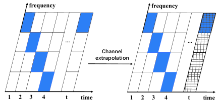
Figure 5: Channel extrapolation in channel tracking stage.

IV-A Sparse Channel Representation

We first describe sparse representation over delay and angular domain for signal model (2). One commonly used method is to define a uniform delay grid $\mathcal{D}=\{\overline{d}_{1},\ldots,\overline{d}_{L}\}$ of $L$ ($L\gg K^{(t)},\forall t$) delay points over $[-\frac{1}{4}T_{d},T_{d}]$ ($T_{d}$ denotes an upper bound for the maximum delay spread) and two uniform angle grids $\mathcal{G}_{\theta}=\{\overline{\theta}_{1},\ldots,\overline{\theta}_{N_{x}}\}$ and $\mathcal{G}_{\phi}=\{\overline{\phi}_{1},\ldots,\overline{\phi}_{N_{y}}\}$ of $N_{x}$ and $N_{y}$ angle points over $\left[0,2\pi\right]$. If all the true delay and angle values exactly lie in the discrete sets $\mathcal{D}$ and $\mathcal{G}_{\theta},\mathcal{\mathcal{G}_{\phi}}$, we can reformulate signal model (2) as

$$\mathbf{Y}^{(t)}=\textrm{diag}\left(\mathbf{x}\right)\mathbf{W}^{(t)}\boldsymbol{\Lambda}^{(t)}\mathbf{S}^{(t)}\mathbf{F}_{d}(\mathbf{H}_{d}^{(t)}\ast\mathbf{D}^{(t)})\mathbf{A}_{R}^{T}+\mathbf{N}^{(t)},$$ (28)

where $\boldsymbol{\Lambda}^{(t)}=\mathrm{diag}(e^{j\varepsilon^{(t)}},\ldots,e^{j\varepsilon^{(t)}}),$

$$\mathbf{S}^{(t)} =\mathrm{diag}(1,\ldots,e^{-j2\pi nf_{s}\tau_{0}^{(t)}},\ldots,e^{-j2\pi(N-1)f_{s}\tau_{0}^{(t)}}),$$

$$\mathbf{F}_{d} =[\mathbf{a}(\overline{d}_{1}),\mathbf{a}(\overline{d}_{2}),\cdots,\mathbf{a}(\overline{d}_{L})],$$

$$\mathbf{A}_{R} =[\boldsymbol{a}_{R}(\overline{\theta}_{1},\overline{\phi}_{1}),\cdots,\boldsymbol{a}_{R}(\overline{\theta}_{n_{x}},\overline{\phi}_{n_{y}}),\cdots,\boldsymbol{a}_{R}(\overline{\theta}_{N_{x}},\overline{\phi}_{N_{y}})].$$

The matrix $\mathbf{F}_{d}\in\mathbb{C}^{N\times L}$ and $\boldsymbol{A}_{R}\in\mathbb{C}^{N_{r}\times N_{r}}$ denote the dictionary matrix consisting of linear steering vectors evaluated on delay grids $\mathcal{D}$ and angle grids $\mathcal{G}_{\theta},\mathcal{G}_{\phi}$, respectively. The matrix $\boldsymbol{\Lambda}^{(t)}\in\mathbb{C}^{N\times N}$ and $\mathbf{S}^{(t)}\in\mathbb{C}^{N\times N}$ denote the diagonal matrix associated with imperfection factors $\varepsilon^{(t)}$ and $\tau_{0}^{(t)}$, $\mathbf{D}^{(t)}\in\mathbb{C}^{L\times N_{r}}$ denotes the matrix corresponding to $\varphi_{k}^{(t)}$, and $\mathbf{H}_{d}^{(t)}$ denotes the sparse delay-angular domain (DAD) channel matrix whose non-zero elements correspond to the true paths.

However, the delay and angle resolution of the algorithm designed from the on-grid signal model (28) are limited to the grid spacing, which results in a significant performance loss for channel extrapolation. To handle this issue, we introduce a delay off-grid vector $\Delta\boldsymbol{\tau}^{(t)}=[\Delta\tau_{1}^{(t)},\cdots,\Delta\tau_{L}^{(t)}]$ satisfying $\Delta\tau_{l_{k}}^{(t)}=\tau_{k}^{(t)}-\overline{d}_{l_{k}},k=1,\cdots,K^{(t)}$, and $\Delta\tau_{l}^{(t)}=0,\forall l\notin\left\{l_{1},\cdots,l_{K^{(t)}}\right\}$, where $l_{k}\triangleq\underset{l}{\mathrm{argmin}}\left|\tau_{k}^{(t)}-\overline{d}_{l}\right|$ denotes the index of grid which is nearest to $\tau_{k}^{(t)}$. Furthermore, we formulate a probability model of the off-grid vector in order to capture its time-correlation property, as detailed later. We also introduce angle off-grid vectors $\Delta\boldsymbol{\theta}^{(t)}=[\Delta\theta_{1}^{(t)},\cdots,\Delta\theta_{N_{x}}^{(t)}]$ and $\Delta\boldsymbol{\phi}^{(t)}=[\Delta\phi_{1}^{(t)},\cdots,\Delta\phi_{N_{y}}^{(t)}]$ for $\mathbf{A}_{R}$ in a manner similar to the delay off-grid vector. For convenience, we denote all the off-grid parameter vectors as $\boldsymbol{\varDelta}^{(t)}\triangleq[\Delta\boldsymbol{\tau}^{(t)},\Delta\boldsymbol{\theta}^{(t)},\Delta\boldsymbol{\phi}^{(t)}]$. Finally, the dictionary matrix $\mathbf{F}_{d}$ and $\mathbf{A}_{R}$ can be rewritten as

$$\mathbf{F}_{d}\left(\Delta\boldsymbol{\tau}^{(t)}\right)=\left[\mathbf{a}\left(\overline{d}_{1}+\Delta\tau_{1}^{(t)}\right),\cdots,\mathbf{a}\left(\overline{d}_{L}+\Delta\tau_{L}^{(t)}\right)\right],$$

$$\mathbf{A}_{R}\left(\Delta\boldsymbol{\theta}^{(t)},\Delta\boldsymbol{\phi}^{(t)}\right)=\left[\boldsymbol{a}_{R}(\overline{\theta}_{1}+\Delta\theta_{1}^{(t)},\overline{\phi}_{1}+\Delta\phi_{1}^{(t)}),\cdots,\right.$$

$$\left.\thinspace\thinspace\thinspace\thinspace\thinspace\thinspace\thinspace\thinspace\thinspace\thinspace\thinspace\thinspace\thinspace\thinspace\thinspace\thinspace\thinspace\thinspace\thinspace\thinspace\thinspace\thinspace\thinspace\thinspace\thinspace\thinspace\thinspace\thinspace\thinspace\thinspace\thinspace\thinspace\thinspace\thinspace\thinspace\thinspace\thinspace\thinspace\boldsymbol{a}_{R}(\overline{\theta}_{N_{x}}+\Delta\theta_{N_{x}}^{(t)},\overline{\phi}_{N_{y}}+\Delta\phi_{N_{y}}^{(t)})\right].$$

IV-B Probability Model

In this subsection, we propose a Markov channel model to capture the dynamic sparsity of the DAD channel vector $\boldsymbol{h}_{d}^{(t)}\triangleq vec(\mathbf{H}_{d}^{(t)})$, and time-correlation of the off-grid vectors $\boldsymbol{\varDelta}^{(t)}$ and Doppler frequency offset $\boldsymbol{f}_{D}^{(t)}\in\mathbb{R}^{LN_{r}}$ with its element $f_{D,m}^{(t)}$ denoting the Doppler frequency offset associated with DAD channel coefficient $h_{d,m}^{(t)}$. For convenience, we denote a time series of DAD channels $\{\boldsymbol{h}_{d}^{(1)},...,\boldsymbol{h}_{d}^{(t)}\}$ in channel tracking stage as $\boldsymbol{h}_{d}^{(T)}$ (same for $\boldsymbol{\vartheta}^{(T)}$, $\boldsymbol{s}^{(T)}$, $\boldsymbol{f}_{D}^{(T)}$, $\boldsymbol{\varDelta}^{(T)}$).

IV-B1 Probability Model for DAD Channel $\boldsymbol{h}_{d}^{(T)}$

To capture the temporal correlation and promote sparsity of the DAD channel $\boldsymbol{h}_{d}^{(T)}$, we employ a widely used Bernoulli-Gaussian (BG) probability model, which can be written as [24, 25, 26]

$$p\left(\boldsymbol{h}_{d}^{(T)}|\boldsymbol{\vartheta}^{(T)},\boldsymbol{s}^{(T)}\right) = \prod_{t=1}^{T}\prod_{m=1}^{LN_{r}}p\left(h_{d,m}^{(t)}|s_{m}^{(t)},\vartheta_{m}^{(t)}\right)$$

$$= \prod_{t=1}^{T}\prod_{m=1}^{LN_{r}}\delta\left(h_{d,m}^{(t)}-s_{m}^{(t)}\vartheta_{m}^{(t)}\right),$$

where $s_{m}^{(t)}\in\{0,1\}$ describes the birth-death process of the multipath and $\vartheta_{m}^{(t)}$ describes the smooth evolution of the amplitudes of the non-zero channel coefficients. Then, the sparse Markov channel prior distribution is given by

$$p\!\left(\!\boldsymbol{h}_{d}^{(T)}\!,\boldsymbol{\vartheta}^{(T)}\!,\boldsymbol{s}^{(T)}\!,\boldsymbol{f}_{D}^{(T)}\!,\boldsymbol{\varDelta}^{(T)}\!\right)\!=\!p\left(\!\boldsymbol{f}_{D}^{(T)}\!\right)p\left(\!\Delta\mathbf{\boldsymbol{\tau}}^{(T)}\!\right)p\left(\!\Delta\boldsymbol{\phi}^{(T)}\!\right)$$

$$\thinspace\thinspace\thinspace\thinspace\thinspace\thinspace\times p\left(\Delta\boldsymbol{\theta}^{(T)}\right)p\left(\boldsymbol{s}^{(T)}\right)p\left(\boldsymbol{\vartheta}^{(T)}\right)p\left(\boldsymbol{h}_{d}^{(T)}|\boldsymbol{\vartheta}^{(T)},\boldsymbol{s}^{(T)}\right).$$ (29)

IV-B2 Probability Model for Channel Support $\boldsymbol{s}^{(T)}$

Due to the slowly varying propagation environment, the channel supports vary slowly over time. We use a Markov chain to model the temporal correlation of the variables $\boldsymbol{s}^{(T)}$ as

$$p\left(\boldsymbol{s}^{\left(T\right)}\right)=\prod_{m=1}^{LN_{r}}p\left(s_{m}^{(1)}\right) \prod_{t=2}^{T}p\left(s_{m}^{(t)}|s_{m}^{(t-1)}\right),$$ (30)

where the transition probability $p\left(s_{m}^{(t)}=1|s_{m}^{(t-1)}=0\right)=\rho_{01}$, and $p\left(s_{m}^{(t)}=0|s_{m}^{(t-1)}=1\right)=\rho_{10}$. The Markov parameters $\left\{\rho_{10},\rho_{01}\right\}$ characterize the degree of temporal correlation of the channel support, e.g., smaller $\rho_{10}$ or $\rho_{01}$ leads to highly correlated supports across time, which means the propagation environment between the user and BS varies slowly.

IV-B3 Probability Model for Hidden Variable $\boldsymbol{\vartheta}^{(T)}$

The amplitude of path gains evolves smoothly over time and thus has a temporal structure to be exploited. We use the Gauss-Markov processes to model the temporal evolution of $\boldsymbol{\vartheta}^{(t)}$ as [24, 25]

$$\vartheta_{m}^{(t)}=\left(1-\beta_{\vartheta}\right)\left(\vartheta_{m}^{(t-1)}-\mu_{\vartheta}\right)+\beta_{\vartheta}\omega_{m}^{(t)}+\mu_{\vartheta},m=1,...,LN_{r},$$

where $\beta_{\vartheta}\in\left[0,1\right]$ controls the temporal correlation, $\mu_{\vartheta}$ is the steady-state mean of the process, and $\omega_{m}^{(t)}\sim\mathcal{CN}(0,\gamma_{\vartheta})$ is an i.i.d. circular white Gaussian perturbation. Then, the joint distribution $p(\boldsymbol{\vartheta}^{(T)})$ can be formulated as

$$p(\boldsymbol{\vartheta}^{(T)})=\prod_{m=1}^{LN_{r}}p\left(\vartheta_{m}^{(1)}\right)\prod_{t=2}^{T}p\left(\vartheta_{m}^{(t)}|\vartheta_{m}^{(t-1)}\right),$$ (31)

where $p(\!\vartheta_{m}^{(t)}|\vartheta_{m}^{(t-1)}\!)\!\sim\mathcal{CN}\!(\!\vartheta_{m}^{(t)}\text{;(1-$\beta_{\vartheta}$)}\vartheta_{m}^{(t-1)}\!\!+\!\beta_{\vartheta}\mu_{\vartheta},\beta_{\vartheta}^{2}\gamma_{\vartheta}\!)$.

IV-B4 Probability Model for Doppler Frequency Offset $\boldsymbol{f}_{D}^{(T)}$

The probability model is given by

$$p(\boldsymbol{f}_{D}^{(T)})=p(\boldsymbol{f}_{D}^{(1)})\prod_{t=2}^{T}p(\boldsymbol{f}_{D}^{(t)}|\boldsymbol{f}_{D}^{(t-1)}),$$ (32)

where $p(\boldsymbol{f}_{D}^{(t)}|\boldsymbol{f}_{D}^{(t-1)})$ is the transition probability of $\boldsymbol{f}_{D}^{(t)}$. We assume that the user’s acceleration is small and thus $\boldsymbol{f}_{D}^{(t)}$ has high correlation over time. As such, we can use Gauss-Markov processes to capture the time correlation of $\boldsymbol{f}_{D}^{(t)}$ as

$$f_{D,m}^{(t)}\!=\!(1\!-\beta_{D})\!(f_{D,m}^{(t-1)}\!-\!\mu_{D})+\beta_{D}\omega_{m}^{(t)}+\mu_{D},m=1,...,LN_{r},$$

with transition probability

$$p\left(\boldsymbol{f}_{D}^{\left(t\right)}|\boldsymbol{f}_{D}^{\left(t-1\right)}\right)$$

$$= \prod_{m=1}^{LN_{r}}\mathcal{CN}\left(f_{D,m}^{(t)}\text{;$\left(1-\beta_{D}\right)$}f_{D,m}^{(t-1)}+\beta_{D}\mu_{D},\beta_{D}^{2}\gamma_{D}\right),$$

where $\beta_{D}$, $\mu_{D}$, and $\gamma_{D}$ have similar definitions with $\beta_{\vartheta}$, $\mu_{\vartheta}$, and $\gamma_{\vartheta}$ mentioned above.

IV-B5 Probability Model for off-grid vectors $\boldsymbol{\varDelta}^{(T)}$

Dynamic channel parameter estimation algorithms that based on the off-grid model, typically utilize the EM method to estimate off-grid vectors without using any prior information [27, 25]. However, in the scenario of channel extrapolation that has a high requirement on the channel parameter estimation accuracy, we are supposed to fully exploit the time-correlation of the channel parameter to improve the channel extrapolation performance by passing the high-resolution prior information of the off-grid vectors from the previous timeslot. Thus, we further formulate a probability model for the off-grid vectors $\boldsymbol{\varDelta}^{(T)}$ as the delay and angle parameters vary smoothly over time, which can be formulated as [28]

$$\Delta\boldsymbol{\tau}^{(t)} = \Delta\mathbf{\boldsymbol{\tau}}^{(t-1)}+\boldsymbol{u}_{\tau}^{(t)},$$

$$\Delta\boldsymbol{\theta}^{(t)} = \Delta\boldsymbol{\theta}^{(t-1)}+\boldsymbol{u}_{\theta}^{(t)},$$

$$\Delta\boldsymbol{\phi}^{(t)} = \Delta\boldsymbol{\phi}^{(t-1)}+\boldsymbol{u}_{\phi}^{(t)},$$

where $\boldsymbol{u}_{\tau}^{(t)}$, $\boldsymbol{u}_{\theta}^{(t)}$, and $\boldsymbol{u}_{\phi}^{(t)}$ $\sim\mathcal{CN}(0,\gamma_{u}\mathbf{I})$ denote the Gaussian noise. Then, the joint distribution can be formulated as

$$p\left(\Delta\boldsymbol{\tau}^{\left(T\right)}\right)=\prod_{m=1}^{L}p(\Delta\tau_{m}^{(1)})\prod_{t=2}^{T}p\left(\Delta\tau_{m}^{(t)}|\Delta\tau_{m}^{(t-1)}\right),$$ (33)

$$p\left(\Delta\boldsymbol{\theta}^{\left(T\right)}\right)=\prod_{m=1}^{N_{x}}p(\Delta\theta_{m}^{(1)})\prod_{t=2}^{T}p\left(\Delta\theta_{m}^{(t)}|\Delta\theta_{m}^{(t-1)}\right),$$

$$p\left(\Delta\boldsymbol{\phi}^{\left(T\right)}\right)=\prod_{m=1}^{N_{y}}p(\Delta\phi_{m}^{(1)})\prod_{t=2}^{T}p\left(\Delta\phi_{m}^{(t)}|\Delta\phi_{m}^{(t-1)}\right),$$

where $p(\Delta\tau_{m}^{(t)}|\Delta\tau_{m}^{(t-1)})\sim\mathcal{N}(\Delta\tau_{m}^{(t)}\text{;}\Delta\tau_{m}^{(t-1)},\gamma_{u})$, $p($$\Delta$$\theta_{m}^{(t)}|$$\Delta$$\theta_{m}^{(t-1)})$ and $p(\Delta\phi_{m}^{(t)}|\Delta\phi_{m}^{(t-1)})$ have similar distributions.

IV-C Outline for Channel Tracking Algorithm

A flow chart depicting the prior information flow of the proposed two-stage channel extrapolation scheme is shown in Fig. 6. We map the paths estimated from the channel estimation stage into the delay-angular domain with $i_{k}$ denoting the index corresponding to the $k$-th estimated path. Then, we initialize the channel tracking stage as

$$p(s_{m}^{(1)}) =\begin{cases}(\rho_{10})^{1-s_{m}^{(1)}}\!(1\!-\!\rho_{10})^{s_{m}^{(1)}}&,m=i_{k}\\ (\rho_{01})^{s_{m}^{(1)}}\!(1\!-\!\rho_{01})^{1-s_{m}^{(1)}}&,m\neq i_{k}\end{cases},$$

$$p(\vartheta_{m}^{(1)}) =\begin{cases}\mathcal{CN}(\vartheta_{m}^{(1)};(1\!-\beta_{\vartheta})\hat{\alpha}_{k}\!+\!\beta_{\vartheta}\mu_{\vartheta},\beta_{\vartheta}^{2}\gamma_{\vartheta})&,m=i_{k}\\ \mathcal{CN}(\vartheta_{m}^{(1)};\beta_{\vartheta}\mu_{\vartheta},\beta_{\vartheta}^{2}\gamma_{\vartheta})&,m\neq i_{k}\end{cases},$$

and $\hat{f}_{D,i_{k}}^{(1)}=\hat{f}_{D,k},\forall k,$ the delay off-grid vector $\Delta\hat{\tau}_{l_{k}}^{(1)}=\hat{\tau}_{k}-\overline{d}_{l_{k}},\forall k$ (angle off-grid vectors are initialized in a similar manner), where $p(\boldsymbol{s}^{(1)})$ and $p(\boldsymbol{\vartheta}^{(1)})$ denote the initial distribution of the channel support and hidden variable. Then, based on the proposed Markov probability model, the prior information $p(\boldsymbol{s}^{(1)})$, $p(\boldsymbol{\vartheta}^{(1)})$, and $\hat{f}_{D,k},\hat{\tau}_{k},\hat{\theta}_{k},\hat{\phi}_{k}$ can be exploited in the E-Step and M-Step of the proposed channel tracking algorithm at time $t$, respectively.

For the prior information passing inside the channel tracking stage, the prior information for time $t$ is the estimated posterior distribution $\hat{p}(\boldsymbol{s}^{(t-1)})$, $\hat{p}(\boldsymbol{\vartheta}^{(t-1)})$ as in (42), and point estimation results $\hat{\boldsymbol{f}}_{D}^{(t-1)},$$\Delta\hat{\boldsymbol{\tau}}^{\left(t-1\right)},$$\Delta\hat{\boldsymbol{\theta}}^{(t-1)},$$\Delta\hat{\boldsymbol{\phi}}^{(t-1)}$ passed from time $t-1$, which are also captured by the proposed Markov probability model and then exploited in the E-Step and M-Step of the proposed channel tracking algorithm at time $t$, respectively.

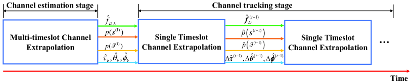
Figure 6: The flow chart of the proposed two-stage channel extrapolation scheme.

The received signal model (28) can be rewritten as a standard CS model

$$\mathbf{y}^{(t)} =\boldsymbol{\Phi}^{(t)}\boldsymbol{h}_{d}^{(t)}+\mathbf{n}^{(t)},$$ (34)

where $\boldsymbol{\Phi}^{(t)}=[\boldsymbol{A}_{R}\otimes(\textrm{diag}(\mathbf{x})\mathbf{W}^{(t)}\boldsymbol{\Lambda}^{(t)}\mathbf{S}^{(t)}\mathbf{F}_{d})]\mathbf{D}^{(t)}\in\mathbb{C}^{N_{r}P\times N_{r}L}$. At the $t$-th SRS symbol, we aim to track the time-varying DAD channel $\boldsymbol{h}_{d}^{(t)}$, the off-grid vector $\boldsymbol{\varDelta}^{(t)}$, and the imperfection parameter $\boldsymbol{\xi}^{(t)}\triangleq\{\boldsymbol{f}_{D}^{(t)},\varepsilon^{(t)},\tau_{0}^{(t)}\}$ based on the observations $\mathbf{y}^{(T)}$. In particular, given the imperfection parameters $\boldsymbol{\xi}^{(t)}$ and the off-grid vector $\boldsymbol{\varDelta}^{(t)}$, we are interested in computing the MMSE estimates of $\boldsymbol{h}_{d}^{(t)}$, i.e., $\hat{h}_{d,m}^{(t)}=\mathrm{\mathbf{E}}\left[h_{d,m}^{(t)}|\mathbf{y}^{(T)};\boldsymbol{\xi}^{(t)},\boldsymbol{\varDelta}^{(t)}\right],m=1,...,LN_{r}$, where the expectation is over the marginal posterior

$$p\left(h_{d,m}^{(t)}|\mathbf{y}^{(T)};\boldsymbol{\xi}^{(t)},\boldsymbol{\varDelta}^{(t)}\right)\propto$$

$$\thinspace\thinspace\thinspace\thinspace\sum_{\boldsymbol{s}^{(T)}}\int_{-h_{d,m}^{(t)},\boldsymbol{\vartheta}^{(T)}}p\left(\mathbf{y}^{(T)},\boldsymbol{v}^{(T)};\boldsymbol{\xi}^{(t)},\boldsymbol{\varDelta}^{(t)}\right),$$ (35)

where $\boldsymbol{v}^{(T)}$ denotes collections $\{\boldsymbol{v}^{(t)}\}_{t=1}^{T}$ with $\boldsymbol{v}^{(t)}\triangleq[\boldsymbol{h}_{d}^{(t)},\boldsymbol{\vartheta}^{(t)},\boldsymbol{s}^{(t)}]$, $\int_{-h_{d,m}^{(t)}}$ denotes the vector collections integration over $\boldsymbol{h}_{d}^{(T)}$ excluding the element $h_{d,m}^{(t)}$. It is difficult to calculate the exact posterior in (35) because the corresponding factor graph has loops. Consequently, we propose an efficient tracking algorithm combining the sum-product message-passing (SPMP) algorithm [29] and the turbo framework [30] to calculate an approximate marginal posterior of $p(h_{d,m}^{(t)}|\mathbf{y}^{(T)};\boldsymbol{\xi}^{(t)},\boldsymbol{\varDelta}^{(t)})$.

Besides, the imperfection parameters $\boldsymbol{\xi}^{(t)}$ and the off-grid parameters $\boldsymbol{\varDelta}^{(t)}$ at time $t$ can be obtained by the maximum a posterior (MAP) estimator as follows:

$$\hat{\boldsymbol{\Xi}}^{(t)} =\mathrm{arg}\max_{\boldsymbol{\Xi}^{(t)}}\ln p\left(\boldsymbol{\Xi}^{(t)}|\mathbf{y}^{(T)}\right)$$

$$\propto\mathrm{arg}\max_{\boldsymbol{\Xi}^{(t)}}\ln\int p\left(\boldsymbol{h}_{d}^{(T)},\mathbf{y}^{(T)},\boldsymbol{\Xi}^{(t)}\right)d\boldsymbol{h}_{d}^{(T)},$$ (36)

where $\boldsymbol{\Xi}^{(t)}\triangleq\{\boldsymbol{\xi}^{(t)},\boldsymbol{\varDelta}^{(t)}\}$. It is a high-dimensional non-convex objective function and we cannot obtain a closed-form expression due to the multi-dimensional integration over $\boldsymbol{h}_{d}^{(T)}$. To handle this issue, we adopt majorization-minimization (MM) method to construct a surrogate function and then use AO method to find a stationary point of (36). Inspired by the EM method [31], the channel tracking algorithm performs iterations between following two steps until convergence at each time $t$.

• DAD Channel Estimation (E-step): Given $\boldsymbol{\Xi}^{(t)}$, calculate the approximate posterior $\hat{p}\left(h_{d,m}^{(t)}|\mathbf{y}^{(T)};\boldsymbol{\Xi}^{(t)}\right)$ via the dynamic Turbo framework, as elaborated in Subsection IV-D.

• Off-grid and Imperfection Parameters Estimation (M-step): Given the estimate of $\boldsymbol{\Xi}^{(t-1)}$ from the previous time $t-1$, $\hat{p}(\boldsymbol{h}_{d}^{(t)}|\mathbf{y}^{(T)};\boldsymbol{\Xi}^{(t)})$ from the E-Step, construct surrogate functions for the MAP objective function in (36), then maximize the surrogate function with respect to $\boldsymbol{\Xi}^{(t)}$, as elaborated in Subsection IV-E.

IV-D E-Step

At the $t$-th SRS symbol, the E-Step contains two modules based on the Turbo-CS framework as shown in Fig. 7: Module A is a linear minimum mean square error (LMMSE) estimator based on the current observation $\mathbf{y}^{(t)}$ and messages from Module B, while Module B is a sparsity combiner performing MMSE estimation that combines the channel prior passed from the previous timeslot and the messages from Module A. The two modules are executed iteratively until convergence.

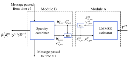
Figure 7: An illustration of the Turbo-CS framework.

IV-D1 Module A

In Module A, the DAD channel vector $\boldsymbol{h}_{d}^{(t)}$ is estimated based on the current observation $\mathbf{y}^{(t)}$ and a prior distribution $\mathcal{CN}(\boldsymbol{h}_{d}^{(t)};\boldsymbol{h}_{A,pri}^{(t)},\textrm{diag}(\boldsymbol{v}_{A,pri}^{(t)}))$, where $\boldsymbol{h}_{A,pri}^{(t)}$ and $\boldsymbol{v}_{A,pri}^{(t)}$ are the extrinsic message output from Module B. Then, the LMMSE estimate of $\boldsymbol{h}_{d}^{(t)}$ still follows a complex Gaussian distribution with mean and variance given by

$$\boldsymbol{V}_{A,post}^{\left(t\right)}=\left((\boldsymbol{\Phi}^{(t)\thinspace H}\boldsymbol{\Phi}^{(t)})/(\sigma_{e}^{(t)})^{2}+\textrm{diag}(1/\boldsymbol{v}_{A,pri}^{(t)})\right)^{-1},$$ (37)

$$\boldsymbol{h}_{A,post}^{\left(t\right)}=\boldsymbol{V}_{A,post}^{\left(t\right)}\left(\frac{\boldsymbol{h}_{A,pri}^{(t)}}{\boldsymbol{v}_{A,pri}^{(t)}}+\frac{\boldsymbol{\Phi}^{(t)H}\mathbf{y}^{(t)}}{(\sigma_{e}^{(t)})^{2}}\right).$$

Then, the extrinsic message passed to Module B can be calculated as [30]

$$\boldsymbol{h}_{B,pri}^{\left(t\right)}=\boldsymbol{v}_{B,pri}^{\left(t\right)}\left(\boldsymbol{h}_{A,post}^{\left(t\right)}/\boldsymbol{v}_{A,post}^{\left(t\right)}-\boldsymbol{h}_{A,pri}^{\left(t\right)}/\boldsymbol{v}_{A,pri}^{\left(t\right)}\right),$$ (38)

$$\boldsymbol{v}_{B,pri}^{\left(t\right)}=\left(1/\boldsymbol{v}_{A,post}^{\left(t\right)}-1/\boldsymbol{v}_{A,pri}^{\left(t\right)}\right)^{-1}.$$

IV-D2 Module B

We assume that $\boldsymbol{h}_{B,pri}^{(t)}$ is modeled as an AWGN observation [30, 27]:

$$\boldsymbol{h}_{B,pri}^{(t)}=\boldsymbol{h}_{d}^{(t)}+\mathbf{z}^{(t)},$$ (39)

where $\mathbf{z}^{(t)}\sim\mathcal{CN}(0,\textrm{diag}(\boldsymbol{v}_{B,pri}^{(t)}))$ is independent of $\boldsymbol{h}_{d}^{(t)}$. Under this assumption, the factor graph (denoted as $\mathcal{F}$) of the joint probability distribution $p(\boldsymbol{h}_{d}^{(T)},$$\boldsymbol{s}^{(T)},$$\boldsymbol{\vartheta}^{(T)},$$\boldsymbol{h}_{B,pri}^{(T)};$$\boldsymbol{\xi}^{\left(t\right)},$$\boldsymbol{\varDelta}^{(t)})$ is shown in Fig. 8, where the function expression of each factor node is listed in Table I. Based on (39), we combine the dynamic sparsity prior information of $\boldsymbol{h}_{d}^{(t)}$ and the extrinsic messages from Module A to calculate the posterior distributions $p(h_{d,m}^{(t)}\mid\boldsymbol{h}_{B,pri}^{(t)})$ by performing SPMP over the factor graph $\mathcal{F}$. We now outline the message passing procedure.

Figure 8: An illustration of factor graph $\mathcal{F}$.

TABLE I: Factors and distributions forms in Fig. 8.

Factor	Distribution
$d_{m}^{(t)}(s_{m}^{(t)},s_{m}^{(t-1)})$	$\!\!\!\begin{array}[]{l}\!\!p\left(s_{m}^{(t)}|s_{m}^{(t-1)}\right)\!\\ =\begin{cases}\!\left(\rho_{10}\right)^{1-s_{m}^{(t)}}\!\left(1\!-\!\rho_{10}\right)^{s_{m}^{(t)}}&\!\!\!\!s_{m}^{(t-1)}\!=\!1\\ \!\left(\rho_{01}\right)^{s_{m}^{(t)}}\!\left(1\!-\!\rho_{01}\right)^{1-s_{m}^{(t)}}&\!\!\!\!s_{m}^{(t-1)}\!=\!0\end{cases}\end{array}$
$\begin{array}[]{c}x_{m}^{(t)}(\vartheta_{m}^{(t)},\vartheta_{m}^{(t-1)})\end{array}$	$\begin{array}[]{l}\!\!p\left(\vartheta_{m}^{\left(t\right)}|\vartheta_{m}^{\left(t-1\right)}\right)=\\ \mathcal{CN}\!\!\left(\vartheta_{m}^{\left(t\right)};\!\left(1\!-\beta_{\vartheta}\right)\vartheta_{m}^{\left(t-1\right)}\!+\!\beta_{\vartheta}\mu_{\vartheta},\beta_{\vartheta}^{2}\gamma_{\vartheta}\!\right)\end{array}$
$f_{m}^{(t)}(\vartheta_{m}^{(t)},s_{m}^{(t)},h_{d,m}^{(t)})$	$\!\!\!\begin{array}[]{c}p\left(h_{d,m}^{\left(t\right)}|\vartheta_{m}^{\left(t\right)},s_{m}^{\left(t\right)}\right)=\delta\left(h_{d,m}^{\left(t\right)}-\vartheta_{m}^{\left(t\right)}s_{m}^{\left(t\right)}\right)\end{array}$
$g_{m}^{(t)}(h_{B,pri,m}^{(t)},h_{d,m}^{(t)})$	$p\left(h_{B,pri,m}^{\left(t\right)}|h_{d,m}^{\left(t\right)}\right)=\mathcal{CN}\left(h_{d,m}^{\left(t\right)};h_{B,pri,m}^{\left(t\right)},v_{B,pri,m}^{\left(t\right)}\right)$

At $\mathcal{F}_{t}$, the message from variable node $h_{d,m}^{\left(t\right)}$ to factor node $f_{m}^{\left(t\right)}$ is $\nu_{h_{d,m}^{(t)}\rightarrow f_{m}^{(t)}}(h_{d,m}^{(t)})=\mathcal{CN}(h_{d,m}^{(t)};h_{B,pri,m}^{(t)},v_{B,pri,m}^{(t)})$ and the message passing is performed over the path $x_{m}^{(t)}\rightarrow\vartheta_{m}^{(t)}\rightarrow f_{m}^{(t)}$ and $d_{m}^{(t)}\rightarrow s_{m}^{(t)}\rightarrow f_{m}^{(t)}$, respectively. Then, the marginal posterior distribution is given by

$$p\left(h_{d,m}^{(t)}|\boldsymbol{h}_{B,pri}^{\left(t\right)}\right)\!\propto\!\!\int_{\vartheta_{m}^{\left(t\right)}}\!\sum_{s_{m}^{(t)}}\!f_{m}^{(t)}\nu_{s_{m}^{(t)}\!\rightarrow f_{m}^{(t)}}\!\!\left(s_{m}^{(t)}\right)\nu_{\vartheta_{m}^{\left(t\right)}\!\rightarrow f_{m}^{(t)}}\!\!\left(\vartheta_{m}^{\left(t\right)}\right)$$

$$\thinspace\thinspace\thinspace\thinspace\thinspace\thinspace\thinspace\thinspace\thinspace\thinspace\thinspace\thinspace\thinspace\thinspace\thinspace\thinspace\thinspace\thinspace\thinspace\thinspace\thinspace\thinspace\thinspace\thinspace\thinspace\thinspace\thinspace\thinspace\thinspace\thinspace\thinspace\thinspace\thinspace\thinspace\thinspace\thinspace\thinspace\thinspace\thinspace\thinspace\thinspace\thinspace\thinspace\thinspace\times\nu_{h_{d,m}^{\left(t\right)}\!\rightarrow f_{m}^{(t)}}\!\!\left(h_{d,m}^{\left(t\right)}\right).$$ (40)

Finally, the extrinsic mean and variance are given by

$$\boldsymbol{h}_{A,pri}^{\left(t\right)}=\boldsymbol{v}_{A,pri}^{\left(t\right)}\left(\boldsymbol{h}_{B,post}^{\left(t\right)}/\boldsymbol{v}_{B,post}^{\left(t\right)}-\boldsymbol{h}_{B,pri}^{\left(t\right)}/\boldsymbol{v}_{B,pri}^{\left(t\right)}\right),$$

$$\begin{gathered}\boldsymbol{v}_{A,pri}^{\left(t\right)}=\left(1/\boldsymbol{v}_{B,post}^{\left(t\right)}-1/\boldsymbol{v}_{B,pri}^{\left(t\right)}\right)^{-1},\end{gathered}$$ (41)

where $\boldsymbol{h}_{B,post}^{(t)}$ and $\boldsymbol{v}_{B,post}^{(t)}$ denote the posterior mean and variance corresponding to $p(h_{d,m}^{(t)}|\boldsymbol{h}_{B,pri}^{(t)})$. After the convergence of the message passing over $\mathcal{F}_{t}$, the message passing is performed across time $\mathcal{F}_{t}\rightarrow\mathcal{F}_{t+1}$ over the path $f_{m}^{\left(t\right)}\rightarrow s_{m}^{(t)}\rightarrow d_{m}^{\left(t+1\right)}$ and $f_{m}^{\left(t\right)}\rightarrow\vartheta_{m}^{\left(t\right)}\rightarrow x_{m}^{\left(t+1\right)}$, and $\hat{p}(\boldsymbol{s}^{(t)})=\prod_{m=1}^{LN_{r}}\hat{p}(s_{m}^{(t)})$, $\hat{p}(\boldsymbol{\vartheta}^{(t)})=\prod_{m=1}^{LN_{r}}\hat{p}(\vartheta_{m}^{(t)})$, where

$$\hat{p}\left(s_{m}^{(t)}\right) \triangleq\nu_{s_{m}^{(t)}\rightarrow d_{m}^{\left(t+1\right)}}\left(s_{m}^{(t)}\right),$$ (42)

$$\hat{p}\left(\vartheta_{m}^{\left(t\right)}\right) \triangleq\nu_{\vartheta_{m}^{\left(t\right)}\rightarrow x_{m}^{\left(t+1\right)}}\left(\vartheta_{m}^{\left(t\right)}\right).$$

IV-E M-Step

In the M-Step, we construct a surrogate function at fixed point $\dot{\boldsymbol{\Xi}}^{(t)}$ for the objective function of the MAP problem in (36) based on the MM method as [32, 33] :

$$u(\boldsymbol{\Xi}^{(t)};\dot{\boldsymbol{\Xi}}^{(t)})\!\!=\!\!\int\!\!p(\boldsymbol{h}_{d}^{(t)}\!\mid\!\mathbf{y}^{(T)},\dot{\boldsymbol{\Xi}}^{(t)})\ln\frac{p(\boldsymbol{h}_{d}^{(t)}\!,\mathbf{y}^{(T)}\!,\boldsymbol{\Xi}^{(t)})}{p(\boldsymbol{h}_{d}^{(t)}\!\mid\!\mathbf{y}^{(T)},\dot{\boldsymbol{\Xi}}^{(t)})}d\boldsymbol{h}_{d}^{(t)},$$ (43)

which satisfies basic properties

$$u(\boldsymbol{\Xi}^{(t)};\dot{\boldsymbol{\Xi}}^{(t)})\leq\ln p(\boldsymbol{\Xi}^{(t)},\mathbf{y}^{(T)}),$$

$$u(\dot{\boldsymbol{\Xi}}^{(t)};\dot{\boldsymbol{\Xi}}^{(t)})=\ln p(\dot{\boldsymbol{\Xi}}^{(t)},\mathbf{y}^{(T)}),$$

$$\left.\frac{\partial u(\boldsymbol{\Xi}^{(t)};\dot{\boldsymbol{\Xi}}^{(t)})}{\partial\boldsymbol{\Xi}^{(t)}}\right|_{\boldsymbol{\Xi}^{(t)}=\dot{\boldsymbol{\Xi}}^{(t)}}=\left.\frac{\partial\ln p(\boldsymbol{\Xi}^{(t)},\mathbf{y}^{(T)})}{\partial\boldsymbol{\Xi}^{(t)}}\right|_{\boldsymbol{\Xi}^{(t)}=\dot{\boldsymbol{\Xi}}^{(t)}},$$

for $\forall\boldsymbol{\Xi}^{(t)}$. Then, we partition $\boldsymbol{\Xi}^{(t)}$ into $B=6$ blocks with $\Xi_{1}^{(t)}=\varepsilon^{(t)}$, $\Xi_{2}^{(t)}=\tau_{0}^{(t)}$, $\boldsymbol{\Xi}_{3}^{(t)}=\boldsymbol{f}_{D}^{(t)}$, $\boldsymbol{\Xi}_{4}^{(t)}=\Delta\boldsymbol{\tau}^{(t)}$, $\boldsymbol{\Xi}_{5}^{(t)}=\Delta\boldsymbol{\theta}^{(t)}$, $\boldsymbol{\Xi}_{6}^{(t)}=\Delta\boldsymbol{\phi}^{(t)}$ based on their distinct physical meaning, and alternatively update $\Xi_{b}^{(t)}$ for $b=1,...,B$ as

$$\boldsymbol{\Xi}_{b}^{(t)(j+1)} =\mathrm{arg}\max_{\boldsymbol{\Xi}_{b}^{(t)}}u(\boldsymbol{\Xi}_{b}^{(t)},\boldsymbol{\Xi}_{-b}^{(t)(j)};\boldsymbol{\Xi}_{b}^{(t)(j)},\boldsymbol{\Xi}_{-b}^{(t)(j)}),$$ (44)

where $\boldsymbol{\Xi}_{-b}^{(t)(j)}=(\boldsymbol{\Xi}_{1}^{(t)(j+1)},...,\boldsymbol{\Xi}_{b-1}^{(t)(j+1)},\boldsymbol{\Xi}_{b+1}^{(t)(j)},...,\boldsymbol{\Xi}_{B}^{(t)(j)})$, and $j$ stands for the $j$-th iteration. We can obtain a closed-form solution of (44) for $\varepsilon^{(t)}$ as $\hat{\varepsilon}^{(t)}$$=$$\angle((\boldsymbol{\Phi}^{(t)}\boldsymbol{\mu}_{d}^{(t)})^{H}\mathbf{y}^{(t)})$, where $\boldsymbol{\mu}_{d}^{(t)}$ is the posterior mean of $\hat{p}(\boldsymbol{h}_{d}^{(t)}|\mathbf{y}^{(T)};\boldsymbol{\Xi}^{(t)})$ estimated in the E-Step. However, the surrogate functions for other variables are non-convex and it is difficult to find their optimal solutions. Therefore, we use a fixed stepsize one-step gradient update as in [33], i.e.,

$$\boldsymbol{\Xi}_{b}^{(t)(j+1)}=\boldsymbol{\Xi}_{b}^{(t)(j)}+\frac{\gamma_{b}}{50}\cdot\textrm{sign}(\boldsymbol{\zeta}_{b}^{(j)}), b=1,...,B,$$ (45)

where $\gamma_{b}$ stands for the grid interval, $\boldsymbol{\zeta}_{b}^{(j)}$ denotes the gradient of the objective function (43) with respect to $\boldsymbol{\Xi}_{b}^{(t)}$, and sign(·) stands for the signum function. The convergence of this MM based algorithm to a stationary point is guaranteed [32, Theorem 1]. Our proposed tracking scheme exploits prior information in the M-Step, i.e., $\hat{\boldsymbol{f}}_{D}^{(t-1)},\hat{\boldsymbol{\Delta}}^{(t-1)}$, based on the probability model (32)-(33) and has been well initialized. Hence, a good solution can always be found while the original EM method may easily trap into “bad” local optimums.

Finally, the overall channel extrapolation scheme in tracking stage at time $t$ is summarized in Algorithm 2.

Algorithm 2 Channel extrapolation scheme in tracking stage

Input: $\mathbf{Y}^{(t)},\hat{\boldsymbol{f}}_{D}^{(t-1)},\hat{\boldsymbol{\Delta}}^{(t-1)}$, EM iteration number $I_{EM}$.

Output: The recovered full-band CFR $\hat{\mathbf{H}}^{(t)}$, $\boldsymbol{\hat{\xi}}^{(t)},\hat{\boldsymbol{\Delta}}^{(t)}$.

1:  Initialization: $\boldsymbol{\hat{f}}_{D}^{(t)}=\boldsymbol{\hat{f}}_{D}^{(t-1)},\boldsymbol{\hat{\Delta}}^{(t)}=\boldsymbol{\hat{\Delta}}^{(t-1)}$.

2:  for ${\color[rgb]{0,0,1}{\color[rgb]{0,0,0}j=1,\cdots,I_{EM}}}$ do

3:     E-Step:

4:     while not converge do

5:        %Module A: LMMSE Estimator

6:        Calculate $\boldsymbol{V}_{A,post}^{(t)},\boldsymbol{h}_{A,post}^{(t)},\boldsymbol{h}_{B,pri}^{(t)},\boldsymbol{v}_{B,pri}^{(t)}$ in (37)-(38).

7:        %Module B: Sparsity Combiner

8:        Perform message passing over graph $\mathcal{F}_{t}$.

9:        Calculate $p(h_{d,m}^{(t)}|\boldsymbol{h}_{B,pri}^{(t)})$ in (40).

10:        Update $\boldsymbol{h}_{A,pri}^{(t)}$ and $\boldsymbol{v}_{A,pri}^{(t)}$in (41).

11:     end while

12:     M-Step

13:     Construct surrogate function in (43).

14:     Update $\boldsymbol{\Xi}_{b}^{(t)(j+1)},\forall b,$ in (44).

15:  end for

16:  Perform message passing $\mathcal{F}_{t}\rightarrow\mathcal{F}_{t+1}$.

17:  Calculate the recovered full-band CFR $\hat{\mathbf{H}}^{(t)}$ based on the estimated results $\hat{p}(\boldsymbol{h}_{d}^{(t)}|\mathbf{y}^{(T)})$ and $\hat{\boldsymbol{\Xi}}^{(t)}$.

18:  Pass the estimate $\hat{\boldsymbol{f}}_{D}^{(t)},\hat{\boldsymbol{\Delta}}^{(t)}$, and $\hat{p}(\boldsymbol{s}^{(t)})$, $\hat{p}(\boldsymbol{\vartheta}^{(t)})$ to the next time $\left(t+1\right)$.

IV-F Computational Complexity Analysis

The computational complexity of the channel tracking scheme in E-Step is dominated by the inverse operation in (37), which is $\mathcal{O}\left(N_{r}^{3}L^{3}\right)$, matrix multiplication in (37) to calculate $\boldsymbol{V}_{A,post}^{\left(t\right)}$ and $\boldsymbol{h}_{A,post}^{\left(t\right)}$, which is $\mathcal{O}\left(N_{r}^{3}L^{2}P\right)$ and $\mathcal{O}\left(N_{r}^{2}LP\right)$. Besides, the main computational complexity in M-Step is $\mathcal{O}\left(N_{r}^{3}L^{2}P\right)$ per iteration. Note that $L$ can be small in our problem since we adopt the off-grid adjustment strategy, which do not require a dense grid to guarantee the delay estimation accuracy.

V Simulation Results

In this section, we provide numerical results to evaluate the channel estimation performance of the proposed scheme. The MIMO-OFDM system is equipped with carrier frequency 3.5 GHz, the bandwidth $B$ = 60 MHz, and the subcarrier spacing $f_{s}=60$ KHz. The BS is equipped with $N_{r}=64$ ($N_{x}=N_{y}=8$) antennas and the user moves with speed 3 km/h. The bandwidth of each BWP is 30 MHz (15 MHz) and the number of the SRS sequence is $P=250$ (125) for $h_{p}=2$ (4). The $\textrm{SNR}=15$ dB and the delay grid size $L=26$. The CFR samples are generated by the QuaDRiGa toolbox [34] according to the 3D-UMa NLOS model defined by 3GPP R16 specifications [35] and the performance result of the algorithms is averaged over 500 noise realizations. We choose normalized mean square error (NMSE) as the performance metric to evaluate the extrapolation performance of various algorithms, which is defined as $\textrm{NMSE}=\frac{\left\|\hat{\mathbf{H}}^{(t)}-\mathbf{H}^{(t)}\right\|_{F}^{2}}{\left\|\mathbf{H}^{(t)}\right\|_{F}^{2}}$.

For comparison, we consider the following three benchmark schemes and use the same hopping SRSs pattern for all schemes for fairness.

• Baseline 1 : We employ the TST-MUSIC algorithm to perform channel extrapolation at each timeslot independently [19].

• Baseline 2 : We employ the OAMP based channel tracking algorithm to perform channel extrapolation [27]. Specifically, the channel tracking is performed at each BWP independently without frequency extrapolation and the BWP owning received SRSs can be estimated. Then, to achieve full-band channel estimation, a simple extrapolation in time-domain is employed: For each BWP, the rest channel (i.e., the white parts of channel in Fig. 9) estimation is seen as equivalent to the channel estimation results at the latest time, e.g., as shown in Fig. 9, the channel estimation results at the blocks with the same linestyle are equal.

• Baseline 3 We employ the proposed algorithm but without performing imperfection factors compensation and off-grid update, i.e., using TST-MUSIC algorithm in the channel estimation stage and proposed tracking algorithm without M-Step in the channel tracking stage.

  

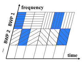
  Figure 9: An illustration of Baseline 2.

We first illustrate the convergence behavior of the proposed R-TST-MUSIC algorithm. As illustrated in Fig. 10, R-TST-MUSIC converges within 10 iterations (up to a small convergence error).

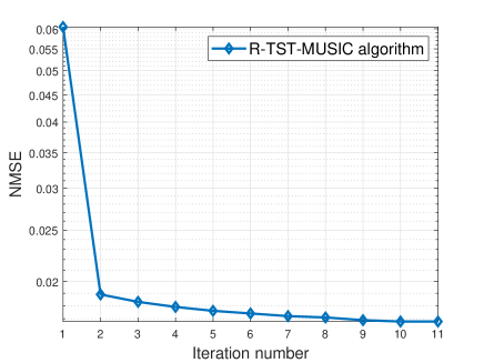
Figure 10: Convergence behavior of the R-TST-MUSIC algorithm.

In Fig. 11, we present the NMSE performance of the full-band channel versus time for various algorithms in both channel estimation and tracking stage. First, it can be seen that our proposed R-TST-MUSIC algorithm reaps a significant performance gain compared with original TST-MUSIC algorithm. Second, the extrapolation schemes (i.e., the proposed scheme and Baseline 3) achieve a better performance than the traditional channel tracking algorithm, i.e., Baseline 2. On one hand, it is mainly because Baseline 2 do not have a real extrapolation ability, i.e., without extrapolation in frequency domain, and the extrapolation in time domain has approximation error. Besides, since the channel for each BWP is estimated independently, it cannot fully exploit all observation information at different BWPs to improve the channel parameter estimation accuracy. On the other hand, as compared to Baseline 2, our proposed two-stage channel extrapolation scheme performs a meticulously designed multi-timeslot based channel estimation initially to provide a better initial value for doing channel tracking in the second stage. Finally, we observe that the proposed scheme outperforms Baseline 3 and TST-MUSIC algorithm, which demonstrates the necessity of the imperfection factors compensation and employing the off-grid channel model.

(a)

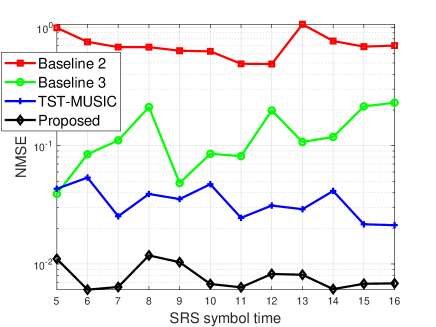
(b)

Figure 11: NMSE of the full-band channel versus time for $h_{p}=4$: (a) Channel estimation stage; (b) Channel tracking stage.

In Fig. 12, the NMSE performance of the first BWP channel is illustrated as a function of SRS symbol time. As can be seen, our proposed scheme outperforms other schemes for all times. Besides, the curves of Baseline 3 and the proposed scheme oscillate with the period $h_{p}$. It is reasonable since the position of SRSs in frequency domain undergoes periodic changes, and within a cycle, the first BWP becomes increasingly distant from the position of the SRSs in frequency domain as time increases, resulting in an increasing extrapolation distance. Furthermore, Baseline 3 exhibits the most intense oscillations, which indicates that the imperfection parameters will seriously affect the algorithm’s extrapolation ability if they are not well compensated for.

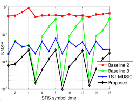
Figure 12: NMSE of the first BWP channel versus time for $h_{p}=4$.

Then, we investigate the extrapolation performance of our proposed scheme focusing on the $1+h_{p}n,n=0,...,N_{s}-1,$-th SRS symbol time, at all of which the SRSs locate in the first BWP. Fig. 13 depicts the NMSE performance of different BWPs for various SNRs with $h_{p}=4$, where the NMSE is averaged over $N_{s}=15$ SRS symbol times. It is observed that the NMSE increases with the BWP index due to the increased extrapolation range.

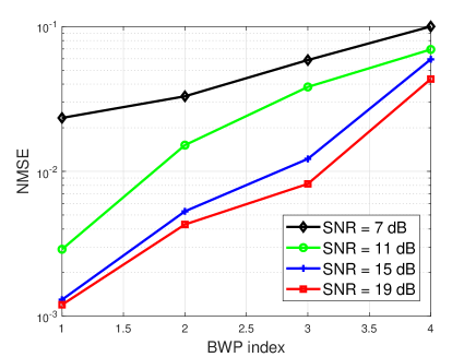
Figure 13: NMSE of different BWPs channel for $h_{p}=4$.

In Fig. 14, we investigate the time-averaged NMSE (TNMSE) performance versus SNR for $h_{p}=2$ and $h_{p}=4$, respectively, where $\textrm{TNMSE}=\frac{1}{T}\sum_{t=1}^{T}\frac{\left\|\hat{\mathbf{H}}^{(t)}-\mathbf{H}^{(t)}\right\|_{F}^{2}}{\left\|\mathbf{H}^{(t)}\right\|_{F}^{2}}$ with $T=60$. As can be seen, the TNMSE of all schemes decreases as SNR increases. Besides, our proposed scheme achieves significant performance gain compared with baselines for both $h_{p}=2$ and $h_{p}=4$. Furthermore, the algorithms have better performance in the case of $h_{p}=2$ than $h_{p}=4$ due to a relatively narrower extrapolation range.

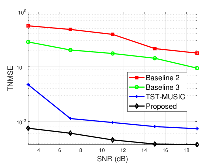
(a)

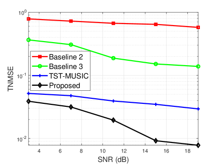
(b)

Figure 14: TNMSE versus SNR for: (a) $h_{p}=2$; (b) $h_{p}=4$.

VI Conclusion

In this paper, we proposed a two-stage 2D channel extrapolation scheme compatible with TDD massive MIMO 5G NR systems. We constructed a new received signal model for 2D channel extrapolation in the presence of imperfection factors based on a hopping pilot pattern. Then, in the channel estimation stage, we proposed a novel MBMT-HRPE scheme to compensate for the imperfection factors and achieve high-accuracy channel extrapolation. To avoid frequent multi-timeslot based channel estimation, we adopted a channel tracking scheme in the second stage. Finally, simulation results validated the effectiveness of our proposed channel extrapolation scheme.

References

- [1] E. G. Larsson, O. Edfors, F. Tufvesson, and T. L. Marzetta, “Massive MIMO for next generation wireless systems,” IEEE Commun. Mag., vol. 52, no. 2, pp. 186–195, 2014.
- [2] L. Lu, G. Y. Li, A. L. Swindlehurst, A. Ashikhmin, and R. Zhang, “An overview of massive MIMO: Benefits and challenges,” IEEE J. Select. Topics Signal Process., vol. 8, no. 5, pp. 742–758, 2014.
- [3] 3GPP, TS 38.211 V16.7.0 Release 16, Technical Specification Group Radio Access Network;NR;Physical channels and modulation, Sep. 2021.
- [4] A. Kalachikov and A. Stenin, “Performance evaluation of the SRS based MIMO channel estimation on 5G NR open source channel model,” in Proc. IEEE 22nd Int. Conf. Young Prof. Electron Devices Mater. (EDM). IEEE, 2021, pp. 124–127.
- [5] S. K. Sengijpta, “Fundamentals of statistical signal processing: Estimation theory,” 1995.
- [6] F. Rottenberg, T. Choi, P. Luo, C. J. Zhang, and A. F. Molisch, “Performance analysis of channel extrapolation in FDD massive MIMO systems,” IEEE Trans. Wireless Commun., vol. 19, no. 4, pp. 2728–2741, Apr. 2020.
- [7] M.-O. Pun, A. F. Molisch, P. Orlik, and A. Okazaki, “Super-resolution blind channel modeling,” in Proc. IEEE Int. Conf. Commun. (ICC), Jun. 2011, pp. 1–5.
- [8] N. Jalden, H. Asplund, and J. Medbo, “Channel extrapolation based on wideband MIMO measurements,” in Proc. 6th Eur. Conf. Antennas Propag. (EUCAP), Mar. 2012, pp. 442–446.
- [9] X. Xu, S. Zhang, F. Gao, and J. Wang, “Sparse Bayesian learning based channel extrapolation for RIS assisted MIMO-OFDM,” IEEE Trans. Commun., vol. 70, no. 8, pp. 5498–5513, Aug. 2022.
- [10] U. Ugurlu, R. Wichman, C. B. Ribeiro, and C. Wijting, “A multipath extraction-based CSI acquisition method for FDD cellular networks with massive antenna arrays,” IEEE Trans. Wireless Commun., vol. 15, no. 4, pp. 2940–2953, Apr. 2016.
- [11] M. Arnold, S. Dorner, S. Cammerer, J. Hoydis, and S. ten Brink, “Towards practical FDD massive MIMO: CSI extrapolation driven by deep learning and actual channel measurements,” in Proc. 53rd Asilomar Conf. Signals Syst. Comput., Nov. 2019, pp. 1972–1976.
- [12] Z. Zhong, L. Fan, and S. Ge, “FDD massive MIMO uplink and downlink channel reciprocity properties: Full or partial reciprocity?” in Proc. IEEE Global Commun. Conf. (GLOBECOM), Dec. 2020, pp. 1–5.
- [13] D. Vasisht, S. Kumar, H. Rahul, and D. Katabi, “Eliminating channel feedback in next-generation cellular networks,” in Proc. ACM SIGCOMM Conf., Aug. 2016, pp. 398–411.
- [14] R. O. Adeogun, P. D. Teal, and P. A. Dmochowski, “Extrapolation of MIMO mobile-to-mobile wireless channels using parametric-model-based prediction,” IEEE Trans. Veh. Technol., vol. 64, no. 10, pp. 4487–4498, Oct. 2015.
- [15] M. D. Larsen, A. L. Swindlehurst, and T. Svantesson, “Performance bounds for MIMO-OFDM channel estimation,” IEEE Trans. Signal Process., vol. 57, no. 5, pp. 1901–1916, May. 2009.
- [16] Y. Han, S. Jin, X. Li, C.-K. Wen, and T. Q. S. Quek, “Multi-domain channel extrapolation for FDD massive MIMO systems,” IEEE Trans. Commun., vol. 69, no. 12, pp. 8534–8550, Dec. 2021.
- [17] W. Guo, W. Zhang, P. Mu, F. Gao, and H. Lin, “High-mobility wideband massive MIMO communications: Doppler compensation, analysis and scaling laws,” IEEE Trans. Wireless Commun., vol. 18, no. 6, pp. 3177–3191, Jun. 2019.
- [18] H. Xu and L. Yang, “Calibration of random phase rotation for multi-band OFDM UWB signals,” in Proc. 44th Asilomar Conf. Signals Syst. Comput., Nov. 2010, pp. 170–174.
- [19] Y.-Y. Wang, J.-T. Chen, and W.-H. Fang, “TST-MUSIC for joint DOA-delay estimation,” IEEE Trans. Signal Process., vol. 49, no. 4, pp. 721–729, Apr. 2001.
- [20] X. Wu, X. Yang, S. Ma, B. Zhou, and G. Yang, “Hybrid channel estimation for UPA-assisted millimeter-wave massive MIMO IoT systems,” IEEE Internet Things J., vol. 9, no. 4, pp. 2829–2842, Feb. 2022.
- [21] K. Wong, Q.-T. Zhang, J. Reilly, and P. Yip, “On information theoretic criteria for determining the number of signals in high resolution array processing,” IEEE Trans. Acoust. Speech Signal Process., vol. 38, no. 11, pp. 1959–1971, Nov. 1990.
- [22] X. Li and K. Pahlavan, “Super-resolution TOA estimation with diversity for indoor geolocation,” IEEE Trans. Wireless Commun., vol. 3, no. 1, pp. 224–234, Jan. 2004.
- [23] D. P. Bertsekas, “Nonlinear programming,” Belmont, MA: Athena Scientific, 1995.
- [24] J. Ziniel and P. Schniter, “Dynamic compressive sensing of time-varying signals via approximate message passing,” IEEE Trans. Signal Process., vol. 61, no. 21, pp. 5270–5284, Nov. 2013.
- [25] J. Yu, X. Liu, Y. Gao, and X. Shen, “3D on and off-grid dynamic channel tracking for multiple UAVs and satellite communications,” IEEE Trans. Wireless Commun., vol. 21, no. 6, pp. 3587–3604, Jun. 2022.
- [26] X. Liu, W. Wang, X. Song, X. Gao, and G. Fettweis, “Sparse channel estimation via hierarchical hybrid message passing for massive MIMO-OFDM systems,” IEEE Trans. Wireless Commun., vol. 20, no. 11, pp. 7118–7134, Nov. 2021.
- [27] L. Lian, A. Liu, and V. K. Lau, “Exploiting dynamic sparsity for downlink FDD-massive MIMO channel tracking,” IEEE Trans. Signal Process., vol. 67, no. 8, pp. 2007–2021, 2019.
- [28] C. Zhang, D. Guo, and P. Fan, “Tracking angles of departure and arrival in a mobile millimeter wave channel,” in Proc. IEEE Int. Conf. Commun. (ICC), May. 2016, pp. 1–6.
- [29] F. Kschischang, B. Frey, and H.-A. Loeliger, “Factor graphs and the sum-product algorithm,” IEEE Trans. Inf. Theory, vol. 47, no. 2, pp. 498–519, Feb. 2001.
- [30] J. Ma, X. Yuan, and L. Ping, “Turbo compressed sensing with partial DFT sensing matrix,” IEEE Signal Process. Lett., vol. 22, no. 2, pp. 158–161, Feb. 2015.
- [31] C. LIU, Maximum likelihood estimation from incomplete data via em-type algorithms. Adv. Med. Statist., Nov. 2003.
- [32] A. Liu, G. Liu, L. Lian, V. K. N. Lau, and M.-J. Zhao, “Robust recovery of structured sparse signals with uncertain sensing matrix: A Turbo-VBI approach,” IEEE Trans. Wireless Commun., vol. 19, no. 5, pp. 3185–3198, May. 2020.
- [33] J. Dai, A. Liu, and V. K. N. Lau, “FDD massive MIMO channel estimation with arbitrary 2D-array geometry,” IEEE Trans. Signal Process., vol. 66, no. 10, pp. 2584–2599, May. 2018.
- [34] S. Jaeckel, L. Raschkowski, K. Borner, and L. Thiele, “Quadriga: A 3-D multi-cell channel model with time evolution for enabling virtual field trials,” IEEE Trans. Antennas Propag., vol. 62, no. 6, pp. 3242–3256, Jun. 2014.
- [35] 3GPP, “Study on channel model for frequencies from 0.5 to 100 GHz (3GPP TR 38.901 version 16.1.0 release 16),” Dec. 2019.