Designing Observables for Measurements
with Deep Learning

Abstract

Many analyses in particle and nuclear physics use simulations to infer fundamental, effective, or phenomenological parameters of the underlying physics models. When the inference is performed with unfolded cross sections, the observables are designed using physics intuition and heuristics. We propose to design optimal observables with machine learning. Unfolded, differential cross sections in a neural network output contain the most information about parameters of interest and can be well-measured by construction. We demonstrate this idea using two physics models for inclusive measurements in deep inelastic scattering.

1 Introduction

Simulations are widely used for parameter estimation in particle and nuclear physics. A typical analysis will follow one of two paths: forward-folding or unfolding. In the forward-folding pipeline, the target physics model must be specified at the time of inference. We focus on unfolding, where detector distortions are corrected in a first step (unfolding) and then the resulting cross section can be analyzed in the context of many models by any end users. In the unfolding pipeline, the first step is to identify observables sensitive to a given parameter(s). These are typically identified using physical reasoning. Then, the differential cross sections of these observables are measured, which includes unfolding with uncertainty quantification. Finally, the measured cross sections are fit to simulation templates with different values of the target parameters. This approach has been deployed to measure fundamental parameters like the top quark mass CMS:2022kqg and the strong coupling constant $\alpha_{s}(m_{Z})$ H1:2017bml ; Collaboration:2023xha as well as parton distribution functions H1:2015ubc ; Harland-Lang:2016yfn ; Hou:2019efy ; NNPDF:2021njg and effective or phenomenological parameters in parton shower Monte Carlo programs Campbell:2022qmc .

A key drawback of the standard pipeline is that the observables are constructed manually. There is no guarantee that the observables are maximally sensitive to the target parameters. Additionally, the observables are usually chosen based on particle-level information alone and so detector distortions may not be small. Such distortions can reduce the sensitivity to the target parameter once they are corrected for by unfolding. In some cases, the particle-level observable must be chosen manually because it must be calculable precisely in perturbation theory. There have been proposals to optimize the detector-level observable for a given particle-level observable Arratia:2022wny since they do not need to be the same. Alternatively, one could measure the full phase space and project out the desired observable after the fact Arratia:2021otl  Datta:2018mwd ; bunse2018unification ; Ruhe2019MiningFS ; Andreassen:2019cjw ; Bellagente:2019uyp ; 1800956 ; Vandegar:2020yvw ; Andreassen:2021zzk ; Howard:2021pos ; Backes:2022vmn ; Chan:2023tbf ; Shmakov:2023kjj ; Alghamdi:2023emm ; H1:2021wkz ; H1prelim-22-031 ; H1:2023fzk ; H1prelim-21-031 ; LHCb:2022rky ; Komiske:2022vxg ; Song:2023sxb . When the inference is directly based on Monte Carlo simulations, the particle-level observable is not fixed by perturbative calculability.

We propose to use machine learning for designing observables that are maximally sensitive to a given parameter(s) while also being minimally sensitive to detector distortions. Simultaneous optimization ensures that we only use regions of phase space that are measurable. A tailored loss function is used to train neural networks. We envision that this approach could be used for any case where simulations are used for parameter estimation. For concreteness, we demonstrate the new technique to the case of differentiating two parton shower Monte Carlo models of deep inelastic scattering. While neither model is expected to match data exactly, the availability of many events with corresponding detailed simulations makes this a useful benchmark problem. We do not focus on the parameter estimation step itself, but there are many proposals for doing this optimally with machine learning Brehmer:2018kdj ; Brehmer:2018eca ; Brehmer:2018hga ; DeCastro:2018psv ; Elwood:2018qsr ; Andreassen:2019nnm ; Brehmer:2019xox ; Wunsch:2020iuh ; Ghosh:2021roe ; GomezAmbrosio:2022mpm ; Simpson:2022suz .

This paper is organized as follows. Section 2 introduces our approach to observable construction. The datasets used for demonstrating the new method are introduced in Sec. 3. Results with these datasets are presented in Sec. 4. The paper ends with conclusions and outlook in Sec. 5.

2 Methodology

We begin by constructing new observables that are simultaneously sensitive to a parameter while also being minimally sensitive to detector effects. We introduce the method with a toy model for continuous parameter estimation, which demonstrates the essential ideas in a simplified context. This is followed by a more complete binary classification example using simulated deep inelastic scattering events from the H1 experiment at HERA, where the goal is to be maximally sensitive to distinguishing two datasets.

2.1 Toy example for continuous parameter estimation

For each event, we have pairs $(Z,X)$ where $Z$ represents the particle-level observable and $X$ represents the detector-level observable. Capital letters represent random variables while lower-case letter represent realizations of the corresponding random variables. We consider the case $X$ and $Z$ have the same structure, i.e. they are both sets of 4-vectors. This is the standard case where $X$ is a set of energy-flow objects that are meant to correspond to the 4-vectors of particles before being distorted by the detector. Furthermore, we fix the same definition of the observable at particle and detector level. The training samples are generated with a uniform distribution for the parameter of interest $\mu$, so each event is specified by $(\mu_{i},z_{i},x_{i})$. Then, we parameterize the observable $f$ as a neural network and optimize the following loss function:

$$L[f]=\sum_{i}(f(x_{i})-\mu_{i})^{2}+\lambda\sum_{i}(f(x_{i})-f(z_{i}))^{2}\,,$$ (1)

where the form of both terms is the usual mean squared error loss used in regression tasks. The first term trains the regression to predict the parameter of interest $\mu$ while the second term trains the network to make the predictions given detector level features $x$ and particle level features $z$ similar. The hyperparameter $\lambda$ must be tuned and controls the trade off between sensitivity to the parameter of interest $\mu$ and sensitivity to detector effects.

The loss function in Eq. 1 is similar to the setting of decorrelation, where a classifier is trained to be independent from a given feature Blance:2019ibf ; Englert:2018cfo ; Louppe:2016ylz ; Dolen:2016kst ; Moult:2017okx ; Stevens:2013dya ; Shimmin:2017mfk ; Bradshaw:2019ipy ; ATL-PHYS-PUB-2018-014 ; DiscoFever ; Wunsch:2019qbo ; Rogozhnikov:2014zea ; 10.1088/2632-2153/ab9023 ; Kasieczka:2020pil ; Kitouni:2020xgb ; Estrade:2019gzk ; Aguilar-Saavedra:2017rzt ; aguilarsaavedra2020mass . One could apply decorrelation techniques in this case to ensure the classifier is not able to distinguish between features at detector level and at particle level. However, this will only ensure that the probability density for $f$ is the same for particle level and detector level. To be well-measured, we need more than statistical similarity between distributions - we need them to be similar event by event. The final term in Eq. 1 is designed for exactly this purpose.

All deep neural networks are implemented in Keras chollet2015keras /TensorFlow tensorflow and optimized using Adam adam . The network models use two hidden layers with 50 nodes per layer and Rectified Linear Unit (ReLU) activation functions for intermediate layers and a linear activation function for the last layer.

Figure 1: Input features and resolution model for toy regression example. Two different experimental resolution functions, A and B, are shown.

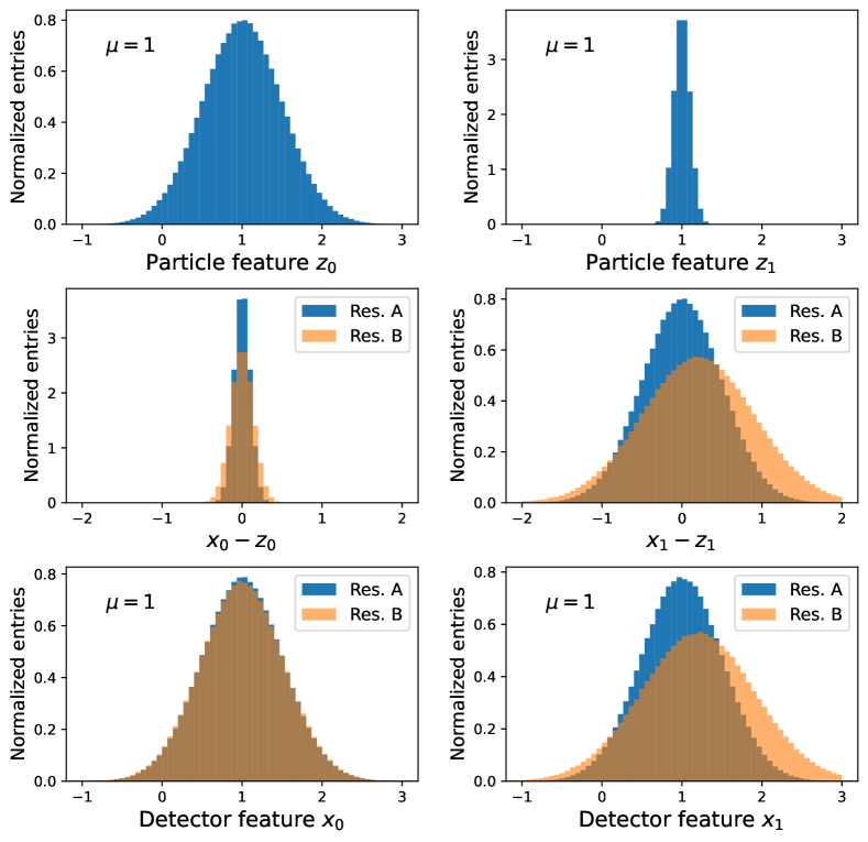
Figure 1 illustrates the input features and resolution model for the toy study. Two particle-level features $z_{0}$ and $z_{1}$ are modeled as normal distributions: $Z_{0}\sim\mathcal{N}(\mu,0.5)$ and $Z_{1}\sim\mathcal{N}(\mu,0.1)$, where feature 1 is significantly more sensitive to the parameter of interest $\mu$. The experimental resolution on the features is given by $X_{0}\sim\mathcal{N}(Z_{0},0.1)$ and $X_{1}\sim\mathcal{N}(Z_{1},0.5)$ so that feature 0 is well measured, while feature 1 has a relatively poor resolution. For this model, the net experimental sensitivity to $\mu$ is the same for both features, but feature 0 is much less sensitive to detector effects. Our proposed method will take this into account in the training of the neural network.

Figure 2: Results of toy regression example as a function of the $\lambda$ hyperparameter.

To demonstrate the sensitivity to uncertainties associated with detector effects, we make predictions using $f$ trained with resolution model A on a sample generated with resolution model B, shown in Figure 1, where the width is increased by a factor of 1.4 for both features and a bias of 0.2 is introduced for the $x_{1}$ feature. Figure 2 shows the results as a function of the $\lambda$ hyperparameter. With $\lambda=0$, which corresponds to the usual approach for this type of regression task, the correlation between each of the detector level features $x_{0}$ and $x_{1}$ and the network prediction $f$ is the same, reflecting the fact that $x_{0}$ and $x_{1}$ have the same sensitivity to $\mu$. As $\lambda$ increases, more emphasis is placed on feature $x_{0}$, which is well measured. The resolution of the regression, given by the RMS of $f$, starts at the expected value of about $\sqrt{0.5^{2}+0.1^{2}}/\sqrt{2}$ for resolution model A and $\lambda=0$ and increases with $\lambda$ as the network relies more on $x_{0}$ for the prediction. The bias in the prediction for resolution model B is large for $\lambda=0$ but falls significantly with increasing $\lambda$.

2.2 Full example for binary classification

In the binary case, we have two datasets generated from simulation 1 (sim. 1) and simulation 2 (sim. 2). The loss function for classification is given by

$$L[f]=-\sum_{i\in\text{sim. 1}}\log(f(z_{i}))-\sum_{i\in\text{sim. 2}}\log(1-f(z_{i}))+\lambda\sum_{i\in\text{sim. 1 \& 2}}(f(x_{i})-f(z_{i}))^{2}\,,$$ (2)

where the first two terms represent the usual binary cross entropy loss function for classification and the third term represents the usual mean squared error loss term for regression tasks. As in the regression case, the hyperparameter $\lambda$ must be tuned and controls the trade off between sensitivity to the dataset and sensitivity to detector effects. The network model is the same as in the previous example except that the final layer uses a sigmoid activation function. The binary case is a special case of the previous section where there are only two values of the parameter of interest. It may also be effective to train the binary case for a continuous parameter using two extreme values of the parameter. In this paper, we use high-quality, well-curated datasets from the binary case because of their availability, but it would be interesting to explore the continuous case in the future.

To determine the efficacy of the new observable, we unfold it with TUnfold version 17.9 Schmitt:2012kp through the interface included in the Root 6.24 Brun:1997pa distribution. The response matrix is defined from a 2D binning the NN output, given detector level and particle level features. The matrix uses 24 and 12 bins for detector and particle inputs, respectively, which gives reasonable stability and cross-bin correlations in the unfolding results. The ultimate test is to show that the difference between sim. 1 at detector-level unfolded with sim. 2 for the response matrix and the particle level sim. 1 (or vice versa) is smaller than the difference between sim. 1 and sim. 2 at particle level. In other words, this test shows that the ability to distinguish sim. 1 and sim. 2 significantly exceeds the modeling uncertainty from the unfolding.

3 Datasets

We use deep inelastic scattering events from high-energy electron-proton collisions to demonstrate the performance of the new approach. These simulated data are from the H1 experiment at HERA H1:1996jzy ; H1:1996prr and are used in the same way as Ref. Arratia:2021tsq . They are briefly described in the following.

Two parton shower Monte Carlo programs provide the particle-level simulation: Rapgap 3.1 Jung:1993gf or Djangoh 1.4 Charchula:1994kf . The energies of the incoming beams are $E_{e}=27.6$ GeV and $E_{p}=920$ GeV, for the lepton and proton, respectively, matching the running conditions of HERA II. Radiation from Quantum Electrodynamic processes is simulated by Heracles routines Spiesberger:237380 ; Kwiatkowski:1990cx ; Kwiatkowski:1990es in both cases. The outgoing particles from these two datasets are then fed into a Geant 3 geant4 -based detector simulation.

Following the detector simulation, events are reconstructed with an energy-flow algorithm energyflowthesis ; energyflowthesis2 ; energyflowthesis3 and the scattered electron is reconstructed using the default H1 approach H1:2012qti ; H1:2014cbm ; H1:2021wkz . Mis-measured backgrounds are suppressed with standard selections H1:2012qti ; H1:2014cbm . This whole process makes use of the modernized H1 computing environment at DESY Britzger:2021xcx . Each dataset is comprised of approximately 10 million events.

Figure 3: Particle level distributions of the nine NN input features for the Djangoh and Rapgap generators.

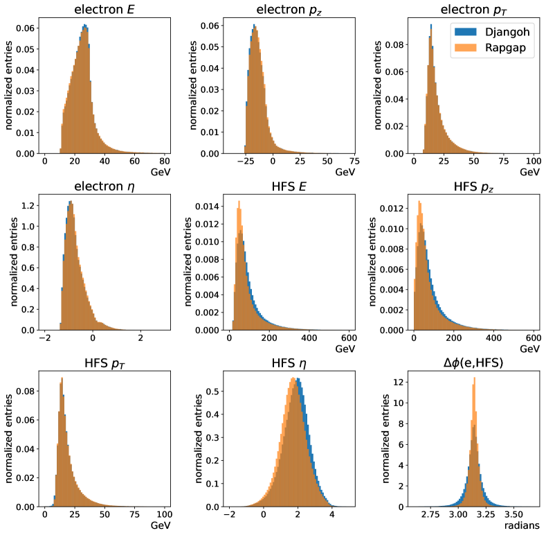
Figure 3 shows histograms of the nine features used as input for the neural network training. These features include the energy $E$, longitudinal momentum $p_{z}$, transverse momentum $p_{T}$, and pseudorapidity $\eta$ of the scattered electron and the total Hadronic Final State (HFS), as well as the difference in azimuthal angle between the two $\Delta\phi(e,{\rm HFS})$. The HFS is quite sensitive to the $\eta$ acceptance of the detector. In order to have HFS features that are comparable for the particle and detector definitions, we only use generated final state particles with $|\eta|<3.8$ in the definition of the particle-level HFS 4-vector. Both simulations provide event weights that must be used for physics analysis. In our study, we do not weight the simulated events in order to maximize the effective statistics of the samples in the neural network training. The electron feature distributions agree very well for the two simulations, while there are some visible differences in the HFS features.

4 Results

Figure 4: Neural Network output distributions for four values of the $\lambda$ hyperparameter, which sets the scale for the Detector - Particle disagreement penalty in the loss function. The top row shows the results for $\lambda=0$, where there is no penalty if the NN predictions for Detector-level input features and Particle-level input features disagree. The bottom three rows show increasing values of $\lambda$ : 1, 20, and 100.

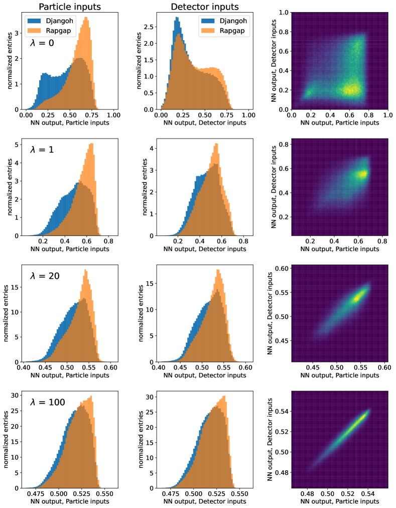
We now apply the method introduced in Sec. 2.2 to the DIS dataset described in Sec. 3. Figure 4 shows the results of four neural network trainings with different values of $\lambda$, which sets the relative weight of the MSE term in the loss function (Eq. 2) that controls the sensitivity to detector effects. With $\lambda=0$, the classification performance for particle-level inputs is strong, while there are significant disagreements between the particle and detector level neural network outputs. As $\lambda$ increases, the particle and detector level agreement improves at the cost of weaker classification performance. In what follows, we will use the network trained with $\lambda=100$. For a parameter estimation task, the entire distribution will be used for inference and therefore excellent event-by-event classification is not required.

Figure 5: Results of unfolding the NN output. The top (bottom) row shows the unfolding for the Rapgap (Djangoh) generator. The left column shows the response matrix for the unfolding, where the distribution of the NN output given the Detector-based input features (horizontal axis) is normalized to unit area for each bin of the NN output given the Particle-based input features (vertical axis). The center column shows the unfolded distribution compared to the true distribution. The right column shows the matrix of correlation coefficients from the unfolding.

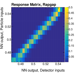
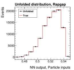
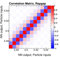
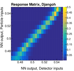
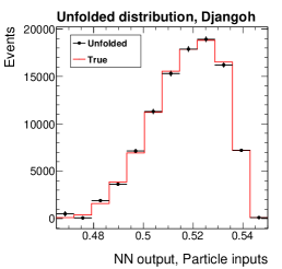
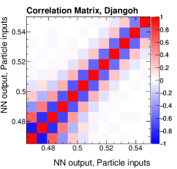
Next, we investigate how these spectra are preserved after unfolding. Figure 5 shows the results of unfolding the neural network output, given detector-level features, to give the neural network output distribution for particle-level features. The input distribution for the unfolding is $10^{5}$ events randomly chosen from a histogram of the neural network output for detector-level inputs from the simulation. The unfolding response matrices for the two simulations agree fairly well and are concentrated along the diagonal. The output of the unfolding shows very good agreement with the true distribution of the neural network output given particle-level inputs, demonstrating acceptable closure for the unfolding. The correlations in the unfolding result are mostly between neighboring bins of the distribution.

Figure 6: Results of testing the model dependence of the unfolding the neural network output distribution by varying the response matrix used in the unfolding. The top row normalizes the unfolded distribution with the true distribution from the same simulation, testing the unfolding closure (points) and unfolding model dependence (red histogram). The bottom row normalizes the unfolded distribution with the true distribution from the other simulation, showing the ability to distinguish the models.

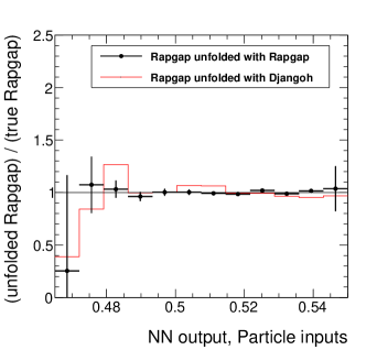
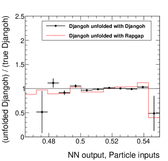
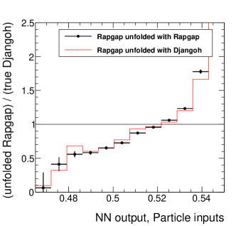
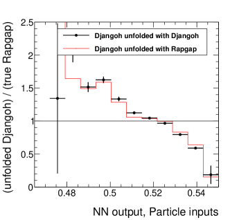
One of the biggest challenges for the $\lambda=0$ case is that it is highly sensitive to regions of phase space that are not well-constrained by the detector. As a result, the output of the unfolding is highly dependent on the simulation used in the unfolding (prior). Figure 6 shows the model dependence of the unfolding and the ability of the neural network to perform the model classification task. The top row of the figure shows the results of the closure tests compared with a measure of the unfolding model dependence, where we perform the unfolding with the response matrix from the other simulation. The unfolded distributions have been normalized using the true distribution from the same simulation, giving an expected flat distribution consistent with 1. The model dependence is small and generally less than 10%. The bottom row shows the unfolded distributions instead normalized by the true distribution from the other simulation. The degree to which the distribution deviates from unity is a measure of the model discrimination power of the network. The results show significant deviations from unity, indicating that the neural network can distinguish the two simulations. The size of the deviations from unity is large compared to the size of the model dependence of the unfolding.

Figure 7: Results of testing the model dependence of the unfolding the HFS $\eta$ distribution by varying the response matrix used in the unfolding. The top row normalizes the unfolded distribution with the true distribution from the same simulation, testing the unfolding closure (points) and unfolding model dependence (red histogram). The bottom row normalizes the unfolded distribution with the true distribution from the other simulation, showing the ability to distinguish the models.

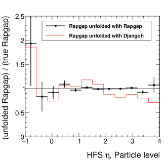
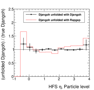
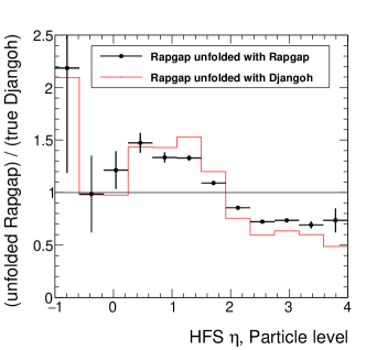
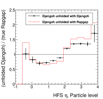
Figure 3 shows that some of the HFS variables in the input features may be able to distinguish the two models directly. Figure 7 shows the results of running the unfolding procedure using the HFS $\eta$ distribution for model discrimination, where the model dependence is significantly larger, compared to the neural network output. The shape is distorted, including deviations up to 20%, when the response matrix from the other simulation was used in the unfolding. Since the modeling uncertainty is comparable to or larger than the size of the effect we are trying to probe, such observables are much less useful than the neural network output for the inference task.

5 Conclusions and Outlook

Unfolded differential cross section measurements are a standard approach to making data available for downstream inference tasks. While some measurements can be used for a variety of tasks, often, there is a single goal that motivate the result. In these cases, we advocate to design observables that are tailored to the physics goal using machine learning. The output of a neural network trained specifically for the downstream task is an observable and its differential cross section likely contains more information than classical observables. We have proposed a new loss function for training the network so that the resulting observable can be well measured. We anticipate that our new approach could be useful for a variety of scientific goals, including measurements of fundamental parameters like the top quark mass and tuning Monte Carlo event generators.

There are a number of ways this approach could be extended in the future. We require that the observable have the same definition at particle level and detector level, while additional information at detector-level like resolutions may be useful to improve precision. A complementary strategy would be to use all the available information to unfold the full phase space Arratia:2021otl . Such techniques may improve the precision by integrating all of the relevant information at detector level, but they may compromise specific sensitivity by being broad and have no direct constraints on measurability. It would be interesting to compare our tailored approach to full phase space methods in the future.

Code availability

The code in this work can be found in: https://github.com/owen234/designer-obs-paper.

References

- (1) CMS Collaboration, A. Tumasyan, et al., Measurement of the differential production cross section as a function of the jet mass and extraction of the top quark mass in hadronic decays of boosted top quarks, Eur. Phys. J. C 83 (7) (2023) 560. arXiv:2211.01456, doi:10.1140/epjc/s10052-023-11587-8.
- (2) H1 Collaboration, V. Andreev, et al., Determination of the strong coupling constant in next-to-next-to-leading order QCD using H1 jet cross section measurements, Eur. Phys. J. C 77 (11) (2017) 791, [Erratum: Eur.Phys.J.C 81, 738 (2021)]. arXiv:1709.07251, doi:10.1140/epjc/s10052-017-5314-7.
- (3) ZEUS Collaboration, Z. Collaboration, Measurement of jet production in deep inelastic scattering and NNLO determination of the strong coupling at ZEUS (9 2023). arXiv:2309.02889.
- (4) H1, ZEUS Collaboration, H. Abramowicz, et al., Combination of measurements of inclusive deep inelastic scattering cross sections and QCD analysis of HERA data, Eur. Phys. J. C 75 (2015). arXiv:1506.06042, doi:10.1140/epjc/s10052-015-3710-4.
- (5) L. A. Harland-Lang, A. D. Martin, P. Motylinski, R. S. Thorne, The impact of the final HERA combined data on PDFs obtained from a global fit, Eur. Phys. J. C 76 (4) (2016) 186. arXiv:1601.03413, doi:10.1140/epjc/s10052-016-4020-1.
- (6) T.-J. Hou, et al., New CTEQ global analysis of quantum chromodynamics with high-precision data from the LHC, Phys. Rev. D 103 (1) (2021) 014013. arXiv:1912.10053, doi:10.1103/PhysRevD.103.014013.
- (7) NNPDF Collaboration, R. D. Ball, et al., The path to proton structure at 1% accuracy, Eur. Phys. J. C 82 (5) (2022) 428. arXiv:2109.02653, doi:10.1140/epjc/s10052-022-10328-7.
- (8) J. M. Campbell, et al., Event Generators for High-Energy Physics Experiments, in: Snowmass 2021, 2022. arXiv:2203.11110.
- (9) M. Arratia, D. Britzger, O. Long, B. Nachman, Optimizing observables with machine learning for better unfolding, JINST 17 (07) (2022) P07009. arXiv:2203.16722, doi:10.1088/1748-0221/17/07/P07009.
- (10) M. Arratia, et al., Publishing unbinned differential cross section results, JINST 17 (01) (2022) P01024. arXiv:2109.13243, doi:10.1088/1748-0221/17/01/P01024.
- (11) K. Datta, D. Kar, D. Roy, Unfolding with Generative Adversarial Networks (2018). arXiv:1806.00433.
- (12) M. Bunse, N. Piatkowski, T. Ruhe, W. Rhode, K. Morik, Unification of deconvolution algorithms for Cherenkov astronomy, in: 5th International Conference on Data Science and Advanced Analytics (DSAA), IEEE, 2018, pp. 21–30.
- (13) T. Ruhe, T. Voigt, M. Wornowizki, M. Börner, W. Rhode, K. Morik, Mining for spectra - the dortmund spectrum estimation algorithm, 2019.
- (14) A. Andreassen, P. T. Komiske, E. M. Metodiev, B. Nachman, J. Thaler, OmniFold: A Method to Simultaneously Unfold All Observables, Phys. Rev. Lett. 124 (2020) 182001. arXiv:1911.09107, doi:10.1103/PhysRevLett.124.182001.
- (15) M. Bellagente, A. Butter, G. Kasieczka, T. Plehn, R. Winterhalder, How to GAN away Detector Effects (2019). arXiv:1912.00477, doi:10.21468/SciPostPhys.8.4.070.
- (16) M. Bellagente, A. Butter, G. Kasieczka, T. Plehn, A. Rousselot, R. Winterhalder, Invertible Networks or Partons to Detector and Back Again (Jun 2020). arXiv:2006.06685, doi:10.21468/SciPostPhys.9.5.074.
-
(17)
M. Vandegar, M. Kagan, A. Wehenkel, G. Louppe,
Neural Empirical
Bayes: Source Distribution Estimation and its Applications to
Simulation-Based Inference, in: A. Banerjee, K. Fukumizu (Eds.),
Proceedings of The 24th International Conference on Artificial Intelligence
and Statistics, Vol. 130 of Proceedings of Machine Learning Research, PMLR,
2021, pp. 2107–2115.
arXiv:2011.05836.
URL https://proceedings.mlr.press/v130/vandegar21a.html - (18) A. Andreassen, P. T. Komiske, E. M. Metodiev, B. Nachman, A. Suresh, J. Thaler, Scaffolding Simulations with Deep Learning for High-dimensional Deconvolution, in: 9th International Conference on Learning Representations, 2021. arXiv:2105.04448.
- (19) J. N. Howard, S. Mandt, D. Whiteson, Y. Yang, Foundations of a Fast, Data-Driven, Machine-Learned Simulator (Jan 2021). arXiv:2101.08944.
- (20) M. Backes, A. Butter, M. Dunford, B. Malaescu, An unfolding method based on conditional Invertible Neural Networks (cINN) using iterative training (12 2022). arXiv:2212.08674.
- (21) J. Chan, B. Nachman, Unbinned profiled unfolding, Phys. Rev. D 108 (1) (2023) 016002. arXiv:2302.05390, doi:10.1103/PhysRevD.108.016002.
- (22) A. Shmakov, K. Greif, M. Fenton, A. Ghosh, P. Baldi, D. Whiteson, End-To-End Latent Variational Diffusion Models for Inverse Problems in High Energy Physics (5 2023). arXiv:2305.10399.
- (23) T. Alghamdi, et al., Toward a generative modeling analysis of CLAS exclusive photoproduction (7 2023). arXiv:2307.04450.
- (24) H1 Collaboration, V. Andreev, et al., Measurement of lepton-jet correlation in deep-inelastic scattering with the H1 detector using machine learning for unfolding (Aug 2021). arXiv:2108.12376.
(25)
H1 Collaboration,
Machine
learning-assisted measurement of multi-differential lepton-jet correlations
in deep-inelastic scattering with the H1 detector, H1prelim-22-031 (2022).
URL https://www-h1.desy.de/h1/www/publications/htmlsplit/H1prelim-22-031.long.html - (26) H1 Collaboration, V. Andreev, et al., Unbinned Deep Learning Jet Substructure Measurement in High ep collisions at HERA (3 2023). arXiv:2303.13620.
(27)
Measurement
of lepton-jet correlations in high neutral-current DIS with the H1
detector at HERA, H1prelim-21-031 (2021).
URL https://www-h1.desy.de/h1/www/publications/htmlsplit/H1prelim-21-031.long.html - (28) LHCb Collaboration, Multidifferential study of identified charged hadron distributions in -tagged jets in proton-proton collisions at 13 TeV (8 2022). arXiv:2208.11691.
- (29) P. T. Komiske, S. Kryhin, J. Thaler, Disentangling quarks and gluons in CMS open data, Phys. Rev. D 106 (9) (2022) 094021. arXiv:2205.04459, doi:10.1103/PhysRevD.106.094021.
- (30) STAR Collaboration, Y. Song, Measurement of CollinearDrop jet mass and its correlation with SoftDrop groomed jet substructure observables in GeV collisions by STAR (7 2023). arXiv:2307.07718.
- (31) J. Brehmer, K. Cranmer, G. Louppe, J. Pavez, Constraining Effective Field Theories with Machine Learning, Phys. Rev. Lett. 121 (11) (2018) 111801. arXiv:1805.00013, doi:10.1103/PhysRevLett.121.111801.
- (32) J. Brehmer, K. Cranmer, G. Louppe, J. Pavez, A Guide to Constraining Effective Field Theories with Machine Learning, Phys. Rev. D 98 (5) (2018) 052004. arXiv:1805.00020, doi:10.1103/PhysRevD.98.052004.
- (33) J. Brehmer, G. Louppe, J. Pavez, K. Cranmer, Mining gold from implicit models to improve likelihood-free inference, Proc. Nat. Acad. Sci. 117 (10) (2020) 5242–5249. arXiv:1805.12244, doi:10.1073/pnas.1915980117.
- (34) P. De Castro, T. Dorigo, INFERNO: Inference-Aware Neural Optimisation, Comput. Phys. Commun. 244 (2019) 170–179. arXiv:1806.04743, doi:10.1016/j.cpc.2019.06.007.
- (35) A. Elwood, D. Krücker, Direct optimisation of the discovery significance when training neural networks to search for new physics in particle colliders (6 2018). arXiv:1806.00322.
- (36) A. Andreassen, B. Nachman, Neural Networks for Full Phase-space Reweighting and Parameter Tuning, Phys. Rev. D 101 (9) (2020) 091901. arXiv:1907.08209, doi:10.1103/PhysRevD.101.091901.
- (37) J. Brehmer, F. Kling, I. Espejo, K. Cranmer, MadMiner: Machine learning-based inference for particle physics, Comput. Softw. Big Sci. 4 (1) (2020) 3. arXiv:1907.10621, doi:10.1007/s41781-020-0035-2.
- (38) S. Wunsch, S. Jörger, R. Wolf, G. Quast, Optimal Statistical Inference in the Presence of Systematic Uncertainties Using Neural Network Optimization Based on Binned Poisson Likelihoods with Nuisance Parameters, Comput. Softw. Big Sci. 5 (1) (2021) 4. arXiv:2003.07186, doi:10.1007/s41781-020-00049-5.
- (39) A. Ghosh, B. Nachman, D. Whiteson, Uncertainty-aware machine learning for high energy physics, Phys. Rev. D 104 (5) (2021) 056026. arXiv:2105.08742, doi:10.1103/PhysRevD.104.056026.
- (40) R. Gomez Ambrosio, J. ter Hoeve, M. Madigan, J. Rojo, V. Sanz, Unbinned multivariate observables for global SMEFT analyses from machine learning, JHEP 03 (2023) 033. arXiv:2211.02058, doi:10.1007/JHEP03(2023)033.
- (41) N. Simpson, L. Heinrich, neos: End-to-End-Optimised Summary Statistics for High Energy Physics, J. Phys. Conf. Ser. 2438 (1) (2023) 012105. arXiv:2203.05570, doi:10.1088/1742-6596/2438/1/012105.
- (42) A. Blance, M. Spannowsky, P. Waite, Adversarially-trained autoencoders for robust unsupervised new physics searches, JHEP 10 (2019) 047. arXiv:1905.10384, doi:10.1007/JHEP10(2019)047.
- (43) C. Englert, P. Galler, P. Harris, M. Spannowsky, Machine Learning Uncertainties with Adversarial Neural Networks, Eur. Phys. J. C79 (1) (2019) 4. arXiv:1807.08763, doi:10.1140/epjc/s10052-018-6511-8.
(44)
G. Louppe, M. Kagan, K. Cranmer,
Learning
to Pivot with Adversarial Networks, in: I. Guyon, U. V. Luxburg, S. Bengio,
H. Wallach, R. Fergus, S. Vishwanathan, R. Garnett (Eds.), Advances in
Neural Information Processing Systems, Vol. 30, Curran Associates, Inc.,
2017.
arXiv:1611.01046.
URL https://papers.nips.cc/paper/2017/hash/48ab2f9b45957ab574cf005eb8a76760-Abstract.html - (45) J. Dolen, P. Harris, S. Marzani, S. Rappoccio, N. Tran, Thinking outside the ROCs: Designing Decorrelated Taggers (DDT) for jet substructure, JHEP 05 (2016) 156. arXiv:1603.00027, doi:10.1007/JHEP05(2016)156.
- (46) I. Moult, B. Nachman, D. Neill, Convolved Substructure: Analytically Decorrelating Jet Substructure Observables (2017). arXiv:1710.06859.
- (47) J. Stevens, M. Williams, uBoost: A boosting method for producing uniform selection efficiencies from multivariate classifiers, JINST 8 (2013) P12013. arXiv:1305.7248, doi:10.1088/1748-0221/8/12/P12013.
- (48) C. Shimmin, P. Sadowski, P. Baldi, E. Weik, D. Whiteson, E. Goul, A. Sogaard, Decorrelated Jet Substructure Tagging using Adversarial Neural Networks, Phys. Rev. D96 (7) (2017) 074034. arXiv:1703.03507, doi:10.1103/PhysRevD.96.074034.
- (49) L. Bradshaw, R. K. Mishra, A. Mitridate, B. Ostdiek, Mass Agnostic Jet Taggers (2019). arXiv:1908.08959, doi:10.21468/SciPostPhys.8.1.011.
(50)
Performance of mass-decorrelated jet
substructure observables for hadronic two-body decay tagging in ATLAS,
Tech. Rep. ATL-PHYS-PUB-2018-014, CERN, Geneva (Jul 2018).
URL https://cds.cern.ch/record/2630973 - (51) G. Kasieczka, D. Shih, DisCo Fever: Robust Networks Through Distance Correlation (2020). arXiv:2001.05310, doi:10.1103/PhysRevLett.125.122001.
- (52) S. Wunsch, S. Jórger, R. Wolf, G. Quast, Reducing the dependence of the neural network function to systematic uncertainties in the input space (2019). arXiv:1907.11674, doi:10.1007/s41781-020-00037-9.
- (53) A. Rogozhnikov, A. Bukva, V. Gligorov, A. Ustyuzhanin, M. Williams, New approaches for boosting to uniformity, JINST 10 (03) (2015) T03002. arXiv:1410.4140, doi:10.1088/1748-0221/10/03/T03002.
- (54) C. Collaboration, A deep neural network to search for new long-lived particles decaying to jets, Machine Learning: Science and Technology (2020). arXiv:1912.12238, doi:10.1088/2632-2153/ab9023.
- (55) G. Kasieczka, B. Nachman, M. D. Schwartz, D. Shih, ABCDisCo: Automating the ABCD Method with Machine Learning (Jul 2020). arXiv:2007.14400, doi:10.1103/PhysRevD.103.035021.
- (56) O. Kitouni, B. Nachman, C. Weisser, M. Williams, Enhancing searches for resonances with machine learning and moment decomposition (Oct 2020). arXiv:2010.09745.
- (57) V. Estrade, C. Germain, I. Guyon, D. Rousseau, Systematic aware learning - A case study in High Energy Physics, EPJ Web Conf. 214 (2019) 06024. doi:10.1051/epjconf/201921406024.
- (58) J. A. Aguilar-Saavedra, J. H. Collins, R. K. Mishra, A generic anti-QCD jet tagger, JHEP 11 (2017) 163. arXiv:1709.01087, doi:10.1007/JHEP11(2017)163.
- (59) J. A. Aguilar-Saavedra, F. R. Joaquim, J. F. Seabra, Mass Unspecific Supervised Tagging (MUST) for boosted jets (2020). arXiv:2008.12792, doi:10.1007/JHEP03(2021)012.
- (60) F. Chollet, Keras, https://github.com/fchollet/keras (2015).
- (61) M. Abadi, P. Barham, J. Chen, Z. Chen, A. Davis, J. Dean, M. Devin, S. Ghemawat, G. Irving, M. Isard, et al., Tensorflow: A system for large-scale machine learning., in: OSDI, Vol. 16, 2016, pp. 265–283.
- (62) D. Kingma, J. Ba, Adam: A method for stochastic optimization (2014). arXiv:1412.6980.
- (63) S. Schmitt, TUnfold: an algorithm for correcting migration effects in high energy physics, JINST 7 (2012) T10003. arXiv:1205.6201, doi:10.1088/1748-0221/7/10/T10003.
- (64) R. Brun, F. Rademakers, ROOT: An object oriented data analysis framework, Nucl. Instrum. Meth. A 389 (1997) 81–86. doi:10.1016/S0168-9002(97)00048-X.
- (65) H1 Collaboration, I. Abt, et al., The Tracking, calorimeter and muon detectors of the H1 experiment at HERA, Nucl. Instrum. Meth. A 386 (1997) 348–396. doi:10.1016/S0168-9002(96)00894-7.
- (66) H1 Collaboration, I. Abt, et al., The H1 detector at HERA, Nucl. Instrum. Meth. A 386 (1997) 310–347. doi:10.1016/S0168-9002(96)00893-5.
- (67) M. Arratia, D. Britzger, O. Long, B. Nachman, Reconstructing the kinematics of deep inelastic scattering with deep learning, Nucl. Instrum. Meth. A 1025 (2022) 166164. arXiv:2110.05505, doi:10.1016/j.nima.2021.166164.
- (68) H. Jung, Hard diffractive scattering in high-energy e p collisions and the Monte Carlo generator RAPGAP, Comput. Phys. Commun. 86 (1995) 147–161. doi:10.1016/0010-4655(94)00150-Z.
- (69) K. Charchula, G. A. Schuler, H. Spiesberger, Combined QED and QCD radiative effects in deep inelastic lepton - proton scattering: The Monte Carlo generator DJANGO6, Comput. Phys. Commun. 81 (1994) 381–402. doi:10.1016/0010-4655(94)90086-8.
(70)
H. Spiesberger, et al., Radiative
corrections at HERA (1992) 798–839.
URL https://cds.cern.ch/record/237380 - (71) A. Kwiatkowski, H. Spiesberger, H. J. Mohring, Characteristics of radiative events in deep inelastic ep scattering at HERA, Z. Phys. C 50 (1991) 165–178. doi:10.1007/BF01558572.
- (72) A. Kwiatkowski, H. Spiesberger, H. J. Mohring, Heracles: An Event Generator for Interactions at HERA Energies Including Radiative Processes: Version 1.0, Comput. Phys. Commun. 69 (1992) 155–172. doi:10.1016/0010-4655(92)90136-M.
(73)
S. Agostinelli, et al.,
Geant4
- a simulation toolkit, Nuclear Instruments and Methods in Physics Research
Section A: Accelerators, Spectrometers, Detectors and Associated Equipment
506 (3) (2003) 250 – 303.
doi:https://doi.org/10.1016/S0168-9002(03)01368-8.
URL http://www.sciencedirect.com/science/article/pii/S0168900203013688 - (74) M. Peez, Search for deviations from the standard model in high transverse energy processes at the electron proton collider HERA. (Thesis, Univ. Lyon), Ph.D. thesis (Jun 2003).
- (75) S. Hellwig, Untersuchung der - slow Double Tagging Methode in Charmanalysen, Diploma thesis, Univ. Hamburg (Jun 2004).
- (76) B. Portheault, First measurement of charged and neutral current cross sections with the polarized positron beam at HERA II and QCD-electroweak analyses. (Thesis, Univ. Paris XI), Ph.D. thesis (Mar 2005).
- (77) H1 Collaboration, F. D. Aaron, et al., Inclusive Deep Inelastic Scattering at High with Longitudinally Polarised Lepton Beams at HERA, JHEP 09 (2012) 061. arXiv:1206.7007, doi:10.1007/JHEP09(2012)061.
- (78) H1 Collaboration, V. Andreev, et al., Measurement of multijet production in collisions at high and determination of the strong coupling , Eur. Phys. J. C 75 (2) (2015) 65. arXiv:1406.4709, doi:10.1140/epjc/s10052-014-3223-6.
- (79) D. Britzger, S. Levonian, S. Schmitt, D. South, Preservation through modernisation: The software of the H1 experiment at HERA, EPJ Web Conf. 251 (2021) 03004. arXiv:2106.11058, doi:10.1051/epjconf/202125103004.