A Hybrid Data-driven Model of Ship Roll

Abstract

A hybrid data-driven method, which combines low-fidelity physics with machine learning (ML) to model nonlinear forces and moments at a reduced computational cost, is applied to predict the roll motions of an appended ONR Tumblehome (ONRT) hull in waves. The method is trained using CFD data of unforced roll decay time series–a common data set used in parameter identification for ship roll damping and restoring moments. The trained model is then used to predict wave excited roll responses in a range of wave frequencies and the results are compared to CFD validation data. The predictions show that the method improves predictions of roll responses, especially near the natural frequency.

1 Introduction

Roll motion impacts the safety and operability of ships in ocean waves. The motion can sometimes be violent, leading to loss of cargo, crew injury, structural failure, or in some cases, loss of stability and capsize. However, accurately predicting roll motion in waves remains difficult due to strong nonlinear and viscous effects (Falzarano et al., 2015), (Copuroglu et al., 2023). The advent of the IMO Second Generation Intact Stability (SGIS) criterion, which bring dynamic failures, such as synchronous roll, parametric roll, and dead ship condition into the design evaluation phase, greatly increase the need for accurate–and practical–models of roll motion (Marlantes et al., 2022). Furthermore, the ever increasing demand to improve the economy, safety, and operability of ships, means that roll motion predictions remain a topic of considerable importance.

Understanding and modeling roll motion has captured the interest of many researchers for over a century. Experimental and full-scale observations underpin the earliest studies into the physics involved in the rolling motion of a ship (Froude, 1861). The development of analytical models quickly followed observations, with work by Dalzell (1978), Roberts (1985), Taylan (2000), Big-Alabo and Koroye (2022), Yu et al. (2022), Matsui et al. (2023), and many others, demonstrating the strong nonlinearity present in the roll restoring and damping moments and the inadequacy of linear methods to provide accurate predictions (Nayfeh and Sanchez, 1989), (Spyrou and Thompson, 2000), (Cotton and Spyrou, 2001), (Kianejad et al., 2020). The importance of nonlinear restoring and damping moments to roll motion is now widely recognized, with studies like Wawrzynski (2023) demonstrating the complex dynamics and the affect this has on the onset of capsize (Suliman and Thompson, 1991), (Falzarano et al., 1992), (Lin and Yim, 1995), parametric roll (Copuroglu et al., 2023), and general seakeeping assessments (Taz Ul Mulk and Falzarano, 1994), (Matsui et al., 2023).

As a result, various forms of nonlinear hydrostatic restoring and damping moments have been posed. In general, quadratic damping or cubic damping, and cubic or quintic restoring are identified as valid models, though other functional relationships or piece-wise models have also been suggested, especially for large responses (Bassler et al., 2010). However, under the assumption of an analytical form, it becomes necessary to identify the correct coefficients for a particular ship geometry (Kianejad et al., 2020). For this reason, a significant number of researchers have presented parameter identification techniques to determine nonlinear restoring and damping coefficients from data. Examples include stochastic methods (Roberts et al., 1994), energy methods, log-decrement methods (Roberts, 1985), and others (Chan et al., 1995), (Jang et al., 2010), (Kim and Park, 2015), (Wassermann et al., 2016), (Sun et al., 2021), (Zhang et al., 2023). Parameter identification methods have been applied to experimental and numerical data, typically at model scale.

Several different experimental approaches have been proposed to obtain suitable data, including 2D and 3D experiments in regular waves (Rodríguez et al., 2020), irregular waves, roll decay tests, and harmonically excited roll motion tests (HERM) (Handschel and Abdel-Maksoud, 2014), (Wassermann et al., 2016), (Oliva-Remola et al., 2018), and many of these methods have also been implemented as numerical simulations (Begovic et al., 2015), (Hashimoto et al., 2019). To this end, scaling effects have been considered by some authors (Irkal et al., 2016), (Kianejad et al., 2018).

Despite the large body of work suggesting improved methods for parameter identification of roll restoring and damping coefficients, difficulties remain, especially related to the effects of appendages, such as bilge keels, and the complex nonlinear behavior exhibited by roll damping moments (Aloisio and Felice, 2006), (Avalos et al., 2014). Experimental and numerical investigations show that the damping moment is dominated by viscous effects (Zhang et al., 2019), (Copuroglu et al., 2023), especially flow separation and the dissipation of energy due to vortex shedding, which are not captured by potential flow methods (Jiang et al., 2020). In recent years, Computational Fluid Dynamics (CFD) shows great promise to capture viscous effects in numerical simulations, and a large number of studies have been performed using CFD, including RANS and LES (Wilson et al., 2006), (Gokce and Kinaci, 2018), (Mancini et al., 2018), (Kianejad et al., 2019b), (Irkal et al., 2019), many demonstrating good comparison with model test data. However, the high cost of CFD precludes its use as a design tool for the evaluation of roll motion in a large number of operating conditions. For this reason, parameter identification still remains the most practical option.

In nearly all studies which are focused on parameter identification, the goal is to determine the parameters subject to a predefined form. However, some researchers have pointed out that the typical linear-plus-quadratic and linear-plus-cubic forms may not be adequate (Eissa and El-Bassiouny, 2003), (Wassermann et al., 2016). For example, Korpus and Falzarano (1997) show certain components are in phase with the position and acceleration, not just the velocity. Spyrou et al. (2008) and Rajaraman and Hariharan (2023) also suggest that fractional derivatives may play a role, further exposing the considerable complexity necessary to define an accurate model of ship roll motion.

Conclusions from decades of research suggest that there still remain two major challenges in predicting roll motions:

1. classical quadratic, cubic, or quintic damping and restoring models do not capture the full nonlinear relationship exhibited by experimental or CFD results,

2. numerical methods, such as CFD, are far too expensive to be utilized as design tools for comprehensive assessment of roll motions.

As a result, it is necessary to devise new methodology to model ship roll motion which works to address the two limitations. In this paper, the neural-corrector method of Marlantes and Maki (2022) is extended to model roll motions. The method is similar to classical parameter identification methods in that it learns the form of the nonlinear restoring, damping, and added mass moments from data, however, it makes no assumptions about the functional form of the moments. Furthermore, the model can be evaluated at a cost similar to classical ODE methods, with only a minor additional cost due to the evaluation of small embedded neural networks.

The proposed method is a hybrid machine learning (ML) method because it combines low-order physics with data-driven techniques. Hybrid methods have gained considerable attention in recent years as they show promise to overcome many of the challenges associated with physics-only or data-only methods (Willard et al., 2020). One of the earliest examples of such methods applied to ship hydromechanics is given by Weymouth and Yue (2014), and the idea has since been expanded to ship motions (Wan et al., 2018), (Marlantes and Maki, 2021), (Schirmann et al., 2022), (Schirmann et al., 2023), maneuvering (Skulstad et al., 2021), resistance (Yang et al., 2022), and recently hull-form optimization (Bagazinski and Ahmed, 2023), and other areas. The main benefit that hybrid methods offer over physics-only methods is the inference cost is typically much lower than a high-fidelity physics-only method, yet the fidelity of the predictions remain improved. The benefit over data-only methods is that the training data requirements tend to be much lower because the embedded physics introduce inherent knowledge to the system. This also means that hybrid methods are more transferable, meaning they perform better when making predictions in conditions that are different from the training data set (Yang et al., 2022). Transferability is a critical requirement for the present application in marine dynamics as evaluation in differing wave conditions, forward speeds, and loading conditions can lead to a large number of conditions and training data cannot be sampled from each expected condition.

A few studies should be specifically recognized for their similarity to the present work even though they approach the problem in a different manner. Chen et al. (2019) applied data-only ML techniques to the roll parameter identification problem. While the form of the restoring and damping is still quadratic, it is one of few examples of ML being applied to the roll parameter identification problem. Somayajula and Falzarano (2017) propose a novel system identification technique which is used to identify an improved roll damping model from responses in irregular waves. The method is similar in that it takes a correction approach to the low-order linear physics. And lastly, the work by Jang et al. (2010) considers the inverse problem using Tikhonov regularization, providing another example of work which attempts to not make an assumption about the form of the damping model.

This paper is organized into five remaining sections. Section 2 will introduce a simplified analytical model to highlight the difficulties associated with modeling ship roll motions. Section 3 will outline the proposed methodology in overcoming the challenges discussed. Section 4 gives a description of a CFD case of the ONR (Office of Naval Research) Tumblehome hull at model scale which will be utilized to generate training and validation data. Section 5 gives the results of the proposed method applied to the CFD data and, lastly, Section 6 gives conclusions.

2 Analytical Model

To better understand the challenges associated with predicting ship roll motion, it is helpful to first consider a simplified analytical model. A single-degree-of-freedom (1-DOF) Duffing equation, as given by Eq. (1), is a common low-order model of ship roll. Here we use the form of the equation studied by Maki et al. (2022), where $\phi$ is the state variable roll angle, $G(\phi)$ is the restoring moment, $\alpha$, $\beta$, and $\gamma$ are roll damping coefficients, $\omega_{0}$ is the natural frequency of the ship in rad$\cdot$s^-1, $M(t)$ is the wave excitation moment, $GZ$ is the righting arm, and $GM$ is the upright transverse metacentric height. A direct numerical solution to Eq. (1) is certainly not difficult, however, the equation offers fundamental insight into the nonlinearity present in ship roll responses.

$$\ddot{\phi} +\alpha\dot{\phi}+\beta\dot{\phi}|\dot{\phi}|+\gamma\dot{\phi}^{3}+G(\phi)=M(t)$$ (1)

$$G(\phi) =\sum_{i=1}^{5}G_{i}\phi^{i},G_{1}=\omega_{0}^{2},G_{i}=\omega_{0}^{2}\frac{GZ_{i}}{GM}$$ (2)

The excitation moment due to a regular incident wave is computed using the wave slope according to Eq. (3), where $\Gamma$ is the effective wave slope coefficient, $k_{w}$ is the wave number, $\zeta_{w}$ is the wave amplitude, $\omega$ is the wave frequency in rad$\cdot$s^-1, and $\epsilon$ is the phase angle. Also given by Eq. (4) is the wave elevation $\eta(t)$ of the incident wave.

$$M(t) =\Gamma\omega_{0}^{2}k_{w}\zeta_{w}\cos{(\omega t+\epsilon)}$$ (3)

$$\eta(t) =\zeta_{w}\sin{(\omega t+\epsilon)}$$ (4)

2.1 Restoring Moment

The primary characteristic of the Duffing equation is the restoring moment $G(\phi)$ is made nonlinear by including polynomial terms of order greater than one, as given by Eq. (2). Because the restoring moment of a ship in roll is governed by its righting moment and associated $GZ$ curve, a polynomial form of 3rd or 5th order is a reasonable approximation of the nonlinear variation in the moment. This nonlinear variation is a result of the hull form, which is typically not equisymmetric about the axis of inclination. Figure 1 shows an example of a $GZ$ curve, where 5th order behavior can be observed. Also shown is the corresponding linear model, which is simply a straight line with a slope equal to the $GM$.

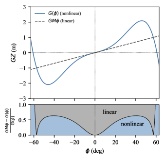
Figure 1: Nonlinear $GZ$ curve used in Duffing equation to model roll response. The lower panel shows the ratio of the nonlinear part of the curve $G(\phi)-GM\phi$ and the linear approximation $GM\phi$ to the total $GZ$.

Figure 1 shows that for roll angles larger than about 10 degrees, the nonlinear components of the restoring moment contribute greater than 25% of the total restoring moment. As a result, the true restoring moment will deviate considerably from the linear model. This is one primary reason why roll motions are strongly nonlinear at large amplitudes. In a purely linear system, the stiffening and softening of the restoring moment are not present. The linearization of the restoring moment fundamentally changes the dynamics of the model. Primarily, a nonlinear restoring moment will result in a shifting natural frequency (Wawrzyński and Krata, 2016), (Big-Alabo and Koroye, 2022), super- and sub-harmonics (Cardo et al., 1981), hysteresis (Taz Ul Mulk and Falzarano, 1994), and chaotic dynamics (Falzarano et al., 1992), (Lin and Yim, 1995), (Cotton and Spyrou, 2001).

One important consideration which is not captured by the 1-DOF Duffing equation, even with a 5th order restoring moment, is the effects of coupling with other modes of motion. Several authors have identified the importance of additional DOF for accurate roll predictions (Taz Ul Mulk and Falzarano, 1994), (Mancini et al., 2018), (Hashimoto et al., 2019). In principle, this means that the roll restoring moment cannot be modeled as a function of only roll angle, but must also include terms related to heave and pitch. The linearized coupling forces and moments are established and well-understood, but an analytical relationship of the nonlinear restoring forces and moments does not exist. Typically, the effects are considered using direct pressure integration in a high-fidelity numerical method.

2.2 Damping Moment

In a similar manner, nonlinear damping is included in Eq. (1) and parameterized by the coefficients $\alpha$, $\beta$, and $\gamma$. Cubic and quadratic damping terms are common analytical approximations of the form of the damping moment when modeling nonlinear roll responses. However, studies show that depending on the amplitude and frequency, the damping can be largely concentrated into one or all of the terms, and as with the restoring moment, the nonlinear damping terms grow much faster when roll velocity is large. Therefore, when large roll amplitudes typically coincide with large roll velocities, and nonlinear terms govern the damping moment.

If we consider Eq. (1) without the nonlinear terms, i.e. $G_{i}=0$, $i>1$ and $\beta$=$\gamma$=0, we can express the complex roll response amplitude $\bar{\phi}$ as Eq. (5), where $\bar{M}$ is the complex wave excitation amplitude which oscillates at a single angular frequency $\omega$, and $i$ is the imaginary number.

$$\bar{\phi}=\frac{\bar{M}}{-\omega^{2}+\alpha\omega i+G_{1}}$$ (5)

Now, if the excitation frequency $\omega$ is taken equivalent to the roll natural frequency $\omega_{0}=\sqrt{G_{1}}=\omega$ then Eq. (5) reduces to Eq. (6), where $|\cdot|$ indicates the amplitude of the complex argument.

$$|\bar{\phi}|=\frac{|\bar{M}|}{\alpha\omega_{0}}$$ (6)

Eq. (6) shows that the amplitude of the roll response is entirely dependent on the damping coefficient $\alpha$ when resonance occurs $\omega=\omega_{0}$. Therefore, without an accurate damping model, the obtained predictions of $|\bar{\phi}|$ will be incorrect.

Classically, roll damping is divided phenomenologically into components, such as wave radiation damping, skin friction damping, eddy damping, lift damping, and appendage damping, as introduced in the pioneering work of Ikeda et al. (1978). Potential flow methods, which assume inviscid and irrotational flow, compute only the wave radiation damping since it can be derived from the solution to the radiation problem. The radiation component is typically quite a small component of the total damping, which is why potential flow methods greatly over-predict roll responses near resonance without damping corrections. The remaining components are all due to viscous effects: skin friction is realized in the boundary layer and depends on surface roughness, eddy damping, which is often the largest damping component, is related to viscous separation around the hull as energy is lost due to the formation of vortex structures. Appendage damping is almost entirely dominated by viscous separation, as flow over bilge keels, skegs, and rudders leads to flow separation and energy dissipation.

At present, in industrial simulations, damping components are most often computed using Ikeda methods, (Ikeda et al., 1977), (Ikeda et al., 1978), (Ikeda et al., 1978), (Himeno, 1981), (Ikeda, 1983) which offer semi-empirical formulas and are relatively easy to implement alongside potential flow solvers. However, a number of researchers have identified limitations to the Ikeda methods (Haddara and Leung, 1994) and improvements are still being suggested to make the methods more applicable to a larger range of designs (Katayama and Yoshida, 2023). As a result, roll damping remains one of the greatest challenges in ship motion predictions.

2.3 Added Mass Moment of Inertia

Eq. (1) implicitly assumes linear added mass, and the equation is normalized by the total mass (including added mass), given that the coefficient of $\ddot{\phi}$ is one. However, added mass moment in roll is known to be nonlinear as well (Zhang et al., 2019), (Big-Alabo and Koroye, 2022) and can have marked impacts on the natural frequency and the effects of appendages such as bilge keels (Kianejad et al., 2019a), (Kianejad et al., 2020), (Jiang et al., 2020). While most studies linearize added mass, it is important to recognize that this may not always be an appropriate simplification.

3 Proposed Method

The proposed method is based on the neural-corrector method of Marlantes and Maki (2022), which embeds a learned data-driven force correction in a low-order equation of motion. In previous work, the method is applied to predict the heave and pitch motions of a planing boat in head seas using a synthetic data set. In the present work, the neural-corrector method is extended to model roll motions, with specific application to modeling nonlinear restoring, damping, and added mass using CFD data.

The proposed method is developed using models of ship roll at two levels of fidelity, where the superscript $(l)$ indicates low-fidelity and $(h)$ indicates high-fidelity. Under this notation, Eq. (7) is the high-fidelity model, where the solution $\phi^{(h)}$ is what we would like to obtain and is assumed to be computationally costly, i.e. derived from CFD or model testing. Eq. (8) is the low-fidelity model, where the linear added mass $A_{44}^{0}$, potential wave damping $B_{44}^{0}$, and hydrostatic restoring $C_{44}^{0}$ coefficients are computed at equilibrium. $M_{w}^{(l)}$ is the low-order wave excitation moment.

$$I_{xx}\ddot{\phi}^{(h)} =M^{(h)}$$ (7)

$$(I_{xx}+A_{44}^{0})\ddot{\phi}^{(l)}+B_{44}^{0}\dot{\phi}^{(l)}+C_{44}^{0}\phi^{(l)} =M_{w}^{(l)}$$ (8)

Eq. (9) gives the proposed hybrid equation of motion, where the superscript $*$ indicates the approximate high-fidelity state. The linearized physics are retained and a data-driven force correction, $\delta$ is included on the right-hand-side of the equation. The intent is to design $\delta$ such that the error between $\phi^{(h)}$ and $\phi^{*}$ is minimized. As shown in Marlantes and Maki (2022), $\delta$ is a complex term, including high-order contributions from the restoring, damping, and added mass moments and so it cannot be efficiently modeled using analytical techniques.

$$(I_{xx}+A_{44}^{0})\ddot{\phi}^{*}+B_{44}^{0}\dot{\phi}^{*}+C_{44}^{0}\phi^{*}=M_{w}^{(l)}+\delta(\phi^{*},\dot{\phi}^{*},\ddot{\phi}^{*})$$ (9)

In this work, the low-fidelity wave excitation $M_{w}^{(l)}$ is derived using a long-wave assumption, as given by Eq. (10). This choice is purely out of convenience, as the linear coefficients are already known. Other more accurate models can certainly be used in Eq. (9) without a loss of generality.

$$M_{w}^{(l)}=k_{w}\zeta_{w}\left((C_{44}^{0}-A_{44}^{0}\omega^{2})\cos{(\omega t)}-B_{44}^{0}\omega\sin{(\omega t)}\right)$$ (10)

The design of $\delta$ is discussed in more detail in Marlantes et al. (2023), but it is important to highlight that the term maps state variables to forces or moments, as shown in Figure 2. The term can be formulated as a function of the low-fidelity state $\phi^{(l)}$ so that a low-fidelity update is required in addition to an update to $\phi^{*}$ at each time step. However, in this work $\delta$ is designed to be a function of $\phi^{*}$ directly, making the update process fully auto-regressive. Retaining the linear force terms in the equation of motion as analytical expressions and not learning them in $\delta$ also leads to improved solution stability in the presence of errors in $\delta$, as shown in Marlantes et al. (2023).

Eq. (9) is solved numerically to obtain $\phi^{*}$, $\dot{\phi}^{*}$, $\ddot{\phi}^{*}$. To accommodate numerical integration, the machine learning model for $\delta$ follows a many-to-one paradigm, where the input features are $k$-length sequences of previous state $\phi^{*}$, $\dot{\phi}^{*}$, $\ddot{\phi}^{*}$ and the output of the model is the moment correction $\delta$ at the next time step, as shown in Figure 2. In this way, the model is trained for a particular time step size.

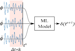
Figure 2: Design of ML model for use in neural-corrector method.

The proposed method does not require a specific ML architecture, though both Long Short-Term Memory (LSTM) and feed-forward, fully-connected neural networks have been used in prior work (Marlantes and Maki, 2022), (Marlantes et al., 2023). Because $k$ is typically less than 200 (spanning only 2 s for a timestep of 0.01 s) for typical hydrodynamic forces in marine dynamics problems, the need for memory as provided by LSTMs and Transformer networks is unnecessary and feed-forward networks with two or three layers are adequate. In this work, the ML model is a feed-forward, fully-connected neural network with 3 hidden layers, 10 nodes per layer, and ReLU activation functions.

3.1 Roll Decay Time Series as Training Data

To obtain training data for $\delta$, Eq. (9) is simply solved for $\delta$ and known high-fidelity $\phi^{(h)}$, $\dot{\phi}^{(h)}$, and $\ddot{\phi}^{(h)}$ time series are then used to compute a corresponding $\delta$ time series, as given by Eq. (11). It is therefore necessary to have an estimate of the linear coefficients for the hull under consideration, which can be obtained using a strip theory program.

$$\delta=(I_{xx}+A_{44}^{0})\ddot{\phi}^{(h)}+B_{44}^{0}\dot{\phi}^{(h)}+C_{44}^{0}\phi^{(h)}$$ (11)

Note that because the ML model is modeling forces or moments, and not the responses directly, the high-fidelity responses do not necessarily have to be the same as the expected predictions. In other words, responses computed in regular waves could be used for training data, and predictions could be made in irregular waves, for example. This is a great convenience of the proposed method. However, whatever time series are used must capture large enough amplitudes so that information about the nonlinear nature of the force or moment is embedded.

Since roll motion is the focus of the current work, it is natural to use unforced roll decay time series from a roll decay simulation or experiment as $\phi^{(h)}$ to derive $\delta$ and train the underlying ML model. Roll decay time series also intrinsically spans a range of roll amplitudes and identifies the damped natural frequency of the roll motion. Furthermore, the data are commonly available, either numerically or experimentally.

4 CFD Case of the ONR Tumblehome

To generate high-fidelity training and test data, a CFD case of a model scale (1:49) ONR Tumblehome (ONRT) hull is prepared using HELYX-OpenFOAM. The ONRT is a preliminary design of a modern surface combatant and is widely used for numerical and experimental ship hydrodynamics research. Figure 3 shows the profile view of the hull, where the sonar dome, bilgekeels, propeller shafts and struts, skeg, and rudders are visible. Table 1 gives the particulars of the ONRT model as used in this work (Bishop et al., 2005). Also given are the model scale linear added mass, potential wave damping, and hydrostatic stiffness coefficients for the equilibrium condition, which are computed using a strip theory program.

Figure 3: A profile view of the ONRT hull geometry.

Table 1: ONRT Model Particulars

Scale (-)	1:49
$L_{WL}$ (m)	3.147	Depth $D$ (m)	0.266
$B_{WL}$ (m)	0.384	Draft $T$ (m)	0.112
Mass $m$ (kg)	72.6	$A_{44}^{0}$ (kg-m2)	0.4
$I_{xx}$ (kg-m2)	1.5215	$B_{44}^{0}$ (kg-m2/s)	0.3
$V_{CG}$ (m, abl)	0.112	$C_{44}^{0}$ (kg-m2/s2)	61.5

The CFD case uses the incompressible PIMPLE algorithm to solve the Reynolds Averaged Navier-Stokes Equations (RANSE) for a multi-phase air and water domain. A Volume-of-Fluid (VOF) approach is used to capture the interface between the air and water. Variable timestepping is allowed up to a maximum Courant number of 2.0, a maximum $\alpha$-Courant number of 0.5, or a maximum timestep of 0.001 s, whichever is smaller.

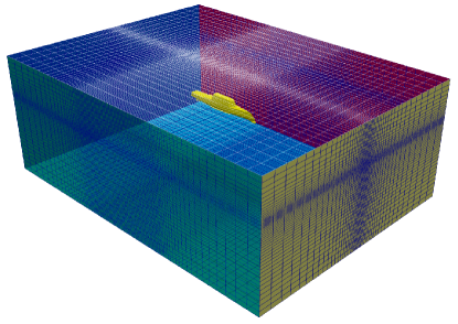
Figure 4: The computational domain used in the CFD case for the ONRT. The faces are identified by color as follows: front, back, starboard, port, top, bottom.

Figure 4 shows the computational domain, where the boundaries are colored for identification. The domain is 12.6 m long (4$L_{WL}$), 9.44 m wide (3$L_{WL}$), with water ($\alpha$=1) extending through the bottom 3.15 m ($L_{WL}$), and air ($\alpha$=0) in the top 1.51 m (0.5$L_{WL}$) following guidance in ITTC (2017). Notice the refinement in the mesh near the freesurface. Table 2 gives the boundary conditions specified on each boundary face. A $k\omega$-SST turbulence model is used, with wall functions at the hull surface.

Table 2: Boundary Conditions in ONRT CFD Case

Face	U	alpha.water	p_gh	k	omega	nut
front	symmetry	symmetry	symmetry	symmetry	symmetry	symmetry
back	symmetry	symmetry	symmetry	symmetry	symmetry	symmetry
top	press.InletOutletVelocity uniform ( 0 0 0 )	inletOutlet uniform 0	totalPressure gamma 1.4 p0 uniform 0	inletOutlet uniform 0.0002	inletOutlet uniform 0.01	calculated uniform 0.001
bottom	waveVelocity	waveAlpha	zeroGradient	fixedValue uniform 0.0002	fixedValue uniform 0.01	calculated uniform 1e-05
stbd	waveVelocity	waveAlpha	zeroGradient	turb.Int.Kin.EnergyInlet intensity 0.05 uniform 0.1	inletOutlet uniform 0.01	calculated uniform 0.001
port	waveVelocity	waveAlpha	zeroGradient	fixedValue uniform 0.0002	fixedValue uniform 0.01	calculated uniform 1e-05
hull	movingWallVelocity uniform ( 0 0 0 )	zeroGradient	fixedFluxPressure uniform 0	kqRWallFunc. uniform 1e-20	omegaWallFunc. uniform 1	nutUSpaldingWallFunc. uniform 0.001

The mesh is generated using the HelyxHexMesh utility with five extruded layers on the hull surface. The mesh is intentionally coarse, with a total of 658,473 cells. Figure 5 shows the final mesh near the hull as used in the simulations. A customized dynamic mesh method allows the input of the initial inclination of the hull for the roll decay simulation with or without forward speed. The mesh is fixed to the hull, but the entire domain is free to move with the rigid-body motion of the hull which is driven by the fluid forces acting on the hull patches. To initialize the roll decay simulations, the dynamic mesh is ramped up to the desired inclination over a 1 s interval before the mesh is released.

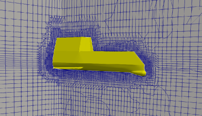
Figure 5: A view of the unstructured hexahedral mesh used to simulate the roll response of the ONRT. The mesh is intentionally coarse, with a total count of 658,473 cells.

Figure 6 shows roll decay time series obtained from the CFD case for three different initial conditions: inclinations of 5 degrees, 10 degrees, and 20 degrees. The total time series length for a single simulation is 20 seconds. Also shown in the figure are the resulting force correction time series, computed using Eq. (11) and the linear coefficients given in Table 1. The responses $\phi^{(h)}$, $\dot{\phi}^{(h)}$, $\ddot{\phi}^{(h)}$ and corresponding $\delta$ in Figure 6 comprise the entire training data set available to train the ML model. However, training on all three time series proves to be less effective than training on only the $\phi_{0}$=20 deg case, likely due to the lack of nonlinear variation in the small amplitude cases. Therefore, the final training data set consists of only the $\phi_{0}$=20 deg decay simulation: a total of 20 seconds of time series with a downsampled time step of 0.001 seconds.

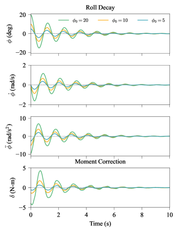
Figure 6: Roll decay time series $\phi^{(h)}$, $\dot{\phi}^{(h)}$, $\ddot{\phi}^{(h)}$ of the ONRT at zero forward speed computed using the CFD case for use as training data in Eq. (11). Three different initial conditions are shown: $\phi_{0}$=5 deg, 10 deg, and 20 deg, however, only the $\phi_{0}$=20 deg case is used for training data.

In addition to the roll decay simulations, roll responses in five different wave periods, 1.00 s, 1.14 s, 1.25 s, 1.39 s, and 2.00 s, all using a wave amplitude of 0.05 m are simulated using the same domain and model set up as the roll decay simulations. The responses are generated not as training data, but as validation data to test the accuracy of the proposed method. Regular waves are generated using the waves2Foam toolbox, which utilizes a relaxation zone technique to enforce the wave velocity and $\alpha$-field in the inlet and outlet regions (Jacobsen et al., 2012). Two rectangular relaxation zones, one on the starboard side inlet, and one on the port side outlet, are specified, with the inboard edge of the relaxation zones extending to 1.0 m off the centerline of the domain, or about 2.25$B_{WL}$ from the side of the hull. A spatial-implicit relaxation scheme is used and the relaxation weights are specified using a third-order polynomial.

5 Results

The roll decay data for $\phi_{0}$=20 deg from Figure 6 are used to train a feed-forward, fully connected neural network model as described in Section 3. A stencil-length of $k$=5 is selected for the configuration, which corresponds to 0.005 seconds with a 0.001 s timestep. The model is trained using the Adam optimizer (Kingma and Ba, 2014) and a Mean-Squared-Error (MSE) loss function for up to 1000 epochs, stopping early when the loss does not improve greater than 1e-04 after ten consecutive iterations. Figure 7 shows the training loss for the model.

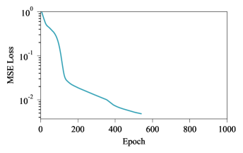
Figure 7: Training loss for a feed-forward, fully-connected neural network with 3 hidden layers, 10 nodes per layer, reLU activation functions. The model learns the many-to-one relationship between $k$-length sequences of the state variables $\phi$, $\dot{\phi}$, $\ddot{\phi}$ at $t=n-k..n$ and the force correction $\delta$ at $t=n+1$ for $k=5$.

Using the trained model, Eq. (9) is solved numerically using a first-order forward Euler scheme. To check that the learned force correction is indeed performing as expected within the integration scheme, Eq. (9) is first solved without external forcing (i.e. $M_{w}^{(l)}=0$) using the same initial conditions that are used in the CFD simulations in Section 4. Figure 8 shows the solution for the initial condition $\phi_{0}$=20 deg. As expected, the proposed method closely follows the high-fidelity CFD decay time series.

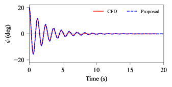
Figure 8: Roll decay time series comparison between the CFD results $\phi^{(h)}$ and the proposed model $\phi^{*}$ of the ONRT at zero forward speed for initial condition $\phi_{0}$=20 deg.

Reproducing the training data time series is encouraging, however, the proposed method is not useful if it cannot be used in conditions that differ from the training data set. Furthermore, the method must perform well in the presence of wave excitation moments, since the primary objective of this work is to develop a model which can be used to efficiently assess the roll motion of a ship in waves. To test this, the wave excitation moment $M_{w}^{(l)}$ is modeled using Eq. (10) using the linear coefficients from Table 1. Eq. (9) is solved for wave frequencies ranging from 2.0 to 12.0 rad$\cdot$s^-1 with a constant wave amplitude of 0.05 m and at-rest initial conditions of $\phi_{0}$=$\dot{\phi}_{0}$=$\ddot{\phi}_{0}$=0. The steady-state peak responses from each time domain solution are used to compute the RAO of the response, normalized by the wave slope $k_{w}\zeta_{w}$. The resulting RAO is shown in Figure 9 alongside the regular wave results that are computed using the CFD case. Also shown is the linear RAO, computed using strip theory, for the same loading condition.

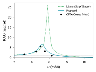
Figure 9: Predicted forced roll response RAO for the ONRT at zero forward speed in regular waves over a range of wave excitation frequencies.

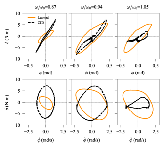
Figure 10: Lissajous curves for the learned and CFD-derived $\delta$ vs $\phi$, $\dot{\phi}$, and $\ddot{\phi}$ through one period for the ONRT at zero forward speed in regular waves. Results are given for $\omega/\omega_{0}$=0.87, 0.94, and 1.05 to show the behavior around the natural frequency and to correspond with the CFD regular wave cases.

Figure 9 shows that the proposed method greatly improves the predicted amplitudes of forced responses when compared to the linear benchmark, especially in regions near the natural frequency $\omega_{0}$. In general, the results are in fair agreement with the CFD cases. The captured shift in the natural frequency suggests the ML model imparts corrections to both the roll restoring and added mass moments, and the reduced amplitude near the natural frequency is indicative of corrections to the damping moment. The large shift may also be attributed to the effects of the appendages, which are present in the proposed model. The model still reproduces the long- and short-wave limits of the linear model, which indicates that the learned moments vanish in wave conditions which are dominantly linear.

However, the learned model over-predicts the amplitude of the response at wave excitation frequencies that are above the natural frequency, in a region where the mass terms of Eq. (9) dominate. It is important to note that the wave excitation model given by Eq. (10) makes a long-wave assumption, which could be partly responsible for the deviation, but the extent of this assumption is not known. To investigate this behavior further, Figure 10 shows the Lissajous curves for the predicted and CFD-derived roll moment correction $\delta$ against the predicted state $\phi$, $\dot{\phi}$, and $\ddot{\phi}$ for three cases around the natural frequency: $\omega/\omega_{0}$=0.87, 0.94, and 1.05. The progression of each curve is in the counter-clockwise direction. The curves are useful because they magnify any differences in phase and magnitude to make the underlying dynamics more apparent. One should keep in mind, however, that the CFD-derived moment also includes nonlinearity imparted by the incident waves and interacting radiated waves–a potentially major contribution which is not present in the learned model due to the unforced training data set.

In the $\omega/\omega_{0}$=0.94 wave case, which is the closest to the natural frequency of the three cases, both the magnitude and phase of the predicted moment correction are closest to the CFD-derived counterparts. It is also shown that the CFD-derived moments are primarily in phase with the position, and about 90^∘ out of phase with the velocity. The spread of the predicted moments along the vertical axis indicates a negative (lagging) phase shift with respect to position. In the higher-frequency $\omega/\omega_{0}$=1.05 case, the ML model is considerably over-predicting the amplitude of the moment correction and a phase error is also present. This is likely the reason for the over-prediction in the response amplitude shown in Figure 9, as the phase angle may lead to an amplification of the response, instead of an attenuation. In the lower-frequency $\omega/\omega_{0}$=0.87 case, the amplitude of the predicted $\delta$ decreases significantly yet the phase agreement remains fair. Despite this, the small amplitude does not significantly affect the predictions as this region of the response is dominated by restoring forces, and the CFD-derived corrections show an almost purely linear form in phase with position.

Of interest in Figure 10 is the asymmetry in almost all of the curves, which differs strongly from classical linear-quadratic or linear-cubic models, especially in the higher-frequency case. The asymmetry may be partly attributed to nonlinear variation in the added mass, which is known to be asymmetric (Big-Alabo and Koroye, 2022). The non-zero correction for the CFD-derived values at $\phi$=$\dot{\phi}$=$\ddot{\phi}$=0, especially in the higher-frequency case, is also attributable to a known mean-shift in the nonlinear responses in waves (Big-Alabo and Koroye, 2022).

The comparison in Figure 10 exposes some weaknesses when training on only unforced responses such as roll decay time series, which is noted by other studies (Somayajula and Falzarano, 2017), (Rodríguez et al., 2020). Foremost is the trained models reduced ability to learn phase, as evidenced by the weak phase shift across the three frequencies. In addition, the over-prediction of the moment correction in the higher-frequencies suggests that while training at $\omega_{0}$ captures the damping moments at the most critical frequencies, the predictions could be improved by training in forced responses at two or more frequencies. However, this should not diminish the practicality of unforced roll decay time series as a training data set, especially when derived from experiments, given the considerable improvement of the RAO in Figure 9.

6 Conclusions

In this work, the neural-corrector method of Marlantes and Maki (2022) is extended to model roll motions of an ONRT hull at model scale in regular waves. The hybrid data-driven method is trained using unforced roll decay time series data generated using CFD. Several conclusions can be drawn from the work:

• When trained on roll decay data, the proposed method learns a significant component of the nonlinear added mass, restoring, and damping moments. The effects of appendages, such as bilge keels, are also included.

• Though the training data set is only unforced roll decay time series, the proposed method greatly improves predictions of forced responses in waves, with fair agreement compared to CFD validation data.

• The proposed model reproduces the long- and short-wave limits of the linear model, indicating that the learned moments vanish in wave conditions which are dominantly linear.

• The model is inexpensive to evaluate with a computational cost of approximately 5% real-time.

• The model is practical. The training data set consists of only a single, 20-second CFD roll decay simulation and linear coefficients computed using frequency-domain strip theory.

However, there are a couple limitations which should be mentioned. First, the model, as proposed, is sensitive to the accuracy of the low-fidelity wave excitation model in Eq. (9). To overcome this limitation, the force correction in Marlantes and Maki (2022) captures components of the nonlinear wave excitation force and the wave elevation is included as an additional input feature in the ML model. However, this also requires training data from roll responses in the presence of waves, which differs from the unforced roll decay data used in the present work. If forced responses were used for training data, time series from responses in two or more regular wave frequencies–or perhaps irregular waves, which encompass many frequencies–may also improve the predicted moments in Fig. 10. Second, this study considered only 1-DOF roll motion, specifically due to its similarity to classical parameter identification methods, but should be extended to at least 3-DOF (heave, sway, roll) to capture the influence of coupling with other modes. However, free decay data is only available for modes of motion which have a restoring force. For modes such as sway, a forced approach would be required to generate the training data.

References

- Aloisio and Felice (2006) Aloisio, G., Felice, F., 2006. Piv analysis around the bilge keel of a ship model in free roll decay. Roma, Italia, XIV Convegno Nazionale AI VE. LA 1.
- Avalos et al. (2014) Avalos, G.O., Wanderley, J.B., Fernandes, A.C., Oliveira, A.C., 2014. Roll damping decay of a fpso with bilge keel. Ocean Engineering 87, 111–120. URL: https://www.sciencedirect.com/science/article/pii/S0029801814001863, doi:https://doi.org/10.1016/j.oceaneng.2014.05.008.
- Bagazinski and Ahmed (2023) Bagazinski, N.J., Ahmed, F., 2023. Ship-d: Ship hull dataset for design optimization using machine learning. URL: https://browse.arxiv.org/pdf/2305.08279.pdf.
- Bassler et al. (2010) Bassler, C., Reed, A., Brown, A.J., 2010. A method to model large amplitude ship roll damping, in: Proceedings of the 11th International Ship Stability Workshop, pp. 217–224.
- Begovic et al. (2015) Begovic, E., Day, A.H., Incecik, A., Mancini, S., Pizzirusso, D., et al., 2015. Roll damping assessment of intact and damaged ship by cfd and efd methods, in: Proceedings of the 12th international conference on the stability of ships and ocean vehicles, Glasgow, UK, pp. 14–19.
- Big-Alabo and Koroye (2022) Big-Alabo, A., Koroye, D., 2022. Nonlinear vibration analysis of the large-amplitude asymmetric response of ship roll motion. Ocean Engineering 243, 110088. URL: https://www.sciencedirect.com/science/article/pii/S0029801821014153, doi:https://doi.org/10.1016/j.oceaneng.2021.110088.
- Bishop et al. (2005) Bishop, R.C., Belknap, W., Turner, C., Simon, B., Kim, J.H., 2005. Parametric investigation on the influence of gm, roll damping, and above-water form on the roll response of model 5613. Hydromechanics Department, Naval Surface Warfare Center Carderock Division, West Bethesda, Maryland, USA, Report NSWCCD-50-TR-2005/027 .
- Cardo et al. (1981) Cardo, A., Francescutto, A., Nabergoj, R., 1981. Ultraharmonics and subharmonics in the rolling motion of a ship: Steady-state solution , 234–251.
- Chan et al. (1995) Chan, H., Xu, Z., Huang, W., 1995. Estimation of nonlinear damping coefficients from large-amplitude ship rolling motions. Applied Ocean Research 17, 217–224. URL: https://www.sciencedirect.com/science/article/pii/0141118795000240, doi:https://doi.org/10.1016/0141-1187(95)00024-0.
- Chen et al. (2019) Chen, C., Tello Ruiz, M., Delefortrie, G., Mei, T., Vantorre, M., Lataire, E., 2019. Parameter estimation for a ship’s roll response model in shallow water using an intelligent machine learning method. Ocean Engineering 191, 106479. URL: https://www.sciencedirect.com/science/article/pii/S0029801819306225, doi:https://doi.org/10.1016/j.oceaneng.2019.106479.
- Copuroglu et al. (2023) Copuroglu, H.I., Pesman, E., Morata, H., Yoshida, N., Yamamoto, Y., Katayama, T., 2023. Experimental and numerical investigation of viscous effects on parametric roll motion, in: Proceedings of the 19th International Ship Stability Workshop, Istanbul, Turkey.
- Cotton and Spyrou (2001) Cotton, B., Spyrou, K., 2001. An experimental study of nonlinear behaviour in roll and capsize. International shipbuilding progress 48, 5–18.
- Dalzell (1978) Dalzell, J., 1978. A note on the form of ship roll damping. Journal of Ship Research 22, 178–185.
- Eissa and El-Bassiouny (2003) Eissa, M., El-Bassiouny, A., 2003. Analytical and numerical solutions of a non-linear ship rolling motion. Applied Mathematics and Computation 134, 243–270. URL: https://www.sciencedirect.com/science/article/pii/S009630030100279X, doi:https://doi.org/10.1016/S0096-3003(01)00279-X.
- Falzarano et al. (2015) Falzarano, J., Somayajula, A., Seah, R., 2015. An overview of the prediction methods for roll damping of ships. Ocean Systems Engineering 5, 55–76.
- Falzarano et al. (1992) Falzarano, J.M., Shaw, S.W., Troesch, A.W., 1992. Application of global methods for analyzing dynamical systems to ship rolling motion and capsizing. International Journal of Bifurcation and Chaos 02, 101–115. doi:10.1142/S0218127492000100.
- Froude (1861) Froude, W., 1861. On the rolling of ships. 2nd Session of the Institution of Naval Architects, March 1861 .
- Gokce and Kinaci (2018) Gokce, M.K., Kinaci, O.K., 2018. Numerical simulations of free roll decay of dtmb 5415. Ocean Engineering 159, 539–551. URL: https://www.sciencedirect.com/science/article/pii/S0029801817308053, doi:https://doi.org/10.1016/j.oceaneng.2017.12.067.
- Haddara and Leung (1994) Haddara, M., Leung, S., 1994. Experimental investigation of the lift component of roll damping. Ocean Engineering 21, 115–127. URL: https://www.sciencedirect.com/science/article/pii/0029801894900345, doi:https://doi.org/10.1016/0029-8018(94)90034-5.
- Handschel and Abdel-Maksoud (2014) Handschel, S., Abdel-Maksoud, M., 2014. Improvement of the harmonic excited roll motion technique for estimating roll damping. Ship Technology Research 61, 116–130.
- Hashimoto et al. (2019) Hashimoto, H., Omura, T., Matsuda, A., Yoneda, S., Stern, F., Tahara, Y., 2019. Several remarks on efd and cfd for ship roll decay. Ocean Engineering 186, 106082. URL: https://www.sciencedirect.com/science/article/pii/S0029801819302847, doi:https://doi.org/10.1016/j.oceaneng.2019.05.064.
- Himeno (1981) Himeno, Y., 1981. Prediction of ship roll damping-a state of the art .
- Ikeda (1983) Ikeda, Y., 1983. On the form of non-linear roll damping of ships. University of Osaka Prefacture, Department of Naval Architecture, Japan, Report No. 00406, Published by: Technische Universität Berlin, Germany, Institut für Schiffs-und Meerestechnik, ISM Bericht 83/15 .
- Ikeda et al. (1977) Ikeda, Y., Himeno, Y., Tanaka, N., 1977. On eddy making component of roll damping force on naked hull. Journal of the society of Naval Architects of Japan 1977, 54–64.
- Ikeda et al. (1978) Ikeda, Y., Himeno, Y., Tanaka, N., 1978. Components of roll damping of ship at forward speed. Journal of the society of Naval Architects of Japan 1978, 113–125.
- Irkal et al. (2016) Irkal, M.A., Nallayarasu, S., Bhattacharyya, S., 2016. Cfd approach to roll damping of ship with bilge keel with experimental validation. Applied Ocean Research 55, 1–17. URL: https://www.sciencedirect.com/science/article/pii/S0141118715001509, doi:https://doi.org/10.1016/j.apor.2015.11.008.
- Irkal et al. (2019) Irkal, M.A., Nallayarasu, S., Bhattacharyya, S., 2019. Numerical prediction of roll damping of ships with and without bilge keel. Ocean Engineering 179, 226–245. URL: https://www.sciencedirect.com/science/article/pii/S0029801818315658, doi:https://doi.org/10.1016/j.oceaneng.2019.03.027.
- ITTC (2017) ITTC, 2017. Recommended procedures and guidelines - practical guidelines for ship cfd applications.
- Jacobsen et al. (2012) Jacobsen, N.G., Fuhrman, D.R., Fredsøe, J., 2012. A wave generation toolbox for the open-source cfd library: Openfoam®. International Journal for numerical methods in fluids 70, 1073–1088.
- Jang et al. (2010) Jang, T., Kwon, S., Lee, J., 2010. Recovering the functional form of the nonlinear roll damping of ships from a free-roll decay experiment: An inverse formulism. Ocean Engineering 37, 1337–1344. URL: https://www.sciencedirect.com/science/article/pii/S0029801810001460, doi:https://doi.org/10.1016/j.oceaneng.2010.06.012.
- Jiang et al. (2020) Jiang, Y., Ding, Y., Sun, Y., Shao, Y., Sun, L., 2020. Influence of bilge-keel configuration on ship roll damping and roll response in waves. Ocean Engineering 216, 107539. URL: https://www.sciencedirect.com/science/article/pii/S0029801820305503, doi:https://doi.org/10.1016/j.oceaneng.2020.107539.
- Katayama and Yoshida (2023) Katayama, T., Yoshida, N., 2023. Effects of height of roll axis on pressure distribution on hull caused by bilge-keels, in: Proceedings of the 19th International Ship Stability Workshop, Istanbul, Turkey.
- Kianejad et al. (2019a) Kianejad, S., Enshaei, H., Duffy, J., Ansarifard, N., 2019a. Prediction of a ship roll added mass moment of inertia using numerical simulation. Ocean Engineering 173, 77–89. URL: https://www.sciencedirect.com/science/article/pii/S002980181831429X, doi:https://doi.org/10.1016/j.oceaneng.2018.12.049.
- Kianejad et al. (2020) Kianejad, S., Enshaei, H., Duffy, J., Ansarifard, N., 2020. Calculation of ship roll hydrodynamic coefficients in regular beam waves. Ocean Engineering 203, 107225. URL: https://www.sciencedirect.com/science/article/pii/S0029801820302808, doi:https://doi.org/10.1016/j.oceaneng.2020.107225.
- Kianejad et al. (2018) Kianejad, S., Enshaei, H., Duffy, J., Ansarifard, N., Ranmuthugala, D., 2018. Investigation of scale effects on roll damping through numerical simulations, in: 32nd Symposium on Naval Hydrodynamics, pp. 5–10.
- Kianejad et al. (2019b) Kianejad, S.S., Enshaei, H., Duffy, J., Ansarifard, N., Ranmuthugala, D., 2019b. Ship roll damping coefficient prediction using cfd. Journal of Ship Research 63, 108–122.
- Kim and Park (2015) Kim, Y., Park, M.J., 2015. Identification of the nonlinear roll damping and restoring moment of a fpso using hilbert transform. Ocean Engineering 109, 381–388. URL: https://www.sciencedirect.com/science/article/pii/S0029801815004916, doi:https://doi.org/10.1016/j.oceaneng.2015.09.019.
- Kingma and Ba (2014) Kingma, D.P., Ba, J., 2014. Adam: A method for stochastic optimization. URL: https://arxiv.org/abs/1412.6980, doi:10.48550/ARXIV.1412.6980.
- Korpus and Falzarano (1997) Korpus, R.A., Falzarano, J.M., 1997. Prediction of viscous ship roll damping by unsteady navier-stokes techniques .
- Lin and Yim (1995) Lin, H., Yim, S.C., 1995. Chaotic roll motion and capsize of ships under periodic excitation with random noise. Applied Ocean Research 17, 185–204. URL: https://www.sciencedirect.com/science/article/pii/0141118795000143, doi:https://doi.org/10.1016/0141-1187(95)00014-3.
- Maki et al. (2022) Maki, A., Dostal, L., Maruyama, Y., Sasa, K., Sakai, M., Umeda, N., 2022. Enhanced estimation method and approximation method of the pdf of roll angular acceleration and jerk in beam seas. Ocean Engineering 264, 112159. URL: https://www.sciencedirect.com/science/article/pii/S0029801822014755, doi:https://doi.org/10.1016/j.oceaneng.2022.112159.
- Mancini et al. (2018) Mancini, S., Begovic, E., Day, A.H., Incecik, A., 2018. Verification and validation of numerical modelling of dtmb 5415 roll decay. Ocean Engineering 162, 209–223. URL: https://www.sciencedirect.com/science/article/pii/S0029801818308205, doi:https://doi.org/10.1016/j.oceaneng.2018.05.031.
- Marlantes et al. (2023) Marlantes, K.E., Bandyk, P.J., Maki, K.J., 2023. Investigating nonlinear forces in ship dynamics using machine learning, in: Proceedings of the 10th International Conference on Computational Methods in Marine Engineering (MARINE), Madrid, Spain.
- Marlantes et al. (2022) Marlantes, K.E., Kim, S.P., Hurt, L.A., 2022. Implementation of the imo second generation intact stability guidelines. Journal of Marine Science and Engineering 10. URL: https://www.mdpi.com/2077-1312/10/1/41, doi:10.3390/jmse10010041.
- Marlantes and Maki (2021) Marlantes, K.E., Maki, K.J., 2021. Modeling vertical planing boat motions using a neural-corrector method, in: SNAME International Conference on Fast Sea Transportation, SNAME. p. D011S002R005.
- Marlantes and Maki (2022) Marlantes, K.E., Maki, K.J., 2022. A neural-corrector method for prediction of the vertical motions of a high-speed craft. Ocean Engineering 262, 112300. URL: https://www.sciencedirect.com/science/article/pii/S0029801822015967, doi:https://doi.org/10.1016/j.oceaneng.2022.112300.
- Matsui et al. (2023) Matsui, S., Sugimoto, K., Shinomoto, K., 2023. Simplified estimation formula for frequency response function of roll motion of ship in waves. Ocean Engineering 276, 114187. URL: https://www.sciencedirect.com/science/article/pii/S0029801823005711, doi:https://doi.org/10.1016/j.oceaneng.2023.114187.
- Nayfeh and Sanchez (1989) Nayfeh, A.H., Sanchez, N.E., 1989. Bifurcations in a forced softening duffing oscillator. International Journal of Non-Linear Mechanics 24, 483–497. URL: https://www.sciencedirect.com/science/article/pii/0020746289900140, doi:https://doi.org/10.1016/0020-7462(89)90014-0.
- Oliva-Remola et al. (2018) Oliva-Remola, A., Bulian, G., Pérez-Rojas, L., 2018. Estimation of damping through internally excited roll tests. Ocean Engineering 160, 490–506. URL: https://www.sciencedirect.com/science/article/pii/S0029801818305419, doi:https://doi.org/10.1016/j.oceaneng.2018.04.052.
- Rajaraman and Hariharan (2023) Rajaraman, R., Hariharan, G., 2023. Estimation of roll damping parameters using hermite wavelets: An operational matrix of derivative approach. Ocean Engineering 283, 115031. URL: https://www.sciencedirect.com/science/article/pii/S0029801823014154, doi:https://doi.org/10.1016/j.oceaneng.2023.115031.
- Roberts et al. (1994) Roberts, J., Dunne, J., Debonos, A., 1994. Stochastic estimation methods for non-linear ship roll motion. Probabilistic Engineering Mechanics 9, 83–93. URL: https://www.sciencedirect.com/science/article/pii/0266892094900329, doi:https://doi.org/10.1016/0266-8920(94)90032-9.
- Roberts (1985) Roberts, J.B., 1985. Estimation of nonlinear ship roll damping from free-decay data. Journal of Ship Research 29, 127–138.
- Rodríguez et al. (2020) Rodríguez, C.A., Ramos, I.S., Esperança, P.T., Oliveira, M.C., 2020. Realistic estimation of roll damping coefficients in waves based on model tests and numerical simulations. Ocean Engineering 213, 107664. URL: https://www.sciencedirect.com/science/article/pii/S0029801820306612, doi:https://doi.org/10.1016/j.oceaneng.2020.107664.
- Schirmann et al. (2022) Schirmann, M.L., Collette, M.D., Gose, J.W., 2022. Data-driven models for vessel motion prediction and the benefits of physics-based information. Applied Ocean Research 120, 102916. URL: https://www.sciencedirect.com/science/article/pii/S0141118721003850, doi:https://doi.org/10.1016/j.apor.2021.102916.
- Schirmann et al. (2023) Schirmann, M.L., Gose, J.W., Collette, M.D., 2023. A comparison of physics-informed data-driven modeling architectures for ship motion predictions. Ocean Engineering 286, 115608. URL: https://www.sciencedirect.com/science/article/pii/S0029801823019923, doi:https://doi.org/10.1016/j.oceaneng.2023.115608.
- Skulstad et al. (2021) Skulstad, R., Li, G., Fossen, T.I., Vik, B., Zhang, H., 2021. A hybrid approach to motion prediction for ship docking—integration of a neural network model into the ship dynamic model. IEEE Transactions on Instrumentation and Measurement 70, 1–11. doi:10.1109/TIM.2020.3018568.
- Somayajula and Falzarano (2017) Somayajula, A., Falzarano, J., 2017. Application of advanced system identification technique to extract roll damping from model tests in order to accurately predict roll motions. Applied Ocean Research 67, 125–135. URL: https://www.sciencedirect.com/science/article/pii/S0141118717302316, doi:https://doi.org/10.1016/j.apor.2017.07.007.
- Spyrou et al. (2008) Spyrou, K.J., Niotis, S., Panagopoulou, C., 2008. ‘novel modeling of ship rolling based on fractional calculus, in: The 6th OSAKA Colloquium on Seakeeping and Stability of Ships (5), pp. 1–8.
- Spyrou and Thompson (2000) Spyrou, K.J., Thompson, J.M.T., 2000. The nonlinear dynamics of ship motions: a field overview and some recent developments. Phil. Trans. R. Soc. A. 358, 1735–1760.
- Suliman and Thompson (1991) Suliman, M., Thompson, J., 1991. Transient and steady state analysis of capsize phenomena. Applied Ocean Research 13, 82–92.
- Sun et al. (2021) Sun, J., James Hu, S.L., Li, H., 2021. Nonlinear roll damping parameter identification using free-decay data. Ocean Engineering 219, 108425. URL: https://www.sciencedirect.com/science/article/pii/S0029801820313329, doi:https://doi.org/10.1016/j.oceaneng.2020.108425.
- Taylan (2000) Taylan, M., 2000. The effect of nonlinear damping and restoring in ship rolling. Ocean Engineering 27, 921–932. URL: https://www.sciencedirect.com/science/article/pii/S0029801899000268, doi:https://doi.org/10.1016/S0029-8018(99)00026-8.
- Taz Ul Mulk and Falzarano (1994) Taz Ul Mulk, M., Falzarano, J., 1994. Complete Six-Degrees-of-Freedom Nonlinear Ship Rolling Motion. Journal of Offshore Mechanics and Arctic Engineering 116, 191–201. URL: https://doi.org/10.1115/1.2920150, doi:10.1115/1.2920150.
- Wan et al. (2018) Wan, Z.Y., Vlachas, P., Koumoutsakos, P., Sapsis, T., 2018. Data-assisted reduced-order modeling of extreme events in complex dynamical systems. PLOS ONE 13, 1–22.
- Wassermann et al. (2016) Wassermann, S., Feder, D.F., Abdel-Maksoud, M., 2016. Estimation of ship roll damping—a comparison of the decay and the harmonic excited roll motion technique for a post panamax container ship. Ocean Engineering 120, 371–382. URL: https://www.sciencedirect.com/science/article/pii/S0029801816000640, doi:https://doi.org/10.1016/j.oceaneng.2016.02.009.
- Wawrzynski (2023) Wawrzynski, W., 2023. Ship rolling equation: Comparison of the different damping models. Ocean Engineering 280, 114760. URL: https://www.sciencedirect.com/science/article/pii/S0029801823011447, doi:https://doi.org/10.1016/j.oceaneng.2023.114760.
- Wawrzyński and Krata (2016) Wawrzyński, W., Krata, P., 2016. On ship roll resonance frequency. Ocean Engineering 126, 92–114. URL: https://www.sciencedirect.com/science/article/pii/S0029801816303602, doi:https://doi.org/10.1016/j.oceaneng.2016.08.026.
- Weymouth and Yue (2014) Weymouth, G., Yue, D.K.P., 2014. Physics-based learning models for ship hydrodynamics. Journal of Ship Research 57.
- Willard et al. (2020) Willard, J., Jia, X., Xu, S., Steinbach, M., Kumar, V., 2020. Integrating physics-based modeling with machine learning: A survey. arXiv:2003.04919.
- Wilson et al. (2006) Wilson, R.V., Carrica, P.M., Stern, F., 2006. Unsteady rans method for ship motions with application to roll for a surface combatant. Computers and Fluids 35, 501--524. URL: https://www.sciencedirect.com/science/article/pii/S0045793005000526, doi:https://doi.org/10.1016/j.compfluid.2004.12.005.
- Yang et al. (2022) Yang, K., Duan, W., Huang, L., Zhang, P., Ma, S., 2022. A prediction method for ship added resistance based on symbiosis of data-driven and physics-based models. Ocean Engineering 260, 112012. URL: https://www.sciencedirect.com/science/article/pii/S0029801822013439, doi:https://doi.org/10.1016/j.oceaneng.2022.112012.
- Yu et al. (2022) Yu, Y., Song, W., Zhao, P., Li, Z., 2022. Approximate analytical investigation of large-amplitude rolling motion of ships with the improved galerkin method. Ocean Engineering 266, 112855. URL: https://www.sciencedirect.com/science/article/pii/S0029801822021382, doi:https://doi.org/10.1016/j.oceaneng.2022.112855.
- Zhang et al. (2023) Zhang, D., Wang, W., Bu, S., Liu, W., 2023. Formulation of ship roll damping models from free-decay data. Ocean Engineering 280, 114658. URL: https://www.sciencedirect.com/science/article/pii/S0029801823010429, doi:https://doi.org/10.1016/j.oceaneng.2023.114658.
- Zhang et al. (2019) Zhang, X., Gu, X., Ma, N., 2019. Prediction of roll hydrodynamic characteristics for a ship hull section with a high-order finite volume solver. Ocean Engineering 180, 119--129. URL: https://www.sciencedirect.com/science/article/pii/S0029801818320171, doi:https://doi.org/10.1016/j.oceaneng.2019.04.012.