Probe particles in odd active viscoelastic fluids: how activity and dissipation determine linear stability

Abstract

Odd viscoelastic materials are constrained by fewer symmetries than their even counterparts. The breaking of these symmetries allow these materials to exhibit different features, which have attracted considerable attention in recent years. Immersing a bead in such complex fluids allows for probing their physical properties, highlighting signatures of their oddity and exploring consequences of these broken symmetries. We present the conditions under which the activity of an odd viscoelastic fluid can give rise to linear instabilities in the motion of the probe particle and unveil how the features of the probe particle dynamics depend on the oddity and activity of the viscoelastic medium in which it is immersed.

Introduction

Chiral two-dimensional materials break parity symmetry and display transport phenomena characterized by tensors that are odd under index exchange. Such odd systems attract considerable interests from a broad range of communities. These include soft active matter, statistical physics and biological physics Epstein and Mandadapu (2020); Hargus et al. (2020); Lier et al. (2022); Han et al. (2021); Hargus et al. (2021); Soni et al. (2019); Reichhardt and Reichhardt (2019); Markovich and Lubensky (2021); Reichhardt and Reichhardt (2022); Fürthauer et al. (2012); Tan et al. (2022); Banerjee et al. (2021); Surówka et al. (2022); Kalz et al. (2023, 2022), fluid dynamics Banerjee et al. (2017); Abanov et al. (2018); Ganeshan and Abanov (2017); Khain et al. (2022); Hosaka et al. (2023a, 2021a, b), complex materials Scheibner et al. (2020); Braverman et al. (2021); Floyd et al. (2022); Fruchart et al. (2022); Liao et al. (2020), electron fluids Pellegrino et al. (2017); Narozhny and Schütt (2019); Berdyugin et al. (2019), and topological waves Fossati et al. (2022); Green et al. (2020); Souslov et al. (2019); Tauber et al. (2019). Recent experiments have begun measuring odd systems  Berdyugin et al. (2019); Soni et al. (2019); Tan et al. (2022); Bililign et al. (2022). One of these odd phenomena is odd elasticity Scheibner et al. (2020); Tan et al. (2022). Odd elastic solids can perform net work under quasi-static cycles, implying that they are active materials, as such phenomena can only occur in the presence of a constant energy injection at the microscopic level. Such energy injection, if not properly dissipated, can give rise to linear instabilities Floyd et al. (2022); Scheibner et al. (2020). Complex materials that exhibit elastic properties at short times and fluid-like ones at long times are called viscoelastic. Odd viscoelastic systems were first discussed in Banerjee et al. (2021) in the context of active matter and recently shown to exist also in a passive context, provided that certain thermodynamic constraints are obeyed Lier et al. (2022).

A powerful method of probing the physical properties of a fluid is to observe the motion of a probe particle immersed in it Mason and Weitz (1995); MacKintosh and Schmidt (1999); Squires and Mason (2010). This is even more important for active odd viscoelastic materials. First, because the response contains signatures of the odd nature of the material, such as odd lift forces Lier et al. (2023); Hosaka et al. (2021b). Second, because the viscoelastic nature of the system makes the response in time to instantaneous external perturbations non-trivial Gardel et al. (2005). Third, because activity can give rise to sustained motion of the probe particle and, potentially, instability in the response to perturbations (see, e.g., Ref. Di Leonardo et al. (2010)).

Figure 1: Schematic picture of a probe particle moving with velocity $U$ in an odd viscoelastic fluid, experiencing a drag force $F_{\parallel}$ and a lift force $F_{\perp}$.

In this work, we shed light on these three points by looking at the motion of a passive probe particle in an active odd viscoelastic fluid (see Fig. 1). First, we derive the material properties of such a fluid from Onsager’s theory, and show that activity introduces interesting physics by breaking the Onsager-symmetry and thermodynamic inequalities that otherwise constrain the stress-strain relations. We then unveil the conditions that grant the stability of the motion of the probe particle when it is embedded in an active fluid. After confirming that a probe in a passive system has a stable trajectory, i.e. its velocity decays at long times, we show that, within our linear approach, there exists an intermediate regime where the probe motion through an active systems is still stable. For larger activities, a probe that is subjected to an external force at an initial time becomes linearly unstable. We also focus on the signatures of oddity, which can be seen in the dynamics of the probe. We observe that odd viscoelastic terms promote long-lasting oscillations during the relaxation process after an instantaneous perturbation. These findings provide tools to assess the degree of oddity of a material by studying the motion of a probe inserted in it.

I probe particle in an active odd viscoelastic fluid

I.1 Constitutive equations for the fluid

In this Section, we discuss the material properties of the two-dimensional odd viscoelastic fluid in which the probe particle moves. For this purpose, we start with the total stress tensor $\underline{\underline{\sigma}}^{\rm tot}$, which enters the momentum balance equation as

$$\partial_{t}\mathbf{g}-\nabla\cdot\underline{\underline{\sigma}}^{\rm tot}=\mathbf{f}^{\rm{ext}}\,.$$ (1)

We have introduced the momentum $\mathbf{g}=\rho\mathbf{v}$ with $\rho$ and $v_{i}$ the fluid mass density and velocity, respectively, and $\mathbf{f}^{\rm{ext}}$ is an external force density. Mass density is conserved and obeys $\partial_{t}\rho+\nabla\cdot(\rho\mathbf{v})=0$. The total stress $\underline{\underline{\sigma}}^{\rm tot}$ can be decomposed into

$$\underline{\underline{\sigma}}^{\rm tot}=-\rho\mathbf{v}\otimes\mathbf{v}-P\mathbbm{1}+\underline{\underline{\sigma}}\,,$$ (2)

where $\otimes$ is the outer product and $\mathbbm{1}$ the identity tensor. In the following, we consider a compressible fluid and a linear equation of state for the pressure:

$$P=\frac{\rho-\rho_{0}}{\psi\rho_{0}}~{},$$ (3)

where $\rho_{0}$ is the density at rest and $\psi$ is the compressibility. The tensor $\underline{\underline{\sigma}}$ is the deviatoric stress, which incorporates viscoelastic contributions Callan-Jones and Jülicher (2011). The constitutive equations for the stress $\underline{\underline{\sigma}}$ and strain $\underline{\underline{u}}$ tensors characterizing two-dimensional odd active viscoelastic fluids are found to be (see App. A for more details):

$$\underline{\underline{\sigma}} =\bm{\nu}:\underline{\underline{\sigma}}^{\rm el}+2\bm{\eta}:\underline{\underline{v}}\,,$$ (4a)

$$\frac{{\rm D}\underline{\underline{u}}}{{\rm D}t} =-\bm{\gamma}:\underline{\underline{\sigma}}^{\rm el}+\bm{\nu}^{\prime}:\underline{\underline{v}}\,,$$ (4b)

where ${\rm D}/{\rm D}t$ is the corotational derivative and $\underline{\underline{v}}=[\nabla\underline{v}+(\nabla\underline{v})^{\top}]/2$ is the symmetric part of the velocity gradient tensor. The elastic stress $\underline{\underline{\sigma}}^{\rm el}$ results from the local strain $\underline{\underline{u}}$ within the material and is obtained as $\underline{\underline{\sigma}}^{\rm el}=\delta f/\delta\underline{\underline{u}}$, where $f$ denotes the free energy density.

The objects appearing in bold font in Eq. (4) are four-tensors that are isotropic and symmetric under the exchange of the first two as well as the last two indices, i.e. for a general four-tensor $\bm{\beta}$ we have $\beta_{ijkl}=\beta_{jikl}=\beta_{ijkl}$. Such a general tensor can thus be characterized in two dimensions by a shear $\beta_{\rm s}$, bulk $\beta_{\rm b}$ and odd $\beta_{\rm o}$ coefficient (more details on the tensor notation can be found in App. B). The four-tensor $\bm{\eta}$ in Eq. (4) corresponds to all viscous corrections, whereas $\bm{\gamma}$ incorporates plasticity or strain relaxation. The four-tensors $\bm{\nu}$ and $\bm{\nu}^{\prime}$ relate the deviatoric stress to elastic stress and the strain rate to the velocity gradient. For this reason, $\bm{\nu}$ and $\bm{\nu}^{\prime}$ can be understood as a non-equilibrium and non-reciprocal generalization of classical elasticity.

Eq. (4) is derived in App. A by first formulating a theory of passive odd viscoelasticity assuming local thermal equilibrium Lier et al. (2022), and then supplementing the viscoelastic coefficients with small active extensions. The four-tensors of Eq. (4) can therefore be decomposed as

$$\bm{\nu} =\bm{\nu}^{\rm p}+\Delta\mu\bm{\zeta}^{(1)}\,,$$ (5a)

$$\bm{\eta} =\bm{\eta}^{\rm p}+\Delta\mu\bm{\zeta}^{(2)}\,,$$ (5b)

$$\bm{\gamma} =\bm{\gamma}^{\rm p}+\Delta\mu\bm{\zeta}^{(3)}\,,$$ (5c)

$$\bm{\nu}^{\prime} =\bm{\nu}^{\rm p}+\Delta\mu\bm{\zeta}^{(4)}\,,$$ (5d)

where the tensors $\bm{\zeta}^{(1,2,3,4)}$ couple the material to chemically active degrees of freedom characterized by the constant chemical potential difference $\Delta\mu$. The passive components, denoted with a superscript ${\rm p}$, are allowed to exist for general passive odd viscoelastic fluids. To qualify as passive coefficients, they must satisfy Lier et al. (2022)

$$\eta^{\rm p}_{\rm s},\eta^{\rm p}_{\rm b},\gamma^{\rm p}_{\rm s},\gamma^{\rm p}_{\rm b}\geq 0~{}~{},~{}~{}2\eta_{\rm s}^{\rm p}\gamma_{\rm s}^{\rm p}\geq(\nu_{\rm o}^{\rm p})^{2}\,.$$ (6)

We emphasize that Eq. (6) allows for the existence, even in a passive system (that is for $\Delta\mu=0$), of transient odd elasticity Lier et al. (2022). In this work, we are interested in the role of the fluid activity on the motion of a probe immersed in it. The effect of activity ($\Delta\mu\neq 0$) is two-fold: it can break the symmetry of the Onsager matrix, which happens whenever $\bm{\nu}^{\prime}\neq\bm{\nu}$, or it can break the semi-definiteness of the matrix.

When discussing the stability of the probe in Sec. II and III, we will make use of the passive limit for the generalized tensor objects, which can be imposed by setting

$$2\eta_{\rm s}\gamma_{\rm s}\geq\nu_{\rm o}^{2}~{}~{},~{}~{}\bm{\nu}=\bm{\nu}^{\prime}~{}~{},$$ (7)

and where $\eta_{\rm s},\eta_{\rm b},\gamma_{\rm s},\gamma_{\rm b}\geq 0$ is always satisfied provided $\Delta\mu$ is small.

I.2 Jeffreys model for the odd viscoelastic fluid

Having in mind the description of a probe particle embedded in a viscoelastic fluid, we now show how Eq. (4) leads to an odd Jeffreys model. We consider a material with linear elastic properties, and first use the identity

$$\underline{\underline{\sigma}}^{\rm el}=2\bm{G}:\underline{\underline{u}}\,,$$ (8)

where $\bm{G}$ is the four-tensor of elastic moduli. Since Eq. (8) is derived from a free energy, it is not possible to have an odd elastic modulus Scheibner et al. (2020) and thus $G_{\rm o}=0$. Note however that odd linear couplings between the stress and the strain are present in Eq. (4), and correspond to non-equilibrium corrections derived following Onsager’s theory.

Solving for the strain $\underline{\underline{u}}$, we find that the constitutive equations (4) correspond to an odd active Jeffreys model and can be rewritten as:

$$\left(\bm{I}+\bm{\tau}_{1}\frac{{\rm D}}{{\rm D}t}\right):\underline{\underline{\sigma}}=2\bm{\eta}^{\rm eff}\left(\bm{I}+\bm{\tau}_{2}\frac{{\rm D}}{{\rm D}t}\right):\underline{\underline{v}}\,,$$ (9)

where $\bm{I}$ is the rank-4 identity and where we have used the fact that the contraction of an odd isotropic rank-4 tensor with a rank-2 tensor commutes with taking the corotational time derivative. We have moreover defined: $\bm{\tau}_{1}=\bm{\nu}\bm{\gamma}^{-1}\bm{G}^{-1}\bm{\nu}^{-1}/2$, $\bm{\eta}^{\rm eff}=\bm{\eta}+\bm{\nu}\bm{\gamma}^{-1}\bm{\nu}^{\prime}/2$, and $\bm{\tau}_{2}=(\bm{\eta}^{\rm eff})^{-1}\bm{\tau}_{1}\bm{\eta}$, where four-tensor algebra is given in App. B. One consequence of the thermodynamic constraint (6) is that an odd Maxwell model, for which $\bm{\tau}_{2}$ in Eq. (9) vanishes, cannot be passive Lier et al. (2022). Similarly, the odd Kelvin–Voigt limit ($\gamma_{\rm s}\to 0$, $\nu_{\rm o}\neq 0$) is also forbidden by thermodynamics in the absence of fuel consumption.

In Laplace space, dropping the (nonlinear) vorticity contributions to the corotational time derivative, we can write the constitutive relation of the active odd Jeffreys model (9) as Levine and Lubensky (2001); Mason and Weitz (1995)

$$\underline{\underline{\sigma}}(s)=2\bm{A}(s):\underline{\underline{v}}(s)\,,$$ (10)

where $\bm{A}(s)=\bm{\eta}+\left(\bm{I}+s\bm{\tau}_{1}\right)^{-1}\cdot\bm{\nu}\bm{\gamma}^{-1}\bm{\nu}^{\prime}/2$ is the Laplace viscosity with shear and odd components

$$A_{\rm s}(s)=\eta_{\rm s}+\frac{\left(\gamma_{\rm s}+\frac{s}{2G_{\rm s}}\right)(\nu_{\rm s}\nu_{\rm s}^{\prime}-\nu_{\rm o}\nu_{\rm o}^{\prime})+\gamma_{\rm o}(\nu_{\rm o}\nu_{\rm s}^{\prime}+\nu_{\rm o}^{\prime}\nu_{\rm s})}{2[\gamma_{\rm o}^{2}+(\gamma_{\rm s}+s/(2G_{\rm s}))^{2}]}\,,$$ (11a)

$$A_{\rm o}(s)=\eta_{\rm o}+\frac{\left(\gamma_{\rm s}+\frac{s}{2G_{\rm s}}\right)(\nu_{\rm o}\nu_{\rm s}^{\prime}+\nu_{\rm o}^{\prime}\nu_{\rm s})-\gamma_{\rm o}(\nu_{\rm s}\nu_{\rm s}^{\prime}-\nu_{\rm o}\nu_{\rm o}^{\prime})}{2[\gamma_{\rm o}^{2}+(\gamma_{\rm s}+s/(2G_{\rm s}))^{2}]}\,,$$ (11b)

$$A_{\rm b}(s)=\eta_{\rm b}+\frac{\nu_{\rm b}\nu_{\rm b}^{\prime}}{2[s/(2G_{\rm b})+\gamma_{\rm b}]}\,,$$ (11c)

where we have introduced the Laplace transform $\mathcal{L}[h(t)](s)=h(s)=\int_{0}^{\infty}{\rm d}t\,{\rm e}^{-st}h(t)$ (using the same notation for the function and its transform).

I.3 Probe particle

We now study the motion of a probe particle dragged in the viscoelastic fluid with constitutive equation (10). Following Refs. Lier et al. (2023); Hosaka et al. (2021b), we consider a thin layer of such a fluid at the interface between two bulk (even) fluids, for instance water and air. For simplicity, we consider this layer to be flat and infinitely thin, such that the odd fluid can be described effectively as two-dimensional. In this scenario, one might expect leaking processes of density and momentum to the three-dimensional bulk Elfring et al. (2016); Stone (1990), which can be characterized by finite momentum and density relaxation times. Such effects have been discussed for purely viscous odd fluids in Ref.  Lier et al. (2023). In the following, we consider for simplicity that momentum and density are exactly conserved.

The probe particle velocity $\mathbf{U}(t)$ corresponding to an applied time-dependent force $\mathbf{F}(t)$ can be computed using Laplace transforms as:

$$U_{i}(t)=\mathcal{L}^{-1}\left[\mathbb{M}_{ij}(s)F_{j}(s)\right](t)~{}~{},$$ (12)

where Latin indices correspond to Cartesian coordinates and a summation over repeated indices is implied, and with $\mathcal{L}^{-1}\left[h(s)\right](t)$ the inverse Laplace transform. The response matrix $\mathbb{M}_{ij}(s)$ can be understood as a viscoelastic and therefore $s$-dependent generalization of the drag and lift coefficients for a purely viscous fluid.

To obtain the response matrix $\mathbb{M}_{ij}(s)$ of an odd viscoelastic fluid, we first linearize to first order in $v_{i}$ and $\delta\rho=\rho-\rho_{0}$ the momentum and mass conservation equations. Then, using the constitutive equation (10), we obtain the following coupled linearized equations:

$$\begin{split}\rho_{0}sv_{i}&=A_{\rm s}(s)\partial_{k}\partial_{k}v_{i}+A_{\rm b}(s)\partial_{i}\partial_{k}v_{k}\\ &\quad+A_{\rm o}(s)\varepsilon_{ij}\partial_{k}\partial_{k}v_{j}-\frac{1}{\psi\rho_{0}}\partial_{i}\delta\rho+f^{\text{ext}}_{i}\,,\end{split}$$ (13a)

$$s\delta\rho =-\rho_{0}\partial_{k}v_{k}\,.$$ (13b)

Using a spatial Fourier transform with the convention $h(\mathbf{x})=\frac{1}{(2\pi)^{2}}\int{\rm d}^{2}\mathbf{k}\,h(\mathbf{k})e^{{\rm i}\mathbf{k}\cdot\mathbf{x}}$, Eq. (13) can then be rewritten in matrix form :

$$\mathcal{G}_{ij}v_{j}=f^{\rm{ext}}_{i}~{}~{},$$ (14)

with $\mathcal{G}_{ij}$ given by Lier et al. (2023); Hosaka et al. (2021b)

$$\begin{split}\mathcal{G}_{ij}&=\hat{k}_{i}\hat{k}_{j}\left[s\rho_{0}+\left(A_{\rm s}(s)+A_{\rm b}(s)+\frac{1}{\psi s}\right)k^{2}\right]\\ \quad&+(\delta_{ij}-\hat{k}_{i}\hat{k}_{j})\left[s\rho_{0}+A_{\rm s}(s)k^{2}\right]+\varepsilon_{ij}A_{\rm o}(s)k^{2}\,,\end{split}$$ (15)

where $k=\sqrt{k_{i}k_{i}}$ and $\hat{k}_{i}=k_{i}/k$. Having formulated the linearized equations for a given Laplace frequency and Fourier wave vector, we can then use the shell localization approach Levine and Lubensky (2001); Weisenborn and Mazur (1984); Lier et al. (2023) to obtain the linear response for a rigid disk-shaped probe particle moving in the viscoelastic fluid. When no-slip boundary conditions hold, the shell localization approach prescribes that, upon identifying the probe particle velocity $U_{i}(s)$ with $v_{i}(|\mathbf{x}|=0,s)$, the response matrix is given by (more details in App. D):

$$\mathbb{M}_{ij}(s)=\frac{1}{(2\pi)^{2}}\int_{0}^{2\pi}\!\!{\rm d}\theta\int_{0}^{\infty}\!\!{\rm d}k\,kJ_{0}(ak)\mathcal{G}^{-1}_{ij}(s,\mathbf{k})\,,$$ (16)

where $\theta$ is the angle of the wave vector, $a$ is the disk radius and $J_{0}(z)$ is the $0^{\rm th}$ Bessel function of the first kind.

(a)

(b)

(c)

(d)

Figure 2: Stability of a probe in an odd viscoelastic medium. (a,c) stable (white and blue) and linearly unstable (red) regions in the parameter space $(\gamma_{\rm o}\eta_{\rm s},\gamma_{\rm s}\eta_{\rm s})$ in panel (a) and $(\nu_{\rm o},\gamma_{\rm s}\eta_{\rm s})$ in panel (c). The passive (blue) region indicates where the passivity constraint (7) is satisfied. (b) Drag response $\eta_{\rm s}M_{\parallel}$ as a function of the dimensionless time $\hat{t}=t/\tau_{0}$ with $\tau_{0}=a^{2}\rho_{0}/\eta_{\rm s}$ for the points $A,B,C$ in the parameter space indicated in panel (a). (d) Linearly unstable (red) and passive (blue) regions in the three-dimensional parameter space $(\nu_{\rm o},\gamma_{\rm o}\eta_{\rm s},\gamma_{\rm s}\eta_{\rm s})$. Importantly, the transformation $(\nu_{\rm o},\gamma_{\rm o})\to(-\nu_{\rm o},-\gamma_{\rm o})$ is a symmetry of the system. Parameters used: for all panels, $\nu_{\rm s}=1$. (a) $\nu_{\rm o}=1.5$. (b) $A,B,C$: $\nu_{\rm o}=1.5$, $\gamma_{\rm o}\eta_{\rm s}=-2$, $G_{\rm s}\tau_{0}/\eta_{\rm s}=0.25$, and $A$: $\gamma_{\rm s}\eta_{\rm s}=1.3$, $B$: $\gamma_{\rm s}\eta_{\rm s}=0.75$, $C$: $\gamma_{\rm s}\eta_{\rm s}=0.2$. (c) $\gamma_{\rm o}\eta_{\rm s}=2$.

II Linear stability of a probe particle in an odd active viscoelastic fluid

II.1 General case

Active viscoelastic fluids can give rise to sustained motion. Therefore, the response of a probe placed into the medium after an initial perturbation does not necessarily decay to zero. At the level of linear response, such sustained motion is signalled by instability, which appears in the long-time behavior of the probe velocity given by Eq. (12). Without loss of generality, we consider a force perturbation along the eigendirections of $\underline{\underline{\mathcal{M}}}\equiv\underline{\underline{\mathcal{G}}}^{-1}$, and furthermore consider an instantaneous perturbation applied at $t=0$. The velocity of the probe after this initial perturbation is given by:

$$U_{i}(t) =\frac{1}{2{\rm i}\pi}\int_{\Gamma-{\rm i}\infty}^{\Gamma+{\rm i}\infty}\!\!{\rm d}s\,{\rm e}^{st}\int\frac{{\rm d}^{2}\mathbf{k}}{(2\pi)^{2}}m_{i}(\mathbf{k},s)L(k)\,,$$ (17)

where $m_{i}(\mathbf{k},s)$ depends on the eigenvalues of $\mathcal{M}_{ij}$ and on the form of the initial perturbation, and $\Gamma$ is a real number so that the contour path of integration is in the region of convergence of the integrand. To discuss stability, we need not focus on the precise expression of the velocity, but we remark the crucial point that $m_{i}(\mathbf{k},s)$ is a rational fraction in $s$. This implies that the long-term behavior of the velocity, and, therefore, the probe stability is determined by the sign of the real part of the poles in $s$ of $m_{i}$:

$${\rm Re}\left(s_{\ell}^{*}(\mathbf{k})\right)\leq 0\qquad\forall\ell,\,\forall\mathbf{k}\,,$$ (18)

where $s_{\ell}^{*}(\mathbf{k})$ is a pole of $m_{i}$, see App. E for details. In the general case of an odd compressible viscoelastic fluid, the poles of $m_{i}$ are roots of a high-order polynomial, which makes further analytical discussion difficult. Nonetheless, Eq. (18) provides a simple and powerful criterion to determine the probe stability that can easily be used numerically. In the following, Sec. II.2, we discuss the case of an incompressible fluid, where the analytical discussion regarding stability can be continued.

Note finally that in the regions of the parameter space where the inequality (18) is not satisfied, the motion of a probe is not linearly stable: the passive probe is therefore set into motion by the active viscoelastic fluid. In order to obtain physical solutions at longer time, nonlinear corrections must then be added to the description. The discussion of the form that should take these nonlinear corrections and their impact on the probe dynamics is left for future work.

II.2 Stability of probe motion in the incompressible limit

To continue our stability analysis while keeping the technicalities to a minimum, we now restrict to the incompressible case. In this simpler case, odd lift effects are absent Abanov et al. (2018); Lier et al. (2023), the tensor $\mathcal{M}_{ij}$ is proportional to the identity, and the probe particle stability is determined by the poles of

$$r(k,s)=\frac{1}{4\pi\eta_{\rm s}}\frac{akJ_{0}(ak)}{\tau_{0}s+(ak)^{2}A_{\rm s}(s)/\eta_{\rm s}}\,,$$ (19)

with $\tau_{0}=\rho_{0}a^{2}/\eta_{\rm s}$. As shown in App. E, these poles correspond to the roots of a third-order polynomial, and stability can be discussed analytically. We first discuss the simpler case where Onsager symmetry is enforced.

Onsager-symmetric fluid. We can take $\bm{\nu}=\bm{\nu}^{\prime}$ and stability is ensured iff

$$4\gamma_{\rm s}\eta_{\rm s}-\nu_{\rm o}^{2}+\nu_{\rm s}^{2}>0\,,\quad$$ (20a)

$$2\eta_{\rm s}\gamma_{\rm o}^{2}+2\gamma_{\rm o}\nu_{\rm o}\nu_{\rm s}+\gamma_{\rm s}\left(2\gamma_{\rm s}\eta_{\rm s}-\nu_{\rm o}^{2}+\nu_{\rm s}^{2}\right)>0\,,\quad$$ (20b)

and

$$\Delta<0\,\,\text{or}\,\begin{cases}\Delta\geq 0\,\quad\text{and}\\ \gamma_{\rm s}\left(\nu_{\rm s}^{2}-\nu_{\rm o}^{2}\right)-2\gamma_{\rm o}\nu_{\rm o}\nu_{\rm s}+8\eta_{\rm s}\gamma_{\rm s}^{2}<0\end{cases}\!\!\!$$ (20c)

with $$\Delta=b_{1}^{2}-4b_{0}b_{2} b_{0}=4G_{\rm s}^{3}\gamma_{\rm s}(\gamma_{\rm s}^{2}+\gamma_{\rm o}^{2}) b_{1}=G_{\rm s}^{2}[\gamma_{\rm s}(8\gamma_{\rm s}\eta_{\rm s}-\nu_{\rm o}^{2}+\nu_{\rm s}^{2})-2\gamma_{\rm o}\nu_{\rm o}\nu_{\rm s}]/(\tau_{0}\eta_{\rm s}) b_{2}=G_{\rm s}(4\gamma_{\rm s}\eta_{\rm s}-\nu_{\rm o}^{2}+\nu_{\rm s}^{2})/(\tau_{0}^{2}\eta_{\rm s})$$, where , , .

It is important to note that if the thermodynamics constraint (7) holds, all the conditions of Eq. (20) are satisfied and the system is always stable at long-time, as expected. Constraint (20b) coincides with the condition for the stability of a general odd viscoelastic fluid, which we derived in Ref. Lier et al. (2022) by considering the stability of perturbative modes. We also note that the constraint (20c) depends on the mass density $\rho_{0}$ (through $\tau_{0}$), whereas the other constraints Eqs. (20a) and (20b) only depend on viscoelastic coefficients.

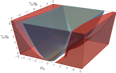
For concreteness, we show in Fig. 2 stability diagrams of a probe immersed in an odd incompressible viscoelastic fluid. Figures 2(a), 2(c) and 2(d) display the unstable (red) regions of the parameter space and the passive (blue) regions, where the thermodynamics constraint (7) is satisfied. These two regions are disjoint, as expected from thermodynamics. Note that the three-dimensional view of the parameter space $(\nu_{\rm o},\gamma_{\rm o}\eta_{\rm s},\gamma_{\rm s}\eta_{\rm s})$ of Fig. 2(d) shows the symmetry $(\nu_{\rm o},\gamma_{\rm o})\to(-\nu_{\rm o},-\gamma_{\rm o})$ of the system.

As the intuition would suggest, the friction $\gamma_{\rm s}$, which characterizes the elastic stress relaxation, has a stabilizing role and increasing it always leads to more stable systems. On the other hand, the odd coupling $\nu_{\rm o}$ is destabilizing the system as its magnitude is increased (provided its sign is kept constant). The odd elastic relaxation term $\gamma_{\rm o}$ has a more subtle effect and may have a destabilizing or stabilizing influence [see Fig. 2(a)].

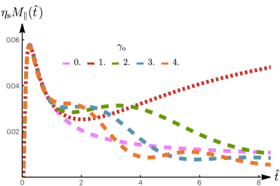
Figure 2(b) highlights the consequences of the odd active coefficients on the time-dependent (drag) response $M_{\parallel}(t)$ experienced by the particle along its velocity. In the linearly stable regions [points $A$ and $B$ in panel 2(a)], the drag decays to 0, indicating that the initial perturbation is eventually damped by viscous friction. On the other hand, the parallel response corresponding to parameters in the active unstable region [point $C$ in panel 2(a)] increases with time, indicating that the probe motion is accelerated by the active fluid surrounding it. This acceleration must eventually be compensated by nonlinearities that we have not considered in the present analysis.

(a)

(b)

(c)

(d)

Figure 3: Drag response $\eta_{\rm s}M_{\parallel}$ of an odd incompressible viscoelastic fluid as a function of the dimensionless time $\hat{t}=t/\tau_{0}$ with $\tau_{0}=a^{2}\rho_{0}/\eta_{\rm s}$. (a) In the absence of the odd elastic stress relaxation ($\gamma_{\rm o}=0$) and for different values of $\nu_{\rm o}$. (b) In the presence of an odd elastic stress relaxation ($\gamma_{\rm o}\eta_{\rm s}=8$) and for different values of $\nu_{\rm o}$. (c) Drag response for a varied odd elastic stress relaxation $\gamma_{\rm o}$ and a vanishing $\nu_{\rm o}$. (d) Drag response for a varied odd elastic stress relaxation $\gamma_{\rm o}$ and $\nu_{\rm o}=-1.2$. In all panels, the solid lines indicate passive fluids for which Eq. (7) is satisfied, while dashed lines are used for active fluids. The red lines with small dashing are unstable active drag responses for which Eq. (20) is violated. Such responses diverge at long time and nonlinear mechanisms should be included to obtain the corresponding large-time behavior. Other parameters are: $\nu_{\rm s}=1$, $\gamma_{\rm s}\eta_{\rm s}=0.3$, $G_{\rm s}\tau_{0}/\eta_{\rm s}=0.25$.

Broken Onsager symmetry. We now continue the discussion in the case of an incompressible fluid with broken Onsager symmetry, that is, $\bm{\nu}^{\prime}\neq\bm{\nu}$. We define $\nu^{\prime}_{\rm s,o}=c_{\rm s,o}+e_{\rm s,o}$ and $\nu_{\rm s,o}=c_{\rm s,o}-e_{\rm s,o}$, such that the Onsager symmetry is recovered for $e_{\rm s,o}=0$. Breaking Onsager symmetry modifies the conditions for stability, although these new conditions take a form similar to those given in Eq. (20). They read (we simplified the notation by taking $c_{\rm s,o}=\nu_{\rm s,o}$):

$$e_{\rm o}^{2}-e_{\rm s}^{2}+4\gamma_{\rm s}\eta_{\rm s}-\nu_{\rm o}^{2}+\nu_{\rm s}^{2}>0,$$ (21a)

$$2\eta_{\rm s}\gamma_{\rm o}^{2}+2\gamma_{\rm o}\nu_{\rm o}\nu_{\rm s}+\gamma_{\rm s}\!\left(2\gamma_{\rm s}\eta_{\rm s}-\nu_{\rm o}^{2}+\nu_{\rm s}^{2}\right)+\gamma_{-}>0,$$ (21b)

and

$$\Delta\!<\!0\,\,\text{or}\,\begin{cases}\Delta\geq 0\,\quad\text{and}\\ \gamma_{\rm s}\!\left(\nu_{\rm s}^{2}-\nu_{\rm o}^{2}\right)\!-\!2\gamma_{\rm o}\nu_{\rm o}\nu_{\rm s}\!+\!8\eta_{\rm s}\gamma_{\rm s}^{2}\!+\!\gamma_{+}\!\!<\!0\end{cases}\!\!\!$$ (21c)

with $\gamma_{\pm}=\gamma_{\rm s}(e_{\rm o}^{2}-e_{\rm s}^{2})\pm 2\gamma_{\rm o}e_{\rm s}e_{\rm o}$ and $\Delta=b_{1}^{2}-4b_{0}b_{2}$, where $b_{0}=4G_{\rm s}^{3}\gamma_{\rm s}(\gamma_{\rm s}^{2}+\gamma_{\rm o}^{2})$, $b_{1}=G_{\rm s}^{2}[\gamma_{\rm s}(8\gamma_{\rm s}\eta_{\rm s}-\nu_{\rm o}^{2}+\nu_{\rm s}^{2})-2\gamma_{\rm o}\nu_{\rm o}\nu_{\rm s}+\gamma_{+}]/(\tau_{0}\eta_{\rm s})$, $b_{2}=G_{\rm s}(e_{\rm o}^{2}-e_{\rm s}^{2}+4\gamma_{\rm s}\eta_{\rm s}-\nu_{\rm o}^{2}+\nu_{\rm s}^{2})/(\tau_{0}^{2}\eta_{\rm s})$.

Importantly, note that $e_{\rm o}$ alone cannot destabilize the system, which is consistent with this coefficient entering anti-symmetrically the entropy production rate. In fact, taking $e_{\rm s}=0$ in Eq. (21) shows that the constraints are more easily satisfied for $e_{\rm o}\neq 0$ and $e_{\rm o}$ even has a stabilizing effect.

On the other hand, a non-vanishing $e_{\rm s}$ can drive the system into an unstable regime, even if the thermodynamic constraint $2\eta_{\rm s}\gamma_{\rm s}\geq\nu_{\rm o}^{2}$ is satisfied. If $e_{\rm s}\neq 0$ and $\gamma_{\rm o}\neq 0$, the odd deviation from Onsager symmetry $e_{\rm o}$ can also play a role in destabilizing the system through the term $\gamma_{\rm o}e_{\rm s}e_{\rm o}$ entering Eq. (21).

III Drag and lift response

III.1 Drag response for an incompressible fluid

In this Section we consider the response along the velocity direction [drag, $M_{\rm\parallel}(s)$] and perpendicular to it [lift, $M_{\rm\perp}(s)$], making the decomposition

$$\mathbb{M}_{ij}(s)=M_{\rm\parallel}(s)\delta_{ij}-M_{\rm\perp}(s)\varepsilon_{ij}\,.$$ (22)

For simplicity, we enforce Onsager symmetry in this Section and take $\bm{\nu}^{\prime}=\bm{\nu}$. We first consider the incompressible limit, so that $M_{\rm\perp}^{\rm inc}(s)=0$, whereas the drag response coefficient reads:

$$M_{\rm\parallel}^{\rm inc}(s)=\frac{1}{4\pi A_{\rm s}(s)}K_{0}\left(\sqrt{\frac{s\tau_{0}}{A_{\rm s}(s)/\eta_{\rm s}}}\right)\,,$$ (23)

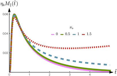
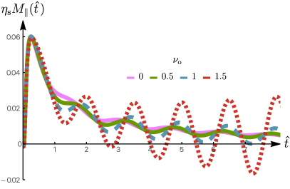
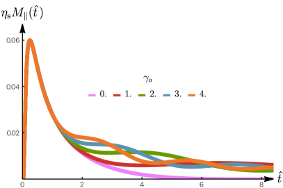
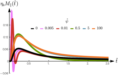
with $\tau_{0}=\rho_{0}a^{2}/\eta_{\rm s}$ and $K_{0}(z)$ the $0^{\rm th}$ modified Bessel function of the second kind. The corresponding drag response in time domain can be obtained numerically (see App. F for details), and the results are displayed in Fig. 3. In Figs. 3(a) and 3(b), we explore the role of the odd elastic strain relaxation rate $\gamma_{\rm o}$.

A nonvanishing $\gamma_{\rm o}$ [Fig. 3(b)] leads to a long-lived oscillatory behavior, despite strain relaxation due to plasticity. This is a unique property that can signal odd viscoelasticity in experiment. Furthermore, we note that the amplitude of these oscillations are strongly amplified by the odd elasticity coefficient $\nu_{\rm o}$. It highlights the nontrivial interplay between these different terms, that was already observed in Sec. II.2 for the stability constrains. It shows that increasing $\gamma_{\rm o}$ and $\nu_{\rm o}$ cannot be increased indefinitely without inducing instabilities. Specifically, the dashed line in Fig. 3(a) (corresponding to $\nu_{\rm o}\geq\gamma_{\rm s}^{2}+\nu_{\rm s}^{2}$) corresponds to a diverging trajectory. Such a non-converging drag response should be regularized by nonlinear corrections.

In Figs. 3(c) and 3(d), we compute the drag response for a varied $\gamma_{\rm o}$ for $\nu_{\rm o}=0$ and $\nu_{\rm o}=1$, respectively. We find that an increasing $\gamma_{\rm o}$ leads to an increasing oscillation frequency. In Fig. 3(d), the choice of $\nu_{\rm o}$ makes the viscoelastic fluid active, and it was shown in Sec. II.2 that this may induce instabilities for the motion of the probe particle. This is the case for the dashed line, which violates the stability constraint of Eq. (20b).

III.2 Drag and lift response for a compressible fluid

(a)

(b)

Figure 4: Drag and lift responses of an odd compressible viscoelastic fluid induced as a function of the dimensionless time $\hat{t}=t/\tau_{0}$ with $\tau_{0}=a^{2}\rho_{0}/\eta_{\rm s}$. (a) Drag response $\eta_{\rm s}M_{\parallel}$ for different values of the dimensionless inverse compressibility $\hat{\psi}=\psi\eta_{\rm s}^{2}/(a\rho_{0})^{2}$. (b) Lift response $\eta_{\rm s}M_{\perp}$ for different values of the dimensionless inverse compressibility $\hat{\psi}$. Other parameters are: $\nu_{\rm s}=\nu_{\rm b}=1$, $\gamma_{\rm s}\eta_{\rm s}=1$, $G_{\rm s}\tau_{0}/\eta_{\rm s}=1$, $\eta_{\rm b}/\eta_{\rm s}=0$, $\gamma_{\rm b}\eta_{\rm s}=0$, $G_{\rm b}\tau_{0}/\eta_{\rm s}=0$, $\eta_{\rm o}/\eta_{\rm s}=0.1$, $\gamma_{\rm o}\eta_{\rm s}=0.1$, $\nu_{\rm o}=0$.

Compressibility is a necessary condition for observing lift forces, a signature of odd fluids. In this Section, we thus discuss how a finite compressibility of the fluid can be considered within our framework. Although exploring systematically the role of finite compressibility for the response of a probe in an odd viscoelastic medium is beyond the scope of this paper, we illustrate here a few important features of finite compressibility.

To relax the incompressibility constraint while continuing analytic computations, we consider a weak oddity approximation, i.e. we consider $\eta_{\rm o},\gamma_{\rm o}$ and $\nu_{\rm o}$ small compared to their shear and bulk counterparts. We introduce $\varepsilon_{\rm o}$ the corresponding small parameter (for instance, $\varepsilon_{\rm o}=\eta_{\rm o}/\eta_{\rm s}$). We discuss here the first nonvanishing correction, although the series expansion can be continued to higher orders. Starting from Eq. (15), we obtain the response coefficients that were defined in Eq. (22):

$$M_{\rm\parallel}(s) =M_{\rm\parallel}^{\rm inc}(s)+\frac{\Theta(s)K_{0}\left(\sqrt{\tau_{0}s\Theta(s)}\right)}{4\pi\eta_{\rm s}}+\mathcal{O}(\varepsilon_{\rm o}^{2})\,,$$ (24a)

$$\begin{split}M_{\rm\perp}(s)&=\frac{\tau_{0}sA_{\rm o}(s)/\eta_{\rm s}}{\hat{\psi}^{-1}+\tau_{0}sA_{\rm b}(s)/\eta_{\rm s}}\Bigg{[}2M_{\rm\parallel}^{\rm inc}(s)\\ &-\frac{\Theta(s)K_{0}\left(\sqrt{\tau_{0}s\Theta(s)}\right)}{2\pi\eta_{\rm s}}\Bigg{]}+\mathcal{O}(\varepsilon_{\rm o}^{2})\,,\end{split}$$ (24b)

where we have defined the dimensionless compressibility $$\hat{\psi}=\psi\eta_{\rm s}^{2}/(a\rho_{0})^{2}$$ and

$$\Theta(s)=\frac{\tau_{0}s}{\hat{\psi}^{-1}+\tau_{0}s\left(A_{\rm b}(s)+A_{\rm s}(s)\right)/\eta_{\rm s}}\,.$$ (24c)

As expected, the lift response vanishes in the incompressible limit $\hat{\psi}\to 0$. Note also the absence of odd corrections to the drag response [Eq. (24a)] at first order.

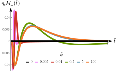
Figure 4 displays the drag and lift responses for different values of $\hat{\psi}$, illustrating the role of a finite compressibility. Increasing the compressibility $\hat{\psi}$ spreads out the response in time both for the drag and lift coefficients. For small values of the compressibility, we observe a short-time response, eventually converging to the incompressible limit [black line with empty circles, Fig. 4(a)]. The lift response, which is a hallmark of odd systems and thus vanishes in the absence of the odd coefficients, is shown in Fig. 4(b). Note the rapid sign change of the lift coefficient, which becomes more pronounced and symmetrical as the compressibility $\hat{\psi}$ is decreased, leading eventually to a vanishing lift response in the incompressible limit $\hat{\psi}\to 0$.

IV Discussion

In this work, we considered the stability of two-dimensional odd viscoelastic fluids by looking at the motion of probe particles that experience a push at $t=0$. We considered contributions to the constitutive equation that are allowed for passive systems (as found in Ref. Lier et al. (2022)), as well as active terms that rely on fuel consumption at a microscopic level. Such active terms modify the passive picture by breaking the two hallmarks of passive hydrodynamics: Onsager-symmetry and positive-definiteness of the Onsager matrices. To characterize the effect of activity, we first discussed the stability condition of a probe in a generic, compressible odd viscoelastic fluid, before focusing on the incompressible limit, where the discussion is simpler while the essential ingredients are kept. Importantly, although lift force vanishes Abanov et al. (2018) in this limit, odd viscoelastic effects manifest themselves spectacularly as they can destabilize the probe motion. We find that passive odd viscoelastic fluids, where viscoelastic coefficients are constrained by the Second Law of Thermodynamics, are always linearly stable. We find the converse statement that active odd viscoelastic fluids are always unstable not to be true. Specifically, we find that there is an intermediate region where the motion of probe particles is stable, despite the system being active and constantly consuming fuel. In this intermediate regime, there is a non-trivial interplay between the odd elasticity coefficient $\nu_{\rm o}$ and odd plasticity $\gamma_{\rm o}$, which is graphically displayed in Fig. 2. This interplay is even more surprising considering that odd plasticity is a non-dissipative phenomenon and therefore plays no role in determining the passivity of an odd viscoelastic fluid Lier et al. (2022). Similarly, the non-dissipative shear elastic coefficient $\nu_{\rm s}$ is involved in stability constraints despite being non-dissipative.

The stability of viscoelastic models was considered in previous works by looking at the stability of perturbative modes. In Ref. Lier et al. (2022), a small wave-vector analysis yielded a constraint identical to Eq. (20b), which is one of the three constraints obtained in this work for stable probe particle motion that are given in Eq. (20). In Ref. Floyd et al. (2022), odd viscoelastic materials were studied in the context of the formation of spatial-temporal patterns, whose presence indicate instability. The authors performed a numerical analysis of the perturbative modes to determine their stability for a range of wave vectors. The numerical findings of Ref. Floyd et al. (2022), showing that odd elasticity can destabilize the viscoelastic material, whereas shear elasticity, plasticity and viscosity tend to stabilize the viscoelastic material qualitatively agree with the analytic constraints derived in the present work. Such a qualitative finding is also consistent with the analytically derived stability constraint of Eq. (20b) found in Ref. Lier et al. (2022).

In this work, we furthermore considered the effect of several odd viscoelastic coefficients on probe particle motion. The obtained results provide a viscoelastic extension of Ref. Ganeshan and Abanov (2017) for the incompressible case and of Refs. Hosaka et al. (2021b); Lier et al. (2023) for the compressible case, which considered lift and drag force for an odd viscous fluid. When generalizing to viscoelastic fluids, one must consider inhomogeneities in time to see qualitatively different effects, as at vanishing frequencies only viscous effects remain. For this reason, we only considered the motion of a probe particle after a push at $t=0$. A computational advantage of doing so is that there is no problem arising from the Stokes paradox Veysey and Goldenfeld (2007), which for the steady case was resolved in Refs. Hosaka et al. (2021b); Lier et al. (2023) by regularizing the integral with momentum relaxation coming from the three-dimensional bulk. We first considered the incompressible limit, which is a limit that is decoupled from passivity constraints and therefore a useful limit for considering active destabilizing effects. One key qualitative feature that we find is that the relaxing velocity becomes oscillatory for a non-zero odd plasticity coefficient $\gamma_{\rm o}$ and that the amplitude of this oscillation is amplified by the odd elasticity coefficient $\nu_{\rm o}$. This again highlights the non-trivial interplay between these two odd viscoelastic coefficients, and is illustrated in Fig. 3. Lastly, we discussed the role of compressibility in the response of the probe. In this case, we showed that the odd lift force, transverse to the direction of motion of the probe particle, that exists for viscous odd fluids, becomes time-dependent in viscoelastic systems. We discussed this case focusing on a small oddity limit, where analytical results can be obtained, and the results are displayed in Fig. 4. In the compressible regime, probes placed in a linearly unstable odd viscoelastic fluid are likely to perform limit cycles in the plane. Exploring these limit cycles, and more generally the probe motion in the linearly-unstable regime is an interesting aspect which requires introducing nonlinear terms whose symmetry and time-dependence need to be discussed. We leave this work for future publications.

Acknowledgements.— The authors wish to acknowledge Debarghya Banerjee, Gwynn Elfring, Alexander Morozov and Tzer Han Tan for inspiring discussions. C.D. acknowledges the support of the LabEx “Who Am I?” (ANR-11-LABX-0071) and of the Université Paris Cité IdEx (ANR-18-IDEX-0001) funded by the French Government through its “Investments for the Future” program. PS was supported by the DFG through the Leibniz Program and the cluster of excellence ct.qmat (EXC 2147, project-id 39085490) and the National Science Centre (NCN) Sonata Bis grant 2019/34/E/ST3/00405.

Appendix A Constitutive equations for active odd materials

In this Appendix, we will derive the most general constitutive equations for the conserved currents by constraining entries using the Onsager relations and the Second Law of Thermodynamics. In Sec. A.1, we first consider the passive case, following to a large extent the steps performed in Ref. Callan-Jones and Jülicher (2011). This analysis will yield a result that coincides with Ref. Lier et al. (2022) where a general model for passive odd viscoelasticity was constructed. Then we consider the active case in Sec. A.2. Here, like in Ref. Jülicher et al. (2018), we add fuel consumption, which allows for a much broader class of non-equilibrium corrections, for which we consider the effect of some of them on the motion of beads in the main text.

A.1 Passive chiral viscoelastic fluid

In order to hydrodynamically describe a viscoelastic fluid we first formulate the conservation laws in absence of external forces and torques. Firstly, there is conservation of mass density $\rho$ and momentum $g_{i}$

$$\partial_{t}\rho+\partial_{i}(\rho v_{i}) =0~{}~{},$$ (25a)

$$\partial_{t}g_{i}-\partial_{j}\sigma^{\rm tot}_{ij} =0~{}~{},$$ (25b)

where $$\sigma^{\rm tot}_{ij} v_{i} g_{i}=\rho v_{i}$$ is the total stress, is the fluid velocity. Momentum is related to fluid velocity as . In addition, we have conservation of angular momentum, given by

$$\partial_{t}l_{ij}+\partial_{k}M_{ijk} =-2\sigma^{\rm tot}_{[ij]}~{}~{},$$ (25c)

$l_{ij}$ the density of intrinsic angular momentum and $M_{ijk}$ is the angular momentum flux. Another property that is important for describing the state of viscoelastic fluids the object $u_{ij}$. In the elastic limit, $u_{ij}$ is the elastic strain, however for general viscoelastic fluids $u_{ij}$ can undergo relaxation through plastic deformations Fukuma and Sakatani (2011); Azeyanagi et al. (2009). To study the evolution of $u_{ij}$ and the behavior the viscoelastic fluid in general, we start with formulating a local free energy Jülicher et al. (2018); Callan-Jones and Jülicher (2011):

$$\mathcal{F}=\int\left(\frac{1}{2}\rho v^{2}+f(u_{ij})\right)\differential V\,,$$ (26)

where $f(u_{ij})$ the local free energy density, which depends on $u_{ij}$. $u_{ij}$ is conjugate to the local elastic stress $\sigma^{\rm el}_{ij}$, such that $\sigma^{\rm el}_{ij}=\partial f/\partial u_{ij}$. For an isotropic solid, the local free energy density at leading order in strain is given by

$$f(u_{ij})=f_{0}+G_{\rm s}(\tilde{u}_{ij})^{2}+\frac{1}{2}G_{\rm b}(u_{jj})^{2}\,.$$ (27)

To derive the constitutive equations for the viscoelastic fluid using the standard hydrodynamic approach, we decompose our stress into

$$\sigma^{\rm tot}_{ij}=-\rho v_{i}v_{j}-P\delta_{ij}+\sigma_{ij}\,,$$ (28)

where $\sigma_{ij}$ is the deviatoric stress. The deviatoric stress is the part of the stress that incorporates the corrections to a perfect fluid corresponding to a theory of local thermal equilibrium. The pressure $P$ is obtained with the Euler relation

$$P=-f+\mu n~{}~{},$$ (29)

with $\mu$ being the chemical potential and where the density $n$ is given by $n=\rho/m$. If one considers the change of time of $F$, one finds upon plugging in the conservation laws of Eq. (25) that the entropy production rate $\Theta$ is given by Jülicher et al. (2018); Callan-Jones and Jülicher (2011)

$$T\Theta=\sigma_{ij}v_{ij}-\frac{{\rm D}u_{ij}}{{\rm D}t}\sigma^{\rm el}_{ij}+\frac{1}{2}\partial_{k}\omega_{ij}M_{ijk}\,,$$ (30)

where we introduced the rotation $\omega_{ij}=\partial_{i}v_{j}-\partial_{j}v_{i}$ as well as the corotational derivative which for a general two-tensor $a_{ij}$ is given by

$$\frac{{\rm D}a_{ij}}{{\rm D}t}=\partial_{t}a_{ij}+v_{k}\partial_{k}a_{ij}+\omega_{ik}a_{kj}+\omega_{jk}a_{ik}~{}~{}.$$ (31)

Because of the conservation of angular momentum given by Eq. (25c), there is no contribution coming from the anti-symmetric stress in the entropy production rate of Eq. (30) Salbreux and Jülicher (2017). Instead, there is only a contribution from the deviatoric angular momentum flux $M_{ijk}$, which will give contributions to the equations of motion that are two orders higher in gradients, and these contributions will therefore be omitted. Note that because odd viscoelastic fluids are often introduced by chiral agents that draw arbitrary amounts of angular momentum from the environment, the conservation of angular momentum tends not to hold. In the absence of angular momentum conservation, there are ways in which the anti-symmetric stress can get hydrodynamic corrections. However, we will omit these anti-symmetric contributions for simplicity by upholding angular momentum conservation. Having the entropy production rate of Eq. (30) at our disposal, we are now ready to construct the Onsager matrix with containing the most general entries in the deviatoric currents. An important difference compared to the isotropic achiral viscoelastic fluids in two dimensions is that, in addition to the identity, the fully anti-symmetric two-dimensional Levi-Civita tensor $\varepsilon_{ij}$ can be used to construct entries in the constitutive equations. As we will discuss below, these tensors can feature components that are odd under the exchange of indices. This can for example give rise to odd viscosity Avron et al. (1995); Lévay (1995); Jensen et al. (2012); Soni et al. (2019). Such terms signal parity-breaking, and for passive two-dimensional systems, one often finds that this breaking of parity is accompanied by a breaking of time-reversal symmetry, as is for example the case for parity-breaking induced by a background magnetic field. We therefore uphold symmetry under the simultaneous transformation of parity and time-reversal when deriving the passive constitutive equations, which modify the Onsager relations. The details of this are provided in App. C. From the expression of entropy production (30) and the Onsager relations, we obtain the following constitutive relations:

$$\sigma_{ij} =2\eta^{\rm p}_{\rm s}\tilde{v}_{ij}+\eta^{\rm p}_{\rm b}v_{kk}\delta_{ij}+2\eta^{\rm p}_{\rm o}v^{\rm o}_{ij}+\nu^{\rm p}_{\rm s}\sigma^{\rm el}_{ij}+\frac{1}{2}\nu^{\rm p}_{\rm b}\sigma^{\rm el}_{kk}\delta_{ij}+\nu^{\rm p}_{\rm o}(\sigma^{\rm el})^{\rm o}_{ij}\,,$$ (32a)

$$\frac{{\rm D}u_{ij}}{{\rm D}t} =-\gamma^{\rm p}_{\rm s}\tilde{\sigma}^{\rm el}_{ij}-\frac{1}{2}\gamma^{\rm p}_{\rm b}\sigma^{\rm el}_{kk}\delta_{ij}-\gamma^{\rm p}_{\rm o}(\sigma^{\rm el})^{\rm o}_{ij}+\nu^{\rm p}_{\rm s}v_{ij}+\frac{1}{2}\nu^{\rm p}_{\rm s}v_{kk}\delta_{ij}+\nu^{\rm p}_{\rm o}{v}^{\rm o}_{ij}\,.$$ (32b)

What we see in Eq. (32) are the shear, bulk and odd viscosity given by the $\eta$-terms, as well as $\gamma$-terms representing shear and bulk plasticity, as well as a coefficient that could be called “odd plasticity”. This odd plasticity was first considered in Ref. Son (2019). Then, there are $\nu$-terms which are non-equilibrium corrections representing shear, bulk and odd elasticity, the latter of which was first considered as an active term in Ref. Scheibner et al. (2020). Using the compact notation described in App. B, Eq. (32) can be rewritten as

$$\underline{\underline{\sigma}} =\bm{\nu}^{\rm p}:\underline{\underline{\sigma}}^{\rm el}+2\bm{\eta}^{\rm p}:\underline{\underline{v}}\,,$$ (33a)

$$\frac{{\rm D}\underline{\underline{u}}}{{\rm D}t} =-\bm{\gamma}^{\rm p}:\underline{\underline{\sigma}}^{\rm el}+\bm{\nu}^{\rm p}:\underline{\underline{v}}\,.$$ (33b)

To see the dissipative properties of the entries in the constitutive equations of Eq. (33), we plug Eq. (32) back into Eq. (30), which yields

$$T\Theta={\rm Tr}\left[2\eta^{\rm p}_{\rm s}\tilde{\underline{\underline{v}}}\cdot\tilde{\underline{\underline{v}}}+2\nu^{\rm p}_{\rm o}\left(\tilde{\underline{\underline{\sigma}}}^{\rm el}\cdot\underline{\underline{\varepsilon}}\cdot\tilde{\underline{\underline{v}}}\right)+\gamma^{\rm p}_{\rm s}\tilde{\underline{\underline{\sigma}}}^{\rm el}\cdot\tilde{\underline{\underline{\sigma}}}^{\rm el}\right]+2\eta_{\rm b}^{\rm p}\Tr[v]^{2}+\gamma_{\rm b}^{\rm p}\Tr[v]^{2}~{}~{}.$$ (34)

Requiring the first term on the right hand side of Eq. (34) to be non-negative is equivalent to requiring that the matrix

$$\begin{pmatrix}2\eta^{\rm p}_{\rm s}\underline{\underline{\mathbbm{1}}}&-\nu^{\rm p}_{\rm o}\underline{\underline{\varepsilon}}\\ \nu^{\rm p}_{\rm o}\underline{\underline{\varepsilon}}&\gamma^{\rm p}_{\rm s}\underline{\underline{\mathbbm{1}}}\end{pmatrix}$$ (35)

is semi-definite positive, which is satisfied if all its eigenvalues have non-negative real part. As was found in Ref. Lier et al. (2022), this condition is guaranteed if, in addition to $\eta^{\rm p}_{\rm s},\gamma^{\rm p}_{\rm s},\eta^{\rm p}_{\rm b},\gamma^{\rm p}_{\rm b}\geq 0$, we have

$$2\eta^{\rm p}_{\rm s}\gamma^{\rm p}_{\rm s}\geq\left(\nu^{\rm p}_{\rm o}\right)^{2}~{}~{},$$ (36)

which is the thermodynamic constraint given in Eq. (6).

A.2 Active chiral viscoelastic fluid

The passive model we have introduced above can be generalized by considering activity induced by microscopic fuel consumption of microscopic agents Jülicher et al. (2018). The rate of fuel consumption can be represented $\Delta\mu$, which is the chemical potential difference of a chemical reaction, multiplied by a scalar reaction rate $r$. Because of this fuel consumption, the entropy production rate of Eq. (30) is generalized to

$$T\Theta=\sigma_{ij}v_{ij}-\frac{{\rm D}u_{ij}}{{\rm D}t}\sigma^{\rm el}_{ij}+\frac{1}{2}\partial_{k}\omega_{ij}M_{ijk}+r\Delta\mu~{}~{},$$ (37)

This new contribution opens up a wide range of new possible entries in the constitutive equations, which are given by

$$\underline{\underline{\sigma}} =\bm{\nu}^{\rm p}:\underline{\underline{\sigma}}^{\rm el}+2\bm{\eta}^{\rm p}:\underline{\underline{v}}+\Delta\mu\left(\bm{\zeta}^{(1)}:\underline{\underline{\sigma}}^{\rm el}+2\bm{\zeta}^{(2)}:\underline{\underline{v}}\right)\,,$$ (38a)

$$\frac{{\rm D}\underline{\underline{u}}}{{\rm D}t} =-\bm{\gamma}^{\rm p}:\underline{\underline{\sigma}}^{\rm el}+\bm{\nu}^{\rm p}:\underline{\underline{v}}+\Delta\mu\left(-\bm{\zeta}^{(3)}:\underline{\underline{\sigma}}^{\rm el}+\bm{\zeta}^{(4)}:\underline{\underline{v}}\right)\,.$$ (38b)

The active terms ($\propto\Delta\mu$) can be absorbed into a redefinition of the parameters so that constitutive equations read:

$$\underline{\underline{\sigma}} =\bm{\nu}:\underline{\underline{\sigma}}^{\rm el}+2\bm{\eta}:\underline{\underline{v}}\,,$$ (39a)

$$\frac{{\rm D}\underline{\underline{u}}}{{\rm D}t} =-\bm{\gamma}:\underline{\underline{\sigma}}^{\rm el}+\bm{\nu}^{\prime}:\underline{\underline{v}}\,,$$ (39b)

which is Eq. (4) in the main text. The new parameters are related to the passive ones of Eq. (38) by $\bm{\eta}=\bm{\eta}^{\rm p}+\Delta\mu\bm{\zeta}^{(2)}$, $\bm{\gamma}=\bm{\gamma}^{\rm p}+\Delta\mu\bm{\zeta}^{(3)}$, $\bm{\nu}=\bm{\nu}^{\rm p}+\Delta\mu\bm{\zeta}^{(1)}$ and $\bm{\nu}^{\prime}=\bm{\nu}^{\rm p}+\Delta\mu\bm{\zeta}^{(4)}$. Note that $\Delta\mu$, as can be seen in Eq. (37), is a thermodynamic force Jülicher et al. (2018) corresponding to the flux $r$. Because $\Delta\mu$ is a thermodynamic force, it should be a small correction with respect to the local equilibrium. This means that the $\Delta\mu\underline{\underline{\sigma}}^{\rm el}$- and $\Delta\mu\underline{\underline{v}}$-terms are second order, and one would therefore naively think that these terms should be neglected. However, these second-order terms play an important qualitative role as the effective coefficients appearing in $\bm{\eta},\bm{\gamma},\bm{\nu},\bm{\nu}^{\prime}$ are not bound by the passivity constraint (36). In particular, this allows for the presence of active odd elasticity.

To make sure that the second law constraint $\Theta\geq 0$ in Eq. (37) as well as the Onsager relations described in App. C are satisfied, we require the corresponding reaction rate to be

$$r =\Lambda\Delta\mu+\Tr[-\underline{\underline{\sigma}}^{\rm el}:\bm{\zeta}^{(1)}:\underline{\underline{v}}+2\underline{\underline{v}}:\bm{\zeta}^{(2)}:\underline{\underline{v}}+\underline{\underline{\sigma}}^{\rm el}:\bm{\zeta}^{(3)}:\underline{\underline{\sigma}}^{\rm el}+\underline{\underline{v}}:\bm{\zeta}^{(4)}:\underline{\underline{\sigma}}^{\rm el}]~{}~{}.$$ (40)

Appendix B Compact tensor notation and odd isotropic rank-4 tensor algebra

In this Appendix, we describe the notation used for describing tensors and their contractions. First, we describe vectors and two-tensors with a single and a double underline, i.e.

$$V_{i}\rightarrow\underline{V}~{}~{},~{}~{}T_{ij}\rightarrow\underline{\underline{T}}~{}~{}.$$ (41)

We define the components of an odd isotropic rank-4 tensor $\bm{B}$ in the following way:

$$B_{ijkl}=\frac{B_{\rm s}}{2}\left(\delta_{ik}\delta_{jl}+\delta_{il}\delta_{jk}-\delta_{ij}\delta_{kl}\right)+\frac{B_{\rm b}}{2}\delta_{ij}\delta_{kl}+\frac{B_{\rm o}}{4}\left(\delta_{ik}\varepsilon_{jl}+\delta_{il}\varepsilon_{jk}+\delta_{jk}\varepsilon_{il}+\delta_{jl}\varepsilon_{ik}\right)\,.$$ (42)

These tensors are symmetric with respect to their first two and last two indices, such that $B_{ijkl}=B_{jikl}$ and $B_{ijkl}=B_{ijlk}$. The contraction of an odd isotropic rank-4 tensor $\bm{B}$ with an arbitrary rank-2 tensor $\underline{\underline{b}}$ reads:

$$(\bm{B}:\underline{\underline{b}})_{ij}=B_{ijkl}b_{kl}=B_{\rm s}\tilde{b}_{ij}+\frac{B_{\rm b}}{2}{\rm Tr}(b)\delta_{ij}+B_{\rm o}\tilde{b}^{\rm o}_{ij}\,,$$ (43)

where

$${\rm Tr}(b) =b_{jj}\,,\quad\tilde{b}_{ij}=\frac{1}{2}\left(b_{ij}+b_{ji}\right)-\frac{1}{2}b_{kk}\delta_{ij}\,,\quad\tilde{b}^{\rm o}_{ij}=\varepsilon_{ik}\tilde{b}_{kj}\,.$$ (44)

One important relation that is used in App. A is

$$\underline{\underline{a}}:\bm{A}:\underline{\underline{a}}=A_{\rm s}(\tilde{a}_{ij})^{2}+\frac{1}{2}A_{\rm b}({\rm Tr}(a))^{2}~{}~{},$$ (45)

where we see that the odd contribution drops out due to its anti-symmetric nature. Consistently with the definition (43), we define the contraction $\bm{C}=\bm{A}:\bm{B}$ of two tensors $\bm{A}$ and $\bm{B}$ in terms of their components as:

$$C_{ijkl}=A_{ijmn}B_{mnkl}\,.$$ (46)

Odd isotropic rank-4 tensors form a commutative group under multiplication since

$$C_{ijkl}=A_{ijmn}B_{mnkl}=\frac{C_{\rm s}}{2}\left(\delta_{ik}\delta_{jl}+\delta_{il}\delta_{jk}-\delta_{ij}\delta_{kl}\right)+\frac{C_{\rm b}}{2}\delta_{ij}\delta_{kl}+\frac{C_{\rm o}}{4}\left(\delta_{ik}\varepsilon_{jl}+\delta_{il}\varepsilon_{jk}+\delta_{jk}\varepsilon_{il}+\delta_{jl}\varepsilon_{ik}\right)\,,$$ (47)

where

$$C_{\rm s}=A_{\rm s}B_{\rm s}-A_{\rm o}B_{\rm o}\,,\quad C_{\rm b}=A_{\rm b}B_{\rm b}\,,\quad C_{\rm o}=A_{\rm o}B_{\rm s}+A_{\rm s}B_{\rm o}\,,$$ (48)

where we have used the relation $\varepsilon_{ij}\varepsilon_{kl}=\delta_{ik}\delta_{jl}-\delta_{il}\delta_{jk}$. The identity tensor $\bm{I}$ is defined component-wise as:

$$I_{ijkl}=\frac{1}{2}\left(\delta_{ik}\delta_{jl}+\delta_{il}\delta_{jk}\right)\,,$$ (49)

and the inverse $\bm{N}=\bm{M}^{-1}$ of $\bm{M}$ satisfies $\bm{M}^{-1}\bm{M}=\bm{M}\bm{M}^{-1}=\bm{I}$ and has the following elements:

$$N_{\rm s}=\frac{M_{\rm s}}{M_{\rm s}^{2}+M_{\rm o}^{2}}\,,\quad N_{\rm b}=\frac{1}{M_{\rm b}}\,,\quad N_{\rm o}=-\frac{M_{\rm o}}{M_{\rm s}^{2}+M_{\rm o}^{2}}\,.$$ (50)

Appendix C Onsager relations with odd isotropic rank-4 tensors

In this appendix, we derive Onsager relations in the case where the state variables $\underline{\underline{\Phi}}^{\alpha}$ of the system are rank-2 symmetric tensors. We define their conjugate forces as $\underline{\underline{f}}^{\alpha}=-\delta\mathcal{F}/\delta\underline{\underline{\Phi}}^{\alpha}$ where $\mathcal{F}[\underline{\underline{\Phi}}]$ is the free energy of the system. The time derivative of the free energy can therefore be written as:

$$\dot{\mathcal{F}}=-\sum_{\alpha}\dot{\Phi}_{ij}^{\alpha}f_{ij}^{\alpha}\,,$$ (51)

where the summation over repeated Latin indices is implicit, while we write explicitly the summation over Greek indices. Considering linear relations between thermodynamics fluxes and forces read:

$$\dot{\underline{\underline{\Phi}}}^{\alpha}=\sum_{\beta}\bm{{\cal L}}^{\alpha\beta}:\underline{\underline{f}}^{\beta}\,,$$ (52)

where each $\bm{\mathcal{L}}^{\alpha\beta}$ is an odd isotropic rank-4 tensor. Writing explicitly the components, we have:

$$\dot{\Phi}_{ij}^{\alpha}=\sum_{\beta}{\cal L}_{ijkl}^{\alpha\beta}f_{kl}^{\beta}\,,$$ (53)

We deduce:

$$\dot{\mathcal{F}}=-\sum_{\alpha\beta}(\bm{{\cal L}}^{\alpha\beta}:\underline{\underline{f}}^{\beta})_{ij}f_{ij}^{\alpha}=-\sum_{\alpha\beta}{\cal L}_{ijkl}^{\alpha\beta}f_{ij}^{\alpha}f_{kl}^{\beta}\,,$$ (54)

from which we deduce that the odd part of the diagonal elements of $\bm{{\cal L}}$ (i.e. the coefficients ${\cal L}^{\alpha\alpha}_{\rm o}$) do not contribute to the rate of change of the free energy as a consequence of Eq. (45). We now derive the symmetries of the Onsager matrix $\bm{\mathcal{L}}^{\alpha\beta}$ under time reversal. For this purpose, we first introduce the partition function:

$$\mathcal{Z}=\int{\cal D}\underline{\underline{\Phi}}\,{\rm e}^{-\mathcal{F}[\underline{\underline{\Phi}}]/k_{B}T}\,,$$ (55)

that can be used to compute correlation functions. We have:

$$\begin{split}\langle\underline{\underline{\Phi}}^{\alpha}\underline{\underline{f}}^{\beta}\rangle&=\frac{1}{\mathcal{Z}}\int{\cal D}\underline{\underline{\Phi}}\,\underline{\underline{\Phi}}^{\alpha}\underline{\underline{f}}^{\beta}{\rm e}^{-\mathcal{F}[\underline{\underline{\Phi}}]/k_{B}T}\,,\\ &=-\frac{1}{\mathcal{Z}}\int{\cal D}\underline{\underline{\Phi}}\,\underline{\underline{\Phi}}^{\alpha}\frac{\delta F}{\delta\underline{\underline{\Phi}}^{\beta}}{\rm e}^{-\mathcal{F}[\underline{\underline{\Phi}}]/k_{B}T}\,,\\ &=\frac{k_{B}T}{\mathcal{Z}}\int{\cal D}\underline{\underline{\Phi}}\,\underline{\underline{\Phi}}^{\alpha}\frac{\delta}{\delta\underline{\underline{\Phi}}^{\beta}}{\rm e}^{-\mathcal{F}[\underline{\underline{\Phi}}]/k_{B}T}\,,\\ &=-\frac{k_{B}T}{\mathcal{Z}}\int{\cal D}\underline{\underline{\Phi}}\frac{\delta\underline{\underline{\Phi}}^{\alpha}}{\delta\underline{\underline{\Phi}}^{\beta}}{\rm e}^{-\mathcal{F}[\underline{\underline{\Phi}}]/k_{B}T}\,,\\ &=-k_{B}T\delta^{\alpha\beta}\bm{I}\,.\end{split}$$ (56)

Note that the same procedure can be used to obtain relations for higher order correlations functions. Considering for simplicity scalar quantities, we have the generic expression:

$$\langle\phi^{\alpha_{1}}\cdots\phi^{\alpha_{N}}f^{\beta}\rangle=-k_{B}T\left(\delta^{\alpha_{1}\beta}\langle\phi^{\alpha_{2}}\cdots\phi^{\alpha_{N}}\rangle+\delta^{\alpha_{2}\beta}\langle\phi^{\alpha_{1}}\phi^{\alpha_{3}}\cdots\phi^{\alpha_{N}}\rangle+\cdots\right)\,.$$ (57)

The last equality of Eq. (56) is best derived using indices:

$$\frac{\delta\Phi_{ij}^{\alpha}}{\delta\Phi_{kl}^{\beta}}=\frac{1}{2}\left(\delta_{ik}\delta_{jl}+\delta_{il}\delta_{jk}\right)\delta^{\alpha\beta}=I_{ijkl}\delta^{\alpha\beta}\,,$$ (58)

where we have used the fact that the $\underline{\underline{\Phi}}^{\alpha}$ are symmetric tensors. The second to last equality in Eq. (56) has been obtained using an integration by parts. The boundary terms vanish with the assumption that $F$ diverges at infinity. Using Eqs. (53) and (56) , we can now compute:

$$\begin{split}\langle\Phi_{ij}^{\alpha}\dot{\Phi}_{kl}^{\beta}\rangle&=\langle\Phi_{ij}^{\alpha}{\cal L}_{klmn}^{\beta\gamma}f_{mn}^{\gamma}\rangle\,,\\ &={\cal L}_{klmn}^{\beta\gamma}\langle\Phi_{ij}^{\alpha}f_{mn}^{\gamma}\rangle\,,\\ &=-k_{B}T{\cal L}_{klij}^{\beta\alpha}\,.\end{split}$$ (59)

The same correlation function can also be computed using time reversal. We have:

$$\begin{split}\langle\underline{\underline{\Phi}}^{\alpha}\dot{\underline{\underline{\Phi}}}^{\beta}\rangle&=\underset{\Delta t\to 0}{{\rm lim}}\frac{1}{\Delta t}\left(\langle\underline{\underline{\Phi}}^{\alpha}(t)\underline{\underline{\Phi}}^{\beta}(t+\Delta t)\rangle-\langle\underline{\underline{\Phi}}^{\alpha}(t)\underline{\underline{\Phi}}^{\beta}(t)\rangle\right)\,,\\ &=\underset{\Delta t\to 0}{{\rm lim}}\frac{1}{\Delta t}\left(\langle\underline{\underline{\Phi}}^{\alpha}(t-\Delta t)\underline{\underline{\Phi}}^{\beta}(t)\rangle-\langle\underline{\underline{\Phi}}^{\alpha}(t)\underline{\underline{\Phi}}^{\beta}(t)\rangle\right)\,,\\ &=\underset{\Delta t\to 0}{{\rm lim}}\frac{\epsilon^{\alpha}\epsilon^{\beta}}{\Delta t}\left(\overline{\langle\underline{\underline{\Phi}}^{\alpha}(-t+\Delta t)\underline{\underline{\Phi}}^{\beta}(-t)\rangle}-\overline{\langle\underline{\underline{\Phi}}^{\alpha}(-t)\underline{\underline{\Phi}}^{\beta}(-t)\rangle}\right)\,,\\ &=\underset{\Delta t\to 0}{{\rm lim}}\frac{\epsilon^{\alpha}\epsilon^{\beta}}{\Delta t}\left(\overline{\langle\underline{\underline{\Phi}}^{\alpha}(t+\Delta t)\underline{\underline{\Phi}}^{\beta}(t)\rangle}-\overline{\langle\underline{\underline{\Phi}}^{\alpha}(t)\underline{\underline{\Phi}}^{\beta}(t)\rangle}\right)\,,\\ &=\epsilon^{\alpha}\epsilon^{\beta}\overline{\langle\dot{\underline{\underline{\Phi}}}^{\alpha}\underline{\underline{\Phi}}^{\beta}\rangle}\,,\end{split}$$ (60)

where $\epsilon^{\alpha}$ is the signature of $\underline{\underline{\Phi}}^{\alpha}$ under time reversal and the overline $\overline{\cdots}$ indicates that the sign of some parameters (for instance magnetic field) has to be changed. We thus deduce the Onsager matrix symmetry:

$${\cal L}_{ijkl}^{\alpha\beta}=\epsilon^{\alpha}\epsilon^{\beta}\overline{{\cal L}}_{klij}^{\beta\alpha}\,.$$ (61)

It yields in particular:

$${\cal L}_{ijkl}^{\alpha\alpha}=\overline{{\cal L}}_{klij}^{\alpha\alpha}\,,$$ (62)

which means that an equilibrium odd viscosity needs to change sign under time reversal to be non-vanishing. This is consistent for instance with odd viscosity Avron et al. (1995); Lévay (1995); Jensen et al. (2012); Soni et al. (2019), which is proportional to the magnetic field and therefore changes sign upon time reversal. Assuming a sign change upon time-reversal for all odd coefficients thus leads to the following structure for the Onsager matrix:

$$\bm{{\cal L}}^{\alpha\beta}=\begin{pmatrix}\bm{\eta}^{\rm p}&-\bm{\nu}^{\rm p}\\ \bm{\nu}^{\rm p}&\bm{\gamma}^{\rm p}\end{pmatrix}^{\alpha\beta}\,,$$ (63)

where $\bm{\eta}^{\rm p}$, $\bm{\nu}^{\rm p}$ and $\bm{\gamma}^{\rm p}$ are isotropic rank-4 tensors that include odd and even parts. This yields Eq. (33).

Appendix D Shell localization

In this Appendix, we explain how shell localization is used to obtain the response matrix of Eq. (16). For this, we first invert Eq. (14) as

$$v_{i}(\mathbf{k},s)=\mathcal{G}^{-1}_{ij}(\mathbf{k},s)f^{\text{ext}}_{j}(\mathbf{k},s)~{}~{}.$$ (64)

Eq. (64) gives the velocity induced by a force for a given Fourier wave vector and Laplace frequency. We then consider the force applied on a probe particle, which is a rigid disk of radius $a$ located at the origin. Due to the rotational symmetry of the disk, we can decompose the force density as

$$f^{\text{ext}}_{j}(s,\mathbf{k})=L(k)F_{j}(s)~{}~{}.$$ (65)

The shell localization method amounts to assuming that the force density is uniformly localized our the surface of the probe particle Levine and Lubensky (2001); Camley and Brown (2011); MacKintosh and Lubensky (1991), i.e.

$$L(\mathbf{x})=\frac{1}{2\pi a}\delta(|\mathbf{x}|-a)\,.$$ (66)

The assumption of a uniform distribution in real space has been found to give consistent results for systems where no-slip boundary conditions apply Levine and Lubensky (2001); Weisenborn and Mazur (1984); Lier et al. (2023). Fourier transforming Eq. (66) yields

$$L(k)=J_{0}(ak)~{}~{},$$ (67)

with $J_{0}(z)$ the $0^{\rm th}$ Bessel function of the first kind. To obtain the bead velocity, we must inverse Fourier transform Eq. (64) to obtain the fluid velocity in real space which is coupled to the probe particle velocity through no-slip boundary conditions. The most accurate way to do this would to relate the probe particle velocity $U_{i}(s)$ to $v_{i}(|\mathbf{x}|=a,s)$, which can be done averaging over the boundary line between the fluid and the probe particle Weisenborn and Mazur (1984). We instead consider the fluid velocity localized at $|\mathbf{x}|=0$, i.e. we relate

$$U_{i}(s)=v_{i}(|\mathbf{x}|=0,s)~{}~{},$$ (68)

as has also been done in Refs. Camley and Brown (2011); Levine and Lubensky (2001); Lier et al. (2023). As shown in Ref. Weisenborn and Mazur (1984), averaging over velocities at $|x|=a$ would yield an additional factor $J_{0}(ak)$ in the integrand of Eq. (16). However, this modification only leads to minor quantitative effects, and we thus ignore it for mathematical simplicity.

Appendix E Computing the probe particle stability for active odd fluids

E.1 General case

In this Appendix, we detail the stability analysis of a probe particle in an active odd viscoelastic fluid, as discussed in Sec. II. Such stability is determined by the long-term velocity of the probe particle. This velocity follows from Eq. (12), which can be rewritten as

$$U_{i}(t) =\frac{1}{2{\rm i}\pi}\int_{\Gamma-{\rm i}\infty}^{\Gamma+{\rm i}\infty}\!\!{\rm d}s\,{\rm e}^{st}\int\frac{{\rm d}^{2}\mathbf{k}}{(2\pi)^{2}}\mathcal{M}_{ij}(\mathbf{k},s)L(k)F_{j}(s)\,,$$ (69)

where $\Gamma$ is a real number so that the contour path of integration is in the region of convergence of the integrand. As discussed in the main text, we consider a force perturbation along the eigendirections of $\mathcal{M}_{ij}$, and furthermore consider an instantaneous perturbation applied at $t=0$, such that $F_{j}(t)\propto\delta(t)$, or $F_{j}(s)\propto 1$ in Laplace space. The velocity of the probe after this initial perturbation is thus given by:

$$U_{i}(t) =\frac{1}{2{\rm i}\pi}\int_{\Gamma-{\rm i}\infty}^{\Gamma+{\rm i}\infty}\!\!{\rm d}s\,{\rm e}^{st}\int\frac{{\rm d}^{2}\mathbf{k}}{(2\pi)^{2}}m_{i}(\mathbf{k},s)L(k)\,,$$ (70)

where $m_{i}(\mathbf{k},s)$ depends on the eigenvalues of $\mathcal{M}_{ij}$ and on the form of the initial perturbation. We will not focus on its precise expression in the following discussion, but the crucial point is that $m_{i}(\mathbf{k},s)$ is a rational fraction in $s$. This implies that the inverse Laplace transform can be computed as:

$$U_{i}(t) =\sum_{\ell}\int\frac{{\rm d}^{2}\mathbf{k}}{(2\pi)^{2}}\,m_{i,\ell}(\mathbf{k})L(k)\,{\rm e}^{s_{\ell}^{*}(\mathbf{k})t}\,,$$ (71)

where the $s_{\ell}^{*}(\mathbf{k})$ are the poles in $s$ of the rational fraction $m_{i}$ and where the $m_{i,\ell}(\mathbf{k})$ are the residues of $m_{i}$ at $s=s_{\ell}^{*}(\mathbf{k})$. As a consequence of this simple form, a sufficient condition for the long-time stability of the probe is directly given by the sign of the real part of the poles of $m_{i}$:

$${\rm Re}\left(s_{\ell}^{*}(\mathbf{k})\right)\leq 0\qquad\forall\ell,\,\forall\mathbf{k}\,,$$ (72)

which is the condition given in the main text.

E.2 Incompressible limit

To continue our analysis while keeping the technicalities to a minimum, we now restrict to the incompressible case. In this simpler case, $\mathcal{M}_{ij}$ is proportional to the identity tensor, such that the probe velocity can be written as:

$$U_{i}(t) =\frac{1}{2{\rm i}\pi}\int_{\Gamma-{\rm i}\infty}^{\Gamma+{\rm i}\infty}\!\!{\rm d}s\,{\rm e}^{st}\int_{0}^{\infty}\frac{{\rm d}k}{2\pi}r(k,s)F_{i}(s)\,,$$ (73)

where we have defined

$$r(k,s)=\frac{1}{4\pi\eta_{\rm s}}\frac{akJ_{0}(ak)}{\tau_{0}s+(ak)^{2}A_{\rm s}(s)/\eta_{\rm s}}\,,$$ (74)

with $\tau_{0}=\rho_{0}a^{2}/\eta_{\rm s}$, and we only consider instantaneous perturbations ($F_{i}(s)$ constant). As discussed in the previous section, the long-time stability is then given by the poles in $s$ of $r$. They correspond to the roots of the third-order polynomial $P(s)=s^{3}+a_{2}s^{2}+a_{1}s+a_{0}$ with

$$\begin{split}&a_{2}=(ak)^{2}/\tau_{0}+4\gamma_{\rm s}G_{\rm s}\,,\\ &a_{1}=G_{\rm s}\left[4G_{\rm s}(\gamma_{\rm o}^{2}+\gamma_{\rm s}^{2})+\frac{(ak)^{2}}{\tau_{0}\eta_{\rm s}}\left(4\gamma_{\rm s}\eta_{\rm s}-\nu_{\rm o}^{2}+\nu_{\rm s}^{2}\right)\right]\,,\\ &a_{0}=\frac{2G_{\rm s}^{2}(ak)^{2}}{\tau_{0}\eta_{\rm s}}\left[2\eta_{\rm s}\gamma_{\rm o}^{2}+2\gamma_{\rm o}\nu_{\rm o}\nu_{\rm s}+\gamma_{\rm s}\left(2\gamma_{\rm s}\eta_{\rm s}-\nu_{\rm o}^{2}+\nu_{\rm s}^{2}\right)\right]\,,\end{split}$$ (75)

where we have considered the case $\nu_{\rm s,o}^{\prime}=\nu_{\rm s,o}$. The roots $s_{\ell}^{*}(k)$ of $P(s)$ all have negative real parts iff $a_{0,1,2}>0$ and $a_{2}a_{1}-a_{0}>0$ according to the Routh–Hurwitz stability criterion. We note that $a_{2}$ is always positive. The conditions $a_{0,1}>0$ are equivalent to:

$$4\gamma_{\rm s}\eta_{\rm s}-\nu_{\rm o}^{2}+\nu_{\rm s}^{2}>0\,,\quad$$ (76a)

$$2\eta_{\rm s}\gamma_{\rm o}^{2}+2\gamma_{\rm o}\nu_{\rm o}\nu_{\rm s}+\gamma_{\rm s}\left(2\gamma_{\rm s}\eta_{\rm s}-\nu_{\rm o}^{2}+\nu_{\rm s}^{2}\right)>0\,.\quad$$ (76b)

The condition $$a_{2}a_{1}-a_{0}>0 Q(X)=b_{2}X^{2}+b_{1}X+b_{0} X=(ak)^{2} b_{0}=8G_{\rm s}^{3}\gamma_{\rm s}(\gamma_{\rm s}^{2}+\gamma_{\rm o}^{2}) b_{1}=G_{\rm s}^{2}[\gamma_{\rm s}(8\gamma_{\rm s}\eta_{\rm s}-\nu_{\rm o}^{2}+\nu_{\rm s}^{2})-2\gamma_{\rm o}\nu_{\rm o}\nu_{\rm s}]/(\tau_{0}\eta_{\rm s}) b_{2}=G_{\rm s}(4\gamma_{\rm s}\eta_{\rm s}-\nu_{\rm o}^{2}+\nu_{\rm s}^{2})/(2\tau_{0}^{2}\eta_{\rm s}) \Delta=b_{1}^{2}-4b_{0}b_{2} Q a_{2}a_{1}-a_{0}>0$$ takes the form of a second-order polynomial with and , , . With the discriminant of , the condition thus translates to:

$$\Delta<0\,\,\text{or}\,\begin{cases}\Delta\geq 0\,\quad\text{and}\\ \gamma_{\rm s}\left(\nu_{\rm s}^{2}-\nu_{\rm o}^{2}\right)-2\gamma_{\rm o}\nu_{\rm o}\nu_{\rm s}+8\eta_{\rm s}\gamma_{\rm s}^{2}<0\end{cases}\!\!\!.$$ (76c)

A similar analysis can be conducted for $\nu_{\rm s,o}^{\prime}\neq\nu_{\rm s,o}$.

Appendix F Inverse Laplace transform in the incompressible case

(a)

Figure 5: Contour integration in the complex plane used to compute the inverse Laplace transform (79). The dashed blue lines along the real axis indicate branch cuts of the integrand. In order to compute the integrals $G_{i}$ along the contours $\mathcal{C}_{i}$, the radius of the large circle $R$ and the width $2\varepsilon$ between the segments above and below the real axis are sent to $\infty$ and $0$, respectively.

In this Appendix we compute explicitly the velocity of a probe immersed in an odd incompressible visco-elastic fluid. In the incompressible limit, the probe velocity $U_{i}(t)$ is directly obtained as the inverse Laplace transform of the complex velocity $U_{i}(s)$:

$$U_{i}(t)=\frac{1}{2{\rm i}\pi}\int_{\Gamma-{\rm i}\infty}^{\Gamma+{\rm i}\infty}\!\!{\rm d}s\,{\rm e}^{st}U_{i}(s)\,,$$ (77a)

where $$U_{i}(s)$$ was obtained in Eq. (23) and we rewrite it here for convenience:

$$U_{i}(s)=\frac{K_{0}\left(\sqrt{\frac{s\tau_{0}}{A_{\rm s}(s)/\eta_{\rm s}}}\right)}{4\pi A_{\rm s}(s)}F_{i}(s)\,.$$ (77b)

As we will see in the following, the computation of the inverse Laplace transform requires performing contour integration in the complex plane which have to be carefully designed due to the presence of the square root in Eq. (77b). Therefore, in order to simplify the following discussion, we consider the case where the coefficient $\gamma_{\rm o}$ vanishes, although a similar result can be obtained in the general case. For $\gamma_{\rm o}=0$, the complex viscosity $A_{\rm s}$ reads:

$$A_{\rm s}(s)=\eta_{\rm s}\frac{s-s_{1}}{s-s_{2}}\,,$$ (78)

where $s_{1}=-G_{\rm s}(2\eta_{\rm s}\gamma_{\rm s}-\nu_{\rm o}^{2}+\nu_{\rm s}^{2})/\eta_{\rm s}$ and $s_{2}=-2\gamma_{\rm s}G_{\rm s}$. Note that $s_{2}<0$ while $s_{1}$ can be either sign, and is positive in the unstable regime according to Eq. (20b). In the following, we consider the unstable case and have $s_{2}<0<s_{1}$. We also introduce $\Delta s=s_{2}-s_{1}<0$ for convenience. The computation in the stable case ($s_{1}<0$) follows the same steps.

Finally, we consider the velocity after an instantaneous force is applied. We thus take $F_{j}(t)\propto\delta(t)$ (or $F_{j}(s)\propto 1$ in Laplace space) and the drag response defined in Eq. (22) reads:

$$\eta_{\rm s}M_{\parallel}(t)=\frac{1}{4\pi}\int_{\Gamma-{\rm i}\infty}^{\Gamma+{\rm i}\infty}\!\!\frac{{\rm d}s}{2{\rm i}\pi}\,g(s){\rm e}^{st}\,,\quad g(s)=\frac{s-s_{2}}{s-s_{1}}K_{0}\left(\sqrt{\frac{s(s-s_{2})}{s-s_{1}}}\right)\,,$$ (79)

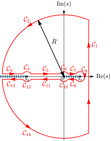
This inverse Laplace transform can be computed using residues. We first note that the function $g(s)$ has branch cuts for ${\rm Re}\left[s(s-s_{2})/(s-s_{1})\right]<0$, that is for ${\rm Re}(s)<s_{2}$ and $0<{\rm Re}(s)<s_{1}$, and is analytic otherwise. We thus define a closed integration contour (see Fig. 5) that avoids the branch cuts and such that $\sum_{i}G_{i}=0$ where $G_{i}=\int_{\mathcal{C}_{i}}{\rm d}s\,g(s){\rm e}^{st}/(2{\rm i}\pi)$. In the following, we detail the computation of the $G_{i>1}$.

Contours $\mathcal{C}_{2}$ and $\mathcal{C}_{14}$. We set $s=R{\rm e}^{{\rm i}\theta}$ with $\theta\in[\pi/2,\pi]$ such that:

$$G_{2}=\lim_{R\to\infty}\frac{1}{2{\rm i}\pi}\int_{\pi/2}^{\pi}{\rm d}\theta\,{\rm i}R{\rm e}^{{\rm i}\theta}\frac{R{\rm e}^{{\rm i}\theta}-s_{2}}{R{\rm e}^{{\rm i}\theta}-s_{1}}K_{0}\left(\sqrt{R}{\rm e}^{{\rm i}\theta/2}\sqrt{\frac{R{\rm e}^{{\rm i}\theta}-s_{2}}{R{\rm e}^{{\rm i}\theta}-s_{1}}}\right){\rm e}^{R{\rm e}^{{\rm i}\theta}t}\,,$$ (80)

which vanishes in the limit $R\to\infty$ because of the last exponential factor in the above equation with real part $Rt\cos\theta\leq 0$ (for $t>0$ and $\theta\in[\pi/2,\pi]$). Similarly, we find $G_{14}=0$.

Contours $\mathcal{C}_{3}$ and $\mathcal{C}_{13}$. For $\mathcal{C}_{3}$, we set $s=s_{2}+{\rm e}^{{\rm i}\pi}u$ with $u\in[0,\infty[$, from which we obtain:

$$G_{3} =\frac{1}{2{\rm i}\pi}\int_{\infty}^{0}{\rm d}u\,{\rm e}^{{\rm i}\pi}\frac{{\rm e}^{{\rm i}\pi}u}{{\rm e}^{{\rm i}\pi}u+s_{2}-s_{1}}K_{0}\left(\sqrt{\frac{({\rm e}^{{\rm i}\pi}u+s_{2}){\rm e}^{{\rm i}\pi}u}{{\rm e}^{{\rm i}\pi}u+s_{2}-s_{1}}}\right){\rm e}^{(s_{2}+{\rm e}^{{\rm i}\pi}u)t}\,,$$ (81)

$$=\frac{1}{2{\rm i}\pi}\int_{0}^{\infty}{\rm d}u\,\frac{u}{u-\Delta s}K_{0}\left({\rm i}\sqrt{u}\sqrt{\frac{(u-s_{2})}{u-\Delta s}}\right){\rm e}^{s_{2}t}{\rm e}^{-ut}\,.$$ (82)

Similarly, setting $s=s_{2}+{\rm e}^{-{\rm i}\pi}u$ along $\mathcal{C}_{13}$ yields:

$$G_{13} =-\frac{1}{2{\rm i}\pi}\int_{0}^{\infty}{\rm d}u\,\frac{u}{u-\Delta s}K_{0}\left(-{\rm i}\sqrt{u}\sqrt{\frac{(u-s_{2})}{u-\Delta s}}\right){\rm e}^{s_{2}t}{\rm e}^{-ut}\,.$$ (83)

Contours $\mathcal{C}_{4}$ and $\mathcal{C}_{12}$. For $\mathcal{C}_{4}$, we set $s=s_{2}+\varepsilon{\rm e}^{{\rm i}\phi}$ with $\phi\in[0,\pi]$, from which we obtain:

$$G_{4} =\lim_{\varepsilon\to 0}\frac{1}{2{\rm i}\pi}\int_{\pi}^{0}{\rm d}\phi\,\varepsilon{\rm i}{\rm e}^{{\rm i}\phi}\frac{\varepsilon{\rm e}^{{\rm i}\phi}}{\varepsilon{\rm e}^{{\rm i}\phi}+\Delta s}K_{0}\left(\sqrt{\varepsilon}{\rm e}^{{\rm i}\phi/2}\sqrt{\frac{{\rm e}^{{\rm i}\pi}\varepsilon+s_{2}}{{\rm e}^{{\rm i}\pi}\varepsilon-s_{1}}}\right){\rm e}^{(s_{2}+\varepsilon{\rm e}^{{\rm i}\phi})t}\,,$$ (84)

$$=\lim_{\varepsilon\to 0}\frac{1}{2{\rm i}\pi}\int_{\pi}^{0}{\rm d}\phi\,\frac{\varepsilon^{2}}{\Delta s}K_{0}\left(\sqrt{\varepsilon}{\rm e}^{{\rm i}\phi/2}\sqrt{\frac{s_{2}}{-s_{1}}}\right){\rm e}^{s_{2}t}\,,$$ (85)

which vanishes in the limit $\varepsilon\to 0$ since $K_{0}(x)\underset{{x\to 0}}{\sim}-\log x$. Similar steps yield $G_{12}=0$.

Contours $\mathcal{C}_{5}$ and $\mathcal{C}_{11}$. The contributions stemming from $\mathcal{C}_{4}$ and $\mathcal{C}_{11}$ cancel each other, since they correspond to an integration in both direction of a holomorphic function along these contours.

Contours $\mathcal{C}_{6}$ and $\mathcal{C}_{10}$. For $\mathcal{C}_{6}$, we set $s=\varepsilon{\rm e}^{{\rm i}\phi}$ with $\phi\in[0,\pi]$, from which a computation similar of that of $G_{4}$ yields:

$$G_{5} =\lim_{\varepsilon\to 0}\frac{1}{2{\rm i}\pi}\int_{\pi}^{0}{\rm d}\phi\,\frac{s_{2}}{s_{1}}\varepsilon K_{0}\left(\sqrt{\varepsilon}{\rm e}^{{\rm i}\phi/2}\sqrt{\frac{s_{2}}{s_{1}}}\right)\,,$$ (86)

which vanishes in the limit $\varepsilon\to 0$. Similar steps yield $G_{10}=0$.

Contours $\mathcal{C}_{7}$ and $\mathcal{C}_{9}$. For $\mathcal{C}_{7}$, we set $s=s_{1}+s_{1}u{\rm e}^{{\rm i}\pi}$ with $v\in[0,1]$, from which we obtain:

$$G_{7} =\frac{1}{2{\rm i}\pi}\int_{0}^{1}{\rm d}v\,\frac{\Delta s+s_{1}v}{v}K_{0}\left({\rm e}^{-{\rm i}\pi/2}\sqrt{\frac{(v-1)(s_{1}v+\Delta s)}{v}}\right){\rm e}^{s_{1}(1-v)t}\,.$$ (87)

Similarly, setting $s=s_{2}+{\rm e}^{-{\rm i}\pi}u$ along $\mathcal{C}_{13}$ yields:

$$G_{9} =-\frac{1}{2{\rm i}\pi}\int_{0}^{1}{\rm d}v\,\frac{\Delta s+s_{1}v}{v}K_{0}\left({\rm e}^{+{\rm i}\pi/2}\sqrt{\frac{(v-1)(s_{1}v+\Delta s)}{v}}\right){\rm e}^{s_{1}(1-v)t}\,.$$ (88)

Contour $\mathcal{C}_{8}$. We set $s=s_{1}+\varepsilon{\rm e}^{{\rm i}\phi}$ with $\phi\in[-\pi,\pi]$, from which we obtain:

$$G_{8} =\lim_{\varepsilon\to 0}\frac{1}{2{\rm i}\pi}\int_{\pi}^{-\pi}{\rm d}\phi\,(-\Delta s)K_{0}\left(\frac{1}{\sqrt{\varepsilon}}{\rm e}^{{\rm i}\phi/2}\sqrt{s_{1}(-\Delta s)}\right){\rm e}^{s_{1}t}\,,$$ (89)

which vanishes in the limit $\varepsilon\to 0$ since $K_{0}(x)\underset{{x\to\infty}}{\sim}-\sqrt{\pi/(2x)}\,{\rm e}^{-x}$.

Since $\eta_{\rm s}M_{\parallel}(t)=G_{1}/(4\pi)$ and $G_{1}=-\sum_{i>1}G_{i}=-(G_{3}+G_{13}+G_{7}+G_{9})$, we finally obtain:

$$\eta_{\rm s}M_{\parallel}(t)=\frac{1}{8\pi}\left[\int_{0}^{\infty}{\rm d}u\,a(u,t)+\int_{0}^{1}{\rm d}v\,b(v,t)\right]\,,$$ (90a)

with

$$a(u,t) =\frac{u}{u-\Delta s}J_{0}\left(\sqrt{\frac{u(u-s_{2})}{u-\Delta s}}\right){\rm e}^{s_{2}t-ut}\,,$$ (90b)

$$b(v,t) =\frac{\Delta s+s_{1}v}{-v}J_{0}\left(\sqrt{\frac{(v-1)(s_{1}v+\Delta s)}{v}}\right){\rm e}^{s_{1}(1-v)t}\,,$$ (90c)

and where we have used the identities $K_{0}({\rm i}x)-K_{0}(-{\rm i}x)=-{\rm i}\pi J_{0}(x)$ for $x>0$. Importantly, we verify that in the long-time limit the behavior of $M_{\parallel}(t)\underset{{t\to\infty}}{\sim}{\rm e}^{s_{1}t}$ is set by the real part of $s_{1}$ (since $(s_{2}-u)t$ is always negative), and thus diverges, as expected for our choice $s_{1}>0$.

References

- Epstein and Mandadapu (2020) J. M. Epstein and K. K. Mandadapu, “Time-reversal symmetry breaking in two-dimensional nonequilibrium viscous fluids,” Phys. Rev. E 101, 052614 (2020).
- Hargus et al. (2020) C. Hargus, K. Klymko, J. M. Epstein, and K. K. Mandadapu, “Time reversal symmetry breaking and odd viscosity in active fluids: Green–Kubo and NEMD results,” J. Chem. Phys. 152, 201102 (2020).
- Lier et al. (2022) R. Lier, J. Armas, S. Bo, C. Duclut, F. Jülicher, and P. Surówka, “Passive odd viscoelasticity,” Phys. Rev. E 105, 054607 (2022).
- Han et al. (2021) M. Han, M. Fruchart, C. Scheibner, S. Vaikuntanathan, J. J. de Pablo, and V. Vitelli, “Fluctuating hydrodynamics of chiral active fluids,” Nat. Phys. 17, 1260 (2021).
- Hargus et al. (2021) C. Hargus, J. M. Epstein, and K. K. Mandadapu, “Odd Diffusivity of Chiral Random Motion,” Phys. Rev. Lett. 127, 178001 (2021).
- Soni et al. (2019) V. Soni, E. S. Bililign, S. Magkiriadou, S. Sacanna, D. Bartolo, M. J. Shelley, and W. T. M. Irvine, “The odd free surface flows of a colloidal chiral fluid,” Nat. Phys. 15, 1188–1194 (2019).
- Reichhardt and Reichhardt (2019) C. Reichhardt and C. J. O. Reichhardt, “Active microrheology, Hall effect, and jamming in chiral fluids,” Phys. Rev. E 100, 012604 (2019).
- Markovich and Lubensky (2021) T. Markovich and T. C. Lubensky, “Odd Viscosity in Active Matter: Microscopic Origin and 3D Effects,” Phys. Rev. Lett. 127, 048001 (2021).
- Reichhardt and Reichhardt (2022) C. J. O. Reichhardt and C. Reichhardt, “Active rheology in odd-viscosity systems,” EPL 137, 66004 (2022).
- Fürthauer et al. (2012) S. Fürthauer, M. Strempel, S. W. Grill, and F. Jülicher, “Active chiral fluids,” Eur. Phys. J. E 35, 89 (2012).
- Tan et al. (2022) T. H. Tan, A. Mietke, J. Li, Y. Chen, H. Higinbotham, P. J. Foster, S. Gokhale, J. Dunkel, and N. Fakhri, “Odd dynamics of living chiral crystals,” Nature 607, 287–293 (2022).
- Banerjee et al. (2021) D. Banerjee, V. Vitelli, F. Jülicher, and P. Surówka, “Active Viscoelasticity of Odd Materials,” Phys. Rev. Lett. 126, 138001 (2021).
- Surówka et al. (2022) P. Surówka, A. Souslov, F. Jülicher, and D. Banerjee, “Odd cosserat elasticity in active materials,” arXiv preprint arXiv:2210.13606 (2022).
- Kalz et al. (2023) E. Kalz, H. D. Vuijk, J.-U. Sommer, R. Metzler, and A. Sharma, “Oscillatory force autocorrelations in equilibrium odd-diffusive systems,” (2023), arXiv:2302.01263 [cond-mat.stat-mech] .
- Kalz et al. (2022) E. Kalz, H. D. Vuijk, I. Abdoli, J.-U. Sommer, H. Löwen, and A. Sharma, “Collisions enhance self-diffusion in odd-diffusive systems,” Phys. Rev. Lett. 129, 090601 (2022).
- Banerjee et al. (2017) D. Banerjee, A. Souslov, A. G. Abanov, and V. Vitelli, “Odd viscosity in chiral active fluids,” Nat. Commun. 8, 1573 (2017).
- Abanov et al. (2018) A. Abanov, T. Can, and S. Ganeshan, “Odd surface waves in two-dimensional incompressible fluids,” SciPost Phys. 5, 010 (2018).
- Ganeshan and Abanov (2017) S. Ganeshan and A. G. Abanov, “Odd viscosity in two-dimensional incompressible fluids,” Phys. Rev. Fluids 2, 094101 (2017).
- Khain et al. (2022) T. Khain, C. Scheibner, M. Fruchart, and V. Vitelli, “Stokes flows in three-dimensional fluids with odd and parity-violating viscosities,” J. Fluid Mech. 934, A23 (2022).
- Hosaka et al. (2023a) Y. Hosaka, R. Golestanian, and A. Daddi-Moussa-Ider, “Hydrodynamics of an odd active surfer in a chiral fluid,” arXiv:2303.11836 (2023a), arxiv:2303.11836 [cond-mat, physics:physics] .
- Hosaka et al. (2021a) Y. Hosaka, S. Komura, and D. Andelman, “Hydrodynamic lift of a two-dimensional liquid domain with odd viscosity,” Phys. Rev. E 104, 064613 (2021a).
- Hosaka et al. (2023b) Y. Hosaka, D. Andelman, and S. Komura, “Pair dynamics of active force dipoles in an odd-viscous fluid,” Eur. Phys. J. E 46, 18 (2023b).
- Scheibner et al. (2020) C. Scheibner, A. Souslov, D. Banerjee, P. Surówka, W. T. M. Irvine, and V. Vitelli, “Odd elasticity,” Nat. Phys. 16, 475 (2020).
- Braverman et al. (2021) L. Braverman, C. Scheibner, B. VanSaders, and V. Vitelli, “Topological Defects in Solids with Odd Elasticity,” Phys. Rev. Lett. 127, 268001 (2021).
- Floyd et al. (2022) C. Floyd, A. R. Dinner, and S. Vaikuntanathan, “Signatures of odd dynamics in viscoelastic systems: From spatiotemporal pattern formation to odd rheology,” arXiv:2210.01159 (2022), arxiv:2210.01159 .
- Fruchart et al. (2022) M. Fruchart, M. Han, C. Scheibner, and V. Vitelli, “The odd ideal gas: Hall viscosity and thermal conductivity from non-Hermitian kinetic theory,” arXiv:2202.02037 (2022), arxiv:2202.02037 .
- Liao et al. (2020) Z. Liao, W. T. M. Irvine, and S. Vaikuntanathan, “Rectification in Nonequilibrium Parity Violating Metamaterials,” Phys. Rev. X 10, 021036 (2020).
- Pellegrino et al. (2017) F. M. D. Pellegrino, I. Torre, and M. Polini, “Nonlocal transport and the Hall viscosity of two-dimensional hydrodynamic electron liquids,” Phys. Rev. B 96, 195401 (2017).
- Narozhny and Schütt (2019) B. N. Narozhny and M. Schütt, “Magnetohydrodynamics in graphene: Shear and Hall viscosities,” Phys. Rev. B 100, 035125 (2019).
- Berdyugin et al. (2019) A. I. Berdyugin, S. G. Xu, F. M. D. Pellegrino, R. Krishna Kumar, A. Principi, I. Torre, M. Ben Shalom, T. Taniguchi, K. Watanabe, I. V. Grigorieva, M. Polini, A. K. Geim, and D. A. Bandurin, “Measuring Hall viscosity of graphene’s electron fluid,” Science 364, 162–165 (2019).
- Fossati et al. (2022) M. Fossati, C. Scheibner, M. Fruchart, and V. Vitelli, “Odd elasticity and topological waves in active surfaces,” arXiv:2210.03669 (2022), arxiv:2210.03669 .
- Green et al. (2020) R. Green, J. Armas, J. de Boer, and L. Giomi, “Topological waves in passive and active fluids on curved surfaces: A unified picture,” arXiv:2011.12271 (2020), arxiv:2011.12271 .
- Souslov et al. (2019) A. Souslov, K. Dasbiswas, M. Fruchart, S. Vaikuntanathan, and V. Vitelli, “Topological Waves in Fluids with Odd Viscosity,” Phys. Rev. Lett. 122, 128001 (2019).
- Tauber et al. (2019) C. Tauber, P. Delplace, and A. Venaille, “A bulk-interface correspondence for equatorial waves,” J. Fluid Mech. 868, R2 (2019).
- Bililign et al. (2022) E. S. Bililign, F. Balboa Usabiaga, Y. A. Ganan, A. Poncet, V. Soni, S. Magkiriadou, M. J. Shelley, D. Bartolo, and W. T. Irvine, “Motile dislocations knead odd crystals into whorls,” Nature Physics 18, 212–218 (2022).
- Mason and Weitz (1995) T. G. Mason and D. A. Weitz, “Optical Measurements of Frequency-Dependent Linear Viscoelastic Moduli of Complex Fluids,” Phys. Rev. Lett. 74, 1250–1253 (1995).
- MacKintosh and Schmidt (1999) F. MacKintosh and C. Schmidt, “Microrheology,” Current opinion in colloid & interface science 4, 300–307 (1999).
- Squires and Mason (2010) T. M. Squires and T. G. Mason, “Fluid Mechanics of Microrheology,” Annu. Rev. Fluid Mech. 42, 413–438 (2010).
- Lier et al. (2023) R. Lier, C. Duclut, S. Bo, J. Armas, F. Jülicher, and P. Surówka, “Lift force in odd compressible fluids,” Phys. Rev. E 108, L023101 (2023).
- Hosaka et al. (2021b) Y. Hosaka, S. Komura, and D. Andelman, “Nonreciprocal response of a two-dimensional fluid with odd viscosity,” Phys. Rev. E 103, 042610 (2021b).
- Gardel et al. (2005) M. Gardel, M. Valentine, and D. Weitz, “Microrheology,” in Microscale Diagnostic Techniques, edited by K. S. Breuer (Springer Berlin Heidelberg, Berlin, Heidelberg, 2005) pp. 1–49.
- Di Leonardo et al. (2010) R. Di Leonardo, L. Angelani, D. Dell’Arciprete, G. Ruocco, V. Iebba, S. Schippa, M. P. Conte, F. Mecarini, F. De Angelis, and E. Di Fabrizio, “Bacterial ratchet motors,” Proceedings of the National Academy of Sciences 107, 9541–9545 (2010).
- Callan-Jones and Jülicher (2011) A. C. Callan-Jones and F. Jülicher, “Hydrodynamics of active permeating gels,” New J. Phys. 13, 093027 (2011).
- Levine and Lubensky (2001) A. J. Levine and T. C. Lubensky, “Response function of a sphere in a viscoelastic two-fluid medium,” Phys. Rev. E 63, 041510 (2001).
- Elfring et al. (2016) G. J. Elfring, L. G. Leal, and T. M. Squires, “Surface viscosity and Marangoni stresses at surfactant laden interfaces,” J. Fluid Mech. 792, 712–739 (2016).
- Stone (1990) H. A. Stone, “A simple derivation of the time-dependent convective-diffusion equation for surfactant transport along a deforming interface,” Physics of Fluids A: Fluid Dynamics 2, 111–112 (1990).
- Weisenborn and Mazur (1984) A. Weisenborn and P. Mazur, “The Oseen drag on a circular cylinder revisited,” Physica A: Statistical Mechanics and its Applications 123, 191–208 (1984).
- Veysey and Goldenfeld (2007) J. Veysey and N. Goldenfeld, “Simple viscous flows: From boundary layers to the renormalization group,” Rev. Mod. Phys. 79, 883–927 (2007).
- Jülicher et al. (2018) F. Jülicher, S. W. Grill, and G. Salbreux, “Hydrodynamic theory of active matter,” Rep. Prog. Phys. 81, 076601 (2018).
- Fukuma and Sakatani (2011) M. Fukuma and Y. Sakatani, “Relativistic viscoelastic fluid mechanics,” Phys. Rev. E 84, 026316 (2011).
- Azeyanagi et al. (2009) T. Azeyanagi, M. Fukuma, H. Kawai, and K. Yoshida, “Universal description of viscoelasticity with foliation preserving diffeomorphisms,” Physics Letters B 681, 290–295 (2009).
- Salbreux and Jülicher (2017) G. Salbreux and F. Jülicher, “Mechanics of active surfaces,” Physical Review E 96, 032404 (2017).
- Avron et al. (1995) J. E. Avron, R. Seiler, and P. G. Zograf, “Viscosity of Quantum Hall Fluids,” Phys. Rev. Lett. 75, 697–700 (1995).
- Lévay (1995) P. Lévay, “Berry phases for Landau Hamiltonians on deformed tori,” J. Math. Phys. 36, 2792–2802 (1995).
- Jensen et al. (2012) K. Jensen, M. Kaminski, P. Kovtun, R. Meyer, A. Ritz, and A. Yarom, “Parity-violating hydrodynamics in 2 + 1 dimensions,” J. High Energ. Phys. 2012, 102 (2012).
- Son (2019) D. T. Son, “Chiral metric hydrodynamics, kelvin circulation theorem, and the fractional quantum hall effect,” (2019).
- Camley and Brown (2011) B. A. Camley and F. L. H. Brown, “Beyond the creeping viscous flow limit for lipid bilayer membranes: Theory of single-particle microrheology, domain flicker spectroscopy, and long-time tails,” Phys. Rev. E 84, 021904 (2011).
- MacKintosh and Lubensky (1991) F. C. MacKintosh and T. C. Lubensky, “Orientational order, topology, and vesicle shapes,” Phys. Rev. Lett. 67, 1169 (1991).