On probing turbulence in core-collapse supernovae in upcoming neutrino detectors

Abstract

Neutrino propagation through a turbulent medium can be highly non-adiabatic leading to distinct signatures in the survival probabilities. A core-collapse supernova can be host to a number of hydrodynamic instabilities which occur behind the shockfront. Such instabilities between the forward shock and a possible reverse shock can lead to cascades introducing turbulence in the associated matter profile, which can imprint itself in the neutrino signal. In this work, we consider realistic matter profiles and seed in the turbulence using a randomization scheme to study its effects on neutrino propagation in an effective two-flavor framework. In particular, we find that the double-dip feature, originally predicted in the neutrino spectra associated with forward and reverse shocks, can be completely washed away in the presence of turbulence, leading to total flavor depolarization. We also study the sensitivity of upcoming neutrino detectors - DUNE and Hyper-Kamiokande- to the power spectrum of turbulence to check for deviations from the usual Kolmogorov ($5/3$) inverse power law. We find that while these experiments can effectively constrain the parameter space for the amplitude of the turbulence power spectra, they will only be mildly sensitive to the spectral index.

I Introduction

The detection of neutrinos from SN1987A can be regarded as one of the first instances of multi-messenger astronomy, where neutrino events were observed hours before visible light. Although limited in statistics - a total of $\mathcal{O}(30)$ neutrino events in the Kamiokande detector [1, 2], the IMB detector [3] and the Baksan detector [4] were observed - this data has been used widely by the particle and astroparticle physics community to probe important questions of fundamental physics.

It is already well-known that neutrinos from a galactic core-collapse supernova (SN) will be our best bet to probe the supernova dynamics. These neutrinos originate from the deepest regions of the SN and propagate through the entire matter envelope before exiting the SN and arriving at the Earth. The flavor composition of the neutrinos is extremely sensitive to the background fermion density it encounters en route. Close to the neutrinosphere, the neutrino density is large enough, so neutrino forward scattering on a neutrino background is the dominant contribution to the propagation Hamiltonian. This can lead to collective flavor conversion - both “slow” [5, 6, 7, 8, 9, 10, 11, 12, 13, 14, 15, 16, 17, 18, 19, 20, 21, 22, 23, 24] and ’‘fast” [25, 26, 27, 28, 29, 25, 26, 27, 30, 31, 32, 31, 33, 34, 35, 36, 37, 38, 39, 40, 41, 42, 43, 44, 45, 46, 47, 48, 49, 50, 51, 52, 53, 54, 55, 56, 57, 58, 59, 60, 61, 32, 62, 63, 64, 65] (see [66, 67, 68, 69] for detailed reviews on the subject)- which is the major mechanism of flavor transformation within radii of $\sim\mathcal{O}(100)\,$km from the neutrinosphere.

At larger radii, neutrino density falls off and matter effects, due to coherent forward scattering on background electrons, become important. Multiple studies have demonstrated the sensitivity of the neutrino spectra to the underlying SN density profile through the Mikheyev-Smirnov-Wolfenstein (MSW) resonances [70, 71], including signatures of the shockwave propagation at late times [72, 73, 74, 75, 76, 77, 78, 79]. In the absence of the shockwave, neutrino propagation is shown to be adiabatic, governed only by the vacuum mixing angle and the matter density. However, violations of adiabaticity can arise due to an abrupt change in density at the shockfront. This non-adiabaticity leaves its imprint on the flavor transition and can be used to reconstruct a real-time propagation of the shockwave.

A distinctive signature of the non-adiabaticity introduced by the shockwave propagation can manifest in the form of dips in the energy-dependent survival probabilities of neutrinos. A few seconds post the SN core bounce, a possible reverse shockwave can arise if a supersonic neutrino-driven wind collides with the ejecta, as shown in Fig. 1. Note that this is very sensitive to whether the neutrino-driven wind is supersonic or subsonic, for a detailed discussion, see [80]. In [77], it was demonstrated that for neutrinos passing through the two density discontinuities, characterised by the reverse and the forward shocks, a “double-dip” feature would be present in the neutrino survival probability as a function of energy. Such a signal can be present in electron neutrinos for normal mass ordering (NMO) and electron antineutrinos for inverted mass ordering (IMO) and can be used to trace the position of the two shockfronts.

However, this is not the complete story. A SN progenitor is host to a variety of hydrodynamic instabilities, which take place behind the shockfront. This leads to turbulence in the ejecta, causing stochastic fluctuations in the matter density. Turbulence is generally expected to be present in aspherical simulations of SNe, and can play an important role in seeding the explosion [81]. These stochastic fluctuations in the matter density have a non-trivial impact on neutrino flavor evolution.

Neutrino flavor evolution in a turbulent medium has been studied extensively to determine its impact on the neutrino spectra from the next Galactic supernova [82, 83, 84, 85, 86, 87, 88, 89, 90, 91]. . Generically, the effect of turbulence on flavor propagation can be broadly classified into two types: (i) ‘stimulated’ or non-adiabatic transitions between different propagation eigenstates if the stochastic density fluctuations are present near the MSW resonance region [84], and (ii) phase effects due to the presence of semi-adiabatic resonances [78]. The latter effect is more subtle and can be suppressed if the amplitude of fluctuations is large.

It is numerically challenging to obtain realistic turbulent matter density profiles from aspherical (3D) hydrodynamic simulations. Theoretically, the effect of turbulence has been modelled by adding disturbances to a smooth matter profile obtained from coarse, spherically symmetric simulations. This can be done in a number of different ways - for example, by adding delta correlated noise [82], or by modelling the turbulent density fluctuations through a Kolmogorov-type power spectrum [83]. In particular, recent 2D hydrodynamic simulations have shown the presence of a power-law dependence of the power spectrum on the wavelength of fluctuations. The long-wavelength fluctuation indeed shows a power-law dependence with the mean spectral index given by $p=1.85^{+0.54}_{-0.77}$, thus indicating that 2D turbulence might be closer to having a Kolmogorov-type power spectrum [85]. However, simulations also indicate that the turbulence might not be fully developed, hence other values of the spectral indices cannot be ruled out. Moreover, it is well known that the cascading of turbulence in 3D is different from 2D [92, 93]. However, the lack of sufficient resolution makes it difficult to recover the Kolmogorov power law behaviour from 3D simulations.

A theoretical study of the impact of turbulence on the neutrino survival probability was performed in [83], where power-law fluctuations in the density profile were assumed. It was found that the electron neutrino survival probability exhibits a power law when the amplitude of turbulence is increased and a corresponding analytical estimate to explain the power law for the simple turbulence model was derived. This was followed by a series of works [88, 89, 90], where the authors used rotating wave approximation to predict the final survival probability amongst other techniques both numerical and analytical. The latter formalism was also used to predict the dependence of the neutrino flavor transition on the amplitude and the spectral index of turbulence. However, various unanswered questions remain. For example, does the “double-dip” feature pointed out in [77] survive in the presence of turbulence? Can turbulence inside a SN media follow a different power-law index than the Kolmogorov prediction, and with what amplitude? Can future-generation neutrino experiments designed to detect thousands of neutrinos from the next galactic supernova actually distinguish between different parameters characterising the turbulence in a supernova?

We aim to shed some light on these questions in this study through a detailed effective two-flavor study of neutrino propagation through a typical SN media profile, characteristic of the cooling phase. We add turbulence to the smooth density profile following the prescription in [86]. We find that the addition of turbulence with an amplitude beyond $10\%$ washes out the double-dip feature completely. We simulate neutrino events in the upcoming DUNE and Hyper-Kamiokande experiment and find that they can distinguish between a turbulent and a non-turbulent SN matter profile with high significance. On the other hand, they do not have enough sensitivity to probe the index of the power spectrum.

Our paper is organized as follows. We discuss turbulence in supernovae and the slab-approximation used as the numerical technique in Sec. II. The algorithm to seed the turbulence along with its impact on neutrino propagation is discussed in Sec. III. The effects of turbulence on the double-dip feature in the neutrino spectra are studied in Sec. III.3. In Sec. IV, we discuss the event rates in DUNE and Hyper-Kamiokande along with their potential to constrain the physical parameters associated with turbulence for a galactic scale supernova. We conclude and discuss the implications of our work in Sec. V. The numerical algorithm developed for this work is summarized in Appendix. A.

II Turbulence in supernovae

We work in the approximate framework of 2-neutrino oscillations, where we have the electron neutrinos ($\nu_{e}$) and $\nu_{x}$ where, $x=\{\mu,\tau\}$, along with each of their antineutrino components. The Equation of Motion (EoM) for a neutrino flavor $|\nu_{\alpha}\rangle$ can be written as

$$\mathrm{i}\frac{d}{dt}|\nu_{\alpha}\rangle=\left[UH_{\rm vac}U^{\dagger}+V(r)\right]|\nu_{\alpha}\rangle\,,$$ (1)

where $H_{\rm vac}={\rm diag}(\Delta m^{2}/(2E),-\Delta m^{2}/(2E))$ is the vacuum Hamiltonian and $U$ is the $2\times 2$ unitary mixing matrix. The matter potential $V(r)$ has a contribution from the forward scattering of neutrinos off the background fermions and is given by $V_{0}(r)=\sqrt{2}G_{F}n_{e}(r){\rm diag}(1,0)$, where $G_{F}$ is the Fermi constant and $n_{e}(r)$ is the electron number density at a given distance $r$. This is extracted from a snapshot of the matter density at a certain time from a simulation. We further neglect the contributions from the non-electron flavor neutrinos, which cancel at the tree-level and arise only at the loop-level [94, 95, 96]. Neutrinos close to the neutrinosphere also experience a forward scattering potential due to their scattering on other background neutrinos [97]. This potential is given by $V_{\nu\nu}\simeq\sqrt{2}G_{F}n_{\nu}$, where $n_{\nu}$ is the total background neutrino density. This neutrino-neutrino potential dominates deep inside the SN, and can lead to fascinating collective effects. However, in the region of our interest, close to the shockfront, this neutrino potential is subdominant, and collective oscillations can be safely ignored.

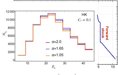
Figure 1: The density profile snapshot at time $t=5$ s post collapse [77]. The various regions of interest in the shock wave profile are labelled.

The turbulence is included in our model by adding a random field $F(r)$ as

$$V(r)=\big{(}1+F(r)\big{)}V_{0}(r)$$ (2)

The random field $F(r)$ is defined in the following way

$$F(r)=\begin{cases}C_{*}\tanh{\bigg{(}\frac{r-r_{\rm rs}}{\lambda}\bigg{)}}\tanh{\bigg{(}\frac{r_{\rm fs}-r}{\lambda}\bigg{)}}\times F_{\rm rand}(r),\hskip 5.69046ptr_{\rm rs}\leq r\leq r_{\rm fs}\,,\\ 0,\hskip 5.69046pt\text{elsewhere}\,,\end{cases}$$ (3)

where $C_{*}$ is the amplitude of the fluctuations, $F_{\rm rand}(r)$ is a real-valued homogenous Gaussian scalar random field. The reverse shock position is given by $r_{\rm rs}$ while the forward shock position is $r_{\rm fs}$. The $\tanh$ terms suppress the fluctuations close to the shocks and prevent discontinuities at $r_{\rm rs}$ and $r_{\rm fs}$. The parameter $\lambda$ is the length scale over which the fluctuations reach their extent. We choose $\lambda=100$ km.

The standard way of calculating the evolution of the neutrino wavefunctions involves numerically solving the Schr$\ddot{\rm o}$dinger equation directly. Unfortunately for irregular potentials (matter densities), this method is not efficient. In particular, the current scenario has turbulences making the matter potential highly noisy and the standard scenario for solving such problems is unsuitable. Hence, we use the slab approximation [98] to calculate the spatial evolution of the neutrino wavefunctions.

In this approximation, the density profile is approximated by a series of slabs of constant density. We discretize the spatial dimension of physical size $L$ into $n$ slabs, thus the width of each slab is, $\Delta x=L/n$. In such a discretization scheme, the starting point is given by $x_{0}$ and the boundaries of the slabs are at $x_{1},x_{2},\dots,x_{n}$. The mass eigenstates of the neutrinos propagate as plane waves in constant density regions with phases given by ${\rm exp}{(\pm i\Delta m_{M}^{2}\Delta x/4E)}$, where the effective mass-squared difference in matter is given by

$$\Delta m^{2}_{M}=\sqrt{\Big{(}\hbox{$\Delta m^{2}$ }\cos{(2\theta)}-A_{CC}\Big{)}^{2}+\Big{(}\hbox{$\Delta m^{2}$ }\sin{(2\theta)}\Big{)}^{2}}\,,$$ (4)

with $\theta$ being the vacuum mixing angle. $A_{CC}$ is the effective effective charge current potential,

$$A_{CC}(x)=2\sqrt{2}EG_{F}n_{e}(x)\,,$$ (5)

All the information about the matter density profile is provided by this term.

The wavefunction in the flavor basis is given by,

$$\bm{\Psi}_{e}=\langle x|\nu_{e}\rangle=\begin{pmatrix}\psi_{ee}\\ \psi_{ex}\end{pmatrix}$$ (6)

The wavefunction at the boundaries is joined according to the following scheme

$$\bm{\Psi}_{e}(x_{n})=\left[U_{M}\ \mathcal{U}_{M}(x_{n}-x_{n-1})\ U_{M}^{\dagger}\right]_{(n)}\left[U_{M}\ \mathcal{U}_{M}(x_{n-1}-x_{n-2})\ U_{M}^{\dagger}\right]_{(n-1)}\dots\left[U_{M}\ \mathcal{U}_{M}(x_{1}-x_{0})\ U_{M}^{\dagger}\right]_{(1)}\bm{\Psi}_{e}(x_{0})\,,$$ (7)

where,

• the unitary evolution operator in each slab diagonal basis $\mathcal{U}_{M}(\Delta x)$ is given by,

  $$\mathcal{U}_{M}(\Delta x)=\rm diag\Bigg{(}exp{(+i\Delta m_{M}^{2}\Delta x/4E)},exp{(-i\Delta m_{M}^{2}\Delta x/4E)}\Bigg{)}\,,$$ (8)

• $U_{M}$ is the unitary mixing matrix in matter given by

  $$U_{M}=\begin{pmatrix}\cos{\theta_{M}}&\sin{\theta_{M}}\\ -\sin{\theta_{M}}&\cos{\theta_{M}}\end{pmatrix}\,,$$ (9)

  where the effective mixing angle in matter $\theta_{M}$ is

  $$\tan{(2\theta_{M})}=\frac{\tan{(2\theta)}}{1-\frac{A_{CC}}{\Delta m^{2}\cos{(2\theta)}}}\,.$$ (10)

• The notation $\left[\dots\right]_{(i)}$ indicates that all the matter-dependent quantities inside the brackets need to be evaluated with the matter density profile of the $i$-th slab, where the slab goes from $x_{i-1}$ to $x_{i}$.

The wavefunction in the matter basis can be easily obtained using (7) and (9) as

$$\bm{\Phi}=\begin{pmatrix}\phi_{1}\\ \phi_{2}\end{pmatrix}=U_{M}^{-1}\bm{\Psi}_{e}\,.$$ (11)

The probability that a neutrino of flavor $\alpha$ is found in some flavor $\beta$ after passing through the matter profile is given by

$$P_{\nu_{\alpha}\rightarrow\nu_{\beta}}=|\psi_{\alpha\beta}|^{2}\,.$$ (12)

Similarly, the corresponding survival probability of the matter eigenstate is given by $P_{\nu_{i}\rightarrow\nu_{j}}=|\bm{\Phi}_{i}|^{2}$. The adiabaticity parameter, which is an important quantity to understand the changes in oscillation and transition probabilities related to neutrino propagation, is defined as [98]

$$\gamma=\frac{\Delta m^{2}_{M}}{4E_{\nu}|d\theta_{M}/dx|}=\frac{(\Delta m_{M}^{2})^{2}}{2E_{\nu}\ ({\rm sin}\ 2\theta_{M})\ |dA_{{\rm CC}}/dx|}\,.$$ (13)

Armed with this, we can investigate the propagation of neutrinos in an irregular potential.

III Turbulence: Numerical ansatz

In this section, we discuss the Randomization Method used to implement stochastic fluctuations following a power-law on top of a smooth matter profile.

III.1 The Randomization Method: Generating the turbulence

In previous works, the authors of [84] used the Randomization Method [99] to generate and sample the turbulence. In [86], a slightly advanced version of the randomization method - ‘Variant C’ was used. For this work, we will use the Variant C of the randomization method to generate the turbulence. It is important to note here that in this method the modes are distributed in a logarithmic scale which makes the distribution scale-invariant by ensuring that the realizations are uniform over the decades of length scales considered in the work. We summarize the method below.

Let the wavenumber space from which we draw the wavenumbers have a size $\Delta$, such that, $\Delta=[0,\infty)$. For numerical implementation, the space $\Delta$ is divided into $n$ non-intersecting intervals $\Delta_{j}$, such that, $\Delta=\cup_{j=1}^{n}\Delta_{j}$. We then select $n_{0}$ independent random wavenumbers from each of these intervals $\Delta_{j}$, which can now be indexed as $k_{jl}$, where, $l=1,2,\dots,n_{0}$. The selection of the $k_{jl}$’s are according to the probability distribution function $p_{j}(k)$ defined as

$$p_{j}(k)=\begin{cases}2E(k)/\sigma_{j}^{2},\hskip 14.22636pt\text{for }k\in\Delta_{j}\,,\\ 0,\hskip 14.22636pt\text{for }k\notin\Delta_{j}\,,\end{cases}$$ (14)

where $E(k)$ is the power spectrum, which we assume to be of the following form,

$$E(k)=(\alpha-1)\bigg{(}\frac{k_{*}}{k}\bigg{)}^{\alpha}\,.$$ (15)

In the above definition of the power spectrum, $\alpha$ is the spectral index, $k_{*}=2\pi/\lambda_{*}$ is the wavenumber cutoff, i.e., the cutoff that decides the longest non-zero turbulence wavelength ($\lambda_{*}$) and hence the smallest wavenumber. Thus, it can be referred to as the driving scale for our turbulence model [87]. For this work, we treat the spectral index $\alpha$ as a free parameter that is varied and the corresponding sensitivity of the next-generation neutrino detectors is tested. We choose, $\lambda_{*}=2(r_{\rm fs}-r_{\rm rs})$, which is twice the distance between the positions of the reverse and forward shocks. In Eq. (14), $\sigma_{j}^{2}=2\int_{\Delta_{j}}E(k)dk$.

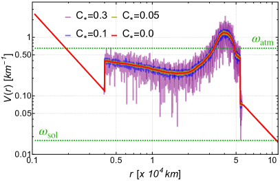
Figure 2: The effective matter potential profile for fixed $\alpha=-5/3$ and different values of the normalization $C_{*}$. The case where turbulence is absent is represented by $C_{*}=0$ (solid red curve). The value of $\omega=\Delta m^{2}/(2E_{\nu})$ is also shown as a dashed green line corresponding $\Delta m^{2}_{\rm atm}=2.6\times 10^{-3}\ \rm eV^{2}$, $\Delta m^{2}_{\rm sol}=6.9\times 10^{-5}\ \rm eV^{2}$ for $E_{\nu}=10\ \rm MeV$.

We can now define $F_{\rm rand}(r)$ (see Eqs. (2) and (3)) as

$$F_{\rm rand}(r)=\sum_{j=1}^{n}\frac{\sigma_{j}}{\sqrt{n_{0}}}\sum_{l=1}^{n_{0}}\left[\xi_{jl}\ \text{cos}\big{(}2\pi k_{jl}r\big{)}+\eta_{jl}\ \text{sin}\big{(}2\pi k_{jl}r\big{)}\right]\,,$$ (16)

where, $\xi_{jl}$ and $\eta_{jl}$ are standard Gaussian random variables, which are independent of each other and of $k_{jl}$, have zero mean, and unit variance. Note that the indices $j=1,2,\dots,n$ and $l=1,2,\dots,n_{0}$. In this strategy of stratified sampling of the wavenumber bins, we choose the sampling bins such that they are equally spaced in the log-space, that is with respect to $\text{ln }k$. Thus we have, for a given index $j$, $\hat{k}_{j+1}=q\hat{k}_{j}$, where $q$ is some ratio parameter of the geometric distribution which defines the wavenumber intervals $\Delta_{j}=(\hat{k}_{j},\hat{k}_{j+1}]$. Since we have a minimum wavelength in our model, we have $\hat{k}_{1}=k_{*}$. The bounded domain for $k$ also introduces the constraint, $k\leq k_{\max}$, where we choose $k_{\max}=100$, such that $\hat{k}_{n+1}=k_{\max}$. For this work, we chose $n=4$ and $n_{0}=40$. We have also verified that pushing $n$ and $n_{0}$ to higher values of $5$ and $50$ respectively does not change the results. It is important to note here that this strategy of stratified sampling is efficient in way that allows us to work with a comparatively low value of total number of modes, $\mathcal{O}(100)$, to give us accurate and physical scale independent results, as compared to just sampling the modes trivially, thus, gaining some computational advantage. The density profile extends from $r_{\rm start}=0.105\times 10^{4}$ km to $r_{\rm end}=11.35\times 10^{4}$ km. This region is sampled in spatial steps of $\delta x=10$ km. The turbulence is introduced to this density profile, starting at the reverse shock position which is at, $r_{\rm rs}=0.39\times 10^{4}$ km and it is terminated at the position of the forward shock, $r_{\rm fs}=5.6\times 10^{4}$ km. The region of turbulence has the same spatial discretization scale as the original density profile ($=10$ km).

As stated earlier, the primary parameters that we vary and examine in this work are the amplitude associated with the turbulence $C_{*}$ and the power spectral index $\alpha$. In Fig. 2, we show the effective matter potential for a fixed $\alpha=-5/3$ and various values of $C_{*}$. The red thick line is the case when turbulence is absent, that is, $C_{*}=0$. This is essentially the same curve as shown in Fig. 1 (solid blue curve) rescaled to convert the matter density to effective potential using natural units $\hbar$ and $c$. As the amplitude of turbulence increases, the fluctuations grow as expected. The effects of this variation in the amplitude on the survival probabilities for neutrinos are discussed in the following section. It is important to note here that we want to focus on the effects associated solely with the non-adiabaticity at the forward and reverse shocks, hence we artificially smoothed the contact discontinuity so as to avoid any non-adiabaticity effects arising from it.

III.2 Results

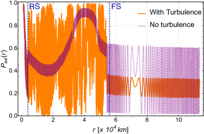
(a) (a)

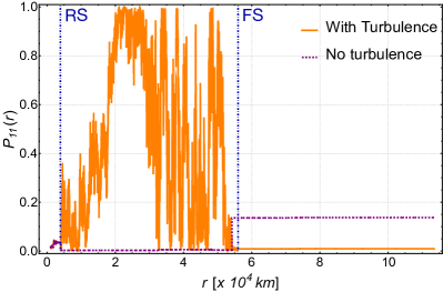
(b) (b)

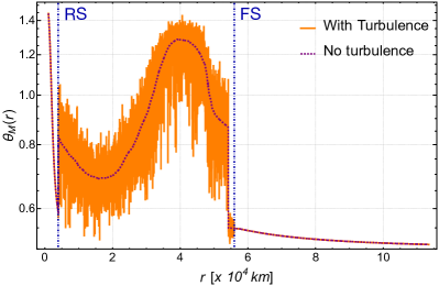
(c) (c)

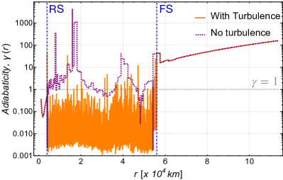
(d) (d)

Figure 3: Comparison between the scenarios when turbulence is present ($C_{*}=0.3,\alpha=-5/3$) (solid orange curves) and when turbulence is absent ($C_{*}=0$) (dashed purple curves). (a) The $\nu_{e}$ survival probability, $P_{ee}(r)$. (b) The survival probability for the first instantaneous matter eigenstate, $P_{11}(r)$. (c) The effective mixing angle in matter, $\theta_{M}(r)$ from Eq. (10); (d) The adiabaticity parameter, $\gamma(r)$, from Eq. (13). The reverse shock (RS) and forward shock (FS) are shown as dot-dashed dark blue lines. We assume $\theta_{0}=0.09967$ rads, $\Delta m_{vac}^{2}=2.6\times 10^{-3}\rm eV^{2}$, and $E_{\nu}=10$ MeV.

In this section, we discuss the results obtained by solving for neutrino flavor propagation through the matter profile as shown in Fig. 2. The two primary scenarios we are interested in are when turbulence is absent and when turbulence has a high amplitude. Thus, we compare the results for $C_{*}=0$ (which we label as without turbulence) and $C_{*}=0.3$ (which we label as with turbulence) respectively to implement the above scenarios. The choice of $C_{*}=0.3$ is representative of an extreme case where complete flavor depolarization occurs and the oscillation signatures are washed out.

The results are shown in Fig. 3 for the electron neutrino survival probability ($P_{ee}(r)$), the survival probability for the first instantaneous matter eigenstate ($P_{11}(r)$), the effective mixing angle in matter ($\theta_{M}$) and the adiabaticity parameter ($\gamma(r)$) as $\nu_{e}$ propagates through the effective matter profile from $r_{\rm start}$ to $r_{\rm end}$. In Fig. 3a we show the survival probability ($P_{ee}(r)$) for $\nu_{e}$ as a function of distance for the cases of with (solid orange) and without (dotted purple) turbulence. We note that the survival probability initially starts from unity, corresponding to a pure $\nu_{e}$ state. The position of reverse shock introduces a drop in the survival probability. Between the forward and the reverse shocks, the behaviour of $P_{ee}(r)$ is clearly distinct for the cases with and without turbulence. The propagation of the neutrinos in the presence of turbulence is extremely non-adiabatic due to the highly fluctuating background matter density. A better understanding can be achieved by studying $P_{11}(r)$ (in Fig. 3b), which is expected to track the changes in the density. The matter eigenstate survival probability shows a jump due to non-adiabatic evolution corresponding to the density jumps. While the case without turbulence has jumps only at the positions of the reverse and forward shocks, the case with turbulence has numerous jumps.

A similar trend can be seen in the effective mixing angle in the matter for the two cases, as shown in Fig. 3c. The case without turbulence exhibits a maximal change in $\theta_{M}$ at the locations of the forward and reverse shocks, whereas, in the presence of turbulence, $\theta_{M}$ has large jumps throughout the density profile. To demonstrate the non-adiabaticity associated with the neutrino flavor evolution, Fig. 3d shows the associated adiabaticity parameter, $\gamma(r)$. A highly non-adiabatic evolution is characterized by $\gamma(r)<<1$. We see that for the case with turbulence between the reverse and the forward shocks, the adiabaticity parameter is much smaller than 1, implying a highly non-adiabatic evolution. The turbulence is only seeded between the forward and reverse shocks, so beyond the forward shock, the evolution once again becomes adiabatic in the absence of any further shocks or turbulence. This can be seen from Figs. 3b and 3d, where in the former case, the transition probability does not show any jumps beyond the forward shock, whereas in the latter case, $\gamma(r)>>1$ in the same region, implying adiabatic evolution.

III.3 On the double-dip associated with shocks

The presence of shocks characterized by rapid changes in the density profile can have imprints on the neutrino oscillation probabilities. The MSW resonance associated with neutrino oscillations is given by, $\Delta m^{2}{\rm cos}2\theta/(2E_{\nu})=\pm\sqrt{2}G_{F}Y_{e}\rho$, where $G_{F}$ is the Fermi constant, $Y_{e}$ is the electron fraction, and $\rho$ is the matter density. Depending on the mass-squared difference corresponding to solar or atmospheric neutrinos, the resonances are classified as L-resonance (low density) and H-resonance (high density) respectively. The propagation of the shockwave through the densities corresponding to H-resonance regions can break adiabaticity leading to distinctive features in the neutrino energy spectra.

As discussed in Sec. I, numerical simulations hint towards the presence of both forward and reverse shocks in the matter density profile, resulting in a double-dip feature in the neutrino spectra [77].

Figure 4: The average survival probability ($\langle P_{ee}\rangle$) with neutrino energy ($E_{\nu}$) for different amplitudes of turbulence associated with the density profile (see Fig. 2).

In Fig. 4 we show the average survival probability for $\nu_{e}$ as a function of the neutrino energy ($E_{\nu}$). Note the presence of the double-dip feature (solid red curve) in the neutrino spectra corresponding to the density profile (in Fig. 2) in the absence of turbulence $(C_{*}=0)$. The first peak corresponds to $E_{\nu}\sim 18$ MeV and is due to the forward shock. Following the first peak, the adiabatic transitions corresponding to the forward and reverse shocks partially cancel out to give the valley. Finally, a second peak appears for $E_{\nu}\gtrsim 60$ MeV which is due to the neutrinos crossing one of the forward or reverse shocks.

We now aim to study the effects of the presence of turbulence on the double-dip feature in the neutrino spectra. The results are shown in Fig. 4 for a range of turbulence amplitudes given a fixed value of $\alpha=-5/3$. Interestingly, we find that the double-dip feature vanishes as the amplitude of turbulence increases leading to highly non-adiabatic flavor evolution. For $C_{*}>0.01$, the first peak disappears. As the value of $C_{*}$ is increased, a gradual wash-out of the feature is seen. In fact, for the maximum value of $C_{*}$ used in this work, i.e., $C_{*}=0.3$, the survival probability averages to $1/2$, signifying complete flavor depolarization. Thus, the presence of turbulence can completely wash away the double-dip feature in the neutrino energy spectra associated with forward and reverse shocks. This can be used to probe the presence of hydrodynamic turbulence in core-collapse supernovae.

III.4 Revisiting previous analytical results for a simplified model of turbulence

In [83], the effects of a simple model for turbulence on neutrino propagation in supernovae were studied. In particular, analytical estimates corresponding to neutrino flavor depolarization in the presence of a Kolmogorov-type turbulence were derived. The authors argued that evidence from numerical simulations hints towards the development of Kolmogorov cascades due to various instabilities. In such a turbulence scenario, the Fourier transform of the velocity correlator has the following form,

$$C(k)\equiv\int dx\langle\delta n(0)\delta n(x)\rangle e^{-ikx}=C_{0}k^{\alpha}\,,$$ (17)

where $\alpha=-5/3$. The matter potential, $A(x)$, was assumed to be linear and turbulent random noise was introduced as

$$A(x)=x+F\sum_{k=1}^{600}k^{\beta}\cos{\Big{(}kx+\phi(k)\Big{)}}\,,$$ (18)

where $F$ is the amplitude or normalization factor for the noise, $k$ is the mode number, $\beta=\alpha/2$, and $\phi(k)$ is a random phase which is a random value between $0$ and $2\pi$ for every mode $k$. The above equation can be compared to Eq. (2) used in this work.

We reproduce the numerical results from [83] using the same parameters to check our numerical code. We show the result in Fig. 5a. The spatial coordinate goes from $x=-100$ to $x=100$, $\Delta=50$, and $\theta=0.1$. We choose $\Delta x=0.1$. The agreement between our results and the same obtained by the previous work is good. We find that for low turbulence amplitudes, the effect on survival probability is less pronounced, which is expected and matches with our own analysis discussed above. When the turbulence amplitude is increased from $F\sim 0.2$ to higher values, a power law develops. The power law rise seen in the figure can be explained using an analytical estimate derived in [83],

$$P^{\rm rise}\approx 0.84\ \frac{G_{F}C_{0}(2\Delta{\rm sin}\ 2\theta_{13})^{-2/3}}{\sqrt{2}|n_{0}^{\prime}|}\,,$$ (19)

where $n_{0}^{\prime}$ is related to the spatial derivative of the matter density. We note that for values of $F\gtrsim 0.05$, a complete flavor depolarization happens, implying the flavor constitution becomes equal for $\nu_{e}$ and $\nu_{x}$, in the two-flavor oscillation scenario considered here.

We extend the analysis in [83] by studying the variation of the average electron neutrino survival probability ($\langle P_{ee}\rangle$) in the $\beta-F$ plane. The result, in the form of a density plot for the average probability, is shown in Fig. 5b. A rainbow color scheme is used to illustrate $\langle P_{\rm ee}\rangle$, where the violet end of the spectrum implies $\langle P_{\rm ee}\rangle\sim 0$ and the red end signifies $\langle P_{\rm ee}\rangle\sim 1$. The area where complete flavor depolarization occurs is shown by a greenish-yellow shade corresponding to $\langle P_{\rm ee}\rangle\sim 0.5$. For $\beta\sim 0$, we find that $\langle P_{\rm ee}\rangle\sim 0.5$ for any given value of the turbulence amplitude $F$. As $\beta$ decreases to $-1$, higher amplitudes of turbulence lead to flavor depolarization. This generalizes the results of  [83] and confirms that for large values of $F$, flavor depolarization holds for other values of $\beta$ as well.

There are distinct differences between the analysis in [83] and our current work. We assume a more realistic matter density profile based on actual simulations in contrast to the linear profile assumed for simplicity in the former work. While the simple profile helps in getting some analytical estimates, the effects of a realistic profile need to be addressed numerically and lead to more realistic predictions for the upcoming detectors. Furthermore, the seeding of the turbulence in this work uses a variant of the Randomization method which is different from the simple random noise turbulence used in the previous work.

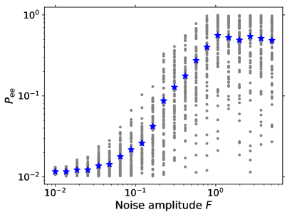
(a) (a)

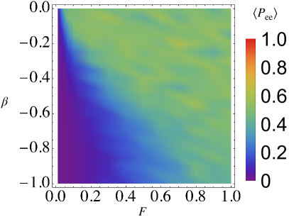
(b) (b)

Figure 5: (a) The electron neutrino survival probability as a function of the noise amplitude $F$ for $\beta=-5/6$, to match with the results of [83] (see Fig. 1 there); (b) The electron neutrino survival probability as a function of $\beta$ ranging from $-1$ to $0$ for various values of $F$. Each data point in the numerics was repeated for $66$ times and the average value was used.

IV Events rates and statistical analysis

In previous sections, we discussed the effects of turbulence on the neutrino signatures and survival probabilities. This section focuses on the prospects and the capabilities of the upcoming neutrino detectors to constrain the parameters associated with turbulence, in particular, the amplitude $(C_{*})$ and the spectral index $(\alpha)$. The detectors we consider for this work are the Deep Underground Neutrino Experiment (DUNE) and Hyper-Kamiokande (HK). While the former is largely sensitive to a flux of $\nu_{e}$, the latter is better suited for detecting the $\bar{\nu}_{e}$ flux.

The supernova neutrino spectrum at the source (the neutrinosphere) is assumed to be a pinched Fermi-Dirac spectrum [100],

$$\frac{dN_{\nu}^{\rm src}(E_{\nu})}{dE_{\nu}}=\frac{L_{\nu}}{\langle E_{\nu}\rangle^{2}}\frac{(1+\alpha_{\nu})^{(1+\alpha_{\nu})}}{\Gamma(1+\alpha_{\nu})}\bigg{(}\frac{E_{\nu}}{\langle E_{\nu}\rangle}\bigg{)}^{\alpha_{\nu}}{\rm exp}\bigg{(}-(1+\alpha_{\nu})\frac{E_{\nu}}{\langle E_{\nu}\rangle}\bigg{)}\,,$$ (20)

where $N_{\nu}^{\rm src}$ is the number of neutrinos at the source for any given flavor with energy $E_{\nu}$, $L_{\nu}$ is the neutrino luminosity for that particular flavor, $\langle E_{\nu}\rangle$ is the mean neutrino energy, $\alpha_{\nu}$ is a pinching parameter associated with the given flavor. Considering the cooling phase, we choose $L_{\nu_{e}}=L_{\bar{\nu}_{e}}=5\times 10^{51}$ erg, $L_{\nu_{x}}=L_{\bar{\nu}_{x}}=10^{52}$ erg, $\langle E_{\nu_{e}}\rangle=12$ MeV, $\langle E_{\bar{\nu}_{e}}\rangle=15$ MeV, $\langle E_{\nu_{x}}\rangle=\langle E_{\bar{\nu}_{x}}\rangle=18$ MeV, and $\alpha_{\nu_{e}}=\alpha_{\bar{\nu}_{e}}=\alpha_{\nu_{x}}=\alpha_{\bar{\nu}_{x}}=3$. The neutrinos emitted from the neutrinosphere then propagate through the matter profile encountering the forward and reverse shocks, along with the turbulence which leads to neutrino oscillations. Let $P_{ee}$ be the survival probability of $\nu_{e}$ while propagation. In this case, the number of $\nu_{e}$ neutrinos at the end of the matter profile is given by

$$\frac{dN_{\nu_{e}}^{\rm SN}(E_{\nu})}{dE_{\nu}}=P_{ee}(E_{\nu})\frac{dN_{\nu_{e}}^{\rm src}(E_{\nu})}{dE_{\nu}}+\big{(}1-P_{ee}(E_{\nu})\big{)}\frac{dN_{\nu_{x}}^{\rm src}(E_{\nu})}{dE_{\nu}}\,,$$ (21)

where $N_{\nu_{e}}^{\rm SN}$ is the number of $\nu_{e}$ after the initial neutrino spectra from the neutrinosphere have propagated through the matter profile. Similarly one can obtain the spectra for $\bar{\nu}_{e}$. Once the neutrinos leave the supernova they propagate through the interstellar medium to reach Earth. This can be effectively treated as propagation in vacuum. The vacuum survival probability for $\nu_{e}$ is given by

$$P_{ee}^{\rm vac}(E_{\nu})=1-{\rm sin}^{2}2\theta\ {\rm sin}^{2}\bigg{(}\frac{\Delta m^{2}R}{4E_{\nu}}\bigg{)}\simeq 1-\frac{1}{2}{\rm sin}^{2}2\theta=0.58\,,$$ (22)

where $\theta_{\rm vac}$ is the vacuum mixing angle and $\Delta m^{2}_{\rm vac}$ is the vacuum mass-squared difference. We assume $\theta_{\rm vac}=0.9967$ rads and $\Delta m^{2}_{\rm vac}=2.6\times 10^{-3}\rm eV^{2}$. Thus the neutrino spectra at the Earth, neglecting Earth-matter effects, is given by

$$\frac{dN_{\nu_{e}}^{\rm earth}(E_{\nu})}{dE_{\nu}}=P_{ee}^{\rm vac}(E_{\nu})\frac{dN_{\nu_{e}}^{\rm SN}(E_{\nu})}{dE_{\nu}}+\big{(}1-P_{ee}^{\rm vac}(E_{\nu})\big{)}\frac{dN_{\nu_{x}}^{\rm SN}(E_{\nu})}{dE_{\nu}}\,.$$ (23)

A similar analysis can be repeated for obtaining the $\bar{\nu}_{e}$ spectra on earth which will be relevant for HK. We do not consider earth matter effects for this work.

The total number of neutrinos of a given species $\alpha$ ($N_{\nu_{\alpha}}$) detected in a neutrino detector from a source at a distance $R$ is given by

$$N_{\nu_{\alpha}}=\Delta t\frac{N_{\rm tar}}{4\pi R^{2}}\int dE_{r}\int dE_{t}\ \frac{dN_{\nu_{\alpha}}^{\rm earth}(E_{t})}{dE_{t}}\sigma_{\nu_{\alpha}}(E_{t})W(E_{r},E_{t})\,,$$ (24)

where $N_{\rm tar}$ is the number of targets for a given channel in the detector fiducial volume, $\sigma_{\nu_{\alpha}}$ is the neutrino interaction cross-section with the targets for the relevant channel, $\Delta t$ is the duration for which we assume the density profile to remain approximately fixed and similar to what is considered for the matter profile, and $W$ is the Gaussian energy resolution function which depends on the intrinsic properties of the detector. The experimentally reconstructed energy in the detector is given by $E_{r}$ and the actual neutrino energy is given by $E_{t}\equiv E_{\nu}$. We fix the distance to the supernova at $R=10$ kpc for our current work. The energy resolution function is defined as [101]

$$W(E_{r},E_{t})=\frac{1}{\sqrt{2\pi}\sigma_{E}(E_{r})}\exp{\bigg{(}-\frac{1}{2}\frac{(E_{r}-E_{t})^{2}}{\sigma_{E}(E_{r})^{2}}\bigg{)}}\,.$$ (25)

The sensitivity of the neutrino detectors for different values of $C_{*}$ and $\alpha$ is estimated using a simple $\chi^{2}$ estimator

$$\chi^{2}=\frac{\big{(}N_{\rm obs}-N_{\rm exp}\big{)}^{2}}{N_{\rm obs}}\,,$$ (26)

where $N_{\rm obs}$ is the number of neutrino events observed in the neutrino detector, $N_{\rm exp}$ is the expected number of neutrino events in the detector. We fix $N_{\rm exp}$ to the case when $C_{*}=0.1$, and $\alpha=1.65$, corresponding to the Kolmogorov turbulence, unless otherwise specified. We consider $\Delta t=1\,{\rm s}$.

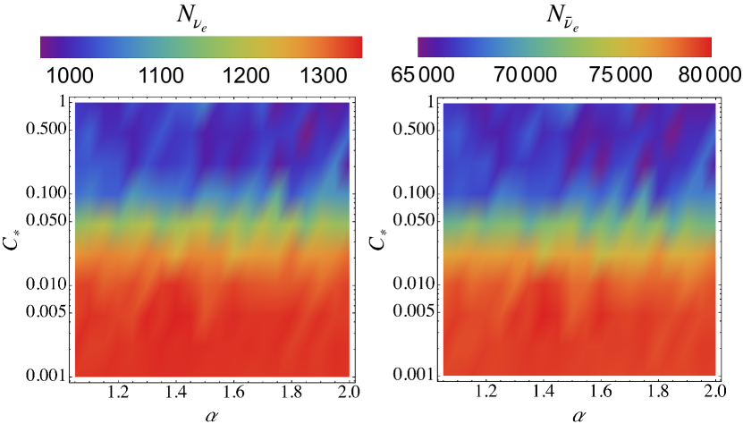
Figure 6: Density plot to show the total number of $\nu_{e}$ events for DUNE (left) and $\bar{\nu}_{e}$ events for HK (right) on the $C_{*}-\alpha$ plane. The source is assumed to be at a distance of $R=10$ kpc. See text for details on the other parameters used.

IV.1 DUNE

The DUNE experiment [102] consists of a near and a far detector separated by $1300$ km. The former is located at Fermilab, Illinois while the latter is located about $1.5$ km below the ground at the Stanford Underground Research Facility (SURF), South Dakota. The far detector is a liquid argon time projection chamber (LArTPC) with $70$ kt (fiducial mass of $40$ kt) of liquid argon. We will focus on the far detector in this work.

The relevant interaction channel for supernova neutrinos is the charged current interaction of electron neutrinos with argon nuclei, $\nu_{e}+^{40}{\rm Ar}\rightarrow^{40}{\rm K}^{*}+e^{-}$. We use $N_{\rm tar}=6\times 10^{32}$. The interaction cross-section $\sigma_{\nu_{e}}$ associated with the $\nu_{e}-\rm Ar$ interaction cross section is taken from [103]. The energy resolution for DUNE is taken to be $\sigma_{E}/{\rm MeV}=0.11\sqrt{E_{r}/{\rm MeV}}+0.02E_{r}/{\rm MeV}$.

The result for the total number of electron neutrino events $N_{\nu_{e}}$ for DUNE is shown in the left panel of Fig. 6 as a density plot in the $C_{*}-\alpha$ plane. The color map uses a rainbow template to denote the lowest number of events in violet and the highest in red. For a typical galactic scale supernova ($R\sim 10$ kpc) we have $\sim 10^{3}$ events in DUNE in the $\nu_{e}$ channel. There are two interesting aspects that we note right away - (a) as $\alpha$ varies from $1.0$ to $2.0$, the number of events $N_{\nu}$ does not change significantly, which implies that it would be difficult to put constraints on the value of $\alpha$ using the DUNE detector; (b) as $C_{*}$ is varied from $0.001$ to $1.0$ the number of events in the DUNE detector has a significant variation and goes from $\sim 1350$ (red) for lower values of $C_{*}\sim 0.001$ to $\sim 900$ (violet) for large values of $C_{*}\sim 1.0$. Thus, DUNE can be used to place constraints on the value of $C_{*}$ for a typical galactic supernova in the near future. We discuss the two points below using a $\chi^{2}$ plot as discussed below.

The significant variation of the number of events with $C_{*}$ is confirmed in Fig. 7a, which shows the variation of $\chi^{2}$ versus $C_{*}$ for $\alpha=1.65$. The null hypothesis is considered to be $C_{*}=0.1$. We note that for low values of $C_{*}<0.05$, the $\chi^{2}$ starts growing and it increases as the amplitude of turbulence decreases. However, for larger values of $C_{*}>0.05$, constraints become weak. To get a better understanding of this behaviour, we compare the event spectra for different values of $C_{*}$ in Fig. 7c. The null hypothesis $(C_{*}=0.1)$ is shown with a dotted dark blue line. The cases corresponding to $C_{*}=0.005,0.02$, and $0.5$ are shown as solid purple, orange, and red lines. On comparing the case of $C_{*}=0.005$ with the expected case we see a significant difference in the number of events in the energy bins above $17$ MeV leading to the high value of $\chi^{2}$. As $C_{*}$ increases the number of events in the energy bins becomes similar to the expected case of $C_{*}=0.1$ explaining the trend of $\chi^{2}$ as seen in Fig. 7a.

The variation over $\alpha$ does not have a specific trend for any value of $C_{*}$ and the $\chi^{2}$ values obtained are extremely low and we do not show them here. This is evident from Fig. 8a where we show the event spectra for $\alpha=1.05$ (solid orange), $1.65$ (dashed dark blue), and $2.0$ (solid purple) for $C_{*}=0.1$. The expected scenario for this case is again chosen to be $C_{*}=0.1$ and $\alpha=1.65$ shown as the dashed dark blue line. We note that the spectra for all the three cases shown look very similar to the expected case in dotted dark blue, explaining the low values of $\chi^{2}$. This highlights the ineffectiveness of DUNE to put constraints on the value of $\alpha$.

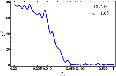
(a) (a)

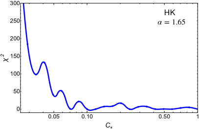
(b) (b)

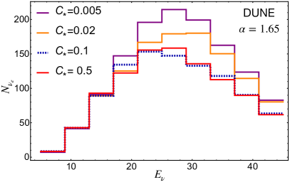
(c) (c)

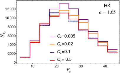
(d) (d)

Figure 7: (a) Plot of $\chi^{2}$ estimator for different values of $C_{*}$ for DUNE assuming $\alpha=1.65$ (corresponding to Kolmogorov turbulence); (b) same as (a) but for HK; (c) The expected number of $\nu_{e}$ events per energy bin for DUNE assuming $\alpha=1.65$ and $C_{*}=0.005$ (solid purple), $0.02$ (solid orange), and $0.5$ (solid red). The $N_{\rm exp}$ for the $\chi^{2}$ estimator is considered to be the case when $C_{*}=0.1$ and $\alpha=1.65$, which is shown as a dotted dark blue line; (d) same as (c) but for HK where $\bar{\nu}_{e}$ events are considered.

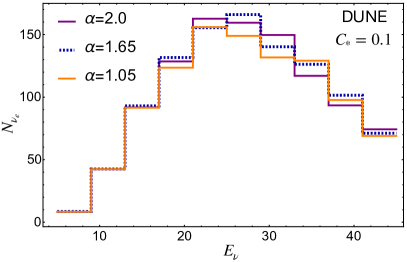
(a) (a)

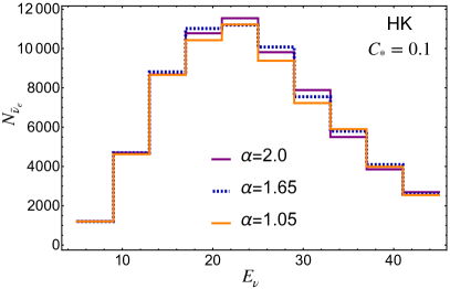
(b) (b)

Figure 8: The expected number of $\nu_{e}$ and $\bar{\nu}_{e}$ events per energy bin corresponding to DUNE (left) and HK (right) for a fixed value of $C_{*}=0.1$ and different values of $\alpha=1.05$ (solid orange), $1.65$ (dotted dark blue), and $2.0$ (solid purple) respectively. The source is assumed to be at a distance of $R=10$ kpc.

IV.2 Hyper-Kamiokande

Hyper-Kamiokande (HK) [104] is an upcoming $260$ kton (fiducial $187$ kton) liquid scintillator detector, being built at the Kamioka Observatory in Japan. It is an upgrade to the Super-Kamiokande detector but with around $10$ times the fiducial volume. It will consist of two tanks of ultrapure water acting as the medium for neutrino detection. The primary detection channel in HK is the inverse-beta decay (IBD), $\bar{\nu}_{e}+p\rightarrow e^{+}+n$. We use the IBD cross-section from [105]. Similar to Super-Kamiokande, the energy resolution for HK is given by $\sigma_{E}/{\rm MeV}=0.6\sqrt{E_{r}/{\rm MeV}}$ [103]. The number of targets for HK is assumed to be $1.2\times 10^{35}$.

The density plot for the number of $\bar{\nu}_{e}$ events for HK in the $C_{*}-\alpha$ plane is shown in the right panel of Fig. 6. The details of the colors used are discussed in Sec. IV.1. We have $\sim 7\times 10^{4}$ $\bar{\nu}_{e}$ events for a typical galactic scale supernova ($R=10$ kpc). This number is much higher than DUNE owing to the larger number of targets. This already hints at the possibility that HK would be a better detector than DUNE at constraining the parameter range for turbulence. However, similar to DUNE, the variation in $N_{\bar{\nu}_{e}}$ is insignificant across the different values of $\alpha$ for a given value of $C_{*}$.

Using HK, relatively strong constraints can be placed on the amplitude of turbulence as seen by the variation in $N_{\bar{\nu}_{e}}$ with $C_{*}$ for a fixed value of $\alpha$ in the right panel of Fig. 6. This is also evident from Fig. 7b where we have very large values of $\chi^{2}$ for $C_{*}\lesssim 0.05$, keeping $\alpha$ fixed at $1.65$. To confirm our results, we show the event spectra for $\alpha=1.65$ and different values of $C_{*}$ in Fig. 7d. Once again, the expected case is assumed to be $C_{*}=0.1$ and $\alpha=1.65$ and is shown in dotted dark blue. We note that similar to the case of DUNE, for $E_{\nu}\leq 20$ MeV, the spectra are similar among all the cases, however for $E_{\nu}>20$ MeV, there is a significant difference in the spectra between $C_{*}=0.1$ and $C_{*}=0.005$ (solid purple line) and $C_{*}=0.02$ (solid orange line) leading to the comparatively high values of $\chi^{2}$. However, for $C_{*}=0.5$ (solid red line) the event spectra look similar to the expected case giving a low value of $\chi^{2}$ as seen in Fig. 7b.

Finally in Fig. 8b, we show the event spectra for $C_{*}=0.1$ for different values of $\alpha$. The spectra look similar to the expected case of $C_{*}=0.1$, indicating that HK, while sensitive, would not be able to put very strong constraints on $\alpha$.

V Conclusions and Implications

Neutrino propagation through a turbulent medium leads to high degrees of non-adiabaticity. Hydrodynamical simulations of core-collapse supernova hint towards the presence of various instabilities in the region behind the shock, leading to the matter profile becoming turbulent. Such a turbulent medium can leave its signature on the neutrino spectra, thereby allowing future neutrino detectors to probe the strength of turbulence inside a core-collapse supernova. In this work, we performed a detailed study of the effects of turbulence on neutrino propagation and outlined the prospects for upcoming neutrino detectors like DUNE and HK to constrain the parameter space associated with turbulence.

We considered a usual supernova matter profile snapshot, characteristic of the cooling phase, and used the variant C formalism of the Randomization method to seed in the turbulence. This involves a stratified sampling of the modes to have a minimal effect associated with the physical scales. The two main parameters associated with turbulence are the amplitude ($C_{*}$) and the spectral index associated with the power spectrum ($\alpha$). We numerically evolved the neutrino oscillation probabilities using the slab approximation, which is appropriate for a highly oscillatory profile as is the case in the presence of turbulence. It is important to note that for getting reasonable results, the discretization scale, which in this case is given by the width of the slabs, should be smaller than the length scales associated with the variation of the matter profile. To illustrate the difference between neutrino propagation in the presence and absence of turbulence, we contrasted various quantities like the electron neutrino survival probability, the effective mixing angle in matter, and the adiabaticity parameter. We showed that these quantities change significantly depending on whether the matter background has turbulence or not.

Depending on the location of the forward and reverse shocks, the neutrino spectra from a supernova can be very different due to the non-adiabaticity associated with the shock fronts. In particular, the H-resonance associated with $\Delta m^{2}_{\rm atm}$ can break adiabaticity at the forward and reverse shocks. This can lead to a double-dip structure in the neutrino survival probability, as was discussed in detail in [77]. We revisited this issue and studied if the double-dip feature still survives in the presence of turbulence between the shockfronts. We found that as the profile becomes more turbulent, flavor depolarization kicks in. In fact, in our study, if the strength of turbulence exceeds $30\%$, the double-dip structure is washed out, leading to complete flavor depolarization. This implies that the double-dip signature which can provide more information about the positions of the forward and reverse shocks may fail to do so in the presence of strong turbulence in between the shocks.

We considered the prospects of upcoming neutrino detectors like DUNE and HK to detect neutrinos from a galactic core-collapse supernova and constrain the parameters associated with turbulence in Sec. IV. Given the larger fiducial volume, HK is better in constraining the turbulence parameters than DUNE. Most importantly, we note that there is a significant variation of the number of events as the amplitude increases from sub-percent to $\mathcal{O}(1)$ for a fixed value of the spectral index. As a result, both DUNE and HK would be able to place reasonable constraints on the amplitude of the turbulence. However, the same cannot be said for the spectral index as the sensitivity is not too large.

We conclude by discussing potential improvements in our results. With regard to the turbulence, we assumed a simplified model of one-dimensional to illustrate our results. A more realistic picture can be obtained using three-dimensional computations where the turbulence samples $k_{x},k_{y}$, and $k_{z}$ from given power spectral distributions. However, this would be computationally intensive. Furthermore, we also assumed that the matter density profile along with the turbulence is constant for the duration of neutrino propagation we consider, which is set to $1$ second. This is a reasonable approximation since the density profiles from numerical simulations do not have significant changes over such durations in the cooling phase.

The results presented in this paper rely on an effective two-flavor framework. This can be further improved to include three-flavor effects. Furthermore, we also did not consider the effect of collective flavor oscillations on our results. Particularly, if the neutrinos are susceptible to fast flavor instabilities occurring near the core, then flavor depolarization might already have happened by the time the neutrinos reach the shock-front [41, 62]. In that case, the turbulence signature becomes degenerate and cannot be disentangled from the depolarization due to fast conversions.

Understanding the complex nature of turbulence along with its very existence still remains a challenging problem. This work highlights the possibilities of constraining turbulence in the era of large-scale neutrino detectors like DUNE and HK. The statistics from a future galactic supernova at the upcoming neutrino detectors should be good enough to gain invaluable insights into turbulence. In fact, for a very nearby supernova (within $1$ kpc) [106, 107] the complete spectrum can help place strong constraints on both the amplitude and the spectral index associated with turbulence, and allow us to investigate the double-dip in the neutrino spectra associated with shocks. A planned $100$-kt neutrino detector THEIA [108] can also help place strong constraints owing to its large fiducial volume. We conclude that with the next galactic core-collapse supernova in the era of DUNE and HK, we can significantly improve our understanding of the evolution of shocks inside the SN, and the underlying hydrodynamic instabilities. This can help to answer the question about whether the turbulence inside a core-collapse supernova follows a Kolmogorov spectrum.

Appendix A Algorithm

In this appendix, we outline the algorithm used for calculating the neutrino survival probabilities. Computing the spatial evolution of $\bm{\Psi}_{e}$ from Eq. (7) is enough to give us the survival and disappearance probabilities while the neutrinos propagate through some arbitrary matter profile. To do this we implement the following:

• Initial conditions: $L$, $n$ which specify $\Delta x$, $\theta$, $\Delta m^{2}$, $E$, and the initial wavefunction in the flavor basis $\bm{\Psi}_{e}(x_{0})$.

• The information about the given matter density profile is taken into account through Eq. (5).

• We can then calculate $\theta_{M,i}$ and $\Delta m_{M,i}$ at the $i-$th slab using Eqs. (10) and (4) respectively.

• Now, using Eqs. (8) and (9) we can evaluate the term in the square brackets which gives us the wavefunction $\bm{\Psi}(x_{i})$ at the $i-$th slab, where, $i$ spans from $1,\dots,n$.

• The survival or disappearance probability at every slab $i$ can then be calculated from Eq. (12). The mass eigenstate probabilities can be obtained by first getting the wavefunction in the mass basis using Eq. (11) and then calculating the probability.

References

- Hirata et al. [1987] K. Hirata et al. (Kamiokande-II), Observation of a Neutrino Burst from the Supernova SN 1987a, Phys. Rev. Lett. 58, 1490 (1987).
- Hirata et al. [1988] K. S. Hirata et al., Observation in the Kamiokande-II Detector of the Neutrino Burst from Supernova SN 1987a, Phys. Rev. D 38, 448 (1988).
- Bionta et al. [1987] R. M. Bionta et al., Observation of a Neutrino Burst in Coincidence with Supernova SN 1987a in the Large Magellanic Cloud, Phys. Rev. Lett. 58, 1494 (1987).
- Alekseev et al. [1987] E. N. Alekseev, L. N. Alekseeva, V. I. Volchenko, and I. V. Krivosheina, Possible Detection of a Neutrino Signal on 23 February 1987 at the Baksan Underground Scintillation Telescope of the Institute of Nuclear Research, JETP Lett. 45, 589 (1987).
- Duan et al. [2006] H. Duan, G. M. Fuller, and Y.-Z. Qian, Collective neutrino flavor transformation in supernovae, Phys. Rev. D 74, 123004 (2006), arXiv:astro-ph/0511275 .
- Hannestad et al. [2006] S. Hannestad, G. G. Raffelt, G. Sigl, and Y. Y. Y. Wong, Self-induced conversion in dense neutrino gases: Pendulum in flavour space, Phys. Rev. D74, 105010 (2006), [Erratum: Phys. Rev.D76,029901(2007)], arXiv:astro-ph/0608695 [astro-ph] .
- Duan et al. [2007] H. Duan, G. M. Fuller, J. Carlson, and Y.-Z. Qian, Analysis of Collective Neutrino Flavor Transformation in Supernovae, Phys. Rev. D 75, 125005 (2007), arXiv:astro-ph/0703776 .
- Raffelt [2011] G. G. Raffelt, -mode coherence in collective neutrino oscillations, Phys. Rev. D 83, 105022 (2011).
- Fogli et al. [2007] G. Fogli, E. Lisi, A. Marrone, and A. Mirizzi, Collective neutrino flavor transitions in supernovae and the role of trajectory averaging, Journal of Cosmology and Astroparticle Physics 2007 (12), 010.
- Raffelt and Sigl [2007] G. G. Raffelt and G. Sigl, Self-induced decoherence in dense neutrino gases, Phys. Rev. D 75, 083002 (2007), arXiv:hep-ph/0701182 .
- Esteban-Pretel et al. [2007] A. Esteban-Pretel, S. Pastor, R. Tomas, G. G. Raffelt, and G. Sigl, Decoherence in supernova neutrino transformations suppressed by deleptonization, Phys. Rev. D 76, 125018 (2007), arXiv:0706.2498 [astro-ph] .
- Dasgupta and Dighe [2008] B. Dasgupta and A. Dighe, Collective three-flavor oscillations of supernova neutrinos, Phys. Rev. D 77, 113002 (2008), arXiv:0712.3798 [hep-ph] .
- Dasgupta et al. [2008] B. Dasgupta, A. Dighe, and A. Mirizzi, Identifying neutrino mass hierarchy at extremely small theta(13) through Earth matter effects in a supernova signal, Phys. Rev. Lett. 101, 171801 (2008), arXiv:0802.1481 [hep-ph] .
- Dasgupta et al. [2010] B. Dasgupta, A. Mirizzi, I. Tamborra, and R. Tomas, Neutrino mass hierarchy and three-flavor spectral splits of supernova neutrinos, Phys. Rev. D 81, 093008 (2010), arXiv:1002.2943 [hep-ph] .
- Raffelt and Smirnov [2007] G. G. Raffelt and A. Yu. Smirnov, Self-induced spectral splits in supernova neutrino fluxes, Phys. Rev. D76, 081301 (2007), [Erratum: Phys. Rev.D77,029903(2008)], arXiv:0705.1830 [hep-ph] .
- Sarikas et al. [2012] S. Sarikas, G. G. Raffelt, L. Hudepohl, and H.-T. Janka, Suppression of Self-Induced Flavor Conversion in the Supernova Accretion Phase, Phys. Rev. Lett. 108, 061101 (2012), arXiv:1109.3601 [astro-ph.SR] .
- Banerjee et al. [2011] A. Banerjee, A. Dighe, and G. G. Raffelt, Linearized flavor-stability analysis of dense neutrino streams, Phys. Rev. D84, 053013 (2011), arXiv:1107.2308 [hep-ph] .
- Raffelt et al. [2013] G. Raffelt, S. Sarikas, and D. de Sousa Seixas, Axial Symmetry Breaking in Self-Induced Flavor Conversion of Supernova Neutrino Fluxes, Phys. Rev. Lett. 111, 091101 (2013), [Erratum: Phys.Rev.Lett. 113, 239903 (2014)], arXiv:1305.7140 [hep-ph] .
- Chakraborty et al. [2016a] S. Chakraborty, R. S. Hansen, I. Izaguirre, and G. Raffelt, Self-induced flavor conversion of supernova neutrinos on small scales, JCAP 01, 028, arXiv:1507.07569 [hep-ph] .
- Mirizzi and Serpico [2012] A. Mirizzi and P. D. Serpico, Flavor Stability Analysis of Dense Supernova Neutrinos with Flavor-Dependent Angular Distributions, Phys. Rev. D 86, 085010 (2012), arXiv:1208.0157 [hep-ph] .
- Capozzi et al. [2016] F. Capozzi, B. Dasgupta, and A. Mirizzi, Self-induced temporal instability from a neutrino antenna, JCAP 1604 (04), 043, arXiv:1603.03288 [hep-ph] .
- Das et al. [2017] A. Das, A. Dighe, and M. Sen, New effects of non-standard self-interactions of neutrinos in a supernova, JCAP 05, 051, arXiv:1705.00468 [hep-ph] .
- Airen et al. [2018] S. Airen, F. Capozzi, S. Chakraborty, B. Dasgupta, G. Raffelt, and T. Stirner, Normal-mode Analysis for Collective Neutrino Oscillations, JCAP 12, 019, arXiv:1809.09137 [hep-ph] .
- Stapleford et al. [2020] C. J. Stapleford, C. Fröhlich, and J. P. Kneller, Coupling Neutrino Oscillations and Simulations of Core-Collapse Supernovae, Phys. Rev. D 102, 081301 (2020), arXiv:1910.04172 [astro-ph.HE] .
- Sawyer [2016] R. F. Sawyer, Neutrino cloud instabilities just above the neutrino sphere of a supernova, Phys. Rev. Lett. 116, 081101 (2016), arXiv:1509.03323 [astro-ph.HE] .
- Chakraborty et al. [2016b] S. Chakraborty, R. S. Hansen, I. Izaguirre, and G. G. Raffelt, Self-induced neutrino flavor conversion without flavor mixing, JCAP 1603 (03), 042, arXiv:1602.00698 [hep-ph] .
- Dasgupta et al. [2017] B. Dasgupta, A. Mirizzi, and M. Sen, Fast neutrino flavor conversions near the supernova core with realistic flavor-dependent angular distributions, JCAP 1702 (02), 019, arXiv:1609.00528 [hep-ph] .
- Sawyer [2005] R. F. Sawyer, Speed-up of neutrino transformations in a supernova environment, Phys. Rev. D72, 045003 (2005), arXiv:hep-ph/0503013 [hep-ph] .
- Sawyer [2009] R. F. Sawyer, The multi-angle instability in dense neutrino systems, Phys. Rev. D79, 105003 (2009), arXiv:0803.4319 [astro-ph] .
- Izaguirre et al. [2017] I. Izaguirre, G. G. Raffelt, and I. Tamborra, Fast Pairwise Conversion of Supernova Neutrinos: A Dispersion-Relation Approach, Phys. Rev. Lett. 118, 021101 (2017), arXiv:1610.01612 [hep-ph] .
- Capozzi et al. [2017] F. Capozzi, B. Dasgupta, E. Lisi, A. Marrone, and A. Mirizzi, Fast flavor conversions of supernova neutrinos: Classifying instabilities via dispersion relations, Phys. Rev. D96, 043016 (2017), arXiv:1706.03360 [hep-ph] .
- Dighe and Sen [2018] A. Dighe and M. Sen, Nonstandard neutrino self-interactions in a supernova and fast flavor conversions, Phys. Rev. D 97, 043011 (2018), arXiv:1709.06858 [hep-ph] .
- Dasgupta and Sen [2018] B. Dasgupta and M. Sen, Fast Neutrino Flavor Conversion as Oscillations in a Quartic Potential, Phys. Rev. D97, 023017 (2018), arXiv:1709.08671 [hep-ph] .
- Dasgupta et al. [2018] B. Dasgupta, A. Mirizzi, and M. Sen, Simple method of diagnosing fast flavor conversions of supernova neutrinos, Phys. Rev. D98, 103001 (2018), arXiv:1807.03322 [hep-ph] .
- Abbar et al. [2018] S. Abbar, H. Duan, K. Sumiyoshi, T. Takiwaki, and M. C. Volpe, On the occurrence of fast neutrino flavor conversions in multidimensional supernova models, (2018), arXiv:1812.06883 [astro-ph.HE] .
- Azari et al. [2019] M. D. Azari, S. Yamada, T. Morinaga, W. Iwakami, H. Nagakura, and K. Sumiyoshi, Linear Analysis of Fast-Pairwise Collective Neutrino Oscillations in Core-Collapse Supernovae based on the Results of Boltzmann Simulations, (2019), arXiv:1902.07467 [astro-ph.HE] .
- Johns et al. [2020a] L. Johns, H. Nagakura, G. M. Fuller, and A. Burrows, Neutrino oscillations in supernovae: angular moments and fast instabilities, Phys. Rev. D 101, 043009 (2020a), arXiv:1910.05682 [hep-ph] .
- Glas et al. [2020] R. Glas, H. T. Janka, F. Capozzi, M. Sen, B. Dasgupta, A. Mirizzi, and G. Sigl, Fast Neutrino Flavor Instability in the Neutron-star Convection Layer of Three-dimensional Supernova Models, Phys. Rev. D 101, 063001 (2020), arXiv:1912.00274 [astro-ph.HE] .
- Shalgar et al. [2019] S. Shalgar, I. Padilla-Gay, and I. Tamborra, Neutrino propagation hinders fast pairwise flavor conversions, (2019), arXiv:1911.09110 [astro-ph.HE] .
- Abbar [2020] S. Abbar, Searching for Fast Neutrino Flavor Conversion Modes in Core-collapse Supernova Simulations, JCAP 05, 027, arXiv:2003.00969 [astro-ph.HE] .
- Bhattacharyya and Dasgupta [2020] S. Bhattacharyya and B. Dasgupta, Fast Neutrino Flavor Conversion at Late Time, (2020), arXiv:2005.00459 [hep-ph] .
- Bhattacharyya and Dasgupta [2021a] S. Bhattacharyya and B. Dasgupta, Fast Flavor Depolarization of Supernova Neutrinos, Phys. Rev. Lett. 126, 061302 (2021a), arXiv:2009.03337 [hep-ph] .
- Li and Siegel [2021] X. Li and D. M. Siegel, Neutrino Fast Flavor Conversions in Neutron-Star Postmerger Accretion Disks, Phys. Rev. Lett. 126, 251101 (2021), arXiv:2103.02616 [astro-ph.HE] .
- Padilla-Gay et al. [2022] I. Padilla-Gay, I. Tamborra, and G. G. Raffelt, Neutrino Flavor Pendulum Reloaded: The Case of Fast Pairwise Conversion, Phys. Rev. Lett. 128, 121102 (2022), arXiv:2109.14627 [astro-ph.HE] .
- Wu et al. [2021] M.-R. Wu, M. George, C.-Y. Lin, and Z. Xiong, Collective fast neutrino flavor conversions in a 1D box: Initial conditions and long-term evolution, Phys. Rev. D 104, 103003 (2021), arXiv:2108.09886 [hep-ph] .
- Richers et al. [2021a] S. Richers, D. E. Willcox, N. M. Ford, and A. Myers, Particle-in-cell Simulation of the Neutrino Fast Flavor Instability, Phys. Rev. D 103, 083013 (2021a), arXiv:2101.02745 [astro-ph.HE] .
- Richers et al. [2021b] S. Richers, D. Willcox, and N. Ford, Neutrino fast flavor instability in three dimensions, Phys. Rev. D 104, 103023 (2021b), arXiv:2109.08631 [astro-ph.HE] .
- Martin et al. [2020] J. D. Martin, C. Yi, and H. Duan, Dynamic fast flavor oscillation waves in dense neutrino gases, Phys. Lett. B 800, 135088 (2020), arXiv:1909.05225 [hep-ph] .
- Abbar and Volpe [2019] S. Abbar and M. C. Volpe, On Fast Neutrino Flavor Conversion Modes in the Nonlinear Regime, Phys. Lett. B790, 545 (2019), arXiv:1811.04215 [astro-ph.HE] .
- Johns et al. [2020b] L. Johns, H. Nagakura, G. M. Fuller, and A. Burrows, Fast oscillations, collisionless relaxation, and spurious evolution of supernova neutrino flavor, Phys. Rev. D 102, 103017 (2020b), arXiv:2009.09024 [hep-ph] .
- Sigl [2022] G. Sigl, Simulations of fast neutrino flavor conversions with interactions in inhomogeneous media, Phys. Rev. D 105, 043005 (2022), arXiv:2109.00091 [hep-ph] .
- Xiong and Qian [2021] Z. Xiong and Y.-Z. Qian, Stationary solutions for fast flavor oscillations of a homogeneous dense neutrino gas, Phys. Lett. B 820, 136550 (2021), arXiv:2104.05618 [astro-ph.HE] .
- Abbar and Capozzi [2022] S. Abbar and F. Capozzi, Suppression of fast neutrino flavor conversions occurring at large distances in core-collapse supernovae, JCAP 03 (03), 051, arXiv:2111.14880 [astro-ph.HE] .
- Delfan Azari et al. [2020] M. Delfan Azari, S. Yamada, T. Morinaga, H. Nagakura, S. Furusawa, A. Harada, H. Okawa, W. Iwakami, and K. Sumiyoshi, Fast collective neutrino oscillations inside the neutrino sphere in core-collapse supernovae, Phys. Rev. D 101, 023018 (2020), arXiv:1910.06176 [astro-ph.HE] .
- Chakraborty and Chakraborty [2020] M. Chakraborty and S. Chakraborty, Three flavor neutrino conversions in supernovae: slow & fast instabilities, JCAP 2001 (01), 005, arXiv:1909.10420 [hep-ph] .
- Capozzi et al. [2020] F. Capozzi, M. Chakraborty, S. Chakraborty, and M. Sen, Fast flavor conversions in supernovae: the rise of mu-tau neutrinos, Phys. Rev. Lett. 125, 251801 (2020), arXiv:2005.14204 [hep-ph] .
- Bhattacharyya and Dasgupta [2021b] S. Bhattacharyya and B. Dasgupta, Fast flavor oscillations of astrophysical neutrinos with 1, 2, …, crossings, JCAP 07, 023, arXiv:2101.01226 [hep-ph] .
- Nagakura and Johns [2021] H. Nagakura and L. Johns, New method for detecting fast neutrino flavor conversions in core-collapse supernova models with two-moment neutrino transport, Phys. Rev. D 104, 063014 (2021), arXiv:2106.02650 [astro-ph.HE] .
- Nagakura et al. [2021] H. Nagakura, L. Johns, A. Burrows, and G. M. Fuller, Where, when, and why: Occurrence of fast-pairwise collective neutrino oscillation in three-dimensional core-collapse supernova models, Phys. Rev. D 104, 083025 (2021), arXiv:2108.07281 [astro-ph.HE] .
- Dasgupta [2022] B. Dasgupta, Collective Neutrino Flavor Instability Requires a Crossing, Phys. Rev. Lett. 128, 081102 (2022), arXiv:2110.00192 [hep-ph] .
- Shalgar and Tamborra [2021] S. Shalgar and I. Tamborra, Three flavor revolution in fast pairwise neutrino conversion, Phys. Rev. D 104, 023011 (2021), arXiv:2103.12743 [hep-ph] .
- Bhattacharyya and Dasgupta [2022] S. Bhattacharyya and B. Dasgupta, Elaborating the Ultimate Fate of Fast Collective Neutrino Flavor Oscillations, (2022), arXiv:2205.05129 [hep-ph] .
- Wu et al. [2017] M.-R. Wu, I. Tamborra, O. Just, and H.-T. Janka, Imprints of neutrino-pair flavor conversions on nucleosynthesis in ejecta from neutron-star merger remnants, Phys. Rev. D 96, 123015 (2017), arXiv:1711.00477 [astro-ph.HE] .
- Zaizen et al. [2020] M. Zaizen, J. F. Cherry, T. Takiwaki, S. Horiuchi, K. Kotake, H. Umeda, and T. Yoshida, Neutrino halo effect on collective neutrino oscillation in iron core-collapse supernova model of a 9.6 star, JCAP 06, 011, arXiv:1908.10594 [astro-ph.HE] .
- Nagakura et al. [2019] H. Nagakura, T. Morinaga, C. Kato, and S. Yamada, Fast-pairwise collective neutrino oscillations associated with asymmetric neutrino emissions in core-collapse supernova 10.3847/1538-4357/ab4cf2 (2019), arXiv:1910.04288 [astro-ph.HE] .
- Duan et al. [2010] H. Duan, G. M. Fuller, and Y.-Z. Qian, Collective neutrino oscillations, Ann. Rev. Nucl. Part. Sci. 60, 569 (2010), arXiv:1001.2799 [hep-ph] .
- Mirizzi et al. [2016] A. Mirizzi, I. Tamborra, H.-T. Janka, N. Saviano, K. Scholberg, R. Bollig, L. Hüdepohl, and S. Chakraborty, Supernova Neutrinos: Production, Oscillations and Detection, Riv. Nuovo Cim. 39, 1 (2016), arXiv:1508.00785 [astro-ph.HE] .
- Tamborra and Shalgar [2021] I. Tamborra and S. Shalgar, New Developments in Flavor Evolution of a Dense Neutrino Gas, Ann. Rev. Nucl. Part. Sci. 71, 165 (2021), arXiv:2011.01948 [astro-ph.HE] .
- Richers and Sen [2022] S. Richers and M. Sen, Fast Flavor Transformations, in Handbook of Nuclear Physics, edited by I. Tanihata, H. Toki, and T. Kajino (2022) pp. 1–17, arXiv:2207.03561 [astro-ph.HE] .
- Mikheev and Smirnov [1985] S. P. Mikheev and A. Yu. Smirnov, Resonance Amplification of Oscillations in Matter and Spectroscopy of Solar Neutrinos, Sov. J. Nucl. Phys. 42, 913 (1985), [,305(1986)].
- Wolfenstein [1978] L. Wolfenstein, Neutrino oscillations in matter, Phys. Rev. D 17, 2369 (1978).
- Schirato and Fuller [2002] R. C. Schirato and G. M. Fuller, Connection between supernova shocks, flavor transformation, and the neutrino signal, (2002), arXiv:astro-ph/0205390 [astro-ph] .
- Takahashi et al. [2003] K. Takahashi, K. Sato, H. E. Dalhed, and J. R. Wilson, Shock propagation and neutrino oscillation in supernova, Astropart. Phys. 20, 189 (2003), arXiv:astro-ph/0212195 .
- Lunardini and Smirnov [2003] C. Lunardini and A. Y. Smirnov, Probing the neutrino mass hierarchy and the 13 mixing with supernovae, JCAP 06, 009, arXiv:hep-ph/0302033 .
- Fogli et al. [2003] G. L. Fogli, E. Lisi, D. Montanino, and A. Mirizzi, Analysis of energy and time dependence of supernova shock effects on neutrino crossing probabilities, Phys. Rev. D68, 033005 (2003), arXiv:hep-ph/0304056 [hep-ph] .
- Fogli et al. [2005] G. L. Fogli, E. Lisi, A. Mirizzi, and D. Montanino, Probing supernova shock waves and neutrino flavor transitions in next-generation water-Cerenkov detectors, JCAP 0504, 002, arXiv:hep-ph/0412046 [hep-ph] .
- Tomas et al. [2004] R. Tomas, M. Kachelriess, G. Raffelt, A. Dighe, H. T. Janka, and L. Scheck, Neutrino signatures of supernova shock and reverse shock propagation, JCAP 09, 015, arXiv:astro-ph/0407132 .
- Dasgupta and Dighe [2007] B. Dasgupta and A. Dighe, Phase effects in neutrino conversions during a supernova shock wave, Phys. Rev. D 75, 093002 (2007), arXiv:hep-ph/0510219 .
- Galais et al. [2010] S. Galais, J. Kneller, C. Volpe, and J. Gava, Shockwaves in Supernovae: New Implications on the Diffuse Supernova Neutrino Background, Phys. Rev. D81, 053002 (2010), arXiv:0906.5294 [hep-ph] .
- Friedland and Mukhopadhyay [2022] A. Friedland and P. Mukhopadhyay, Near-critical supernova outflows and their neutrino signatures, Phys. Lett. B 834, 137403 (2022), arXiv:2009.10059 [astro-ph.HE] .
- Radice et al. [2018] D. Radice, E. Abdikamalov, C. D. Ott, P. Mösta, S. M. Couch, and L. F. Roberts, Turbulence in Core-Collapse Supernovae, J. Phys. G 45, 053003 (2018), arXiv:1710.01282 [astro-ph.HE] .
- Fogli et al. [2006] G. L. Fogli, E. Lisi, A. Mirizzi, and D. Montanino, Damping of supernova neutrino transitions in stochastic shock-wave density profiles, JCAP 06, 012, arXiv:hep-ph/0603033 .
- Friedland and Gruzinov [2006] A. Friedland and A. Gruzinov, Neutrino signatures of supernova turbulence, arXiv preprint astro-ph/0607244 (2006), astro-ph/0607244 .
- Kneller and Volpe [2010] J. P. Kneller and C. Volpe, Turbulence effects on supernova neutrinos, Phys. Rev. D 82, 123004 (2010), arXiv:1006.0913 [hep-ph] .
- Borriello et al. [2014] E. Borriello, S. Chakraborty, H.-T. Janka, E. Lisi, and A. Mirizzi, Turbulence patterns and neutrino flavor transitions in high-resolution supernova models, JCAP 11, 030, arXiv:1310.7488 [astro-ph.SR] .
- Lund and Kneller [2013] T. Lund and J. P. Kneller, Combining collective, MSW, and turbulence effects in supernova neutrino flavor evolution, Phys. Rev. D 88, 023008 (2013), arXiv:1304.6372 [astro-ph.HE] .
- Kneller and Kabadi [2015] J. P. Kneller and N. V. Kabadi, Sensitivity of neutrinos to the supernova turbulence power spectrum: Point source statistics, Phys. Rev. D 92, 013009 (2015), arXiv:1410.5698 [hep-ph] .
- Patton et al. [2015] K. M. Patton, J. P. Kneller, and G. C. McLaughlin, Stimulated neutrino transformation through turbulence on a changing density profile and application to supernovae, Phys. Rev. D 91, 025001 (2015), arXiv:1407.7835 [hep-ph] .
- Yang and Kneller [2018] Y. Yang and J. P. Kneller, Neutrino Flavour Evolution Through Fluctuating Matter, J. Phys. G 45, 045201 (2018), arXiv:1510.01998 [quant-ph] .
- Kneller and de los Reyes [2017] J. P. Kneller and M. de los Reyes, The effect of core-collapse supernova accretion phase turbulence on neutrino flavor evolution, J. Phys. G 44, 084008 (2017), arXiv:1702.06951 [astro-ph.HE] .
- Abbar [2021] S. Abbar, Turbulence Fingerprint on Collective Oscillations of Supernova Neutrinos, Phys. Rev. D 103, 045014 (2021), arXiv:2007.13655 [astro-ph.HE] .
- Dolence et al. [2013] J. C. Dolence, A. Burrows, J. W. Murphy, and J. Nordhaus, Dimensional Dependence of the Hydrodynamics of Core-Collapse Supernovae, Astrophys. J. 765, 110 (2013), arXiv:1210.5241 [astro-ph.SR] .
- Couch and Ott [2015] S. M. Couch and C. D. Ott, The Role of Turbulence in Neutrino-Driven Core-Collapse Supernova Explosions, Astrophys. J. 799, 5 (2015), arXiv:1408.1399 [astro-ph.HE] .
- Botella et al. [1987] F. J. Botella, C. S. Lim, and W. J. Marciano, Radiative corrections to neutrino indices of refraction, Phys. Rev. D 35, 896 (1987).
- Akhmedov et al. [2002] E. K. Akhmedov, C. Lunardini, and A. Y. Smirnov, Supernova neutrinos: Difference of muon-neutrino - tau-neutrino fluxes and conversion effects, Nucl. Phys. B 643, 339 (2002), arXiv:hep-ph/0204091 .
- Mirizzi et al. [2009] A. Mirizzi, S. Pozzorini, G. G. Raffelt, and P. D. Serpico, Flavour-dependent radiative correction to neutrino-neutrino refraction, JHEP 10, 020, arXiv:0907.3674 [hep-ph] .
- Pantaleone [1995] J. T. Pantaleone, Neutrino flavor evolution near a supernova’s core, Phys. Lett. B 342, 250 (1995), arXiv:astro-ph/9405008 .
- Giunti and Kim [2007] C. Giunti and C. W. Kim, Fundamentals of Neutrino Physics and Astrophysics (2007).
- Majda and Kramer [1999] A. J. Majda and P. R. Kramer, Simplified models for turbulent diffusion: Theory, numerical modelling, and physical phenomena, Physics Reports 314, 237 (1999).
- Keil et al. [2003] M. T. Keil, G. G. Raffelt, and H.-T. Janka, Monte Carlo study of supernova neutrino spectra formation, Astrophys. J. 590, 971 (2003), arXiv:astro-ph/0208035 .
- Ohlsson [2001] T. Ohlsson, Equivalence between neutrino oscillations and neutrino decoherence, Phys. Lett. B 502, 159 (2001), arXiv:hep-ph/0012272 .
- Abi et al. [2020] B. Abi et al. (DUNE), Deep Underground Neutrino Experiment (DUNE), Far Detector Technical Design Report, Volume I Introduction to DUNE, JINST 15 (08), T08008, arXiv:2002.02967 [physics.ins-det] .
- Jana et al. [2022] S. Jana, Y. P. Porto-Silva, and M. Sen, Exploiting a future galactic supernova to probe neutrino magnetic moments, JCAP 09, 079, arXiv:2203.01950 [hep-ph] .
- Bian et al. [2022] J. Bian et al. (Hyper-Kamiokande), Hyper-Kamiokande Experiment: A Snowmass White Paper, in Snowmass 2021 (2022) arXiv:2203.02029 [hep-ex] .
- Strumia and Vissani [2003] A. Strumia and F. Vissani, Precise quasielastic neutrino/nucleon cross-section, Phys. Lett. B 564, 42 (2003), arXiv:astro-ph/0302055 .
- Mukhopadhyay et al. [2020] M. Mukhopadhyay, C. Lunardini, F. X. Timmes, and K. Zuber, Presupernova neutrinos: directional sensitivity and prospects for progenitor identification, Astrophys. J. 899, 153 (2020), arXiv:2004.02045 [astro-ph.HE] .
- Healy et al. [2023] S. Healy, S. Horiuchi, M. Colomer Molla, D. Milisavljevic, J. Tseng, F. Bergin, K. Weil, and M. Tanaka, Red Supergiant Candidates for Multimessenger Monitoring of the Next Galactic Supernova, (2023), arXiv:2307.08785 [astro-ph.SR] .
- Askins et al. [2020] M. Askins et al. (Theia), THEIA: an advanced optical neutrino detector, Eur. Phys. J. C 80, 416 (2020), arXiv:1911.03501 [physics.ins-det] .