Unit Commitment Predictor With a Performance Guarantee: A Support Vector Machine Classifier

Abstract

The system operators usually need to solve large-scale unit commitment problems within limited time frame for computation. This paper provides a pragmatic solution, showing how by learning and predicting the on/off commitment decisions of conventional units, there is a potential for system operators to warm start their solver and speed up their computation significantly. For the prediction, we train linear and kernelized support vector machine classifiers, providing an out-of-sample performance guarantee if properly regularized, converting to distributionally robust classifiers. For the unit commitment problem, we solve a mixed-integer second-order cone problem. Our results based on the IEEE 6-bus and 118-bus test systems show that the kernelized SVM with proper regularization outperforms other classifiers, reducing the computational time by a factor of 1.7. In addition, if there is a tight computational limit, while the unit commitment problem without warm start is far away from the optimal solution, its warmly started version can be solved to optimality within the time limit.

I Introduction

Power system operators solve the unit commitment (UC) problem on a daily basis in a forward stage, usually a day in advance, to determine the on/off commitment of conventional generating units [1]. They may also update the solution whenever new information, e.g., updated demand or renewable production forecasts, is available [2]. Despite all recent progress in developing advanced mixed-integer optimization solvers, solving the UC problem for large systems in practice can still be a computationally difficult task. It is even getting more complex with more stochastic renewable units integrated into the system, as the operator may need to reschedule the commitment of conventional units more often than before, requiring to (re-)solve the UC problem at faster paces, likely resulting in a solution with an unsatisfactory optimality gap due to limited time window available for computation tasks.

For example, the Nord Pool collects bids every day until noon and should disseminate market outcomes not later than 2pm, giving a maximum time window of two hours for computation tasks. Although the European markets such as Nord Pool do not solve a UC problem as it is common in the U.S. market, they still solve a mixed-integer optimization problem due to the presence of block orders. Here, we focus on the UC problem, although our discussion on the computational complexity is also valid to the European markets.

The system and market operators usually implement various simplifications and approximations for grid modeling, whose implications have been extensively studied over the past 50 years [3, 4, 5, 6, 7, 8, 9, 10, 11]. However, existing approaches could still be computationally challenging for real large-scale systems.

I-A Machine learning as a solution: Literature review

A key that may give the system and market operators an advantage is that they solve the UC problem every day, and therefore they usually have access to an extensive historical database of UC solutions under various operational circumstances. This may enable the operators to speed up the computation process by learning from previous solutions. With the recent advances in the field of machine learning, it is promising to learn from previous data to ease the computational burden.

Exploiting machine learning techniques to accelerate the rate at which mixed-integer convex optimization problems are solved is a relatively new research field [12], particularly in the context of power systems. We have identified three strands in literature that use machine learning techniques for power system optimization.

The first strand aims to develop so-called surrogate or optimization proxies, for which an estimator function is used to learn a direct mapping between contextual information, i.e., features such as the forecast of demand and renewable production, and the optimal operational schedules [13, 14].

The second strand develops so-called indirect models, in which an estimator function maps features to some information to reduce the optimization problem dimension. This information could be the prediction of binding (active) constraints and/or the value of some decision variables such as binary variables. This reduces the complexity of the original optimization problem in terms of the number of constraints and/or binary variables by eliminating inactive constraints and/or setting binary variables to predicted values [15, 16, 17, 18].

The main drawback of the first two strands is that they may fail to correctly predict the optimal solution. One of the main causes of this shortcoming is that they are unable to use pre-existing mathematical form of the optimization problem as they completely replace existing optimization models by machine learning proxies. Although in the second strand, a (reduced) optimization problem is solved to find a solution, a feasibility and optimality guarantee might be still missing.

The third strand develops an estimator function, predicting the value of some variables as a starting point called a warm start to speed up the solution process of non-linear or mixed-integer problems [19, 20, 21]. The main advantage of this technique is that, depending on the type of the underlying optimization problem, the feasibility and likely optimality of the solution can still be guaranteed, while the problem is being solved faster. Nevertheless, the disadvantage is that there might be cases under which a warm start not only brings no significant computational benefit but may also lead to an increase in computational time. Among others, this may happen if the warm start suggests an initial solution which is infeasible or far from the optimal point. Therefore, reducing the solution time depends on the accuracy of warm start.

I-B Our contributions and outline

This paper falls into the third strand which is based on warm starting. Our goal is to predict the value of binary variables, i.e., the commitment of conventional units (on/off), and use them for warm starting the integer program. We answer the following three questions: How can a training dataset be built from historical UC solutions to effectively improve the warm start performance, while providing a performance guarantee? How to enhance the generalization and adaptability of learning in the case of unseen data? Lastly, we answer what the potential cost saving is through improving the computational efficiency.

To address these questions, we develop a UC predictor, which is a tool, comprising of data collection, learning for classification, prediction and eventually decision making with a reduced computational time. To the best of our knowledge, this is the first UC predictor in the literature that efficiently generates a training dataset and is equipped with a regularized non-linear classification approach, resulting in a distributionally robust classifier. This predictor provides an out-of-sample performance guarantee in terms of prediction error.

The rest of this paper is structured as follows: Section II provides an overview for the proposed three-step framework. Section III describes the data collection step. Section IV presents the learning by the classification step. Section V explains the prediction and decision making step. Section VI provides numerical results based on two case studies, including the IEEE 6-bus and 118-bus test systems. Section VII concludes the paper. Finally, an appendix provides the UC formulation.

II Overview of the Proposed UC predictor

The proposed UC predictor is a tool with a three-step process, including (i) data collection, (ii) learning by classification, and (iii) prediction and decision making. The overall structure of the proposed predictor is illustrated in Fig. 1. Each of these three steps will be explained in detail in the next three sections. However, we provide an overview in the following:

The first step efficiently collects data. By data, we mean the pair of features $\mathbf{x}$ including hourly demand and wind power forecasts over a day, and their corresponding UC solutions $\mathbf{y}$, the so-called strategies. Each vector of features $\mathbf{x}$ results in a vector of strategies $\mathbf{y}$. Each pair ($\mathbf{x}$,$\mathbf{y}$) provides a sample. To accommodate the variability of demand and wind profiles, we solve the UC problem offline multiple times, each time with different values for $\mathbf{x}$. Aiming to include the AC power flow equations while keeping the convexity (needed for keeping the problem tractable with binaries), we use a UC formulation with the conic relaxation of power flow [22], resulting in a mixed-integer second-order cone programming (MISOCP) problem. In order to get a sufficient number of samples ($\mathbf{x}$,$\mathbf{y}$) required for the performance guarantee, we introduce an iterative sampling technique to construct a training dataset, ensuring an upper-bound guarantee on the probability of observing a new strategy.

The second step exploits samples ($\mathbf{x}$,$\mathbf{y}$) to train a model for prediction. This model is in fact a set of binary classifiers that provides us with a map function in the form of $\mathbf{y}=\Phi(\mathbf{x})$. The goal is to learn what the function $\Phi(\cdot)$ is. By such a classifier, when developed, one can predict $\mathbf{y}$, i.e., the commitment of every conventional generator, when observing a new $\mathbf{x}$, without solving the UC problem. As mentioned earlier, we will use the predicted $\mathbf{y}$ to warm start the UC problem. One can hypothesize that efficient warm starting improves the branch-and-bound process and eventually accelerates the solution of an MISOCP solver. To develop each binary classifier, we use a support vector machine (SVM) technique. The reason for our choice is its convexity and having a continuous Liptchiz loss function, enabling us to tractably reformulate the more advanced versions of the classifier. We start with a linear SVM, and then generalize the classifier by adding a regularization term, ending up modeling the classifier as a distributionally robust optimization, providing us with a rigorous out-of-sample guarantee. We further improve the classifier by developing a kernelized SVM, aiming to avoid underfitting and being capable of learning in high-dimensional feature spaces.

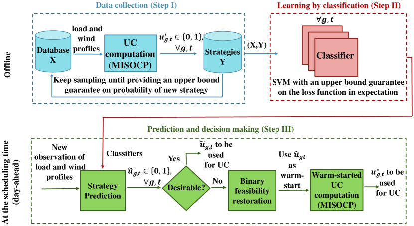
Figure 1: The overall structure of the proposed UC predictor.

The third step uses predicted strategies $\mathbf{y}$. If the underlying strategy is desirable, it is used as a decision for the commitment of conventional units — therefore, no need to solve the UC problem. Otherwise, it is used as a warm start to solve the UC problem. By desirability, we refer to the solution feasibility and prediction loss guarantee. If the prediction is not desirable due to infeasibility, we first recover a feasible solution from the sampled strategies to the infeasible one using the K-nearest neighbor approach, and then use it as a warm start to the original UC problem.

To evaluate the performance of the proposed predictor, we solve the original and warm-started UC problem while assuming there is a computational time limit, e.g., 15 minutes. If the computational time reaches to the limit, we stop the solver and report the results obtained by then, which might be a sub-optimal solution with a high optimality gap. Our thorough out-of-sample simulations show how crucial it is to improve the accuracy of warm starting. By doing so, there is potential to reduce the system cost by solving the UC problem to (near) optimality within a limited computational time frame.

III Step 1: Data Collection

This section explains Step 1 of Fig. 1 (blue part). Suppose we have access to historical forecasts of wind and demand for $T$=$24$ hours of a day, so we can build a feature vector in the form of $\mathbf{x}=[\mathbf{p}^{\rm{W}}_{1},\mathbf{q}^{\rm{W}}_{1},\mathbf{p}^{\rm{D}}_{1},\mathbf{q}^{\rm{D}}_{1},...,\mathbf{p}^{\rm{W}}_{T},\mathbf{q}^{\rm{W}}_{T},\mathbf{p}^{\rm{D}}_{T},\mathbf{q}^{\rm{D}}_{T}]\in\mathbb{R}^{4NT}$, where $N$ is the number of buses. Vectors $\mathbf{p}^{\rm{W}}$, $\mathbf{q}^{\rm{W}}$, $\mathbf{p}^{\rm{D}}$, and $\mathbf{q}^{\rm{D}}$ refer to active and reactive power production (consumption) of wind farms (demands), respectively. For a given hour $t$, we define the active power vector $\mathbf{p}^{\rm{W}}_{t}=\{p^{\rm{W}}_{1t},...,p^{\rm{W}}_{Nt}\}\in\mathbb{R}^{N}$. Vectors $\mathbf{q}_{t}^{\rm{W}}$, $\mathbf{p}_{t}^{\rm{D}}$, and $\mathbf{q}_{t}^{\rm{D}}$ are defined similarly. Having access to historical data of $H$ days provides us with $H$ number of vectors $\mathbf{x}$, collected within the set of vectors $\mathbf{X}=\{\mathbf{x}_{1},...,\mathbf{x}_{h},...,\mathbf{x}_{H}\}$.

Given every vector $\mathbf{x}$, we solve the UC problem as a MISOCP problem, whose formulation is given in the appendix. This gives us the set of strategy vectors $\mathbf{Y}=\{\mathbf{y}_{1}$,$...$,$\mathbf{y}_{h}$,$...$,$\mathbf{y}_{H}\}$. Every strategy vector $\mathbf{y}$ is defined as $\mathbf{y}=[u^{*}_{11}$,$...$,$u^{*}_{MT}]\in\{0,1\}^{MT}$, where $M$ is the number of conventional units, and superscript ^∗ refers to the optimal value obtained by the state-of-the-art solvers, e.g., Gurobi. By this, we eventually collect the set of samples $(\mathbf{X,Y})=\{(\mathbf{x}_{1},\mathbf{y}_{1}),...,(\mathbf{x}_{h},\mathbf{y}_{h}),...,(\mathbf{x}_{H},\mathbf{y}_{H})\}$.

To determine the minimum required number of samples $H$ to be used later for classification, we calculate the probability of encountering a novel strategy $\mathbf{y}_{H+1}$, as in the following theorem outlined in [15]:

Theorem 1.

Given the set of feature vectors $\mathbf{X}$ drawn from an unknown discrete distribution and its corresponding set of strategy vectors $\mathbf{Y}$, the probability of coming across a feature vector $\mathbf{x}_{H+1}$ that corresponds to an unobserved strategy vector $\mathbf{y}_{H+1}$ is

$$\mathbb{P}(\mathbf{y}_{H+1}\notin\mathbf{Y})\leq\frac{H_{1}}{H}+\tau\sqrt{\frac{1}{H}ln(\frac{3}{\epsilon})},$$ (1)

where $H_{1}$ is the number of unique strategies that have been observed only once, $\tau=2\sqrt{2}+\sqrt{3}$, and $1-\epsilon$ is the confidence level of holding (1).

The proof can be directly derived from Theorem 9 of [23]. Considering this theorem, we keep sampling until the bound on the right-hand side of (1) falls below a desired probability guarantee of $\delta$ with a given confidence interval of $1-\epsilon$. This strategy sampling is detailed in Algorithm 1.

Remark: Hereafter, in order to train the classifiers, we convert $y=0$ in our samples to $y=-1$. Therefore, $y_{gt}=-1$ implies that unit $g$ in hour $t$ is off. In contrast, $y_{gt}=1$ still means the unit is on.

IV Step 2: Learning by Binary Classification

This section describes Step 2 of Fig. 1 (red part). Given the training dataset, i.e., the set of samples, $(\mathbf{X,Y})=\{(\mathbf{x}_{1},\mathbf{y}_{1}),...,(\mathbf{x}_{h},\mathbf{y}_{h}),...,(\mathbf{x}_{H},\mathbf{y}_{H})\}$, this step designs a set of binary classifiers to construct the function $\Phi:\mathbb{R}^{4NT}\rightarrow\{-1,1\}^{MT}$ mapping $\mathbf{X}$ to $\mathbf{Y}$. As the number of strategies required to satisfy (1) can increase quickly for some problems, the implementation of a multi-class classification method may impose a heavy computational burden. To overcome it, we make a simplification assumption and develop one binary classifier per each entry of $\mathbf{y}$. This means that for each conventional unit $g$ and time period $t$, we identify a distinct map function $\phi_{gt}:\mathbb{R}^{4NT}\rightarrow\{-1,1\}$. We then gather all of these map functions as $\Phi=\{\phi_{11},...,\phi_{gt},...,\phi_{MT}\}$ to predict the on/off commitment status of conventional units $g=\{1,...,M\}$ at time periods $t=\{1,...,T\}$.

Algorithm 1 Strategy sampling

Given $\delta$ and $\epsilon$
Initialize $H=1$ and $H_{1}=1$
While $\frac{H_{1}}{H}+\tau\sqrt{\frac{1}{H}ln(\frac{3}{\epsilon})}>\delta$

a) Sample $\mathbf{x}_{h}$ and compute $\mathbf{y}_{h}$
b) Update the set of features $\mathbf{X}\leftarrow\mathbf{X}\cup\{\mathbf{x}_{h}\}$
c) Update the set of corresponding strategies $\mathbf{Y}\leftarrow\mathbf{Y}\cup\{\mathbf{y}_{h}\}$
d) if $\mathbf{y}_{h}\notin\mathbf{Y}$ then $H_{1}=H_{1}+1$
e) $H=H+1$
end
Return $\mathbf{X}$ and $\mathbf{Y}$

As already discussed in Section II, we use a SVM technique to develop our binary classifier, providing us with the map functions $\Phi$. We start with a linear SVM, generalize it by adding a regularizer to avoid over-fitting, and finally extend it to a high-dimensional feature space as a non-linear classifier, resulting in a kernelized SVM.

IV-A Linear SVM

Recall we develop one classifier per conventional unit $g$ per hour $t$. Hereafter, we focus on developing a linear SVM for unit $g$ in hour $t$. For notational simplicity, we drop indices $g$ and $t$. For every sample $h=\{1,...,H\}$, the vector $\mathbf{x}_{h}\in\mathbb{R}^{4N}$ and the binary value $y_{h}\in\{-1,1\}$ are input data for the linear SVM classifier. The goal is to divide $H$ samples into two classes by a hyperplane, maximizing the distance between the hyperplane and the nearest point [24, 25]. For that, we solve a linear problem as

$$\min_{\zeta_{h}\geq 0,\mathbf{w},b} \ \ \frac{1}{H}\sum_{h=1}^{H}\zeta_{h}$$ (2a)

s.t. $$y_{h}(\mathbf{w}^{\top}\mathbf{x}_{h}+b)\geq 1-\zeta_{h},\ \forall h,\$$ (2b)

where $\mathbf{w}\in\mathbb{R}^{4N}$ and $b\in\mathbb{R}$ constitute the hyperplane, and $\zeta_{h}\in\mathbb{R}^{+}$ is a slack variable.

Once the optimal values for $\mathbf{w}^{*}$ and $b^{*}$ are obtained by solving (2), any new feature vector $\tilde{\mathbf{x}}$ is classified using the map function

$$\phi(\tilde{\mathbf{x}})=\text{sign}(\mathbf{w}^{{*}^{\top}}\tilde{\mathbf{x}}+b^{*}),$$ (3)

where sign($a$) =1 if $a>0$, and $-1$ if $a<0$. In other words, $\phi(\tilde{\mathbf{x}})$ predicts $\tilde{y}$, such that $\tilde{y}=1$ means the classifier predicts the unit will be on, and $\tilde{y}=-1$ otherwise.

IV-B Reformulating Linear SVM

We reformulate (2) to build up the next section accordingly. The optimal solution to the linear problem (2) would be in one of the corner points, such that in the optimal solution it holds

$$\zeta_{h}=\max\Big{(}0,1-y_{h}(\mathbf{w}^{\top}\mathbf{x}_{h}+b)\Big{)},\ \forall{h}.$$ (4)

Defining the hinge loss function $\mathbf{L}(z,z^{\prime})=\max\big{(}0,1-zz^{\prime}\big{)}$, and replacing $\zeta_{h}$ in (2) with the right hand side of (4), we get

$$\min_{\mathbf{w},b}\ \frac{1}{H}\sum_{h=1}^{H}\mathbf{L}\big{(}y_{h},(\mathbf{w}^{\top}\mathbf{x}_{h}+\!b)\big{)},$$ (5)

which is an unconstrained linear optimization problem, equivalent to (2). If we assume the feature vector $\mathbf{x}_{h}$ follows a probability distribution $\hat{\mathbb{P}}_{H}$, (5) can be written as

$$\min_{\mathbf{w},b}\ \mathbb{E}^{\hat{\mathbb{P}}_{H}}\bigg{[}\mathbf{L}\big{(}y,(\mathbf{w}^{\top}\!\mathbf{x}+b)\big{)}\bigg{]}.$$ (6)

Optimization (6) is an alternative derivation of the linear SVM minimizing the expected risk, where $\mathbb{E}^{\hat{\mathbb{P}}_{H}}[\cdot]$ is the expectation operator with respect to the empirical distribution $\hat{\mathbb{P}}_{H}$ of training dataset with $H$ samples. In the following section, we use (6) to develop a distributionally robust classifier.

IV-C Distributionally robust SVM

An assumption is often made in the current literature that the training data follows a certain distribution, which is also the underlying distribution of the test data. This assumption is often violated in practice. When the underlying probability distribution of the training dataset is unknown, it is desirable to develop a distributionally robust classifier, which is robust to the distributional ambiguity. One approach to develop a distributionally robust classifier is based on Wasserstein distributionally robust optimization. Built upon (6), the distributionally robust SVM writes as

$$\min_{\mathbf{w},b} \ \max_{\mathbb{Q}\in\mathbb{B}_{\rho}(\hat{\mathbb{P}}_{H})}\mathbb{E}^{\mathbb{Q}}\bigg{[}\mathbf{L}\big{(}y,(\mathbf{w}^{\top}\mathbf{x}+b)\big{)}\bigg{]},$$ (7)

where $\mathbb{B}_{\rho}(\hat{\mathbb{P}}_{H})$ denotes the set of distributions whose distance to the empirical distribution $\hat{\mathbb{P}}_{H}$ is lower than or equal to the pre-defined value $\rho\in\mathbb{R}$. Optimization (7) obtains the worst distribution $\mathbb{Q}$ within $\mathbb{B}_{\rho}(\hat{\mathbb{P}}_{H})$, and optimally classifies samples against it. This distributional robustification helps reduce the risk of misclassification and over-fitting in real-world applications.

It has been proven in [26] and [27] that, under certain circumstances, (7) is equivalent to a regularized version of the linear SVM (6). Accordingly, for every $\rho\geq 0$, there exists a value $\lambda\in\mathbb{R}$ such that the distributionally robust SVM is analogous to the regularized SVM. As a result, (7) is equivalently rewritten as

$$\min_{\mathbf{w},\mathbf{b}} \ \frac{1}{H}\sum_{h=1}^{H}\mathbf{L}\big{(}y_{h},(\mathbf{w}^{\top}\mathbf{x}_{h}+b)\big{)}+\lambda\lVert\mathbf{w}\rVert^{2}_{2},$$ (8)

where $\lVert\cdot\rVert_{2}$ is the norm $2$ operator. The first term in (8) is the expected hinge loss, whereas the second term is the regularization term to avoid over-fitting. Note that (8) is an unconstrained quadratic programming (QP) problem.

The resulting distributionally robust SVM offers an upper-bound guarantee on the expected prediction loss function, commonly referred to as an out-of-sample guarantee. Let us consider a test dataset $\{(\tilde{\mathbf{x}}_{1},\tilde{y}_{1}),...,(\tilde{\mathbf{x}}_{h},\tilde{y}_{h}),...,(\tilde{\mathbf{x}}_{\tilde{H}},{\tilde{y}}_{\tilde{H}})\}$ of $\tilde{H}$ samples. Assuming the distribution of the test dataset lies in $\mathbb{B}_{\rho}(\hat{\mathbb{P}}_{H})$, it holds that

$$\frac{1}{\tilde{H}}\sum_{h=1}^{\tilde{H}}\mathbf{L}\big{(}\tilde{y}_{h},(\mathbf{w^{*}}^{\top}\tilde{\mathbf{x}}_{h}+b^{*})\big{)}\leq J(\lambda),$$ (9)

where $J(\lambda)$ is the optimal value of (8).

The takeaway is that the distributionally robust SVM (8) is equivalent to the regularized form of the linear SVM (2), i.e.,

$$\min_{\zeta_{h}\geq 0,\mathbf{w},b} \ \ \frac{1}{H}\sum_{h=1}^{H}\zeta_{h}+\lambda\lVert\mathbf{w}\rVert^{2}_{2}$$ (10a)

s.t. $$y_{h}(\mathbf{w}^{\top}\mathbf{x}_{h}+b)\geq 1-\zeta_{h},\ \forall h.\$$ (10b)

The QP problem (10) can be efficiently solved by replacing $\lambda\lVert\mathbf{w}\rVert^{2}_{2}$ in the objective function by an auxiliary variable $\varrho$ and then adding the constraint $\varrho\geq\lambda\lVert\mathbf{w}\rVert^{2}_{2}$. By doing so, (10) becomes a second-order cone programming (SOCP) problem with a linear objective function.

IV-D Kernelized SVM

By solving either the linear SVM (2) or the distributionally robust SVM (8) or its equivalent regularized SVM (10), we end up in a linear map function $\phi({\mathbf{x}})=\text{sign}(\mathbf{w}^{{*}^{\top}}{\mathbf{x}}+b^{*})$. Aiming to a more efficient classification with a higher degree of freedom, it is desirable to obtain a non-linear map function while preserving the convexity of optimization problems. For this purpose, we use the kernel trick to transform data into a higher dimensional space.

The rationale is to transform the regularized SVM (10) from the Euclidean space to an infinite-dimensional Hilbert space $\mathbb{H}$, obtaining a linear map function there, and transforming it back to the Euclidean space as a non-linear function [25, 28]. It has been discussed in the literature that it is computationally desirable to transform the dual optimization of (10). This dual optimization in the Euclidean space is

$$\max_{\alpha_{h}} \sum_{h}\alpha_{h}-\frac{1}{2}\sum_{k,h}\alpha_{k}\alpha_{h}y_{k}y_{h}\mathbf{x}_{k}\mathbf{x}_{h}$$ (11a)

s.t. $$\sum_{h}y_{h}\alpha_{h}=0$$ (11b)

$$0\leq\alpha_{h}\leq\lambda,\ \forall h,$$ (11c)

where $h=\{1,...,H\}$ and $k=\{1,...,H\}$ are indices for samples. In addition, $\alpha_{h}$ is the dual variable corresponding to (10b). This dual SVM is the Hilbert space [29] is written as

$$\max_{\alpha_{h}} \sum_{h}\alpha_{h}-\frac{1}{2}\sum_{k,h}\alpha_{k}\alpha_{h}y_{k}y_{h}\Psi(\mathbf{x}_{k})\Psi(\mathbf{x}_{h})$$ (12a)

s.t. $${\rm{\eqref{dual_con1}-\eqref{dual_con2}}},$$ (12b)

where the map $\Psi:\mathbb{R}^{4N}\rightarrow\mathbb{H}$ transforms the vectors from the Euclidean to the Hilbert space. The kernel trick states that there are functions $f(\mathbf{x}_{k},\mathbf{x}_{h})$ in the Euclidean space which are equivalent to the dot product $\Psi(\mathbf{x}_{k})\Psi(\mathbf{x}_{h})$ in the Hilbert space. One popular function satisfying such a property is the Gaussian kernel function [30, 31], defined as $f(\mathbf{x}_{k},\mathbf{x}_{h})=e^{-\gamma\lVert\mathbf{x}_{k}-\mathbf{x}_{h}\rVert^{2}_{2}}$, where the parameter $\gamma$ controls the flexibility degree of the hyperplane (tuned by cross-validation). Now, the kernelized SVM (dual form) in the Euclidean space is written as

$$\max_{\alpha_{h}} \sum_{h}\alpha_{h}-\frac{1}{2}\sum_{k,h}\alpha_{k}\alpha_{h}y_{k}y_{h}f(\mathbf{x}_{k},\mathbf{x}_{h})$$ (13a)

s.t. $${\rm{\eqref{dual_con1}-\eqref{dual_con2}}}.$$ (13b)

Now, we convert (13) back to its primal form:

$$\min_{\zeta_{h}\geq 0,\boldsymbol{\beta}} \ \ \frac{1}{H}\sum_{h=1}^{H}\zeta_{h}+\lambda\lVert{\boldsymbol{f}^{\frac{1}{2}}\boldsymbol{\beta}}\rVert^{2}_{2}$$ (14a)

s.t. $$\sum_{k=1}^{H}y_{k}f(\mathbf{x}_{k},\mathbf{x}_{h})\beta_{k}\geq 1-\zeta_{h},\ \forall h,\$$ (14b)

where $\boldsymbol{\beta}\in\mathbb{R}^{H}$ and $\boldsymbol{f}\in\mathbb{R}^{H\times H}$. Similar to (10), optimization (14) is a QP problem, however one can convert it to a SOCP problem by moving the quadratic regularizer from the objective function to constraints.

Once (14) is solved and the optimal value for $\boldsymbol{\beta}^{*}$ is obtained, any new feature vector $\tilde{\mathbf{x}}$ is classified using the map function

$$\phi(\tilde{\mathbf{x}})=\text{sign}\Big{(}\sum_{h=1}^{H}f(\tilde{\mathbf{x}},\mathbf{x}_{h})\beta^{*}_{h}\Big{)},$$ (15)

where the interpretation is the same as that of (3).

IV-E Distributionally Robust Kernelized SVM

The kernelized SVM (14) is equivalent to

$$\min_{\boldsymbol{\beta}} \ \ \frac{1}{H}\sum_{h=1}^{H}\mathbf{L}\Big{(}y_{h},\sum_{k=1}^{H}f(\mathbf{x}_{k},\mathbf{x}_{h})\beta_{k}\Big{)}+\lambda\lVert{\boldsymbol{f}^{\frac{1}{2}}\boldsymbol{\beta}}\rVert^{2}_{2}.$$ (16)

Similar to the discussion for (7), it has been proven in [26] and [27] that the kernelized SVM (16) with the regularization term $\lambda\lVert{\boldsymbol{f}^{\frac{1}{2}}\boldsymbol{\beta}}\rVert^{2}_{2}$, under certain conditions, is equivalent to a distributionally robust kernelized classifier as

$$\min_{\boldsymbol{\beta}} \max_{\mathbb{Q}\in\mathbb{B}_{\rho}(\hat{\mathbb{P}}_{H})}\mathbb{E}^{\mathbb{Q}}\Big{[}\mathbf{L}\Big{(}y,\sum_{h=1}^{H}f(\mathbf{x},\mathbf{x}_{h})\beta_{h}\Big{)}\Big{]}.$$ (17)

Similar to (9), it holds that

$$\frac{1}{\tilde{H}}\sum_{k=1}^{\tilde{H}}\mathbf{L}\Big{(}\tilde{y}_{k},\sum_{h=1}^{H}f(\tilde{\mathbf{x}}_{k},\mathbf{x}_{h})\beta^{*}_{h}\Big{)}\leq J^{\prime}(\lambda),$$ (18)

where $J^{\prime}(\lambda)$ is the optimal value of (16).

A summary of various binary classifications is given in Table I.

Table I: Summary of various binary classifications

Type of	Without	With regularization
Classification	regularization	(distributionally robust)
Linear SVM	(2) or (10) with $\lambda=0$	(10)
Kernelized SVM	(14) with $\lambda=0$	(14)

V Step 3: Prediction and Decision Making

This section explains Step 3 of Fig. 1 (green part). The map functions (3) for the linear SVM and (15) for the kernelized SVM enable us to predict the commitment decision $\tilde{\mathbf{y}}$ of conventional units, having features $\tilde{\mathbf{x}}$ as the input data. To guarantee the prediction performance, we present a confidence level for inaccuracy of predicted $\tilde{\mathbf{y}}$ based on the concept of distributionally robust classification. This guarantee provides an upper bound on the prediction loss in expectation, which is already mentioned in (9) and (18). Note that we here consider the hinge loss function to measure the accuracy of prediction.

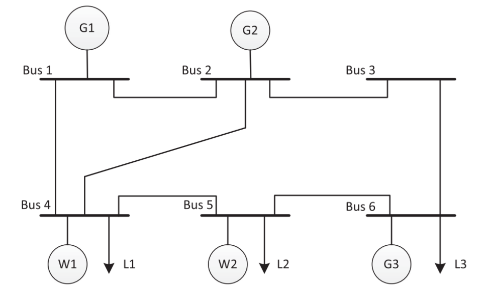
Figure 2: The IEEE $6$-bus test system with three conventional units $\rm{G}1$-$\rm{G}3$, two wind farms $\rm{W}1$-$\rm{W}2$, and three loads $\rm{L}1$-$\rm{L}3$.

Figure 3: The number of missclassified samples and CPU time for SVM classifiers using $50$, $500$, and $5,000$ training samples and $1,000$ test samples.

Once $\tilde{\mathbf{y}}$ predicted, we check the feasibility and the upper bound guarantee. If the prediction is feasible and the guarantee is desirable, the prediction is directly adopted as the commitment decision for conventional units. Otherwise, we use $\tilde{\mathbf{y}}$ as a warm start to the MISOCP solver built upon a branch-and-bound algorithm. Note that for this, we convert back $\tilde{y}_{gt}=-1$ to $\tilde{y}_{gt}=0$, indicating the corresponding unit is off. The branch-and-bound algorithm uses the warm start as an initial solution. By that, it uses the warm start as a bound to eliminate parts of the search space that cannot produce a better solution and therefore focus on the rest of search space. This is particularly useful when the MISOCP problem has a large number of variables, and the solution space is vast. We find a trade-off between prediction quality and computational time to determine how much mixed-integer solvers can benefit from utilizing the predicted $\tilde{\mathbf{y}}$ as a warm start.

As mentioned earlier, predicted $\tilde{\mathbf{y}}$ to be used as a warm start might be infeasible for the MISOCP problem. If it is the case, we find a close feasible solution among the sampled strategies to the infeasible one by using the K-nearest neighbor algorithm [32] to recover a feasible solution. Furthermore, in order to guarantee that there is always a feasible solution to the UC problem, we also take corrective measures like load shedding and renewable power curtailment into consideration.

VI Experimental results

We provide two case studies based on the IEEE $6$-bus and $118$-bus test systems. We solve the optimization problems in Python using scikit-learn API and in Matlab using the YALMIP toolbox with Gurobi solver $8.1.1$ on a $16$ GB RAM personal computer clocking at $3.1$ GHZ. All source codes are publicly available in [33].

VI-A IEEE 6-bus test system

This stylized system includes $3$ conventional units, $2$ wind farms, and $3$ loads, as shown in Fig. 2. The technical data for conventional units and transmission lines is given in [33]. For simplicity in this stylized case, we assume that loads are deterministic and that two wind farms only have stochastic generation. Additionally, we assume an identical shape for daily wind power generation profile across different samples — the only varying factor is their generation level. As such, we end up in two features only, i.e., the production level of two wind farms. Wind and load data is provided in [33].

Training data

We utilize three distinct sets of training data for our analysis, which contain $50$, $500$, and $5,000$ samples, respectively. Recall for generating each sample $(\mathbf{x},\mathbf{y})$, we solve the MISOCP problem given in the appendix with the feature vector $\mathbf{x}$ as the input data, and compute commitments $\mathbf{y}$. Based on Algorithm 1 in Section III, given $\epsilon=0.10$, these number of training samples provide a desired probability guarantee of $\delta=1$, $\delta=0.40$, and $\delta=0.18$, respectively. This means that, if one provides further samples beyond $50$, $500$, and $5,000$ training samples, the maximum probability of observing a new strategy with the confidence level of $90\%$ is $100\%$, $40\%$, and $18\%$, respectively. Having samples $(\mathbf{x},\mathbf{y})$ as inputs data, we solve the linear or conic optimization problems for SVM classifiers (see Table I), and obtain map functions (3) for the linear SVM and (15) for the kernelized SVM.

Testing data

We use a dataset containing $1,000$ samples in the form of $(\tilde{\mathbf{x}},\tilde{\mathbf{y}})$, which are different than training samples. We use the map functions (3) and (15) to predict $\tilde{\mathbf{y}}$, to be used either as a commitment decision or to serve for warm starting.

Cross-validation for kernel function and regularizer

We have used a cross-validation approach to tune the parameter $\gamma$ in the Gaussian kernel function. To so do, we split $1,000$ testing samples into $4$ equally sized subsets and then training the model on $3$ subsets, while validating its performance on the remaining subset. This process is repeated $4$ times, with each subset being used as the validation set once, and the other $3$ subsets being used for training. The performance metric used is the expected hinge loss of validation instances. Similarly, we regularize both linear and kernelized SVM classifiers by determining a value for $\lambda$, obtained by cross-validation too.

Classification results

Let us first explore how successful the map functions (3) and (15) are in the prediction of the correct commitments. Fig. 3 shows classification boundaries for the commitment of arbitrarily selected conventional unit $\rm{G}3$ in a certain hour. For every plot, the two axes are wind production of two farms (two available features). Based on classification results, it is predicted $\rm{G}3$ to be off in the blue area and to be on in the brown area. The blue and brown circles indicate the true commitment, obtained by solving the MISOCP problem in the appendix. If a blue (brown) circle is located in the blue (brown) area, it shows that the prediction is correct, otherwise it is a misclassification. This figure includes $12$ plots, where those in the first, second, and third rows correspond to cases where the number of training samples is $50$, $500$, and $5,000$, respectively. The plots in the first two columns pertain to the training stage, where those plots in the third and fourth columns show the testing results with $1,000$ samples. Under each plot, the number of misclassified samples and the corresponding computational time (in the training stage) are reported.

One main observation is that the kernelized SVM outperforms the linear one in terms of the number of misclassified samples in both training and testing stages. For example, in the case with $500$ training samples, the kernelized SVM in the training stage (plot $6$) has only $3$ out of $500$ samples wrongly classified, whereas it is $41$ for the linear SVM (plot $5$). Similarly, in the testing stage, the kernelized SVM misclassified $28$ out of $1,000$ samples (plot $8$), while it is $96$ samples for the linear SVM (plot $7$). There is a similar observation in the case with $5,000$ training samples, i.e., plots $9$-$12$. This has been expected as the kernelized SVM offers a higher degree of freedom when determining a map function, resulting in nonlinear boundaries between blue and brown areas. The interesting point is that the computational time for training the kernelized SVM is lower than the linear one, making it even a more appealing choice. Another interesting observation is that by increasing the number of training samples from $500$ to $5,000$, the kernelized SVM exhibits a more successful performance in the testing stage (reduced misclassified samples from $28$ in plot $8$ to $14$ in plot $12$). However, it is not the case for the linear SVM (see plots $7$ and $11$).

Bias analysis and performance guarantee

We first start with a bias analysis in terms of the similarity of training and test datasets. We keep the previous training dataset with $5,000$ samples. However, we generate two different test datasets, each with $1,000$ samples, one is more similar to the training dataset, while the other one is less similar. We use the $2$-Wasserstein metric to measure the distance of training and test datasets. The similar test dataset, so called biased test dataset, has a distance of $0.05$ to the training samples. In contrast, the other one, so called unbiased test dataset, has a comparatively higher distance of $0.20$. We then exploit the kernelized SVM classifier (14) including a regularization term.

For all three conventional units over $24$ hours, Fig. 4 reports the optimal value of the expected hinge loss of the kernelized SVM classifier in both training and testing stages. For the training dataset, recall that the expected hinge loss is equal to (16) in the optimal point, whereas for the test datasets, it is computed as the left-hand side of (18). Owed to the regularization weight $\lambda$ carefully tuned by cross validation, the expected hinge loss in the unbiased test dataset is lower than that in the biased one, which is desirable. In addition, the expected hinge loss in both biased and unbiased test datasets is lower than that of the training dataset, validating the performance guarantee (18) is obtained.

VI-B IEEE 118-bus test system

We apply the proposed UC predictor to the IEEE $118$-bus test system, including $19$ conventional units, $2$ wind farms, $91$ loads, and $186$ transmission lines. Our main focus is on the potential improvement in the computational performance. Furthermore, we investigate the potential cost saving by improving the optimality gap.

Data preparation

We use a dataset comprising of $5,000$ samples for training and $1,000$ samples for testing. The features that we consider here include the power generation of wind farms as well as the load in all buses over $24$ hours. Therefore, each classifier for unit $g$ and hour $t$ has access to $93$ features. Note that we assume all loads and wind farms adhere to a fixed power factor. Additionally, we assume an identical daily load and wind power generation profile across various samples. Times series for daily load and wind power generation are given in [33]. For each sample, we solve the MISOCP problem (see appendix), including $2,592$ binary variables, $13,920$ continuous variables, and $55,464$ linear and conic constraints. With a confidence level of $1-\epsilon=0.90$, Algorithm 1 in Section III validates a probability guarantee of $\delta=0.12$ to observe a new strategy. This means, with the confidence level of $90$%, there is a maximum probability of $12$% to observe a new strategy if further training samples are provided. Similar to the previous case study, we tune the parameters for regularization and Gaussian kernel function using a cross-validation approach with $4$ equally sized subsets.

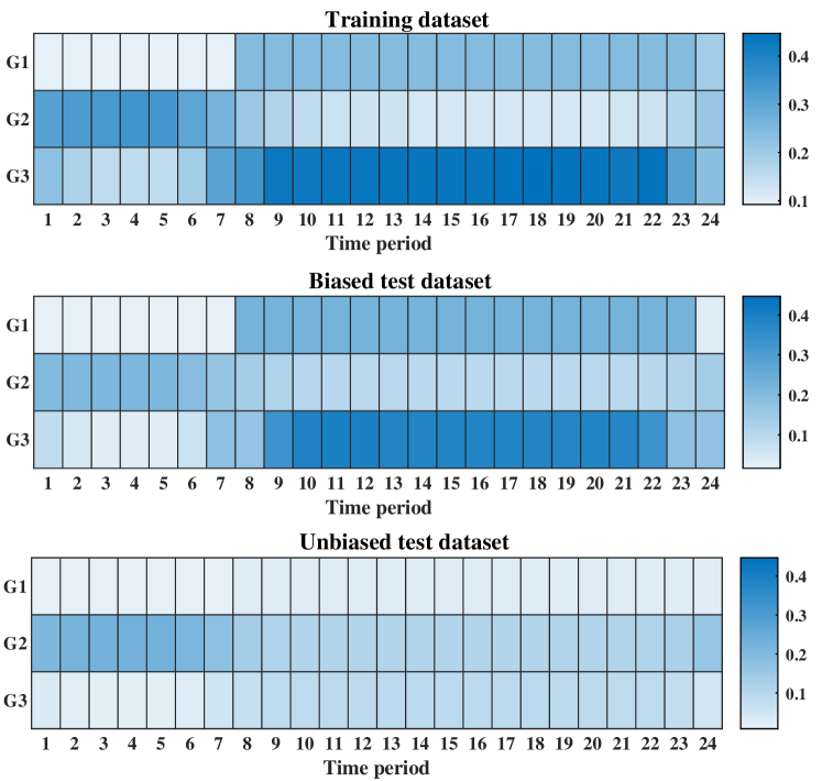
Figure 4: The expected hinge loss of the kernelized SVM classifier, for every unit and hour, in the training and testing stages (with biased and unbiased test data).

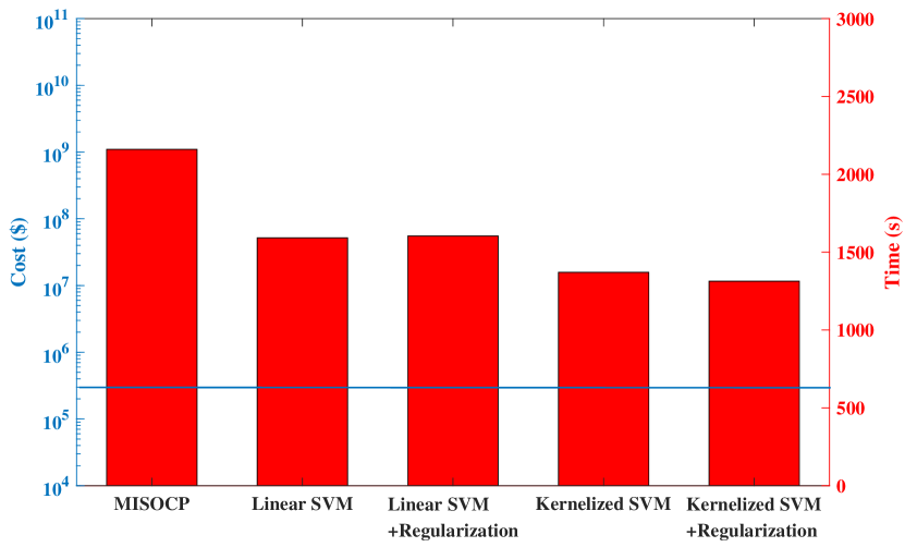
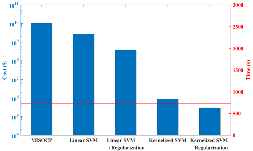
Figure 5: Out-of-sample performance: Average system cost and average computational time for solving the UC problem, solved by the MISOCP solver without (bar 1) or with warm start (bars 2-5). If warmly started, it is initiated by the prediction of classifiers. The right plot enforces a computational time limit of $700$ seconds, and shows the system cost obtained in such a limited period. The left plot shows the computational time when no limit is enforced.

Implementation

We train a classifier for every unit and hour. If the predicted strategy $\tilde{\mathbf{y}}$ is desirable, we can directly use it to determine the commitment of conventional units, but we must still verify that the minimum up- and down-time requirements are satisfied. Otherwise, if the predicted strategy $\tilde{\mathbf{y}}$ is not desirable, we leverage it as a warm start for the Gurobi solver and explore whether it speeds up the computational time to solve the UC problem, i.e., the MISOCP problem in the appendix. If $\tilde{\mathbf{y}}$ is not binary feasible, we use the K-nearest neighbor technique to find a feasible strategy that is as close as possible to the predicted strategy. The K-nearest neighbor technique searches among the strategies sampled for the training dataset. The distance between strategies can be measured as $\lVert\widehat{\mathbf{y}}-\tilde{\mathbf{y}}\rVert$, where $\tilde{\mathbf{y}}$ is the predicted strategy and $\widehat{\mathbf{y}}$ is the closest feasible strategy, respectively.

Evaluation

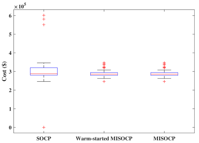
Figure 6: The median and the $25$th and $75$th percentiles of the out-of-sample system cost obtained by solving the UC problem. First bar: UC problem with fixed predictions (binary variables) resulting in a second-order cone programming (SOCP) problem. Second and third bars: UC problem as a MISOCP problem with and without warm start.

In the setting that we use the prediction as a warm start to the MISOCP problem, it is likely to end up in a sub-optimal prediction, but it may still help reduce the computational time. Hereafter, we acknowledge a UC prediction to be effective if it enhances the computational performance of the UC solver. Therefore, our measurement for the prediction effectiveness is to what extent it reduces the computational time. In the following, we examine two scenarios: in Scenario I, the system operator has a limit for the computational time which cannot be exceeded. This implies that the UC problem may not be solved to optimality if the computational time reaches to its limit. In Scenario II, there is not such a limit, and therefore the UC problem can be solved to optimality.

Now, we answer two questions: (i) What is the least possible difference between the optimal strategies $\mathbf{y}^{*}$ and the predicted ones $\tilde{\mathbf{y}}$ under Scenario I (with time limit)? (ii) How quickly can we obtain the optimal strategies $\mathbf{y}^{*}$ under Scenario II (no time limit) with warm starting? To answer these two questions, we train four different classifiers, namely the linear SVM (with and without regularization) and the kernelized SVM (with and without regularization). We then compare the UC results with and without using warm starts — in the case of warm start, the classifiers provide the initial solution.

In the following, with or without warm start, we solve the UC problem $1,000$ times (each time with a different test dataset), and report the average out-of-sample system cost and the average computational time. By the out-of-sample system cost, we refer to the total generation and start-up cost of the system, as formulated in the objective function (19a) of the UC problem in the appendix.

The right plot of Fig. 5 answers the first question under scenario I, where the computational time limit of $700$ seconds has been enforced. This implies when the computational time has reached to this limit, we stopped the solver, and reported the system cost. One can expect that this cost is significantly high if the solver has not managed to find a solution with a low optimality gap in the limited computational period. The right plot of Fig. 5 shows that the warmly started MISOCP problem initiated by the predictions of the kernelized SVM with regularization (last bar) has been solved effectively, resulting in the lowest system cost on average. On the contrary, the MISOCP solver without warm start (first bar) is very slow, such that it could not solve the UC problem effectively in $700$ seconds, yielding a high optimality gap, and thereby a significant system cost. The MISOCP solver warmly started by the predictions of other classifiers exhibits a performance in between. In general, this plot concludes that the kernelized SVM provides more effective warm starts than the linear one.

The left plot of Fig. 5 answers the second question, under scenario II where there is no computational time limit. The MISOCP solver has obtained the same UC solution irrespective of warm or cold start. However, the computational time is significantly higher without warm start. The kernelized SVM with regularization is again the best choice for predicting an effective warm start, reducing the computational time by an average factor of $1.7$, compared to a case with no warm start.

We now evaluate the out-of-sample system cost if we trust in predicted strategies $\tilde{\mathbf{y}}$ and directly use them as commitment decisions of conventional units. We fix the binary variables in the UC problem to those predictions, resulting in a SOCP problem. Fig. 6 shows the median and the $25$th and $75$th percentiles of the out-of-sample system cost when we solve the SOCP problem with fixed binary variables, and compares it to those results of MISOCP without or with warm start (by the kernelized SVM with regularization). It has been observed that the system cost when fixing binary variables is $5$% higher than that of the MISOCP problem, but it is $4.5$ times faster in terms of computational time than the MISOCP problem without warm start, and $2.4$ times faster than the same problem with warm start.

VII Conclusion

This paper showed that, if the system operators have restricted by computational time limits to solve the UC problem, there is a high potential to use SVM-based classification methods to predict commitment decisions of conventional units. As a pragmatic solution, these predictions can be used as a warm start to considerably speed up the mixed-integer optimization solvers, without compromising the optimality. We showed that it is possible to properly regularize the SVM classifiers in a way that it provides an out-of-sample performance guarantee. In addition, this paper discussed how many training samples are needed to get an insight into the probability of having unseen strategies. This paper concluded that the kernelized SVM with a proper regularization (tuned by cross validation) outperforms the linear SVM, and can help the system operators to ease their computational burden.

This paper has developed one classifier per conventional unit per hour. This overlooks the potential spatio-temporal correlations, which could be very useful information when training the classifiers. It is of interest to develop such correlation-aware classifiers, exploring to what extent it may provide more effective predictions (e.g., for warm start) and helps to further reduce the computational time. Another future direction is to explore the performance of classifiers in non-stationary environments, where one may not learn much for old data.

Appendix: MISOCP Formulation for UC Problem

Notation: We consider a power grid consisting of $N$ buses, $L$ transmission lines, and $M$ conventional units. For every hour $t$, the set of continuous variables contains active power generation of conventional units $\mathbf{p}^{\rm{G}}_{t}=\{p^{\rm{G}}_{1t},...,p^{\rm{G}}_{gt},...,p^{\rm{G}}_{Mt}\}\in\mathbb{R}^{M}$, reactive power generation of conventional units $\mathbf{q}^{\rm{G}}_{t}=\{q^{\rm{G}}_{1t},...,q^{\rm{G}}_{gt},...,q^{\rm{G}}_{Mt}\}\in\mathbb{R}^{M}$, nodal voltage magnitudes $\boldsymbol{\nu}_{t}=\{\nu_{1t},...,\nu_{it},...,\nu_{Nt}\}\in\mathbb{R}^{N}$, nodal voltage angles $\boldsymbol{\theta}_{t}=\{\theta_{1t},...,\theta_{it},...,\theta_{Nt}\}\in\mathbb{R}^{N}$, and apparent power flow of transmission lines $\mathbf{s}_{t}=\{s_{1t},...,s_{lt},...,s_{Lt}\}\in\mathbb{R}^{L}$. In addition, the set of binary variables includes on/off commitment of conventional units $\mathbf{u}_{t}=\{u_{1t},...,u_{gt},...,u_{Mt}\}\in\{0,1\}^{M}$ and their start-up status $\mathbf{v}_{t}=\{v_{1t},...,v_{gt},...,v_{Mt}\}\in\{0,1\}^{M}$.

We now define parameters. For each conventional unit $g$, parameters $\overline{p}_{g}/\underline{p}_{g}$ and $\overline{q}_{g}/\underline{q}_{g}$ indicate the maximum/minimum active and reactive power generation limits, respectively. Parameters $\overline{r}_{g}/\underline{r}_{g}$ denote the maximum ramp-up and ramp-down capabilities, whereas $\tilde{r}_{g}$ gives the ramp-rate capability in start-up and shut-down hours. Parameter $\underline{v}_{g}$ gives the minimum up- and down-time, respectively. In addition, $\mathbf{c}^{P}=\{c^{P}_{1},...,c^{P}_{g},...,c^{P}_{M}\}\in\mathbb{R}^{M}$ and $\mathbf{c}^{S}=\{c^{S}_{1},...,c^{S}_{g},...,c^{S}_{M}\}\in\mathbb{R}^{M}$ give the production and start-up costs of conventional units, respectively. For each transmission line $l$ connecting bus $i$ to bus $j$, $G_{ij}$ and $B_{ij}$ denote the real and imaginary parts of the bus admittance matrix, respectively. In addition, $B^{\rm{sh}}_{ij}$ represents the reactive shunt element, considering a $\pi$-model for transmission lines. The apparent power capacity of line $l$ is given by $\overline{s}_{l}$. For each bus $i$, $\overline{\nu}_{i}/\underline{\nu}_{i}$ gives the maximum/minimum voltage magnitude. Parameters $\mathbf{p}^{\rm{W}}_{t}=\{p^{\rm{W}}_{1t},...,p^{\rm{W}}_{it},...,p^{\rm{W}}_{Nt}\}\in\mathbb{R}^{N}$ and $\mathbf{q}^{\rm{W}}_{t}=\{q^{\rm{W}}_{1t},...,q^{\rm{W}}_{it},...,q^{\rm{W}}_{Nt}\}\in\mathbb{R}^{N}$ denote active and reactive power generation of wind farms, respectively. Finally, $\mathbf{p}^{\rm{D}}_{t}=\{p^{\rm{D}}_{1t},...,p^{\rm{D}}_{it},...,p^{\rm{D}}_{Nt}\}\in\mathbb{R}^{N}$ and $\mathbf{q}^{\rm{D}}_{t}=\{q^{\rm{D}}_{1t},...,q^{\rm{D}}_{it},...,q^{\rm{D}}_{Nt}\}\in\mathbb{R}^{N}$ represent nodal active and reactive power consumptions, respectively.

The original AC unit commitment problem reads as

$$\min_{\mathbf{p},\mathbf{q},\mathbf{u},\mathbf{v},\boldsymbol{\nu},\boldsymbol{\theta}}\ \ \sum_{t}\mathbf{p}^{\rm{G}}_{t}(\mathbf{c}^{P})^{\top}+\mathbf{v}_{t}(\mathbf{c}^{S})^{\top}$$ (19a)

$$-\!u_{g(t-1)}\!+\!u_{gt}-u_{g\tau}\!\leq\!0,\forall\tau\!\in\!\{t,...,\!\overline{v}_{g}+t\!-\!1\},\forall g,t$$ (19b)

$$\;u_{g(t-1)}-u_{gt}+u_{g\tau}\leq\!1,\forall\tau\!\in\!\{t,...,\!\underline{v}_{g}+t\!-\!1\},\forall g,t$$ (19c)

$$-u_{g(t-1)}+u_{gt}-v_{gt}\leq 0,\enspace\forall g,t$$ (19d)

$$u_{gt}\underline{p}_{g}\leq p^{\rm{G}}_{gt}\leq\overline{p}_{g}u_{gt},\enspace\forall g,t$$ (19e)

$$u_{gt}\underline{q}_{g}\leq q^{\rm{G}}_{gt}\leq\overline{q}_{g}u_{gt},\enspace\forall g,t$$ (19f)

$$p^{\rm{G}}_{gt}-p^{\rm{G}}_{g(t-1)}\leq\overline{r}_{g}u_{g(t-1)}+\tilde{r}_{g}(1-u_{g(t-1)}),\enspace\forall g,t$$ (19g)

$$p^{\rm{G}}_{g(t-1)}-p^{\rm{G}}_{gt}\leq\underline{r}_{g}u_{gt}+\tilde{r}_{g}(1-u_{gt}),\enspace\forall g,t$$ (19h)

$$\sum_{g\in\Gamma(i)}\!\!p^{\rm{G}}_{gt}+p^{\rm{W}}_{it}-p^{\rm{D}}_{it}=G_{ii}\nu_{it}^{2}+\!\sum_{j\in\Lambda(i)}\!\!\!\nu_{it}\nu_{jt}$$

$$\hskip 42.67912pt\Big{(}G_{ij}\cos(\theta_{it}\!-\!\theta_{jt})\!\!+\!B_{ij}\sin(\theta_{it}\!-\!\theta_{jt})\Big{)},\forall i,t\!$$ (19i)

$$\sum_{g\in\Gamma(i)}\!\!q^{\rm{G}}_{gt}+q^{\rm{W}}_{it}-q^{\rm{D}}_{it}=-B_{ii}\nu_{it}^{2}+\!\sum_{j\in\Lambda(i)}\!\!\!\nu_{it}\nu_{jt}$$

$$\hskip 42.67912pt\Big{(}G_{ij}\sin(\theta_{it}\!-\!\theta_{jt})\!\!-\!B_{ij}\cos(\theta_{it}\!-\!\theta_{jt})\Big{)},\forall i,t$$ (19j)

$$s^{2}_{lt}=\Big{(}\!-G_{ij}\nu_{it}^{2}\!+\!G_{ij}\nu_{it}\nu_{jt}\cos(\theta_{it}\!-\!\theta_{jt})\!$$

$$\hskip 14.22636pt+\!B_{ij}\nu_{it}\nu_{jt}\sin(\theta_{it}\!-\!\theta_{jt})\Big{)}^{2}+\Big{(}\!(B_{ij}-B_{ij}^{\rm{sh}})\nu_{it}^{2}\!$$

$$\hskip 14.22636pt-\!B_{ij}\nu_{it}\nu_{jt}\cos(\theta_{it}\!-\!\theta_{jt})\!+\!G_{ij}\nu_{it}\nu_{jt}\sin(\theta_{it}\!-\!\theta_{jt})\Big{)}^{2},$$

$$\hskip 170.71652pt\forall l\in(i,j),t$$ (19k)

$$s^{2}_{lt}\leq\overline{s}_{l}^{2},\enspace\forall l\in(i,j),t$$ (19l)

$$\underline{\nu}_{i}\leq\nu_{it}\leq\overline{\nu}_{i},\enspace\forall i,t$$ (19m)

$$\theta_{ref,t}=0,\enspace\forall t$$ (19n)

$$\textbf{u}_{t},\textbf{v}_{t}\in\{0,1\},\enspace\forall t.$$ (19o)

The objective function (19a) minimizes the total production and start-up costs of conventional units. Constraints (19b)-(19c) restrict the minimum up- and down-time, whereas (19d) determines the state transition of conventional units. Capacity and ramping limits of conventional units are enforced by (19e)-(19h). Constraints (19i)-(19j) represent the nodal active and reactive power balance, where $\Gamma(i)$ and $\Lambda(i)$ denote the set of conventional units connected to bus $i$ and the set of adjacent buses to $i$, respectively. Constraint (19k) determines the apparent power flow in line $(i,j)$, constrained by (19l). Constraint (19m) limits the voltage magnitudes. Constraint (19n) sets voltage angle of the reference bus to zero. Finally, (19o) declares the binary variables.

This AC unit commitment includes non-convex constraints (19i)-(19k), as they are quadratic equality constraints. For the convexification of those constraints, the current literature [34] suggests defining new variables for each bus $i$ as $w_{it}=\nu_{it}^{2}$ and for each line $(i,j)$ as $e_{ijt}=\nu_{it}\nu_{jt}\cos(\theta_{it}-\theta_{jt})$ and $f_{ijt}=-\nu_{it}\nu_{jt}\sin(\theta_{it}-\theta_{jt})$. This lets replace (19i)-(19l) by

$$\sum_{g\in\Gamma(i)}\!\!\!p^{\rm{G}}_{gt}\!+\!p^{\rm{W}}_{it}\!\!-\!p^{\rm{D}}_{it}\!=$$

$$\hskip 56.9055pt\!G_{ii}\nu_{it}\!+\!\!\!\!\sum_{j\in\Lambda(i)}\!\!\!(G_{ij}e_{ijt}\!\!-\!\!B_{ij}f_{ijt}),\forall i,\!t$$ (20a)

$$\sum_{g\in\Gamma(i)}\!\!\!q^{\rm{G}}_{gt}\!+\!q^{\rm{W}}_{it}\!\!-\!q^{\rm{D}}_{it}\!=$$

$$\hskip 56.9055pt\!-B_{ii}\nu_{it}\!-\!\!\!\!\!\!\sum_{j\in\Lambda(i)}\!\!\!(B_{ij}e_{ijt}\!\!+\!\!G_{ij}f_{ijt}),\forall i,\!t\!$$ (20b)

$$\Big{(}\!-G_{ij}\nu_{it}\!+\!G_{ij}e_{ijt}-\!B_{ij}f_{ijt}\Big{)}^{2}+\!\!\Big{(}\!(B_{ij}\!-\!B_{ij}^{\rm{sh}})\nu_{it}\!$$

$$\hskip 45.5244pt-\!B_{ij}e_{ijt}\!-\!G_{ij}f_{ijt}\Big{)}^{2}\!\!\!\leq\!\overline{s}_{l}^{2},\forall l\!\in\!(i,j),\!t$$ (20c)

$$0=e_{ijt}^{2}+f_{ijt}^{2}-\nu_{it}\nu_{jt},\forall i,j,t$$ (20d)

$$0=\theta_{jt}-\theta_{it}-{\rm{atan}}(\frac{f_{ijt}}{e_{ijt}}),\forall i,j,t$$ (20e)

$$\underline{v}_{i}^{2}\leq\nu_{it}\leq\overline{v}_{i}^{2},\forall i,t$$ (20f)

$$-\overline{v}_{i}\overline{v}_{j}\leq e_{ijt},f_{ijt}\leq\overline{v}_{i}\overline{v}_{j},\forall i,j,t.$$ (20g)

Now, the original formulation converts to (19a)-(19h), (19m)-(19o), (20a)-(20g), which is still non-convex. However, it can be relaxed to a mixed-integer second-order cone optimization by omitting (20e) and relaxing (20d) as

$$e_{ijt}^{2}+f_{ijt}^{2}\leq\nu_{it}\nu_{jt},\forall i,j,t.$$ (21)

The resulting MISOCP problem is (19a)-(19h), (19m)-(19o), (20a)-(20c), (20f)-(20g) and (21), which is used to solve the UC problem in this paper.

References

- [1] M. F. Anjos and A. J. Conejo, “Unit commitment in electric energy systems,” Foundations and Trends® in Electric Energy Systems, vol. 1, no. 4, pp. 220–310, 2017.
- [2] B. F. Hobbs, M. H. Rothkopf, R. P. O’Neill, and H.-p. Chao, The next generation of electric power unit commitment models. Springer Science & Business Media, 2006, vol. 36.
- [3] A. Castillo, C. Laird, C. A. Silva-Monroy, J.-P. Watson, and R. P. O’Neill, “The unit commitment problem with AC optimal power flow constraints,” IEEE Trans. Power Syst., vol. 31, no. 6, pp. 4853–4866, 2016.
- [4] D. A. Tejada-Arango, P. Sánchez-Martın, and A. Ramos, “Security constrained unit commitment using line outage distribution factors,” IEEE Trans. Power Syst., vol. 33, no. 1, pp. 329–337, 2017.
- [5] C. Coffrin and P. Van Hentenryck, “A linear-programming approximation of AC power flows,” INFORMS J. Comput., vol. 26, no. 4, pp. 718–734, 2014.
- [6] R. Madani, M. Ashraphijuo, and J. Lavaei, “Promises of conic relaxation for contingency-constrained optimal power flow problem,” IEEE Trans. Power Syst., vol. 31, no. 2, pp. 1297–1307, 2015.
- [7] C. Coffrin, H. L. Hijazi, and P. Van Hentenryck, “Strengthening the SDP relaxation of AC power flows with convex envelopes, bound tightening, and valid inequalities,” IEEE Trans. Power Syst., vol. 32, no. 5, pp. 3549–3558, 2016.
- [8] S. Atakan, G. Lulli, and S. Sen, “A state transition MIP formulation for the unit commitment problem,” IEEE Trans. Power Syst., vol. 33, no. 1, pp. 736–748, 2017.
- [9] G. Morales-España, J. M. Latorre, and A. Ramos, “Tight and compact milp formulation for the thermal unit commitment problem,” IEEE Trans. Power Syst., vol. 28, no. 4, pp. 4897–4908, 2013.
- [10] J. Ostrowski, M. F. Anjos, and A. Vannelli, “Tight mixed integer linear programming formulations for the unit commitment problem,” IEEE Trans. Power Syst., vol. 27, no. 1, pp. 39–46, 2011.
- [11] D. Rajan and S. Takriti, “Minimum up/down polytopes of the unit commitment problem with start-up costs,” IBM Res. Rep, vol. 23628, pp. 1–14, 2005.
- [12] D. Bertsimas and C. W. Kim, “A prescriptive machine learning approach to mixed-integer convex optimization,” INFORMS J. Comput., 2023, to be published.
- [13] F. Fioretto, T. W. Mak, and P. Van Hentenryck, “Predicting AC optimal power flows: Combining deep learning and Lagrangian dual methods,” in Proceedings of the AAAI Conference on Artificial Intelligence, vol. 34, 2020, pp. 630–637.
- [14] W. Chen, S. Park, M. Tanneau, and P. Van Hentenryck, “Learning optimization proxies for large-scale security-constrained economic dispatch,” Electr. Power Syst. Res., vol. 213, p. 108566, 2022.
- [15] D. Bertsimas and B. Stellato, “Online mixed-integer optimization in milliseconds,” INFORMS J. Comput., vol. 34, no. 4, p. 2229–2248, 2022.
- [16] L. Roald and D. Molzahn, “Implied constraint satisfaction in power system optimization: The impacts of load variations,” in Annual Allerton Conference on Communication, Control, and Computing (Allerton). IEEE, 2019, pp. 308–315.
- [17] D. Deka and S. Misra, “Learning for DC-OPF: Classifying active sets using neural nets,” in IEEE Milan PowerTech, 2019, pp. 1–6.
- [18] S. Misra, L. Roald, and Y. Ng, “Learning for constrained optimization: Identifying optimal active constraint sets,” INFORMS J. Comput., vol. 34, no. 1, pp. 463–480, 2022.
- [19] Á. S. Xavier, F. Qiu, and S. Ahmed, “Learning to solve large-scale security-constrained unit commitment problems,” INFORMS J. Comput., vol. 33, no. 2, pp. 739–756, 2021.
- [20] K. Baker, “Learning warm-start points for AC optimal power flow,” in IEEE 29th International Workshop on Machine Learning for Signal Processing (MLSP). IEEE, 2019, pp. 1–6.
- [21] T. Falconer and L. Mones, “Leveraging power grid topology in machine learning assisted optimal power flow,” IEEE Trans. Power Syst., vol. 38, no. 3, pp. 2234–2246, 2023.
- [22] F. Zohrizadeh, C. Josz, M. Jin, R. Madani, J. Lavaei, and S. Sojoudi, “A survey on conic relaxations of optimal power flow problem,” Eur. J. Oper. Res., vol. 287, no. 2, pp. 391–409, 2020.
- [23] D. A. McAllester and R. E. Schapire, “On the convergence rate of good-turing estimators.” in COLT, 2000, pp. 1–6.
- [24] E. Alpaydin, Introduction to machine learning. MIT press, 2020.
- [25] T. Hastie, R. Tibshirani, J. H. Friedman, and J. H. Friedman, The elements of statistical learning: data mining, inference, and prediction. Springer, 2009, vol. 2.
- [26] S. Shafieezadeh-Abadeh, D. Kuhn, and P. M. Esfahani, “Regularization via mass transportation,” Journal of Machine Learning Research, vol. 20, no. 103, pp. 1–68, 2019.
- [27] D. Kuhn, P. M. Esfahani, V. A. Nguyen, and S. Shafieezadeh-Abadeh, “Wasserstein distributionally robust optimization: Theory and applications in machine learning,” in Operations Research & Management Science in the Age of Analytics, 2019, pp. 130–166.
- [28] C. M. Bishop and N. M. Nasrabadi, Pattern recognition and machine learning. Springer, 2006, vol. 4, no. 4.
- [29] V. N. Vapnik, The nature of statistical learning theory. Springer, 1999.
- [30] K.-R. Muller, S. Mika, G. Ratsch, K. Tsuda, and B. Scholkopf, “An introduction to kernel-based learning algorithms,” IEEE Transactions on Neural Networks, vol. 12, no. 2, pp. 181–201, 2001.
- [31] S. S. Keerthi and C.-J. Lin, “Asymptotic behaviors of support vector machines with Gaussian kernel,” Neural Computation, vol. 15, no. 7, pp. 1667–1689, 2003.
- [32] T. Cover and P. Hart, “Nearest neighbor pattern classification,” IEEE Transactions on Information Theory, vol. 13, no. 1, pp. 21–27, 1967.
- [33] [Online]. Available: https://github.com/farzanehpourahmadi/UCP.git
- [34] R. A. Jabr, “A conic quadratic format for the load flow equations of meshed networks,” IEEE Trans. Power Syst., vol. 22, no. 4, pp. 2285–2286, 2007.