PonderV2: Pave the Way for 3D Foundation Model with A Universal Pre-training Paradigm

Abstract

In contrast to numerous NLP and 2D computer vision foundational models, the learning of a robust and highly generalized 3D foundational model poses considerably greater challenges. This is primarily due to the inherent data variability and the diversity of downstream tasks. In this paper, we introduce a comprehensive 3D pre-training framework designed to facilitate the acquisition of efficient 3D representations, thereby establishing a pathway to 3D foundational models. Motivated by the fact that informative 3D features should be able to encode rich geometry and appearance cues that can be utilized to render realistic images, we propose a novel universal paradigm to learn point cloud representations by differentiable neural rendering, serving as a bridge between 3D and 2D worlds. We train a point cloud encoder within a devised volumetric neural renderer by comparing the rendered images with the real images. Notably, our approach demonstrates the seamless integration of the learned 3D encoder into diverse downstream tasks. These tasks encompass not only high-level challenges such as 3D detection and segmentation but also low-level objectives like 3D reconstruction and image synthesis, spanning both indoor and outdoor scenarios. Besides, we also illustrate the capability of pre-training a 2D backbone using the proposed universal methodology, surpassing conventional pre-training methods by a large margin. For the first time, PonderV2 achieves state-of-the-art performance on 11 indoor and outdoor benchmarks. The consistent improvements in various settings imply the effectiveness of the proposed method. Code and models will be made available at https://github.com/OpenGVLab/PonderV2.

1 Introduction

Foundation models hold immense importance within the domain of computer vision and have seen extensive development across various fields, including NLP [1, 2, 3, 4, 5, 6, 7], 2D computer vision [8, 9, 10, 11, 12], multimodal domains [13, 14, 15, 16, 17, 18, 19] and embodied AI [20, 21, 22, 23, 24]. These models allow researchers to leverage and fine-tune them for specific tasks, saving substantial computational resources and time. One of the keys to their success is pre-training which helps the model capture general knowledge and learn meaningful features and representations from raw data. Although promising, building such a model in 3D is far more challenging. Firstly, the diversity of 3D representations, such as 3D point clouds and multi-view images, introduces complexities in designing a universal pre-training approach. Moreover, the inherent sparsity of 3D data and the variability arising from sensor placement and occlusions by other scene elements present unique obstacles in the pursuit of acquiring generalizable features.

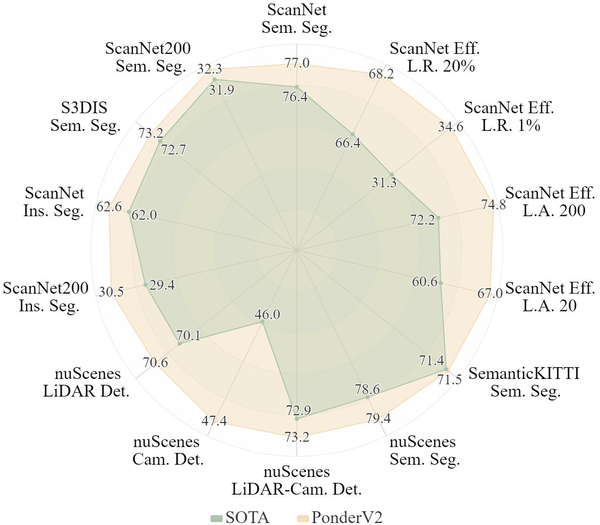
Figure 1: The radar chart of PonderV2, showing its effectiveness on over ten benchmarks in both indoor and outdoor scenarios. Abbreviations: sem. for semantic, ins. for instance, seg. for segmentation, eff. for efficient, L.R. for limited reconstructions, L.A. for limited annotations, obj. for object, rec. for reconstruction, cam. for camera, det. for detection. Note that the SOTA in the figure denotes the state-of-the-art performance with the same backbone as ours on validation sets.

Previous pre-training methods for obtaining effective 3D representation can be roughly categorized into two groups: contrast-based [25, 26, 27, 28, 29, 30, 31] and masked autoencoding-based (or completion-based) [32, 33, 34, 35, 36, 37, 38]. Contrast-based methods are designed to maintain invariant representation under different transformations. To achieve this, informative samples are required. In the 2D image domain, the above challenge is addressed by (1) introducing efficient positive/negative sampling methods, (2) using a large batch size and storing representative samples, and (3) applying various data augmentation policies. Inspired by these works, many works [25, 26, 27, 28, 29, 30, 31] are proposed to learn geometry-invariant features on 3D point cloud.

Methods using masked autoencoding are another line of research for 3D representation learning, which utilizes a pre-training task of reconstructing the masked point cloud based on partial observations. By maintaining a high masking ratio, such a simple task encourages the model to learn a holistic understanding of the input beyond low-level statistics. Although the masked autoencoders have been successfully applied in 2D images [12] and videos [39, 40], it remains challenging and still in exploration due to the inherent irregularity and sparsity of the point cloud data.

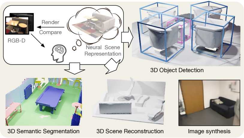
Figure 2: The proposed unified 3D pre-training approach, termed PonderV2, is directly trained with RGB-D rendered image supervision, and can be used for various indoor or outdoor 3D downstream applications, e.g., 3D object detection, 3D semantic segmentation, 3D scene reconstruction, and image synthesis, etc.

Different from the two groups of methods above, we propose point cloud pre-training via neural rendering (PonderV2), an extension of our preliminary work published at conference ICCV 2023 [41], as shown in Fig. 2. Our motivation is that neural rendering, one of the most amazing progress and domain-specific designs in 3D vision, can be leveraged to enforce the point cloud features being able to encode rich geometry and appearance cues. Why should rendering be considered the optimal choice for 3D representation learning? Drawing inspiration from the human visual system’s ability to intelligently perceive the 3D world through engagement with a 2D canvas, we realize that understanding and cognition inherently manifest in the 2D ‘rendering’ of the original 3D environment. Based on this fundamental principle, the conception of a rendering task as the foundation for 3D pre-training arises as the most intuitive bridge connecting the physical 3D world and the perceptual 2D realm. Specifically, 3D points are forwarded to a 3D encoder to learn the geometry and appearance of the scene via a neural representation, which is leveraged to render the RGB or depth images in a differentiable way. The network is trained to minimize the difference between rendered and observed 2D images. In doing so, our method implicitly encodes 3D space, facilitating the reconstruction of continuous 3D shape structures and the intricate appearance characteristics of their 2D projections. The flexibility of our method enables seamless integration into the 2D framework that takes as input multi-view images. Furthermore, given the 2D nature of the loss terms, it affords the flexibility to employ diverse signals for supervision, including RGB images, depth images, and annotated semantic labels.

Our methodology, though elegantly simple and readily implementable, stands as a testament to its robust performance. To validate its prowess, we conducted a battery of extensive experiments across a staggering array of over 9 indoor and outdoor tasks, including both high-level tasks such as indoor/outdoor segmentation and detection, as well as low-level tasks such as image synthesis and indoor scene/object reconstruction, etc. We achieve state-of-the-art performance on over 11 indoor/outdoor benchmarks. Part of PonderV2’s validation set performance compared to baselines and state-of-the-art methods with same backbone are shown in Fig. 1. The sufficient and convincing results indicate the effectiveness of the proposed universal methodology. Specifically, we first evaluate PonderV2 on different backbones on various popular indoor benchmarks with multi-frame RGB-D images as inputs, proving its flexibility. Furthermore, we pre-train a single backbone for various downstream tasks, namely SparseUNet [42], which takes whole-scene point clouds as input, and remarkably surpasses the state-of-the-art method with the same backbone on various indoor 3D benchmarks. For example, PonderV2 reaches $77.0$ val mIoU on ScanNet semantic segmentation benchmark and ranks $1$st on ScanNet benchmark with a test mIoU of $78.5$. PonderV2 also ranks $1$st on ScanNet200 semantic segmentation benchmark with a test mIoU of $34.6$. Finally, we conduct abundant experiments in outdoor autonomous driving scenarios, reaching SOTA validation performance as well. For example, we achieved 73.2 NDS for 3D detection and 79.4 mIoU for 3D segmentation on the nuScenes validation set, 3.0 and 6.1 higher than the baseline, respectively. The promising results display the efficacy of PonderV2.

To summarize, our contributions are listed below.

• We propose to utilize differentiable neural rendering as a novel universal pre-training paradigm tailored for the 3D vision realm. This paradigm, named PonderV2, captures the natural relationship between the 3D physical world and the 2D perception canvas.

• Our approach excels in acquiring efficient 3D representations, capable of encoding intricate geometric and visual cues through the utilization of neural rendering. This versatile framework extends its applicability to a range of modalities, encompassing both 3D and 2D domains, including but not limited to point clouds and multi-view images.

• The proposed methodology reaches state-of-the-art performance on many popular benchmarks of both indoor and outdoor, and is flexible to integrate into various backbones. Besides high-level perception tasks, PonderV2 can also boost low-level tasks such as image synthesis, scene and object reconstruction, etc. The effectiveness and flexibility of PonderV2 showcase the potential to pave the way for a 3D foundation model.

2 Related Works

Self-supervised learning in point clouds. Current methods can be roughly categorized into two categories: contrast-based and Masked Autoencoding-based. Inspired by the works [43, 44] from the 2D image domain, PointContrast [25] is one of the pioneering works for 3D contrastive learning. Similarly, it encourages the network to learn invariant 3D representation under different transformations. Some works [26, 27, 28, 29, 30, 31, 45] follow the pipeline by either devising new sampling strategies to select informative positive/negative training pairs, or explore various types of data augmentations. Another line of work is Masked Autoencoding-based [33, 34, 35, 36, 37, 38] methods, which get inspiration from Masked Autoencoders [12] (MAE). PointMAE [35] proposes restoring the masked points via a set-to-set Chamfer Distance. PointM2AE [37] utilizes a multiscale strategy to capture both high-level semantic and fine-grained details. VoxelMAE [38] instead recovers the underlying geometry by distinguishing if the voxel contains points. GD-MAE [46] applies a generative decoder for hierarchical MAE-style pre-training. Besides the above, ALSO [47] regards surface reconstruction as the pretext task for representation learning. Different from the above pipelines, we propose a novel framework for point cloud pre-training via neural rendering. Unlike previous works primarily designed for point clouds, our pre-training framework is applicable to both image- and point-based models.

Representation learning on images. Representation learning has been well-developed in the 2D domain [12, 48, 49, 43, 50, 40], and has shown its capabilities in all kinds of downstream tasks as the backbone initialization. Contrastive-based methods, such as MoCo [43] and MoCov2 [50], learn images’ representations by discriminating the similarities between different augmented samples. MAE-based methods, including MCMAE [51] and SparK [52], obtain the promising generalization ability by recovering the masked patches. Within the realm of 3D applications, models pre-trained on ImageNet [53] are widely utilized in image-related tasks [54, 55, 56, 57, 58, 59]. For example, to compensate for the insufficiency of 3D priors in tasks like 3D object detection, depth estimation [60] and monocular 3D detection [61] are usually used as extra pre-training techniques.

Neural rendering. Neural Rendering is a type of rendering technology that uses neural networks to render images from 3D scene representation in a differentiable way. NeRF [62] is one of the representative neural rendering methods, which represents the scene as the neural radiance field and renders the images via volume rendering. Based on NeRF, there are a series of works [63, 64, 65, 66, 67, 68, 69, 70, 71, 72, 41] trying to improve the NeRF representation, including accelerate NeRF training, boost the quality of geometry, and so on. Another type of neural rendering leverages neural point clouds as the scene representation. [73, 74] take points locations and corresponding descriptors as input, rasterize the points with z-buffer, and use a rendering network to get the final image. Later work such as PointNeRF [75] and X-NeRF [76] render realistic images from neural point representation using a NeRF-like rendering process. Our work is inspired by the recent progress of neural rendering.

3 Neural Rendering as a Universal Pre-training Paradiagm

In this section, we present the details of our methodology. We first give an overview of our pipeline in Sec. 3.1, which is visualized in Fig. 3. Then, we detail some specific differences and trials for indoor and outdoor scenarios due to the different input data types and settings in Sec. 3.2 and Sec. 3.3.

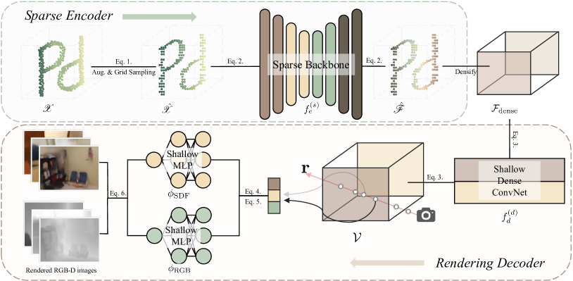
Figure 3: The overall piepeline of PonderV2. Taking a raw point cloud that can be constructed from multi-frame RGB-D images, scene scans and LiDAR, etc., we first apply augmentations including masking and grid sampling to obtain a quantized sparse tensor. Then, a sparse backbone is utilized to extract the sparse features and serves as the encoder to be pre-trained and finetuned in the future. After that, the sparse feature is densified and fed into a shallow dense convolutional networks, which gives out a dense feature volume. Next, the rendering decoder query features from the volume and applies shallow MLPs to output each point’s SDF and color value. Finally, the SDF and color outputs are integrated to render 2D RGB-D images which be will supervised by ground-truth.

3.1 Universal Pipeline Overview

As shown in Fig. 3, the input of our pipeline is an original sparse point cloud ${\mathscr{X}}=\{{\mathcal{C}}_{\mathrm{in}},{\mathcal{F}}_{\mathrm{in}}\}$ comprising a set of $n$ coordinates ${\mathcal{C}}_{\mathrm{in}}\in\mathbb{R}^{n\times 3}$ and their corresponding $ch_{in}$ channel features ${\mathcal{F}}_{\mathrm{in}}\in\mathbb{R}^{n\times ch_{in}}$ which may include attributes such as colors or intensities. These point clouds can be generated from a variety of sources, including RGB-D images, scans, or LiDAR data. Before diving into our backbone, we first apply augmentations to the input data and quantize it using a specific grid size ${\bm{g}}=[{g}_{x},{g}_{y},{g}_{z}]\in\mathbb{R}^{3}$. This process can be expressed as:

$$\hat{{\mathscr{X}}}={\mathbb{\mathcal{G}}}({\mathbb{\mathcal{T}}}({\mathscr{X}}),{\bm{g}}))=\{\hat{{\mathcal{C}}}_{\mathrm{in}},\hat{{\mathcal{F}}}_{\mathrm{in}}\}\text{,}$$ (1)

where ${\mathbb{\mathcal{G}}}(\cdot,{\bm{g}})$ is a grid sampling function designed to ensure that each grid has only one point sampled. ${\mathbb{\mathcal{T}}}(\cdot)$ denotes the augmentation transform function, and $\hat{{\mathscr{X}}}$ is the sampled points.

Then, we feed $\hat{{\mathscr{X}}}$ into a sparse backbone $f_{e}^{(s)}(\cdot)$, which serves as our pre-training encoder. The outputs are obtained by:

$$\hat{{\mathscr{F}}}=f_{e}^{(s)}(\hat{{\mathscr{X}}})=\{\hat{{\mathcal{C}}}_{\mathrm{out}},\hat{{\mathcal{F}}}_{\mathrm{out}}\},$$ (2)

where $\hat{{\mathcal{C}}}_{\mathrm{out}}$ and $\hat{{\mathcal{F}}}_{\mathrm{out}}$ are the coordinates and features of the sparse outputs, respectively. To make the sparse features compatible with our volume-based decoder, we encode them into a volumetric representation by a densification process. Specifically, we first discretize the 3D space at a resolution of $l_{x}\times l_{y}\times l_{z}$ voxel grids. Subsequently, the sparse features that fall into the same voxel are aggregated by applying average pooling based on their corresponding sparse coordinates. The aggregation will result in the dense volume features ${\mathcal{F}}_{\mathrm{dense}}\in\mathbb{R}^{l_{x}\times l_{y}\times l_{z}\times ch_{out}}$, where empty voxel grids are padded with zeros. A shallow dense convolutional network $f_{d}^{(d)}(\cdot)$ is then applied to obtain the enhanced 3D feature volume ${\mathcal{V}}\in\mathbb{R}^{l_{x}\times l_{y}\times l_{z}\times ch_{vol}}$, which can be expressed as:

$${\mathcal{V}}=f_{d}^{(d)}({\mathcal{F}}_{\mathrm{dense}})$$ (3)

Given the dense 3D volume ${\mathcal{V}}$, we make a novel use of differentiable volume rendering to reconstruct the projected color images and depth images as the pretext task. Inspired by [65], we represent a scene as an implicit signed distance function (SDF) field to be capable of representing high-quality geometry details. Specifically, given a camera pose ${\mathbf{P}}$ and sampled pixels ${\mathbf{x}}$, we shoot rays ${\mathbf{r}}$ from the camera’s projection center ${\mathbf{o}}$ in direction ${\mathbf{d}}$ towards the pixels, which can be derived from its intrinsics and extrinsics. Along each ray, we sample $D$ points $\{{\mathbf{p}}_{j}={\mathbf{o}}+t_{j}\cdot{\mathbf{d}}\mid j=1,...,D\land 0\leq t_{j}<t_{j+1}\}$, where $t_{j}$ is the distance from each point to camera center, and query each point’s 3D feature ${\mathbf{f}}_{j}$ from ${\mathcal{V}}$ by trilinear interpolation. A SDF value $s_{j}$ is predicted for each point ${\mathbf{p}}_{j}$ using an shallow MLP $\phi_{\mathrm{SDF}}$:

$$s_{j}=\phi_{\mathrm{SDF}}({\mathbf{p}}_{j},{\mathbf{f}}_{j})\text{,}$$ (4)

To determine the color value, our approach draws inspiration from [66] and conditions the color field on the surface normal ${\mathbf{n}}_{j}$ (i.e., the gradient of the SDF value at ray point ${\mathbf{p}}_{j}$) together with a geometry feature vector ${\mathbf{h}}_{i}$ derived from $\phi_{\mathrm{SDF}}$. This can yield a color representation:

$$c_{j}=\phi_{\mathrm{RGB}}({\mathbf{p}}_{j},{\mathbf{f}}_{j},{\mathbf{d}}_{i},{\mathbf{n}}_{j},{\mathbf{h}}_{j})\text{,}$$ (5)

where $\phi_{\mathrm{RGB}}$ is parameterized by another shallow MLP. Subsequently, we render 2D colors $\hat{C}({\mathbf{r}})$ and depths $\hat{D}({\mathbf{r}})$ by integrating predicted colors and sampled depths along rays ${\mathbf{r}}$ using the following equations:

$$\hat{C}({\mathbf{r}})=\sum_{j=1}^{D}{w_{j}c_{j}},\quad\hat{D}({\mathbf{r}})=\sum_{j=1}^{D}{w_{j}t_{j}},$$ (6)

The weight $w_{j}$ in these equations is an unbiased, occlusion-aware factor, as illustrated in [65], and is computed as $w_{j}=T_{j}\alpha_{j}$. Here, $T_{j}=\prod_{k=1}^{j-1}(1-\alpha_{k})$ represents the accumulated transmittance, while $\alpha_{j}$ is the opacity value computed by:

$$\alpha_{j}=\max\mathopen{}\mathclose{{}\left(\frac{\sigma_{s}\mathopen{}\mathclose{{}\left(s_{j}}\right)-\sigma_{s}\mathopen{}\mathclose{{}\left(s_{j+1}}\right)}{\sigma_{s}\mathopen{}\mathclose{{}\left(s_{j}}\right)},0}\right),$$ (7)

where $\sigma_{s}(x)=(1+e^{-sx})^{-1}$ is the $\operatorname{Sigmoid}$ function modulated by a learnable parameter $s$.

Finally, our optimization target is to minimize the $L^{1}$ reconstruction loss on rendered 2D pixel space with a $\lambda_{C}$ and a $\lambda_{D}$ factor adjusting the weight between color and depth, namely:

$$\mathcal{L}=\frac{1}{|{\mathbf{r}}|}\sum_{{\textnormal{r}}\in{\mathbf{r}}}\lambda_{C}\cdot\|\hat{C}({\textnormal{r}})-C({\textnormal{r}})\|+\lambda_{D}\cdot\|\hat{D}({\textnormal{r}})-D({\textnormal{r}})\|$$ (8)

3.2 Indoor Scenario

While the proposed rendering-based pretext task operates in a fully unsupervised manner, the framework can be easily extended to supervised learning by incorporating off-the-shelf labels to further improve the learned representation. Due to the large amount of synthetic data with available annotations for indoor scenes, the rendering decoder could additionally render semantic labels in 2D. Specifically, we employ an additional shallow MLP, denoted as $\phi_{\mathrm{SEMANTIC}}$, to predict semantic features for each query point:

$${\mathbf{l}}_{j}=\phi_{\mathrm{SEMANTIC}}({\mathbf{p}}_{j},{\mathbf{f}}_{j},{\mathbf{n}}_{j},{\mathbf{h}}_{j})\text{,}$$ (9)

These semantic features can be projected onto a 2D canvas using a similar weighting scheme as described in Eq. 6. For supervision, we utilize the CLIP [13] features of each pixel’s text label which is a readily available attribute in most indoor datasets.

It is worth noting that when handling vast amounts of unlabeled RGB-D data, the semantic rendering can also be switched to an unsupervised manner by leveraging existing 2D segmentation models. For example, alternative approaches such as utilizing Segment-Anything [8], or diffusion [77] features to provide pseudo semantic features as supervision, which can also distill knowledge from 2D foundational models into 3D backbones. Further research on this aspect is left as future work, as the primary focus of this paper is the novel pre-training methodology itself.

3.3 Outdoor Scenario

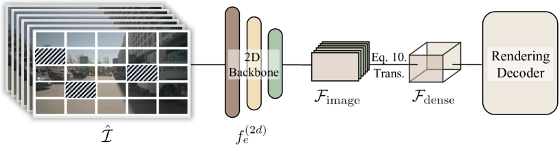
Figure 4: The overall piepeline of multi-image input. The rendering decoder is the same as Fig. 3. The image encoder takes augmented multi-view images as inputs, giving out the multi-view features. The image features are then zero-padded and transformed to obtain the 3D dense feature volume.

To further show the generalization ability of our pre-training paradigm, we also have applied our methodology to the outdoor scenario, where multi-view images and LiDAR point clouds are usually available. To make the pre-training method suitable for these inputs, we convert them into the 3D volumetric space.

Specifically, for the LiDAR point clouds, we follow the same process in Sec. 3.1 to augment the point clouds and voxelize the point features extracted by a 3D backbone.

For multi-view images ${\mathcal{I}}=\{{\bm{I}}_{1},{\bm{I}}_{2},...\}$, inspired by MAE [12], we first mask out partial pixels as the data augmentation to get $\hat{{\mathcal{I}}}$. Then we leverage a 2D backbone $f_{e}^{(2d)}$ to extract multi-view image features ${\mathcal{F}}_{\mathrm{image}}=f_{e}^{(2d)}(\hat{{\mathcal{I}}})$. The 2D features are subsequently transformed into the 3D ego-car coordinate system to obtain the 3D dense volume features. Concretely, we first pre-define the 3D voxel coordinates $X_{p}\in\mathbb{N}^{l_{x}\times l_{y}\times l_{z}\times 3}$, and then project $X_{p}$ on multi-view images to index the corresponding 2D features. The process can be calculated by:

$${\mathcal{F}}_{\mathrm{dense}}={\mathcal{B}}(T_{\mathrm{c2i}}T_{\mathrm{l2c}}X_{p},{\mathcal{F}}_{\mathrm{image}}),$$ (10)

where $T_{\mathrm{l2c}}$ and $T_{\mathrm{c2i}}$ denote the transformation matrices from the LiDAR coordinate system to the camera frame and from the camera frame to image coordinates, respectively, and ${\mathcal{B}}$ represents the bilinear interpolation. The encoding process of the multi-view image case is shown in Fig. 4.

4 Experiments for Indoor Scenarios

We first conduct comprehensive experiments on indoor datasets, which mainly contain two parts. In the first part, we use a lightweight backbone for ablation studies, which take as input multi-frame RGB-D only. We call this variant Ponder-RGBD. The subsequent part mainly focuses on a single, unified pre-trained model that pushes to the limits of performance, surpassing the previous SOTA pretraining pipeline substantially.

4.1 Indoor Multi-frame RGB-Ds as Inputs

4.1.1 Experimental Setup

We use ScanNet [78] RGB-D images as our pre-training dataset. ScanNet is a widely used real-world indoor dataset, which contains more than 1500 indoor scenes. Each scene is carefully scanned by an RGB-D camera, leading to about 2.5 million RGB-D frames in total. We follow the same train / val split with VoteNet [79]. In this part, we have not introduced semantic rendering yet, which will be used in the part of scene-level as inputs.

4.1.2 Implementation and Training Details

For the version of RGB-D inputs, $3$ input channels of RGB is taken with grid size ${\bm{g}}=0.02^{3}$. After densifying ${\mathcal{V}}$ to $64\times 64\times 64$ with $96$ channels, we apply a dense UNet with an output channel number of $128$. $\phi_{\mathrm{SDF}}$ is designed as a $5$-layer MLP while $\phi_{\mathrm{RGB}}$ is a $3$-layer MLP.

During pre-training, a mini-batch of batch size $8$ includes point clouds from $8$ scenes. Each point cloud input to our sparse backbone is back-projected from $5$ continuous RGB-D frames of a video from ScanNet’s raw data with a frame interval of $20$. The $5$ frames are also used as the supervision of the network. We randomly down-sample the input point cloud to 20,000 points and follow the masking strategy as used in Mask Point [36].

We train the proposed pipeline for 100 epochs using an AdamW optimizer [80] with a weight decay of $0.05$. The learning rate is initialized as $1e^{-4}$ with an exponential schedule. For the rendering process, we randomly choose 128 rays for each image and sample 128 points for each ray.

4.1.3 Comparison Experiments

TABLE I: Indoor Ponder-RGBD 3D object detection mAP@25 and mAP@50 on ScanNet and SUN RGB-D with VoteNet [79] backbone. The DepthContrast [31] and Point-BERT [33] results are adopted from IAE [34] and MaskPoint [36]. Ponder-RGBD outperforms both VoteNet-based and 3DETR-based point cloud pre-training methods with fewer training epochs.

Method	Detection Model	Pre-training Type	Pre-training Epochs	ScanNet Val		SUN RGB-D Val
				mAP@50	mAP@25	mAP@50	mAP@25
3DETR [81]	3DETR	-	-	37.5	62.7	30.3	58
+ Point-BERT [33]	3DETR	Masked Auto-Encoding	300	38.3	61.0	-	-
+ MaskPoint [36]	3DETR	Masked Auto-Encoding	300	40.6	63.4	-	-
VoteNet [79]	VoteNet	-	-	33.5	58.6	32.9	57.7
+ STRL [28]	VoteNet	Contrast	100	38.4	59.5	35.0	58.2
+ RandomRooms [30]	VoteNet	Contrast	300	36.2	61.3	35.4	59.2
+ PointContrast [25]	VoteNet	Contrast	-	38.0	59.2	34.8	57.5
+ PC-FractalDB [82]	VoteNet	Contrast	-	38.3	61.9	33.9	59.4
+ DepthContrast [31]	VoteNet	Contrast	1000	39.1	62.1	35.4	60.4
+ IAE [34]	VoteNet	Masked Auto-Encoding	1000	39.8	61.5	36.0	60.4
+ Ponder-RGBD (Ours)	VoteNet	Rendering	100	41.0↑7.5	63.6↑5.0	36.6↑3.7	61.0↑3.3

TABLE II: Indoor Ponder-RGBD 3D object detection mAP@25 and mAP@50 on ScanNet validation set with H3DNet [83] backbone. Ponder-RGBD significantly boosts the accuracy by a margin of +2.8 and +1.2 for mAP@50 and mAP@25, respectively.

Method	mAP@50	mAP@25
VoteNet [79]	33.5	58.7
3DETR [81]	37.5	62.7
3DETR-m [81]	47.0	65.0
H3DNet [83]	48.1	67.2
+ Ponder-RGBD (Ours)	50.9↑2.8	68.4↑1.2

Object Detection We select two representative approaches, Votenet [79] and H3DNet [83], as the baselines. VoteNet leverages a voting mechanism to obtain object centers, which are used for generating 3D bounding box proposals. By introducing a set of geometric primitives, H3DNet achieves a significant improvement in accuracy compared to previous methods. Two datasets are applied to verify the effectiveness of our method: ScanNet [78] and SUN RGB-D [84]. Different from ScanNet, which contains fully reconstructed 3D scenes, SUN RGB-D is a single-view RGB-D dataset with 3D bounding box annotations. It has 10,335 RGB-D images for 37 object categories. For pre-training, we use PointNet++ as the point cloud encoder $f_{e}^{(s)}$, which is identical to the backbone used in VoteNet and H3DNet. We pre-train $f_{e}^{(s)}$ on the ScanNet dataset and transfer the weight as the downstream initialization. Following [79], we use average precision with 3D detection IoU threshold $0.25$ and threshold $0.5$ as the evaluation metrics.

The 3D detection results are shown in Tab. I. Our method improves the baseline of VoteNet without pre-training by a large margin, boosting mAP@50 by 7.5% and 3.7% for ScanNet and SUN RGB-D, respectively. IAE [34] is a pre-training method that represents the inherent 3D geometry in a continuous manner. Our learned point cloud representation achieves higher accuracy because it is able to recover both the geometry and appearance of the scene. The mAP@50 and mAP@25 of our method are higher than that of IAE by 1.2% and 2.1% on ScanNet, respectively. Besides, we have observed that our method surpasses the recent point cloud pre-training approach, MaskPoint [36], even when using a less sophisticated backbone (PointNet++ vs. 3DETR), as presented in Tab. I. To verify the effectiveness of Ponder-RGBD, we also apply it for a much stronger baseline, H3DNet. As shown in Tab. II, our method surpasses H3DNet by +2.8 and +1.2 for mAP@50 and mAP@25, respectively.

Semantic Segmentation 3D semantic segmentation is another fundamental scene understanding task. We select one of the top-performing backbones, MinkUNet [42], for finetuning. MinkUNet leverages 3D sparse convolution to extract effective 3D scene features. We report the finetuning results on the ScanNet dataset with the mean IoU of the validation set as the evaluation metric. Tab. III shows the quantitative results of Ponder-RGBD with MinkUNet. The results demonstrate that Ponder-RGBD is effective in improving the semantic segmentation performance, achieving a significant improvement of 1.3 mIoU.

Scene Reconstruction 3D scene reconstruction task aims to recover the scene geometry, e.g. mesh, from the point cloud input. We choose ConvONet [85] as the baseline model, whose architecture is widely adopted in [86, 87, 64]. Following the same setting as ConvONet, we conduct experiments on the Synthetic Indoor Scene Dataset (SISD) [85], which is a synthetic dataset and contains 5000 scenes with multiple ShapeNet [88] objects. To make a fair comparison with IAE [34], we use the same VoteNet-style PointNet++ as the encoder of ConvONet, which down-samples the original point cloud to 1024 points. Following [85], we use Volumetric IoU, Normal Consistency (NC), and F-Score [89] with the threshold value of 1% as the evaluation metrics. The results are shown in Tab. IV. Compared to the baseline ConvONet model with PointNet++, IAE is not able to boost the reconstruction results, while the proposed approach can improve the reconstruction quality (+2.4% for IoU). The results show the effectiveness of Ponder-RGBD for the 3D scene reconstruction task.

TABLE III: Indoor Ponder-RGBD 3D segmentation mIoU on ScanNet validation dataset.

Method	Val mIoU
PointNet++ [90]	53.5
KPConv [91]	69.2
SparseConvNet [92]	69.3
PT [93]	70.6
MinkUNet [42]	72.2
+ Ponder-RGBD (Ours)	73.5↑1.3

TABLE IV: Indoor Ponder-RGBD 3D scene reconstruction IoU, NC, and F-Score on SISD dataset with PointNet++ backbone. Ponder-RGBD can boost the scene reconstruction performance.

Method	Encoder	IoU$\uparrow$	NC$\uparrow$	F-Score$\uparrow$
IAE [34]	PointNet++	75.7	88.7	91.0
ConvONet [85]	PointNet++	77.8	88.7	90.6
+ Ponder-RGBD (Ours)	PointNet++	80.2↑2.4	89.3↑0.6	92.0↑1.4

Image Synthesis From Point Clouds We also validate the effectiveness of our method on another low-level task of image synthesis from point clouds. We use Point-NeRF [75] as the baseline. Point-NeRF uses neural 3D point clouds with associated neural features to render images. It can be used both for a generalizable setting for various scenes and a single-scene fitting setting. In our experiments, we mainly focus on the generalizable setting of Point-NeRF. We replace the 2D image features of Point-NeRF with point features extracted by a DGCNN network. Following the same setting with PointNeRF, we use DTU [94] as the evaluation dataset. DTU dataset is a multiple-view stereo dataset containing 80 scenes with paired images and camera poses. We transfer both the DGCNN encoder and color decoder as the weight initialization of Point-NeRF. We use PSNR as the metric for synthesized image quality evaluation.

The results are shown in Fig. 6. By leveraging the pre-trained weights of our method, the image synthesis model is able to converge faster with fewer training steps and achieve better final image quality than training from scratch.

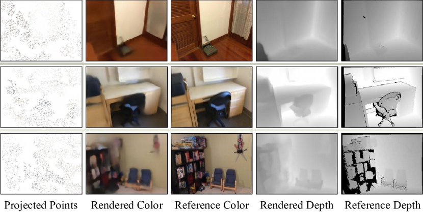
Figure 5: Rendered images by Ponder-RGBD on the ScanNet validation set. The projected point clouds are visualized in the first column. Even though input point clouds are very sparse, our model is capable of rendering color and depth images similar to the reference images.

Ponder-RGBD’s rendered color images and depth images are shown in Fig. 5. As shown in the figure, even though the input point cloud is pretty sparse, our method is still capable of rendering color and depth images similar to the reference image.

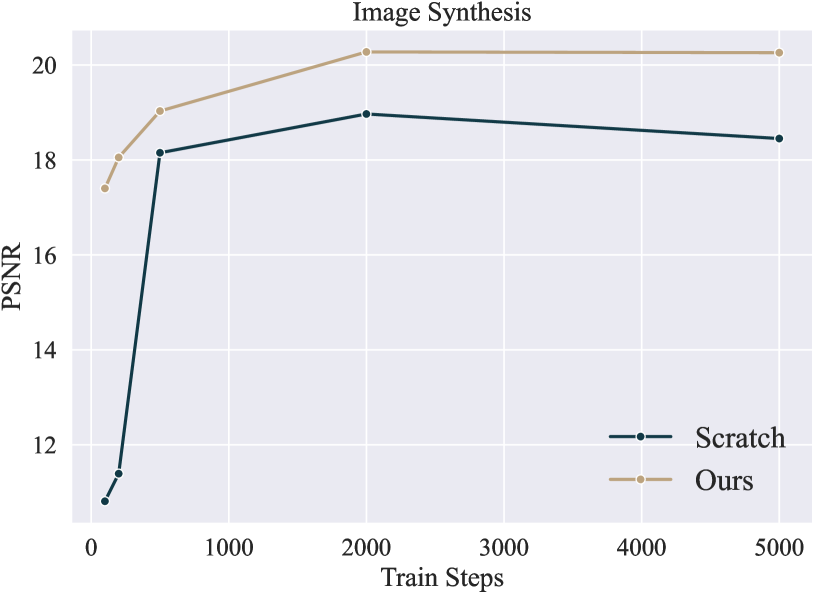
Figure 6: Comparison of image synthesis from point clouds. Compared with training from scratch, our Ponder-RGBD model is able to converge faster and achieve better image synthesis results.

4.1.4 Ablation Study

Influence of Rendering Targets The rendering part of our method contains two items: RGB color image and depth image. We study the influence of each item with the transferring task of 3D detection. The results are presented in Tab. V. Combining depth and color images for reconstruction shows the best detection results. In addition, using depth reconstruction presents better performance than color reconstruction for 3D detection.

Influence of Mask Ratio To augment point cloud data, we employ random masking as one of the augmentation methods, which divides the input point cloud into 2048 groups with 64 points. In this ablation study, we evaluate the performance of our method with different mask ratios, ranging from 0% to 90%, on the ScanNet and SUN RGB-D datasets, and report the results in Tab. VI. Notably, we find that even when no dividing and masking strategy is applied (0%), our method achieves a competitive mAP@50 performance of 40.7 and 37.3 on ScanNet and SUN RGB-D, respectively. Our method achieves the best performance on ScanNet with a mask ratio of 75% and a mAP@50 performance of 41.7. Overall, these results suggest that our method is robust to the hyper-parameter of mask ratio and can still achieve competitive performance without any mask operation.

Influence of 3D Feature Volume Resolution In our method, Ponder-RGBD constructs a 3D feature volume with a resolution of [16, 32, 64], which is inspired by recent progress in multi-resolution 3D reconstruction. However, building such a high-resolution feature volume can consume significant GPU memory. To investigate the effect of feature volume resolution, we conduct experiments with different resolutions and report the results in Tab. VII. From the results, we observe that even with a smaller feature volume resolution of 16, Ponder-RGBD can still achieve competitive performance on downstream tasks.

TABLE V: Indoor Ponder-RGBD ablation study for supervision type. 3D detection $\textit{{AP}}_{50}$ on ScanNet and SUN RGB-D validation set. Combining color supervision and depth supervision can lead to better detection performance than using a single type of supervision.

Supervision	ScanNet mAP@50	SUN RGB-D mAP@50
VoteNet	33.5	32.9
+ Depth	40.9↑7.4	36.1↑3.2
+ Color	40.5↑7.0	35.8↑2.9
+ Depth + Color	41.0↑7.5	36.6↑3.7

TABLE VI: Ablation study for mask ratio. 3D detection $\textit{{AP}}_{50}$ on ScanNet and SUN RGB-D validation set.

Mask Ratio	ScanNet mAP@50	SUN RGB-D mAP@50
VoteNet	33.5	32.9
0%	40.7↑7.2	37.3↑4.4
25%	40.7↑7.2	36.2↑3.3
50%	40.3↑6.8	36.9↑4.0
75%	41.7↑8.2	37.0↑4.1
90%	41.0↑7.5	36.6↑3.7

TABLE VII: Ablation study for feature volume resolution. 3D detection $\textit{{AP}}_{50}$ on ScanNet and SUN RGB-D validation set.

Resolution	ScanNet mAP@50	SUN RGB-D mAP@50
VoteNet	33.5	32.9
16	40.7↑7.2	36.6↑3.7
16 + 32 + 64	41.0↑7.5	36.6↑3.7

TABLE VIII: Ablation study for view number. 3D detection $\textit{{AP}}_{50}$ on ScanNet and SUN RGB-D validation set. Using multi-view supervision for pre-training can achieve better performance.

#View	ScanNet mAP@50	SUN RGB-D mAP@50
VoteNet	33.5	32.9
1	40.1↑6.6	35.4↑2.5
3	40.8↑7.3	36.0↑3.1
5	41.0↑7.5	36.6↑3.7

Number of Input RGB-D View. Our method utilizes $N$ RGB-D images, where $N$ is the input view number. We study the influence of $N$ and conduct experiments on 3D detection, as shown in Tab. VIII. We change the number of input views while keeping the scene number of a batch still 8. Using multi-view supervision helps to reduce single-view ambiguity. Similar observations are also found in the multi-view reconstruction task [95]. Compared with the single view, multiple views achieve higher accuracy, boosting mAP@50 by 0.9% and 1.2% for ScanNet and SUN RGB-D datasets, respectively.

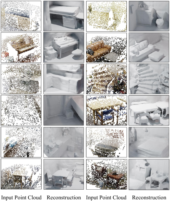
Figure 7: Reconstructed surface by Ponder-RGBD. Our pre-training method can be easily integrated into the task of 3D reconstruction. Despite the sparsity of the input point cloud (only 2% points are used), our method can still recover precise geometric details.

4.1.5 Other applications

The pre-trained model from our pipeline Ponder-RGBD itself can also be directly used for surface reconstruction from sparse point clouds. Specifically, after learning the neural scene representation, we query the SDF value in the 3D space and leverage the Marching Cubes [96] to extract the surface. We show the reconstruction results in Fig. 7. The results show that even though the input is sparse point clouds from complex scenes, our method is able to recover high-fidelity meshes.

4.2 Indoor Scene Point Clouds as Inputs

TABLE IX: Indoor semantic segmentation results. Our method builds on SparseUNet [42], and is evaluated on ScanNet [78], ScanNet200 [97], and S3DIS [98] benchmarks. Compared to other pre-training approaches, PonderV2 has significant finetuning improvements across all the benchmarks with shared pre-trained weights.

Method	#Params.	ScanNet		ScanNet200		S3DIS
		Val mIoU	Test mIoU	Val mIoU	Test mIoU	Area5 mIoU	6-fold mIoU
StratifiedFormer [99]	18.8M	74.3	73.7	-	-	72.0	78.1
PointNeXt [100]	41.6M	71.5	71.2	-	-	70.5	77.2
PTv1 [93]	11.4M	70.6	-	27.8	-	70.4	76.5
PTv2 [101]	12.8M	75.4	75.2	30.2	-	71.6	77.9
SparseUNet [42]	39.2M	72.2	73.6	25	25.3	65.4	65.4
+ PC [25]	39.2M	74.1	-	26.2	-	70.3	76.9
+ CSC [26]	39.2M	73.8	-	26.4	24.9	72.2	-
+ MSC [45]	39.2M	75.5	-	28.8	-	70.1	77.2
+ PPT [102]	41.0M	76.4	76.6	31.9	33.2	72.7	78.1
+ PonderV2 (Ours)	41.0M	77.0↑4.8	78.5↑4.9	32.3↑7.3	34.6↑9.3	73.2↑7.8	79.1↑13.7

TABLE X: Indoor S3DIS semantic segmentation 6-fold cross-validation results. PonderV2 achieves the best average performance on all metrics including mIoU, mAcc and allAcc.

Metric	Area1		Area2		Area3		Area4		Area5		Area6		Average
	PPT	PonderV2	PPT	PonderV2	PPT	PonderV2	PPT	PonderV2	PPT	PonderV2	PPT	PonderV2	PPT	PonderV2	Scratch
mIoU	83.0	84.1	65.4	72.3	87.1	886.1	74.1	73.4	72.7	73.2	86.4	87.4	78.1	79.9↑1.8	65.4
mAcc	90.3	90.8	75.6	78.6	91.8	91.6	84.0	81.9	78.2	79.0	92.5	92.8	85.4	86.5↑1.1	-
allAcc	93.5	93.7	88.3	91.6	94.6	94.2	90.8	90.8	91.5	92.2	94.5	94.8	92.2	92.5↑0.3	-

4.2.1 Experimental Setup

In this setting, we want to pre-train a unified backbone that can be applied to various downstream tasks, whose input is directly the whole scene point clouds so that the upstream and downstream models have a unified input and encoder stage. We choose SparseUNet [42], which is an optimized implementation of MinkUNet [42] by SpConv [103], as $f_{e}^{(s)}$ due to its efficiency, whose out features $\hat{{\mathscr{F}}}$ have $96$ channels. We mainly focus on three widely recognized indoor datasets: ScanNet [78], S3DIS [104] and Structured3D [105] to jointly pre-train our weights. ScanNet and S3DIS represent the most commonly used real-world datasets in the realm of 3D perception, while Structured3D is a synthetic RGB-D dataset. Given the limited data diversity available in indoor 3D vision, there exists a non-negligible domain gap between datasets, thus naive joint training may not boost performance. Point Prompt Training [102] (PPT) proposes to address this problem by giving each dataset its own batch norm layer. Considering its effectiveness and flexibility, we combine PPT with our universal pre-training paradigm and treat PPT as our baseline. Notably, PPT achieves state-of-the-art performance in downstream tasks with the same backbone we use, i.e., SparseUNet.

Following the pre-training phase, we discard the rendering decoder and load the encoder backbone’s weights for use in downstream tasks, either with or without additional task-specific heads. Subsequently, the network undergoes fine-tuning and evaluation on each specific downstream task. We mainly evaluate the mean intersection-over-union (mIoU) metric for semantic segmentation and mean average precision (mAP) for instance segmentation as well as object detection tasks.

4.2.2 Implementation and Training Details

For the version of the unified backbone, we base our indoor experiments on Pointcept [106], a powerful and flexible codebase for point cloud perception research. All hyper-parameters are the same with scratched PPT, for fair comparison. The number of input channels for this setting is $6$, containing $3$ channels of colors and $3$ channels of surface normals. Grid size ${\bm{g}}$ is same as $0.02^{3}$ meters. We also apply common transformations including random dropout (at a mask ratio of $0.8$), rotation, scaling, flipping, etc.

Considering that although a lightweight decoder reduces the rendering effect, it may boost downstream performance, we use a tiny dense 3D UNet with channels of $128$ after densifying. The dense feature volume ${\mathcal{V}}$ is configured to be of size $128\times 128\times 32$ with $128$ channels. $\phi_{\mathrm{SDF}}$ is a shallow MLP with $3$ layers and $\phi_{\mathrm{RGB}}$ as well as $\phi_{\mathrm{SEMANTIC}}$ are both $1$-layer MLPs. All shallow MLPs have a hidden channel of $128$. For semantic supervision, we use the text encoder of a ”ViT-B/16” CLIP model, whose output semantic features are of $512$ channels.

In each scene-level input point cloud, we first sample $5$ RGB-D frames for supervision, from which we subsequently sample $128$ rays each. Consequently, a total of $128\times 5=640$ pixel values per point cloud are supervised in each iteration. Notably, the weight coefficient $\lambda_{C}$ is $1.0$ and $\lambda_{D}$ is set to $0.1$.

We train the proposed pipeline for $200$ epochs using an SGD optimizer with a weight decay of $1e^{-4}$ and a momentum of $0.9$. The learning rate is initialized as $8e^{-4}$ with with a one-cycle scheduler [107]. For the rendering process, we randomly choose $5$ frames for each point cloud, $128$ rays for each image, and sample $128$ points for each ray. The batch size of point clouds is set to $64$. Models are trained on $8$ NVIDIA A100 GPU. More implementation details can be found in the supplementary materials.

4.2.3 Comparison Experiments

Semantic Segmentation We conduct indoor semantic segmentation experiments on ScanNet, S3DIS and Structured3D. We take PPT, the SOTA method using SparseUNet [42], as our baseline, and report the comparison performance of scratch and finetuned models in Tab. IX. The S3DIS dataset contains 6 areas, among which we usually take Area 5 as the validation set. It is also common to evaluate 6-fold performance on it, so we also report the detailed 6-fold results in Tab. X. Note that to avoid information leaks, we pre-train a new model on only ScanNet and Structured3D before finetuning on each area of the S3DIS dataset. The semantic segmentation experiments all show the significant performance of our proposed paradigm.

TABLE XI: Indoor instance segmentation results. With the same pre-trained weights, we further fine-tune PonderV2 on ScanNet and ScanNet200 instance segmentation driven by PointGroup [108]. We compare mAP@25, mAP@50, and mAP results with previous pre-training methods, and our method shows superior results across benchmarks.

Method	#Params.	Scannet			ScanNet200
		mAP@25	mAP@50	mAP	mAP@25	mAP@50	mAP
PointGroup [108]	39.2M	72.8	56.9	36.0	32.2	24.5	15.8
+ PC [25]	39.2M	-	58.0	-	-	24.9	-
+ CSC [26]	39.2M	-	59.4	-	-	25.2	-
+ LGround [97]	39.2M	-	-	-	-	26.1	-
+ MSC [45]	39.2M	74.7	59.6	39.3	34.3	26.8	17.3
+ PPT [102]	41.0M	76.9	62.0	40.7	36.8	29.4	19.4
+ PonderV2 (Ours)	41.0M	77.0↑4.2	62.6↑5.7	40.9↑4.9	37.6↑5.4	30.5↑6.0	20.1↑4.3

Instance Segmentation 3D instance segmentation is another fundamental perception task. We benchmark our finetuning results on ScanNet, ScanNet200 and S3DIS (Area 5), which is shown in Tab. XI. The results show that our pre-training approach also helps enhance instance segmentation understanding.

TABLE XII: Indoor data efficient results. We follow the ScanNet Data Efficient benchmark [26] and compare the validation results of PonderV2 with previous pre-training methods. All methods are trained with SparseUNet. Pct. in limited reconstructions setting denotes the percentage of scene reconstruction that could be used for training. #Pts. in limited annotations setting denotes the number of points per scene that are annotated for training.

Pct.	Limited Reconstructions					#Pts.	Limited Annotations
	Sratch	CSC [26]	MSC [45]	PPT	PonderV2		Sratch	CSC [26]	MSC [45]	PPT	PonderV2
1%	26.0	28.9	29.2	31.3	34.6↑8.6	20	41.9	55.5	60.1	60.6	67.0↑25.1
5%	47.8	49.8	59.4	52.2	56.5↑8.7	50	53.9	60.5	66.8	67.5	72.2↑18.3
10%	56.7	59.4	61.0	62.8	66.0↑9.3	100	62.2	65.9	69.7	70.8	74.3↑12.1
20%	62.9	64.6	64.9	66.4	68.2↑5.3	200	65.5	68.2	70.7	72.2	74.8↑9.3
100%	72.2	73.8	75.3	76.4	77.0↑4.8	Full	72.2	73.8	75.3	76.4	77.0↑4.8

Data Efficiency on ScanNet The ScanNet benchmark also contains data efficiency settings of limited annotations (LA) and limited reconstructions (LR). In the LA setting, the models are allowed to see only a small ratio of labels while in the LR setting, the models can only see a small number of reconstructions (scenes). Again, to prevent information leaking, we pre-train our model on only S3DIS and Structured3D before finetuning. Results in Tab. XII indicate that our approach is more data efficient compared to the baseline.

TABLE XIII: Object reconstruction results on CO3D dataset.

	F1-Score
MCC [109]	63.5
+ SparseUNet [42]	63.9
+ PonderV2	65.6↑2.1

Object Reconstruction Besides high-level perception tasks, we also conduct object reconstruction experiments to see if PonderV2 can work for low-level tasks. We take MCC [109] as our baseline and evaluate on a subset of CO3D [110] dataset for fast validation. CO3D is a 3D object dataset that can be used for object-level reconstruction. Specifically, we choose $1573$ train samples and $224$ test samples from $10$ categories including parkingmeter, baseball glove, toytrain, donut, skateboard, hotdog, frisbee, tv, sandwich and toybus. We train models for 100 epochs with a learning rate of $1e^{-4}$ and an effective batch size of $64$. The problem is evaluated by the predicted occupancy of a threshold of $0.1$, the same as in MCC’s original paper. The evaluation metric is F1-Score on the occupancies. For a fair comparison, we first directly change MCC’s encoder to our SparseUNet [42]. Then we average-pool the output volume into a 2D feature map and use MCC’s patch embedding module to align with the shape of the decoder’s input. Moreover, we adjust the shrink threshold from default $10.0$ to $3.0$, which increases the number of valid points after grid sampling. After this modification, the scratched baseline result is slightly higher than the original MCC’s, as shown in Tab. XIII. Moreover, we find that if finetuned with our pre-trained weights, it can remarkably gain nearly 2 points higher F1-Score. Note that the loaded weight is the same as previous high-level tasks, i.e. it is trained on scene-level ScanNet, Structured3D, and S3DIS datasets. We directly ignore the first layer as well as the final layer of weight before finetuning, since MCC does not take normal as input and requires a different number of output channels. The results indicate that not only can our approach work well on low-level tasks, but also that the proposed method has the potential to transfer scene-level knowledge to object-level.

5 Experiments for Outdoor Scenarios

As shown in Fig. 8, PonderV2 achieves significant improvements across various 3D outdoor tasks of different input modality, which further prove the universal effectiveness of proposed methodology. In this section, we detail the experimental details of PonderV2’s outdoor experiments as follows.

5.1 Experimental Setup

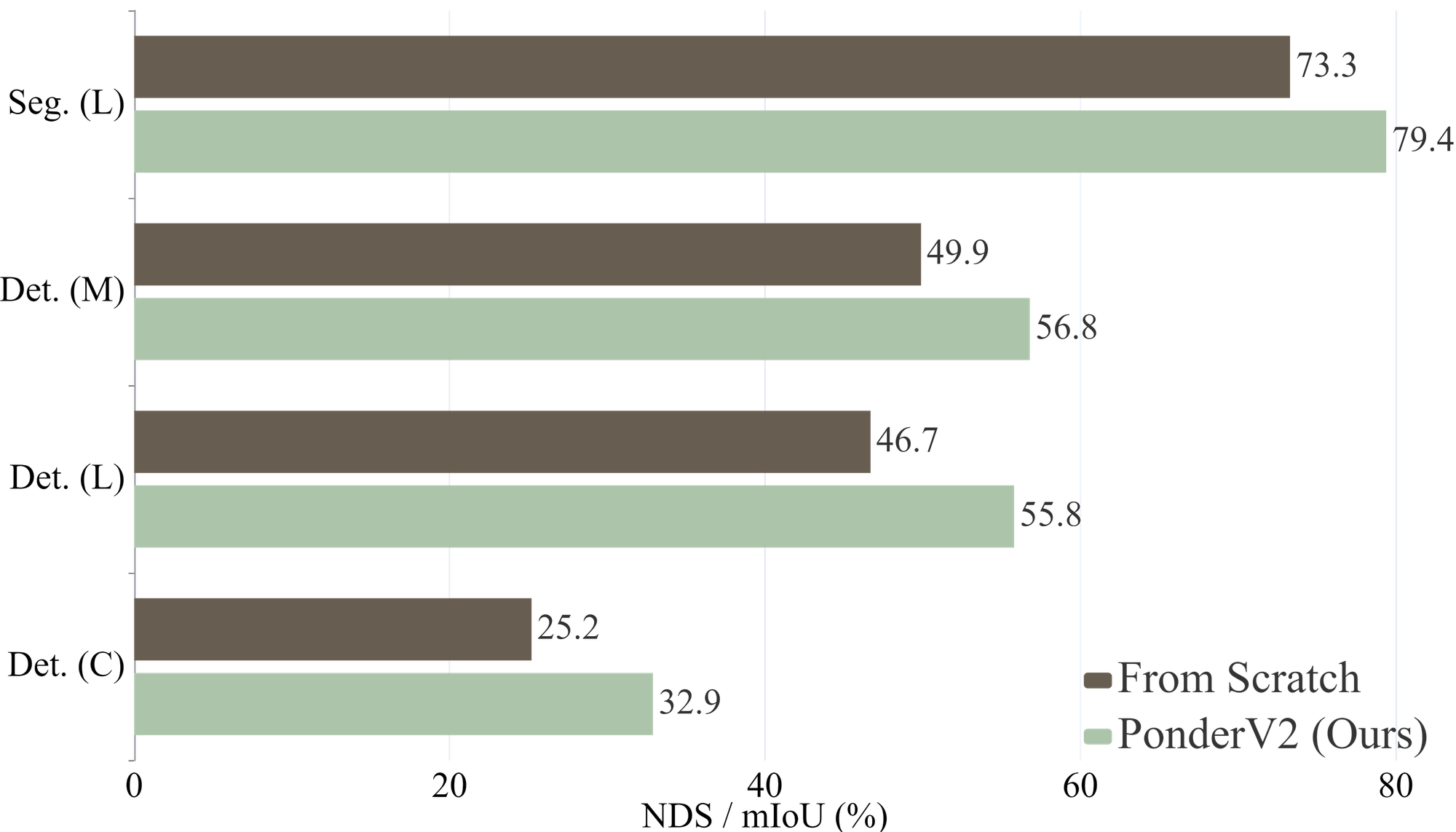
Figure 8: Effect of our pre-training for 3D outdoor detection and segmentation, where C, L, and M denote camera, LiDAR, and fusion modality, respectively.

We conduct the experiments on the NuScenes [111] dataset, which is a challenging dataset for autonomous driving. It consists of 700 scenes for training, 150 scenes for validation, and 150 scenes for testing. Each scene is captured through six different cameras, providing images with surrounding views, and is accompanied by a point cloud from LiDAR. The dataset comes with diverse annotations, supporting tasks like 3D object detection and 3D semantic segmentation. For detection evaluation, we employ nuScenes detection score (NDS) and mean average precision (mAP), and for segmentation assessment, we use mean intersection-over-union (mIoU).

5.2 Implementation and Training Details

We base our code on the MMDetection3D [112] toolkit and train all models on 4 NVIDIA A100 GPUs. The input image is configured to $1600\times 900$ pixels, while the voxel dimensions ${\bm{g}}$ for point cloud voxelization are $[0.075,0.075,0.2]$. During the pre-training phase, we implemented several data augmentation strategies, such as random scaling and rotation. Additionally, we partially mask the inputs, focusing only on visible regions for feature extraction. The masking size and ratio for images are configured to $32$ and $0.3$, and for points to $8$ and $0.8$, respectively. For the segmentation task, we use SparseUNet as our sparse backbone $f_{e}^{(e)}$, and for the detection task, we use VoxelNet [113], which is similar to the encoder part of SparseUNet, as our backbone. For multi-image setting, we use ConvNeXt-small [114] as our feature extractor $f_{e}^{(2d)}$. A uniform voxel representation ${\mathcal{V}}$ with the shape of $180\times 180\times 5$ is constructed. The $f_{d}^{(d)}$ here is a $3$-kernel size convolution which serves as a feature projection layer reducing the ${\mathcal{V}}$’s feature dimension to $32$. For the rendering decoders, we utilize a $6$-layer MLP for $\phi_{\mathrm{SDF}}$ and a $4$-layer MLP for $\phi_{\mathrm{RGB}}$. In the rendering phase, $512$ rays per image view and $96$ points per ray are randomly selected. We maintain the loss scale factors for $\lambda_{\mathrm{RGB}}$ and $\lambda_{\mathrm{depth}}$ at $10$. The model undergoes training for $12$ epochs using the AdamW optimizer with initial learning rates of $2e^{-5}$ and $1e^{-4}$ for point and image modalities, respectively. In the ablation studies, unless explicitly stated, fine-tuning is conducted for $12$ epochs on 50% of the image data and for $20$ epochs on 20% of the point data, without the implementation of the CBGS [115] strategy.

5.3 Outdoor Comparison Experiments

3D Object Detection In Table XIV, we compare PonderV2 with previous detection approaches on the nuScenes validation set. We adopt UVTR [57] as our baselines for point-modality (UVTR-L), camera-modality (UVTR-C), Camera-Sweep-modality(UVTR-CS) and fusion-modality (UVTR-M). Benefits from the effective pre-training, PonderV2 consistently improves the baselines, namely, UVTR-L, UVTR-C, and UVTR-M, by 2.9, 2.4, and 3.0 NDS, respectively. When taking multi-frame cameras as inputs, PonderV2-CS brings 1.4 NDS and 3.6 mAP gains over UVTR-CS. Our pre-training technique also achieves 1.7 NDS and 2.1 mAP improvements over the monocular-based baseline FCOS3D [61]. Without any test time augmentation or model ensemble, our single-modal and multi-modal methods, PonderV2-L, PonderV2-C, and PonderV2-M, achieve impressive NDS of 70.6, 47.4, and 73.2, respectively, surpassing existing state-of-the-art methods.

3D Semantic Segmentation In Table XV, we compare PonderV2 with previous point clouds semantic segmentation approaches on the nuScenes Lidar-Seg dataset. Benefits from the effective pre-training, PonderV2 improves the baselines by 6.1 mIoU, achieving state-of-the-art performance on the validation set. Meanwhile, PonderV2 achieves an impressive mIoU of 81.1 on the test set, which is comparable with existing state-of-the-art methods.

5.4 Comparisons with Pre-training Methods

TABLE XIV: Comparisons of different methods with a single model on the nuScenes val set. We compare with classic methods on different modalities without test-time augmentation. $\dagger$: denotes our reproduced results based on MMDetection3D [112]. L, C, CS, and M indicate the LiDAR, Camera, Camera Sweep, and Multi-modality input, respectively.

Methods	Present at	Modality	CS	CBGS	NDS$\uparrow$	mAP$\uparrow$
PVT-SSD [116]	CVPR’23	L		✓	65.0	53.6
CenterPoint [117]	CVPR’21	L		✓	66.8	59.6
FSDv1 [118]	NeurIPS’22	L		✓	68.7	62.5
VoxelNeXt [119]	CVPR’23	L		✓	68.7	63.5
LargeKernel3D [120]	CVPR’23	L		✓	69.1	63.3
TransFusion-L [121]	CVPR’22	L		✓	70.1	65.1
CMT-L [58]	ICCV’23	L		✓	68.6	62.1
UVTR-L [57]	NeurIPS’22	L		✓	67.7	60.9
+ PonderV2 (Ours)	-	L		✓	70.6	65.0
BEVFormer-S [122]	ECCV’22	C		✓	44.8	37.5
SpatialDETR [123]	ECCV’22	C			42.5	35.1
PETR [54]	ECCV’22	C		✓	44.2	37.0
Ego3RT [124]	ECCV’22	C			45.0	37.5
3DPPE [125]	ICCV’23	C		✓	45.8	39.1
CMT-C [58]	ICCV’23	C		✓	46.0	40.6
FCOS3D† [61]	ICCVW’21	C			38.4	31.1
+ PonderV2 (Ours)	-	C			40.1	33.2
UVTR-C [57]	NeurIPS’22	C			45.0	37.2
+ PonderV2 (Ours)	-	C			47.4	41.5
UVTR-CS [57]	NeurIPS’22	C	✓		48.8	39.2
+ PonderV2 (Ours)	-	C	✓		50.2	42.8
FUTR3D [126]	arXiv’22	C+L		✓	68.3	64.5
PointPainting [127]	CVPR’20	C+L		✓	69.6	65.8
MVP [128]	NeurIPS’21	C+L		✓	70.8	67.1
TransFusion [121]	CVPR’22	C+L		✓	71.3	67.5
AutoAlignV2 [129]	ECCV’22	C+L		✓	71.2	67.1
BEVFusion [56]	NeurIPS’22	C+L		✓	71.0	67.9
BEVFusion [130]	ICRA’23	C+L		✓	71.4	68.5
DeepInteraction [131]	NeurIPS’22	C+L		✓	72.6	69.9
CMT-M [58]	ICCV’23	C+L		✓	72.9	70.3
UVTR-M [57]	NeurIPS’22	C+L		✓	70.2	65.4
+ PonderV2 (Ours)	-	C+L		✓	73.2	69.9

TABLE XV: Comparisons of different methods with a single model on the nuScenes segmentation dataset.

Methods	Backbone	Val mIoU	Test mIoU
SPVNAS [132]	Sparse CNN	-	77.4
Cylinder3D [133]	Sparse CNN	76.1	77.2
SphereFormer [134]	Transformer	78.4	81.9
SparseUNet [42]	Sparse CNN	73.3	-
+ PonderV2 (Ours)	Sparse CNN	79.4	81.1

TABLE XVI: Comparison with different camera-based pre-training.

Methods	Label		NDS	mAP
	2D	3D
UVTR-C (Baseline)			25.2	23.0
+ Depth Estimator			26.9↑1.7	25.1↑2.1
+ Detector	✓		29.4↑4.2	27.7↑4.7
+ 3D Detector		✓	31.7↑6.5	29.0↑6.0
+ PonderV2			32.9↑7.7	32.6↑9.6

TABLE XVII: Comparison with different point-based pre-training.

Methods	Support		NDS	mAP
	2D	3D
UVTR-L (Baseline)			46.7	39.0
+ Occupancy-based		✓	48.2↑1.5	41.2↑2.2
+ MAE-based		✓	48.8↑2.1	42.6↑3.6
+ Contrast-based	✓	✓	49.2↑2.5	48.8↑9.8
+ PonderV2	✓	✓	55.8↑9.1	48.1↑9.1

Camera-based Pre-training In Table XVI, we conduct comparisons between PonderV2 and several camera-based pre-training approaches: 1) Depth Estimator: we follow [60] to inject 3D priors into 2D learned features via depth estimation; 2) Detector: the image encoder is initialized using pre-trained weights from MaskRCNN [135] on the nuImages dataset [111]; 3) 3D Detector: we use the weights from the widely used monocular 3D detector [61] for model initialization, which relies on 3D labels for supervision. PonderV2 demonstrates superior knowledge transfer capabilities compared to previous unsupervised or supervised pre-training methods, showing the effectiveness of our rendering-based pretext task.

Point-based Pre-training For point modality, we also present comparisons with recently proposed self-supervised methods in Table XVII: 1) Occupancy-based: we implement ALSO [47] in our framework to train the point encoder; 2) MAE-based: the leading-performing method [46] is adopted, which reconstructs masked point clouds using the chamfer distance. 3) Contrast-based: [136] is used for comparisons, which employs pixel-to-point contrastive learning to integrate 2D knowledge into 3D points. Among these methods, PonderV2 achieves the best NDS performance. While PonderV2 has a slightly lower mAP compared to the contrast-based method, it avoids the need for complex positive-negative sample assignments in contrastive learning.

5.5 Effectiveness on Various Backbones

Different View Transformations In Table XVIII, we investigate different view transformation strategies for converting 2D features into 3D space, including BEVDet [137], BEVDepth [138], and BEVformer [122]. Improvements ranging from 5.2 to 6.3 NDS are observed across different transform techniques, demonstrating the strong generalization ability of the proposed method.

Different Modalities Unlike most previous pre-training methods, our framework can be seamlessly applied to various modalities. To verify the effectiveness of our approach, we set UVTR as our baseline, which contains detectors with point, camera, and fusion modalities. Table XIX shows the impact of PonderV2 on different modalities. PonderV2 consistently improves the UVTR-L, UVTR-C, and UVTR-M by 9.1, 7.7, and 6.9 NDS, respectively.

Scaling up Backbones To test PonderV2 across different backbone scales, we adopt an off-the-shelf model, ConvNeXt, and its variants with different numbers of learnable parameters. As shown in Table XX, one can observe that with our PonderV2 pre-training, all baselines are improved by large margins of +6.0$\sim$7.7 NDS and +8.2$\sim$10.3 mAP. The steady gains suggest that PonderV2 has the potential to boost various state-of-the-art networks.

TABLE XVIII: Pre-training effectiveness on different view transformation strategies.

Methods	View Transform	NDS	mAP
BEVDet	Pooling	27.1	24.6
+ PonderV2	Pooling	32.7↑5.6	32.8↑8.2
BEVDepth	Pooling & Depth	28.9	28.1
+ PonderV2	Pooling & Depth	34.1↑5.2	33.9↑5.8
BEVFormer	Transformer	26.8	24.5
+ PonderV2	Transformer	33.1↑6.3	31.9↑7.4

TABLE XIX: Pre-training effectiveness on different input modalities.

Methods	Modality	NDS	mAP
UVTR-L	LiDAR	46.7	39.0
+ PonderV2	LiDAR	55.8↑9.1	48.1↑9.1
UVTR-C	Camera	25.2	23.0
+ PonderV2	Camera	32.9↑7.7	32.6↑9.6
UVTR-M	LiDAR-Camera	49.9	52.7
+ PonderV2	LiDAR-Camera	56.8↑6.9	57.0↑4.3

TABLE XX: Pre-training effectiveness on different backbone scales.

Methods	Backbone
	ConvNeXt-S	ConvNeXt-B	ConvNeXt-L
UVTR-C	25.2 / 23.0	26.9 / 24.4	29.1 / 27.7
+PonderV2	32.9↑7.7 / 32.6↑9.6	34.1↑7.2 / 34.7↑10.3	35.1↑6.0 / 35.9↑8.2

5.6 Ablation Studies

TABLE XXI: Ablation study of the mask ratio.

ratio	NDS	mAP
0.1	31.9	32.4
0.3	32.9	32.6
0.5	32.3	32.6
0.7	32.1	32.4

TABLE XXII: Ablation study of the decoder depth.

layers	NDS	mAP
(2, 2)	31.3	31.3
(4, 3)	31.9	31.6
(5, 4)	32.1	32.7
(6, 4)	32.9	32.6

TABLE XXIII: Ablation study of the decoder width.

dim	NDS	mAP
32	32.9	32.6
64	32.5	32.8
128	32.9	32.6
256	32.4	32.9

TABLE XXIV: Ablation study of the rendering technique.

Methods	NDS	mAP
Baseline	25.2	23.0
UniSurf [66]	32.5	32.1
VolSDF [139]	32.8	32.4
NeuS [65]	32.9↑7.7	32.6↑9.6

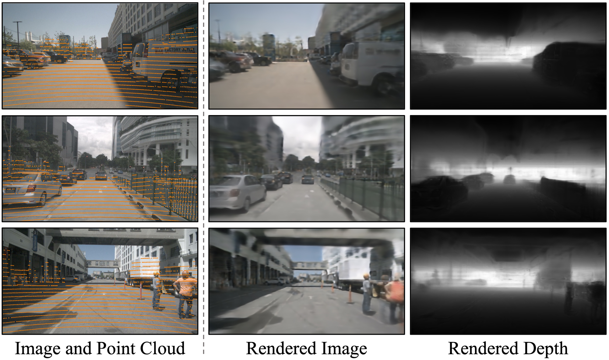
Figure 9: Illustration of the rendering results. The ground truth RGB and projected point clouds, rendered RGB, and rendered depth are shown on the left, middle, and right, respectively.

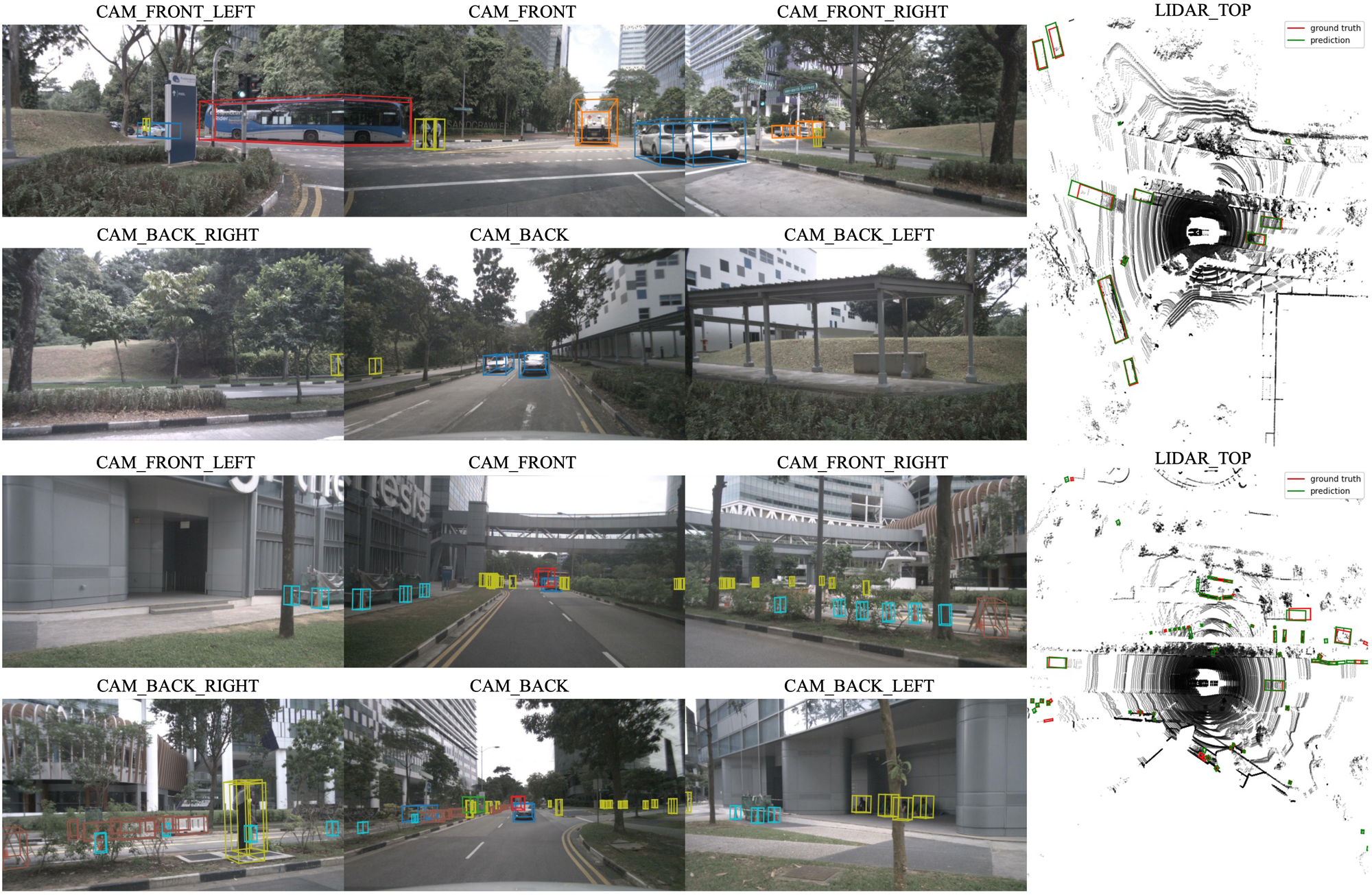
Figure 10: Illustration of the detection results. The predictions are shown on multi-view images and bird’s eye view with LiDAR points.

Masking Ratio Table XXII shows the influence of the masking ratio for the camera modality. We discover that a masking ratio of 0.3, which is lower than the ratios used in previous MAE-based methods, is optimal for our method. This discrepancy could be attributed to the challenge of rendering the original image from the volume representation, which is more complex compared to image-to-image reconstruction. For the point modality, we adopt a mask ratio of 0.8, as suggested in [46], considering the spatial redundancy inherent in point clouds.

Rendering Design Our examinations in Tables XXII, XXIV, and XXIV illustrate the flexible design of our differentiable rendering. In Table XXII, we vary the depth $(D_{\mathrm{SDF}},D_{\mathrm{RGB}})$ of the SDF and RGB decoders, revealing the importance of sufficient decoder depth for succeeding in downstream detection tasks. This is because deeper ones may have the ability to adequately integrate geometry or appearance cues during pre-training. Conversely, as reflected in Table XXIV, the width of the decoder has a relatively minimal impact on performance. Thus, the default dimension is set to $32$ for efficiency. Additionally, we explore the effect of various rendering techniques in Table XXIV, which employ different ways for ray point sampling and accumulation. Using NeuS [65] for rendering records a 0.4 and 0.1 NDS improvement compared to UniSurf [66] and VolSDF [139] respectively, showcasing the learned representation can be improved by utilizing well-designed rendering methods and benefiting from the advancements in neural rendering.

5.7 Qualitative Results

Figure 9 provides some qualitative results of the rendered image and depth map. Our approach has the capability to estimate the depth of small objects, such as cars at a distance. This quality in the pre-training process indicates that our method could encode intricate and continuous geometric representations, which would benefit the downstream tasks. In Figure 10, we present 3D detection results in camera space and BEV (Bird’s Eye View) space with LiDAR point clouds. Our model can predict accurate bounding boxes for nearby objects and also shows the capability of detecting objects from far distances.

6 Conclusions, Limitations and Future Work

In this paper, we propose a novel universal pre-training paradigm for 3D representation learning, which utilizes differentiable neural rendering as the pre-text task. Our method, named PonderV2, can significantly boost over 9 downstream indoor/outdoor tasks including both high-level perception and low-level reconstruction tasks. We have also achieved SOTA performance on over 11 benchmarks. Extensive experiments have shown the flexibility and effectiveness of the proposed method.

Despite the encouraging results, this paper still serves as a start-up work on 3D foundation model. We only show the effectiveness of our pre-training paradigm on a light-weight and efficient backbone, i.e. SparseUNet. It is worth scaling up both the dataset and backbone size to evaluate the extreme boundary of PonderV2 and judge whether or to what extend it can lead to 3D foundation model. Besides, it is also interesting to sufficiently test PonderV2 on more downstream tasks such as reconstruction and robotic control tasks. This may further expand the application scope of 3D representation pre-training. Moreover, neural rendering is a bridge between 3D and 3D worlds. Thus, combining a 2D foundation model with 3D pre-training through techniques such as semantic rendering is valuable. We hope our work can help the building of 3D foundation models in the future.

References

- [1] A. Radford, K. Narasimhan, T. Salimans, I. Sutskever et al., “Improving language understanding by generative pre-training,” OpenAI, 2018.
- [2] A. Radford, J. Wu, R. Child, D. Luan, D. Amodei, I. Sutskever et al., “Language models are unsupervised multitask learners,” OpenAI blog, vol. 1, no. 8, p. 9, 2019.
- [3] T. Brown, B. Mann, N. Ryder, M. Subbiah, J. D. Kaplan, P. Dhariwal, A. Neelakantan, P. Shyam, G. Sastry, A. Askell et al., “Language models are few-shot learners,” Advances in neural information processing systems, vol. 33, pp. 1877–1901, 2020.
- [4] H. Touvron, T. Lavril, G. Izacard, X. Martinet, M.-A. Lachaux, T. Lacroix, B. Rozière, N. Goyal, E. Hambro, F. Azhar et al., “Llama: Open and efficient foundation language models,” arXiv preprint arXiv:2302.13971, 2023.
- [5] H. Touvron, L. Martin, K. Stone, P. Albert, A. Almahairi, Y. Babaei, N. Bashlykov, S. Batra, P. Bhargava, S. Bhosale et al., “Llama 2: Open foundation and fine-tuned chat models,” arXiv preprint arXiv:2307.09288, 2023.
- [6] A. Chowdhery, S. Narang, J. Devlin, M. Bosma, G. Mishra, A. Roberts, P. Barham, H. W. Chung, C. Sutton, S. Gehrmann et al., “Palm: Scaling language modeling with pathways,” arXiv preprint arXiv:2204.02311, 2022.
- [7] I. Team, “Internlm: A multilingual language model with progressively enhanced capabilities,” https://github.com/InternLM/InternLM-techreport, 2023.
- [8] A. Kirillov, E. Mintun, N. Ravi, H. Mao, C. Rolland, L. Gustafson, T. Xiao, S. Whitehead, A. C. Berg, W.-Y. Lo et al., “Segment anything,” arXiv preprint arXiv:2304.02643, 2023.
- [9] R. Rombach, A. Blattmann, D. Lorenz, P. Esser, and B. Ommer, “High-resolution image synthesis with latent diffusion models,” in Proceedings of the IEEE/CVF conference on computer vision and pattern recognition, 2022, pp. 10 684–10 695.
- [10] W. Wang, J. Dai, Z. Chen, Z. Huang, Z. Li, X. Zhu, X. Hu, T. Lu, L. Lu, H. Li et al., “Internimage: Exploring large-scale vision foundation models with deformable convolutions,” in Proceedings of the IEEE/CVF Conference on Computer Vision and Pattern Recognition, 2023, pp. 14 408–14 419.
- [11] Y. Wang, K. Li, Y. Li, Y. He, B. Huang, Z. Zhao, H. Zhang, J. Xu, Y. Liu, Z. Wang et al., “Internvideo: General video foundation models via generative and discriminative learning,” arXiv preprint arXiv:2212.03191, 2022.
- [12] K. He, X. Chen, S. Xie, Y. Li, P. Dollár, and R. Girshick, “Masked autoencoders are scalable vision learners,” in Proceedings of the IEEE/CVF conference on computer vision and pattern recognition, 2022, pp. 16 000–16 009.
- [13] A. Radford, J. W. Kim, C. Hallacy, A. Ramesh, G. Goh, S. Agarwal, G. Sastry, A. Askell, P. Mishkin, J. Clark et al., “Learning transferable visual models from natural language supervision,” in International conference on machine learning. PMLR, 2021, pp. 8748–8763.
- [14] J. Yu, Z. Wang, V. Vasudevan, L. Yeung, M. Seyedhosseini, and Y. Wu, “Coca: Contrastive captioners are image-text foundation models,” arXiv preprint arXiv:2205.01917, 2022.
- [15] P. Zhang, X. D. B. Wang, Y. Cao, C. Xu, L. Ouyang, Z. Zhao, S. Ding, S. Zhang, H. Duan, H. Yan et al., “Internlm-xcomposer: A vision-language large model for advanced text-image comprehension and composition,” arXiv preprint arXiv:2309.15112, 2023.
- [16] X. Chen, X. Wang, S. Changpinyo, A. Piergiovanni, P. Padlewski, D. Salz, S. Goodman, A. Grycner, B. Mustafa, L. Beyer et al., “Pali: A jointly-scaled multilingual language-image model,” arXiv preprint arXiv:2209.06794, 2022.
- [17] J.-B. Alayrac, J. Donahue, P. Luc, A. Miech, I. Barr, Y. Hasson, K. Lenc, A. Mensch, K. Millican, M. Reynolds et al., “Flamingo: a visual language model for few-shot learning,” Advances in Neural Information Processing Systems, vol. 35, pp. 23 716–23 736, 2022.
- [18] J. Li, D. Li, C. Xiong, and S. Hoi, “Blip: Bootstrapping language-image pre-training for unified vision-language understanding and generation,” in International Conference on Machine Learning. PMLR, 2022, pp. 12 888–12 900.
- [19] Y. Li, H. Fan, R. Hu, C. Feichtenhofer, and K. He, “Scaling language-image pre-training via masking,” in Proceedings of the IEEE/CVF Conference on Computer Vision and Pattern Recognition, 2023, pp. 23 390–23 400.
- [20] D. Driess, F. Xia, M. S. M. Sajjadi, C. Lynch, A. Chowdhery, B. Ichter, A. Wahid, J. Tompson, Q. Vuong, T. Yu, W. Huang, Y. Chebotar, P. Sermanet, D. Duckworth, S. Levine, V. Vanhoucke, K. Hausman, M. Toussaint, K. Greff, A. Zeng, I. Mordatch, and P. Florence, “Palm-e: An embodied multimodal language model,” in arXiv preprint arXiv:2303.03378, 2023.
- [21] L. Fan, G. Wang, Y. Jiang, A. Mandlekar, Y. Yang, H. Zhu, A. Tang, D.-A. Huang, Y. Zhu, and A. Anandkumar, “Minedojo: Building open-ended embodied agents with internet-scale knowledge,” Advances in Neural Information Processing Systems, vol. 35, pp. 18 343–18 362, 2022.
- [22] A. Brohan, N. Brown, J. Carbajal, Y. Chebotar, J. Dabis, C. Finn, K. Gopalakrishnan, K. Hausman, A. Herzog, J. Hsu et al., “Rt-1: Robotics transformer for real-world control at scale,” arXiv preprint arXiv:2212.06817, 2022.
- [23] A. Brohan, N. Brown, J. Carbajal, Y. Chebotar, X. Chen, K. Choromanski, T. Ding, D. Driess, A. Dubey, C. Finn et al., “Rt-2: Vision-language-action models transfer web knowledge to robotic control,” arXiv preprint arXiv:2307.15818, 2023.
- [24] H.-S. Fang, H. Fang, Z. Tang, J. Liu, J. Wang, H. Zhu, and C. Lu, “Rh20t: A robotic dataset for learning diverse skills in one-shot,” arXiv preprint arXiv:2307.00595, 2023.
- [25] S. Xie, J. Gu, D. Guo, C. R. Qi, L. Guibas, and O. Litany, “Pointcontrast: Unsupervised pre-training for 3d point cloud understanding,” in Computer Vision–ECCV 2020: 16th European Conference, Glasgow, UK, August 23–28, 2020, Proceedings, Part III 16. Springer, 2020, pp. 574–591.
- [26] J. Hou, B. Graham, M. Nießner, and S. Xie, “Exploring data-efficient 3d scene understanding with contrastive scene contexts,” in Proceedings of the IEEE/CVF Conference on Computer Vision and Pattern Recognition, 2021, pp. 15 587–15 597.
- [27] L. Jiang, S. Shi, Z. Tian, X. Lai, S. Liu, C.-W. Fu, and J. Jia, “Guided point contrastive learning for semi-supervised point cloud semantic segmentation,” in Proceedings of the IEEE/CVF international conference on computer vision, 2021, pp. 6423–6432.
- [28] S. Huang, Y. Xie, S.-C. Zhu, and Y. Zhu, “Spatio-temporal self-supervised representation learning for 3d point clouds,” in Proceedings of the IEEE/CVF International Conference on Computer Vision, 2021, pp. 6535–6545.
- [29] Y. Chen, M. Nießner, and A. Dai, “4dcontrast: Contrastive learning with dynamic correspondences for 3d scene understanding,” in European Conference on Computer Vision. Springer, 2022, pp. 543–560.
- [30] Y. Rao, B. Liu, Y. Wei, J. Lu, C.-J. Hsieh, and J. Zhou, “Randomrooms: Unsupervised pre-training from synthetic shapes and randomized layouts for 3d object detection,” in Proceedings of the IEEE/CVF International Conference on Computer Vision, 2021, pp. 3283–3292.
- [31] Z. Zhang, R. Girdhar, A. Joulin, and I. Misra, “Self-supervised pretraining of 3d features on any point-cloud,” in Proceedings of the IEEE/CVF International Conference on Computer Vision, 2021, pp. 10 252–10 263.
- [32] H. Wang, Q. Liu, X. Yue, J. Lasenby, and M. J. Kusner, “Unsupervised point cloud pre-training via occlusion completion,” in Proceedings of the IEEE/CVF international conference on computer vision, 2021, pp. 9782–9792.
- [33] X. Yu, L. Tang, Y. Rao, T. Huang, J. Zhou, and J. Lu, “Point-bert: Pre-training 3d point cloud transformers with masked point modeling,” in Proceedings of the IEEE/CVF Conference on Computer Vision and Pattern Recognition, 2022, pp. 19 313–19 322.
- [34] S. Yan, Z. Yang, H. Li, C. Song, L. Guan, H. Kang, G. Hua, and Q. Huang, “Implicit autoencoder for point-cloud self-supervised representation learning,” in Proceedings of the IEEE/CVF International Conference on Computer Vision, 2023, pp. 14 530–14 542.
- [35] Y. Pang, W. Wang, F. E. Tay, W. Liu, Y. Tian, and L. Yuan, “Masked autoencoders for point cloud self-supervised learning,” in European conference on computer vision. Springer, 2022, pp. 604–621.
- [36] H. Liu, M. Cai, and Y. J. Lee, “Masked discrimination for self-supervised learning on point clouds,” in European Conference on Computer Vision. Springer, 2022, pp. 657–675.
- [37] R. Zhang, Z. Guo, P. Gao, R. Fang, B. Zhao, D. Wang, Y. Qiao, and H. Li, “Point-m2ae: multi-scale masked autoencoders for hierarchical point cloud pre-training,” Advances in neural information processing systems, vol. 35, pp. 27 061–27 074, 2022.
- [38] C. Min, D. Zhao, L. Xiao, Y. Nie, and B. Dai, “Voxel-mae: Masked autoencoders for pre-training large-scale point clouds,” arXiv preprint arXiv:2206.09900, 2022.
- [39] C. Feichtenhofer, Y. Li, K. He et al., “Masked autoencoders as spatiotemporal learners,” Advances in neural information processing systems, vol. 35, pp. 35 946–35 958, 2022.
- [40] Z. Tong, Y. Song, J. Wang, and L. Wang, “Videomae: Masked autoencoders are data-efficient learners for self-supervised video pre-training,” Advances in neural information processing systems, vol. 35, pp. 10 078–10 093, 2022.
- [41] D. Huang, S. Peng, T. He, H. Yang, X. Zhou, and W. Ouyang, “Ponder: Point cloud pre-training via neural rendering,” in Proceedings of the IEEE/CVF International Conference on Computer Vision, 2023, pp. 16 089–16 098.
- [42] C. Choy, J. Gwak, and S. Savarese, “4d spatio-temporal convnets: Minkowski convolutional neural networks,” in Proceedings of the IEEE/CVF conference on computer vision and pattern recognition, 2019, pp. 3075–3084.
- [43] K. He, H. Fan, Y. Wu, S. Xie, and R. Girshick, “Momentum contrast for unsupervised visual representation learning,” in Proceedings of the IEEE/CVF conference on computer vision and pattern recognition, 2020, pp. 9729–9738.
- [44] T. Chen, S. Kornblith, M. Norouzi, and G. Hinton, “A simple framework for contrastive learning of visual representations,” in International conference on machine learning. PMLR, 2020, pp. 1597–1607.
- [45] X. Wu, X. Wen, X. Liu, and H. Zhao, “Masked scene contrast: A scalable framework for unsupervised 3d representation learning,” in Proceedings of the IEEE/CVF Conference on Computer Vision and Pattern Recognition, 2023, pp. 9415–9424.
- [46] H. Yang, T. He, J. Liu, H. Chen, B. Wu, B. Lin, X. He, and W. Ouyang, “Gd-mae: generative decoder for mae pre-training on lidar point clouds,” in Proceedings of the IEEE/CVF Conference on Computer Vision and Pattern Recognition, 2023, pp. 9403–9414.
- [47] A. Boulch, C. Sautier, B. Michele, G. Puy, and R. Marlet, “Also: Automotive lidar self-supervision by occupancy estimation,” in Proceedings of the IEEE/CVF Conference on Computer Vision and Pattern Recognition, 2023, pp. 13 455–13 465.
- [48] R. Bachmann, D. Mizrahi, A. Atanov, and A. Zamir, “Multimae: Multi-modal multi-task masked autoencoders,” in European Conference on Computer Vision. Springer, 2022, pp. 348–367.
- [49] H. Bao, L. Dong, S. Piao, and F. Wei, “Beit: Bert pre-training of image transformers,” arXiv preprint arXiv:2106.08254, 2021.
- [50] X. Chen, H. Fan, R. Girshick, and K. He, “Improved baselines with momentum contrastive learning,” arXiv preprint arXiv:2003.04297, 2020.
- [51] P. Gao, T. Ma, H. Li, Z. Lin, J. Dai, and Y. Qiao, “Convmae: Masked convolution meets masked autoencoders,” arXiv preprint arXiv:2205.03892, 2022.
- [52] K. Tian, Y. Jiang, Q. Diao, C. Lin, L. Wang, and Z. Yuan, “Designing bert for convolutional networks: Sparse and hierarchical masked modeling,” arXiv preprint arXiv:2301.03580, 2023.
- [53] J. Deng, W. Dong, R. Socher, L.-J. Li, K. Li, and L. Fei-Fei, “Imagenet: A large-scale hierarchical image database,” in 2009 IEEE conference on computer vision and pattern recognition. Ieee, 2009, pp. 248–255.
- [54] Y. Liu, T. Wang, X. Zhang, and J. Sun, “Petr: Position embedding transformation for multi-view 3d object detection,” in European Conference on Computer Vision. Springer, 2022, pp. 531–548.
- [55] H. Liu, Y. Teng, T. Lu, H. Wang, and L. Wang, “Sparsebev: High-performance sparse 3d object detection from multi-camera videos,” in Proceedings of the IEEE/CVF International Conference on Computer Vision, 2023, pp. 18 580–18 590.
- [56] T. Liang, H. Xie, K. Yu, Z. Xia, Z. Lin, Y. Wang, T. Tang, B. Wang, and Z. Tang, “Bevfusion: A simple and robust lidar-camera fusion framework,” Advances in Neural Information Processing Systems, vol. 35, pp. 10 421–10 434, 2022.
- [57] Y. Li, Y. Chen, X. Qi, Z. Li, J. Sun, and J. Jia, “Unifying voxel-based representation with transformer for 3d object detection,” Advances in Neural Information Processing Systems, vol. 35, pp. 18 442–18 455, 2022.
- [58] J. Yan, Y. Liu, J. Sun, F. Jia, S. Li, T. Wang, and X. Zhang, “Cross modal transformer via coordinates encoding for 3d object dectection,” arXiv preprint arXiv:2301.01283, 2023.
- [59] H. Yang, Z. Liu, X. Wu, W. Wang, W. Qian, X. He, and D. Cai, “Graph r-cnn: Towards accurate 3d object detection with semantic-decorated local graph,” in European Conference on Computer Vision. Springer, 2022, pp. 662–679.
- [60] D. Park, R. Ambrus, V. Guizilini, J. Li, and A. Gaidon, “Is pseudo-lidar needed for monocular 3d object detection?” in Proceedings of the IEEE/CVF International Conference on Computer Vision, 2021, pp. 3142–3152.
- [61] T. Wang, X. Zhu, J. Pang, and D. Lin, “Fcos3d: Fully convolutional one-stage monocular 3d object detection,” in Proceedings of the IEEE/CVF International Conference on Computer Vision, 2021, pp. 913–922.
- [62] B. Mildenhall, P. P. Srinivasan, M. Tancik, J. T. Barron, R. Ramamoorthi, and R. Ng, “Nerf: Representing scenes as neural radiance fields for view synthesis,” Communications of the ACM, vol. 65, no. 1, pp. 99–106, 2021.
- [63] T. Müller, A. Evans, C. Schied, and A. Keller, “Instant neural graphics primitives with a multiresolution hash encoding,” ACM Transactions on Graphics (ToG), vol. 41, no. 4, pp. 1–15, 2022.
- [64] A. Yu, R. Li, M. Tancik, H. Li, R. Ng, and A. Kanazawa, “Plenoctrees for real-time rendering of neural radiance fields,” in Proceedings of the IEEE/CVF International Conference on Computer Vision, 2021, pp. 5752–5761.
- [65] P. Wang, L. Liu, Y. Liu, C. Theobalt, T. Komura, and W. Wang, “Neus: Learning neural implicit surfaces by volume rendering for multi-view reconstruction,” arXiv preprint arXiv:2106.10689, 2021.
- [66] M. Oechsle, S. Peng, and A. Geiger, “Unisurf: Unifying neural implicit surfaces and radiance fields for multi-view reconstruction,” in Proceedings of the IEEE/CVF International Conference on Computer Vision, 2021, pp. 5589–5599.
- [67] A. Yu, V. Ye, M. Tancik, and A. Kanazawa, “pixelnerf: Neural radiance fields from one or few images,” in Proceedings of the IEEE/CVF Conference on Computer Vision and Pattern Recognition, 2021, pp. 4578–4587.
- [68] Q. Wang, Z. Wang, K. Genova, P. P. Srinivasan, H. Zhou, J. T. Barron, R. Martin-Brualla, N. Snavely, and T. Funkhouser, “Ibrnet: Learning multi-view image-based rendering,” in Proceedings of the IEEE/CVF Conference on Computer Vision and Pattern Recognition, 2021, pp. 4690–4699.
- [69] K. Zhang, G. Riegler, N. Snavely, and V. Koltun, “Nerf++: Analyzing and improving neural radiance fields,” arXiv preprint arXiv:2010.07492, 2020.
- [70] C. Reiser, S. Peng, Y. Liao, and A. Geiger, “Kilonerf: Speeding up neural radiance fields with thousands of tiny mlps,” in Proceedings of the IEEE/CVF International Conference on Computer Vision, 2021, pp. 14 335–14 345.
- [71] J. T. Barron, B. Mildenhall, M. Tancik, P. Hedman, R. Martin-Brualla, and P. P. Srinivasan, “Mip-nerf: A multiscale representation for anti-aliasing neural radiance fields,” in Proceedings of the IEEE/CVF International Conference on Computer Vision, 2021, pp. 5855–5864.
- [72] W. Xing, J. Chen, and Y. Guo, “Robust local light field synthesis via occlusion-aware sampling and deep visual feature fusion,” Machine Intelligence Research, vol. 20, no. 3, pp. 408–420, 2023.
- [73] K.-A. Aliev, A. Sevastopolsky, M. Kolos, D. Ulyanov, and V. Lempitsky, “Neural point-based graphics,” in Computer Vision–ECCV 2020: 16th European Conference, Glasgow, UK, August 23–28, 2020, Proceedings, Part XXII 16. Springer, 2020, pp. 696–712.
- [74] R. Rakhimov, A.-T. Ardelean, V. Lempitsky, and E. Burnaev, “Npbg++: Accelerating neural point-based graphics,” in Proceedings of the IEEE/CVF Conference on Computer Vision and Pattern Recognition, 2022, pp. 15 969–15 979.
- [75] Q. Xu, Z. Xu, J. Philip, S. Bi, Z. Shu, K. Sunkavalli, and U. Neumann, “Point-nerf: Point-based neural radiance fields,” in Proceedings of the IEEE/CVF Conference on Computer Vision and Pattern Recognition, 2022, pp. 5438–5448.
- [76] H. Zhu, H.-S. Fang, and C. Lu, “X-nerf: Explicit neural radiance field for multi-scene 360∘ insufficient rgb-d views,” arXiv preprint arXiv:2210.05135, 2022.
- [77] J. Ho, A. Jain, and P. Abbeel, “Denoising diffusion probabilistic models,” Advances in neural information processing systems, vol. 33, pp. 6840–6851, 2020.
- [78] A. Dai, A. X. Chang, M. Savva, M. Halber, T. Funkhouser, and M. Nießner, “Scannet: Richly-annotated 3d reconstructions of indoor scenes,” in Proceedings of the IEEE conference on computer vision and pattern recognition, 2017, pp. 5828–5839.
- [79] C. R. Qi, O. Litany, K. He, and L. J. Guibas, “Deep hough voting for 3d object detection in point clouds,” in proceedings of the IEEE/CVF International Conference on Computer Vision, 2019, pp. 9277–9286.
- [80] I. Loshchilov and F. Hutter, “Decoupled weight decay regularization,” arXiv preprint arXiv:1711.05101, 2017.
- [81] I. Misra, R. Girdhar, and A. Joulin, “An end-to-end transformer model for 3d object detection,” in Proceedings of the IEEE/CVF International Conference on Computer Vision, 2021, pp. 2906–2917.
- [82] R. Yamada, H. Kataoka, N. Chiba, Y. Domae, and T. Ogata, “Point cloud pre-training with natural 3d structures,” in Proceedings of the IEEE/CVF Conference on Computer Vision and Pattern Recognition, 2022, pp. 21 283–21 293.
- [83] Z. Zhang, B. Sun, H. Yang, and Q. Huang, “H3dnet: 3d object detection using hybrid geometric primitives,” in Computer Vision–ECCV 2020: 16th European Conference, Glasgow, UK, August 23–28, 2020, Proceedings, Part XII 16. Springer, 2020, pp. 311–329.
- [84] S. Song, S. P. Lichtenberg, and J. Xiao, “Sun rgb-d: A rgb-d scene understanding benchmark suite,” in Proceedings of the IEEE conference on computer vision and pattern recognition, 2015, pp. 567–576.
- [85] S. Peng, M. Niemeyer, L. Mescheder, M. Pollefeys, and A. Geiger, “Convolutional occupancy networks,” in Computer Vision–ECCV 2020: 16th European Conference, Glasgow, UK, August 23–28, 2020, Proceedings, Part III 16. Springer, 2020, pp. 523–540.
- [86] J. Chibane, T. Alldieck, and G. Pons-Moll, “Implicit functions in feature space for 3d shape reconstruction and completion,” in Proceedings of the IEEE/CVF conference on computer vision and pattern recognition, 2020, pp. 6970–6981.
- [87] L. Liu, J. Gu, K. Zaw Lin, T.-S. Chua, and C. Theobalt, “Neural sparse voxel fields,” Advances in Neural Information Processing Systems, vol. 33, pp. 15 651–15 663, 2020.
- [88] A. X. Chang, T. Funkhouser, L. Guibas, P. Hanrahan, Q. Huang, Z. Li, S. Savarese, M. Savva, S. Song, H. Su et al., “Shapenet: An information-rich 3d model repository,” arXiv preprint arXiv:1512.03012, 2015.
- [89] M. Tatarchenko, S. R. Richter, R. Ranftl, Z. Li, V. Koltun, and T. Brox, “What do single-view 3d reconstruction networks learn?” in Proceedings of the IEEE/CVF conference on computer vision and pattern recognition, 2019, pp. 3405–3414.
- [90] C. R. Qi, L. Yi, H. Su, and L. J. Guibas, “Pointnet++: Deep hierarchical feature learning on point sets in a metric space,” Advances in neural information processing systems, vol. 30, 2017.
- [91] H. Thomas, C. R. Qi, J.-E. Deschaud, B. Marcotegui, F. Goulette, and L. J. Guibas, “Kpconv: Flexible and deformable convolution for point clouds,” in Proceedings of the IEEE/CVF international conference on computer vision, 2019, pp. 6411–6420.
- [92] B. Graham, M. Engelcke, and L. Van Der Maaten, “3d semantic segmentation with submanifold sparse convolutional networks,” in Proceedings of the IEEE conference on computer vision and pattern recognition, 2018, pp. 9224–9232.
- [93] H. Zhao, L. Jiang, J. Jia, P. H. Torr, and V. Koltun, “Point transformer,” in Proceedings of the IEEE/CVF international conference on computer vision, 2021, pp. 16 259–16 268.
- [94] R. Jensen, A. Dahl, G. Vogiatzis, E. Tola, and H. Aanæs, “Large scale multi-view stereopsis evaluation,” in Proceedings of the IEEE conference on computer vision and pattern recognition, 2014, pp. 406–413.
- [95] X. Long, C. Lin, P. Wang, T. Komura, and W. Wang, “Sparseneus: Fast generalizable neural surface reconstruction from sparse views,” in European Conference on Computer Vision. Springer, 2022, pp. 210–227.
- [96] W. E. Lorensen and H. E. Cline, “Marching cubes: A high resolution 3d surface construction algorithm,” in Seminal graphics: pioneering efforts that shaped the field, 1998, pp. 347–353.
- [97] D. Rozenberszki, O. Litany, and A. Dai, “Language-grounded indoor 3d semantic segmentation in the wild,” in European Conference on Computer Vision. Springer, 2022, pp. 125–141.
- [98] I. Armeni, O. Sener, A. R. Zamir, H. Jiang, I. Brilakis, M. Fischer, and S. Savarese, “3d semantic parsing of large-scale indoor spaces,” in Proceedings of the IEEE conference on computer vision and pattern recognition, 2016, pp. 1534–1543.
- [99] X. Lai, J. Liu, L. Jiang, L. Wang, H. Zhao, S. Liu, X. Qi, and J. Jia, “Stratified transformer for 3d point cloud segmentation,” in Proceedings of the IEEE/CVF Conference on Computer Vision and Pattern Recognition, 2022, pp. 8500–8509.
- [100] G. Qian, Y. Li, H. Peng, J. Mai, H. Hammoud, M. Elhoseiny, and B. Ghanem, “Pointnext: Revisiting pointnet++ with improved training and scaling strategies,” Advances in Neural Information Processing Systems, vol. 35, pp. 23 192–23 204, 2022.
- [101] X. Wu, Y. Lao, L. Jiang, X. Liu, and H. Zhao, “Point transformer v2: Grouped vector attention and partition-based pooling,” Advances in Neural Information Processing Systems, vol. 35, pp. 33 330–33 342, 2022.
- [102] X. Wu, Z. Tian, X. Wen, B. Peng, X. Liu, K. Yu, and H. Zhao, “Towards large-scale 3d representation learning with multi-dataset point prompt training,” arXiv preprint arXiv:2308.09718, 2023.
- [103] S. Contributors, “Spconv: Spatially sparse convolution library,” https://github.com/traveller59/spconv, 2022.
- [104] I. Armeni, S. Sax, A. R. Zamir, and S. Savarese, “Joint 2d-3d-semantic data for indoor scene understanding,” arXiv preprint arXiv:1702.01105, 2017.
- [105] J. Zheng, J. Zhang, J. Li, R. Tang, S. Gao, and Z. Zhou, “Structured3d: A large photo-realistic dataset for structured 3d modeling,” in Computer Vision–ECCV 2020: 16th European Conference, Glasgow, UK, August 23–28, 2020, Proceedings, Part IX 16. Springer, 2020, pp. 519–535.
- [106] P. Contributors, “Pointcept: A codebase for point cloud perception research,” https://github.com/Pointcept/Pointcept, 2023.
- [107] L. N. Smith and N. Topin, “Super-convergence: Very fast training of neural networks using large learning rates,” in Artificial intelligence and machine learning for multi-domain operations applications, vol. 11006. SPIE, 2019, pp. 369–386.
- [108] L. Jiang, H. Zhao, S. Shi, S. Liu, C.-W. Fu, and J. Jia, “Pointgroup: Dual-set point grouping for 3d instance segmentation,” in Proceedings of the IEEE/CVF conference on computer vision and Pattern recognition, 2020, pp. 4867–4876.
- [109] C.-Y. Wu, J. Johnson, J. Malik, C. Feichtenhofer, and G. Gkioxari, “Multiview compressive coding for 3d reconstruction,” in Proceedings of the IEEE/CVF Conference on Computer Vision and Pattern Recognition, 2023, pp. 9065–9075.
- [110] J. Reizenstein, R. Shapovalov, P. Henzler, L. Sbordone, P. Labatut, and D. Novotny, “Common objects in 3d: Large-scale learning and evaluation of real-life 3d category reconstruction,” in Proceedings of the IEEE/CVF International Conference on Computer Vision, 2021, pp. 10 901–10 911.
- [111] H. Caesar, V. Bankiti, A. H. Lang, S. Vora, V. E. Liong, Q. Xu, A. Krishnan, Y. Pan, G. Baldan, and O. Beijbom, “nuscenes: A multimodal dataset for autonomous driving,” in Proceedings of the IEEE/CVF conference on computer vision and pattern recognition, 2020, pp. 11 621–11 631.
- [112] M. Contributors, “MMDetection3D: OpenMMLab next-generation platform for general 3D object detection,” https://github.com/open-mmlab/mmdetection3d, 2020.
- [113] Y. Yan, Y. Mao, and B. Li, “Second: Sparsely embedded convolutional detection,” Sensors, vol. 18, no. 10, p. 3337, 2018.
- [114] Z. Liu, H. Mao, C.-Y. Wu, C. Feichtenhofer, T. Darrell, and S. Xie, “A convnet for the 2020s,” in Proceedings of the IEEE/CVF conference on computer vision and pattern recognition, 2022, pp. 11 976–11 986.
- [115] B. Zhu, Z. Jiang, X. Zhou, Z. Li, and G. Yu, “Class-balanced grouping and sampling for point cloud 3d object detection,” arXiv preprint arXiv:1908.09492, 2019.
- [116] H. Yang, W. Wang, M. Chen, B. Lin, T. He, H. Chen, X. He, and W. Ouyang, “Pvt-ssd: Single-stage 3d object detector with point-voxel transformer,” in Proceedings of the IEEE/CVF Conference on Computer Vision and Pattern Recognition, 2023, pp. 13 476–13 487.
- [117] T. Yin, X. Zhou, and P. Krahenbuhl, “Center-based 3d object detection and tracking,” in Proceedings of the IEEE/CVF conference on computer vision and pattern recognition, 2021, pp. 11 784–11 793.
- [118] L. Fan, F. Wang, N. Wang, and Z.-X. ZHANG, “Fully sparse 3d object detection,” Advances in Neural Information Processing Systems, vol. 35, pp. 351–363, 2022.
- [119] Y. Chen, J. Liu, X. Zhang, X. Qi, and J. Jia, “Voxelnext: Fully sparse voxelnet for 3d object detection and tracking,” in Proceedings of the IEEE/CVF Conference on Computer Vision and Pattern Recognition, 2023, pp. 21 674–21 683.
- [120] ——, “Largekernel3d: Scaling up kernels in 3d sparse cnns,” in Proceedings of the IEEE/CVF Conference on Computer Vision and Pattern Recognition, 2023, pp. 13 488–13 498.
- [121] X. Bai, Z. Hu, X. Zhu, Q. Huang, Y. Chen, H. Fu, and C.-L. Tai, “Transfusion: Robust lidar-camera fusion for 3d object detection with transformers,” in Proceedings of the IEEE/CVF conference on computer vision and pattern recognition, 2022, pp. 1090–1099.
- [122] Z. Li, W. Wang, H. Li, E. Xie, C. Sima, T. Lu, Y. Qiao, and J. Dai, “Bevformer: Learning bird’s-eye-view representation from multi-camera images via spatiotemporal transformers,” in European conference on computer vision. Springer, 2022, pp. 1–18.
- [123] S. Doll, R. Schulz, L. Schneider, V. Benzin, M. Enzweiler, and H. P. Lensch, “Spatialdetr: Robust scalable transformer-based 3d object detection from multi-view camera images with global cross-sensor attention,” in European Conference on Computer Vision. Springer, 2022, pp. 230–245.
- [124] J. Lu, Z. Zhou, X. Zhu, H. Xu, and L. Zhang, “Learning ego 3d representation as ray tracing,” in European Conference on Computer Vision. Springer, 2022, pp. 129–144.
- [125] C. Shu, J. Deng, F. Yu, and Y. Liu, “3dppe: 3d point positional encoding for multi-camera 3d object detection transformers,” in Proceedings of the IEEE International Conference on Computer Vision, 2023.
- [126] X. Chen, T. Zhang, Y. Wang, Y. Wang, and H. Zhao, “Futr3d: A unified sensor fusion framework for 3d detection,” in Proceedings of the IEEE/CVF Conference on Computer Vision and Pattern Recognition, 2023, pp. 172–181.
- [127] S. Vora, A. H. Lang, B. Helou, and O. Beijbom, “Pointpainting: Sequential fusion for 3d object detection,” in Proceedings of the IEEE/CVF conference on computer vision and pattern recognition, 2020, pp. 4604–4612.
- [128] T. Yin, X. Zhou, and P. Krähenbühl, “Multimodal virtual point 3d detection,” Advances in Neural Information Processing Systems, vol. 34, pp. 16 494–16 507, 2021.
- [129] Z. Chen, Z. Li, S. Zhang, L. Fang, Q. Jiang, and F. Zhao, “Deformable feature aggregation for dynamic multi-modal 3d object detection,” in European Conference on Computer Vision. Springer, 2022, pp. 628–644.
- [130] Z. Liu, H. Tang, A. Amini, X. Yang, H. Mao, D. L. Rus, and S. Han, “Bevfusion: Multi-task multi-sensor fusion with unified bird’s-eye view representation,” in 2023 IEEE International Conference on Robotics and Automation (ICRA). IEEE, 2023, pp. 2774–2781.
- [131] Z. Yang, J. Chen, Z. Miao, W. Li, X. Zhu, and L. Zhang, “Deepinteraction: 3d object detection via modality interaction,” Advances in Neural Information Processing Systems, vol. 35, pp. 1992–2005, 2022.
- [132] H. Tang, Z. Liu, S. Zhao, Y. Lin, J. Lin, H. Wang, and S. Han, “Searching efficient 3d architectures with sparse point-voxel convolution,” in European conference on computer vision. Springer, 2020, pp. 685–702.
- [133] X. Zhu, H. Zhou, T. Wang, F. Hong, Y. Ma, W. Li, H. Li, and D. Lin, “Cylindrical and asymmetrical 3d convolution networks for lidar segmentation,” in Proceedings of the IEEE/CVF conference on computer vision and pattern recognition, 2021, pp. 9939–9948.
- [134] X. Lai, Y. Chen, F. Lu, J. Liu, and J. Jia, “Spherical transformer for lidar-based 3d recognition,” in Proceedings of the IEEE/CVF Conference on Computer Vision and Pattern Recognition, 2023, pp. 17 545–17 555.
- [135] K. He, G. Gkioxari, P. Dollár, and R. Girshick, “Mask r-cnn,” in Proceedings of the IEEE international conference on computer vision, 2017, pp. 2961–2969.
- [136] Y.-C. Liu, Y.-K. Huang, H.-Y. Chiang, H.-T. Su, Z.-Y. Liu, C.-T. Chen, C.-Y. Tseng, and W. H. Hsu, “Learning from 2d: Contrastive pixel-to-point knowledge transfer for 3d pretraining,” arXiv preprint arXiv:2104.04687, 2021.
- [137] J. Huang, G. Huang, Z. Zhu, Y. Ye, and D. Du, “Bevdet: High-performance multi-camera 3d object detection in bird-eye-view,” arXiv preprint arXiv:2112.11790, 2021.
- [138] Y. Li, Z. Ge, G. Yu, J. Yang, Z. Wang, Y. Shi, J. Sun, and Z. Li, “Bevdepth: Acquisition of reliable depth for multi-view 3d object detection,” in Proceedings of the AAAI Conference on Artificial Intelligence, vol. 37, no. 2, 2023, pp. 1477–1485.
- [139] L. Yariv, J. Gu, Y. Kasten, and Y. Lipman, “Volume rendering of neural implicit surfaces,” Advances in Neural Information Processing Systems, vol. 34, pp. 4805–4815, 2021.