Exact and asymptotic distribution theory for the empirical correlation of two AR(1) processes

Abstract

This paper begins with a study of both the exact distribution and the asymptotic distribution of the empirical correlation of two independent AR(1) processes with Gaussian innovations. We proceed to develop rates of convergence for the distribution of the scaled empirical correlation to the standard Gaussian distribution in both Wasserstein distance and in Kolmogorov distance. Given $n$ data points, we prove the convergence rate in Wasserstein distance is $n^{-1/2}$ and the convergence rate in Kolmogorov distance is $n^{-1/2}\sqrt{\ln n}$. We then compute rates of convergence of the scaled empirical correlation to the standard Gaussian distribution for two additional classes of AR(1) processes: (i) two AR(1) processes with correlated Gaussian increments and (ii) two independent AR(1) processes driven by white noise in the second Wiener chaos.

MSC 2020 Codes Primary: 60G15, 60F05. Secondary: 62M10.

Keywords: Autoregressive processes; Gaussian processes; Kolmogorov distance; Wasserstein distance; Wiener chaos; Yule’s “nonsense correlation.”

1 Introduction.

It is well known that the distribution of the empirical correlation (defined in (1) below) of two independent and identically distributed (i.i.d.) simple random walks is widely dispersed and frequently large in absolute value (see histograms in [7, p.1791]) and [16, p.35]). In addition, the observed correlation has a very different distribution than that of the nominal $t$-distribution. The phenomenon was first (empirically) observed in 1926 by the famed British statistician G. Udny Yule, who called it “nonsense correlation” ([16]). More than ninety years later, Ernst, Shepp, and Wyner ([7]) succeeded in analytically calculating the variance of this distribution to be .240522.
Yule’s “nonsense correlation” provides a stark warning that in the case of two sequences of i.i.d. random walks (or, alternatively two independent standard Wiener processes), that the empirical correlation cannot be used to test independence of the two processes. However, the same may not necessarily be true for other classes of stochastic processes. In 2019, the authors of [5] proved that in the case of two independent Ornstein-Uhlenbeck processes, the scaled empirical correlation asymptotically converges to the Gaussian random variable with mean zero and with variance $\frac{1}{2r}$, where $r$ is the mean reversion parameter of the Ornstein-Uhlenbeck process (see [5, Theorem 4]). Accordingly, and desirably do, the variance tends to zero as the mean reversion parameter tends towards $\infty$. Rates of convergence of the distribution of the empirical correlation of two independent Ornstein-Uhlenbeck processes to the standard Gaussian distribution were studied in 2022 by the authors of [3]. The phenomenon of Yule’s “nonsense correlation” also appears to be absent when considering the empirical correlation of other stochastic processes admitting stationary distributions. For example, one may consider the case of two independent and causal AR(1) processes (for sake of clarity, note that we are invoking the standard definition of “causal” in the time series literature (see, for example, [6, p.1836], and references therein). Therefore, throughout the sequel, we shall assume that we are only considering causal AR(1) processes. It is proven in ([14, Theorem A.8]) that the scaled empirical correlation of two independent AR(1) processes follows an asymptotically normal distribution. Additional literature closely related to the above lines of investigation includes [1, 2, 8].
The first key goal of the present paper is to study the empirical correlation of two independent and causal AR(1) processes. We begin by considering the model of two independent AR(1) processes with Gaussian noise. Formally, let two independent AR(1) processes be defined by

$$\begin{cases}X_{n}=\alpha X_{n-1}+\xi_{n},\quad n\in\mathds{N}_{+}\\ X_{0}=0\end{cases}\text{ and }\begin{cases}Y_{n}=\alpha Y_{n-1}+\eta_{n},\quad n\in\mathds{N}_{+}\\ Y_{0}=0\end{cases},$$

where $|\alpha|<1$ and $\xi_{1},\xi_{2},\xi_{3},\dots$, $\eta_{1},\eta_{2},\eta_{3},\dots$ are independent standard normal random variables. The empirical correlation for the AR(1) processes $\{X_{n}\}_{n=0}^{\infty}$ and $\{Y_{n}\}_{n=0}^{\infty}$ is then defined in the standard way

$$\theta_{n}:=\frac{\frac{1}{n}\sum_{i=1}^{n}X_{i}Y_{i}-\frac{1}{n^{2}}(\sum_{i=1}^{n}X_{i})(\sum_{i=1}^{n}Y_{i})}{\sqrt{\frac{1}{n}\sum_{i=1}^{n}X_{i}^{2}-\frac{1}{n^{2}}(\sum_{i=1}^{n}X_{i})^{2}}\sqrt{\frac{1}{n}\sum_{i=1}^{n}Y_{i}^{2}-\frac{1}{n^{2}}(\sum_{i=1}^{n}Y_{i})^{2}}}.$$ (1)

Section 3 is devoted to the study of the exact distribution of the empirical correlation $\theta_{n}$. We provide the exact distribution of $\theta_{n}$ for all values of $n$. We then use the first $10$ moments of $\theta_{n}$ to approximate the density of the scaled empirical correlation $\sqrt{n}\theta_{n}$. The analysis is based on a symbolically tractable integro-differential representation expression for the moments (of any order) in a class of empirical correlations. This integro-differential representation was first established in [5] and was recently employed in [4]. In order to apply this representation, one must explicitly compute the tri-variate moment generating function of the three empirical sums of products and squares which appear in the empirical correlation $\theta_{n}$. Our strategy to achieve this is to begin by representing the three elements constituting $\theta_{n}$ in quadratic forms in term of the increments $\xi$ and $\eta$. This leads us to obtain the matrix $K_{n}$ (defined in (14)). We then explicitly calculate the “alternative characteristic polynomial” $d_{n}(\lambda)$ (defined in (15)) for the matrix $K_{n}$. This leads to a closed form of the tri-variate moment generating function $\phi_{n}$ of the three elements of $\theta_{n}$. In contrast to the matrix $K_{n}$ considered by the authors of [4]), the matrix $K_{n}$ here is considerably more complex, and indeed none of the techniques developed in [4] can be applied. In computing $d_{n}(\lambda)$, the first key observation is that the matrix $I_{n}-\lambda K_{n}$ can be decomposed as the sum of two matrices. The first matrix (after conducting elementary matrix operations) is an invertible tri-diagonal matrix which exhibits self-similarity (with the exception of one cell) and the second matrix has rank $1$. The determinant of $I_{n}-\lambda K_{n}$ can be expressed in term of determinant and cofactors of the aforementioned tri-diagonal matrix, which can be explicitly derived by solving a second-order recursion formula. The explicit calculation of $d_{n}(\lambda)$ is the key mathematical tool of the present paper. This is because it (i) it is the key ingredient in the calculation of the tri-variate mgf $\phi_{n}$ and (ii) it plays an important role in estimating the negative moments and the moment generating functions of elements constituting the denominator of $\theta_{n}$. The full details of these calculations are revealed in Appendix A.
Section 4 is devoted to the study of the convergence rate of the scaled empirical correlation of two independent AR(1) processes with Gaussian increments to the standard normal distribution. We investigate the convergence rates of the distribution of the scaled empirical correlation (i.e. $\sqrt{n}\theta_{n}$ multiplied by a normalized constant) to the standard normal distribution in both Wasserstein distance and in Kolmogorov distance. We find that the convergence rate in Wasserstein distance is $n^{-1/2}$; in Kolmogorov distance, it is $n^{-1/2}\sqrt{\ln n}$. The derivation of the convergence rate relies upon the estimates of the eigenvalues of $K_{n}$ in Section 4.1, which is extremely delicate and is the most mathematically challenging part of the present paper. In Section 4.2), we consider the convergence of the scaled numerator of $\theta_{n}$ to the standard normal distribution and find the convergence rate of $n^{-1/2}$. This result relies in large part on the work of Nourdin and Peccati [10], who demonstrated that the Kolmogorov distance between the distribution of random variable $X$ in $q$-th Wiener chaos and the standard normal distribution can be bounded by the standard deviation of the difference between $1$ and $q^{-1}$ times the square of the Hilbert-space norm of the Malliavin derivative $DX$. The Nourdin-Peccati result can also be immediately extended to Wasserstein distance and to total variation. For more details, please refer to [11, 12]. Section 4.3 is devoted to utilizing the convergence rate of the scaled numerator of $\theta_{n}$ in order to find the convergence rate of the entire fraction (in both Wasserstein distance and in Kolmogorov distance). The work relies extensively on the explicit expression of the aforementioned alternative characteristic polynomial $d_{n}(\lambda)$. In the case of Wasserstein distance, a key ingredient is developing a uniform upper bound for the negative second moments of the elements of the denominator of $\theta_{n}$. After extensive calculation, we see that this reduces to a uniform lower bound of $(n-1)$ times the product of the positive eigenvalues of $K_{n}$. Due to the explicit expression for the alternative characteristic function $d_{n}(\lambda)$, the product of positive eigenvalues can be calculated explicitly, leading to a uniform lower bound of $(n-1)$ times the product of the positive eigenvalues of $K_{n}$. In the case of Kolmogorov distance, the analysis requires estimation of the tails of the elements within the denominator of $\theta_{n}$. These estimates are obtained through the explicit expressions of their moment generating functions, which can be represented in terms of the alternative characteristic function $d_{n}(\lambda)$. These two parts culminate in a convergence rate of $n^{-1/2}$ for Wasserstein distance and a convergence rate of $n^{-1/2}\sqrt{\ln n}$ for Kolmogorov distance.
In Section 5, we study the distribution and asymptotic behavior of the empirical correlation of two AR(1) processes with correlated Gaussian increments. Formally, two AR(1) processes are correlated with coefficient $r$ if the pairs of increments $(\xi_{n},\eta_{n})$ are i.i.d. Gaussian random vectors with mean zero and covariance matrix

$$\begin{pmatrix}1&r\\ r&1\end{pmatrix},$$

where $|r|\leq 1$. We study the distribution of the empirical correlation by calculating its moments of all orders. Additionally, we find the convergence rate of the scaled empirical correlation to the standard normal to be $n^{-1/2}\sqrt{\ln n}$ in Kolmogorov distance. This proves that the scaled empirical correlation is asymptotically normal with mean $r$. We then proceed to study the statistical power of the test for the region

$$|\sqrt{n}\,\theta_{n}|>c,$$

for any constant $c$.

In Section 6, we extend the scope of our existing study by considering the model of two independent AR(1) processes driven by white noise in the second Wiener chaos, which has the form

$$X_{n}=\alpha X_{n-1}+\xi_{n},$$ (2)

where $\{\xi_{n};n\in\mathds{N}_{+}\}$ is sequence of i.i.d. random variables in the second Wiener chaos, and $\alpha$ is a constant. Recall that random variables are in the second Wiener chaos if they can be expressed as

$$\sum_{i=1}^{\infty}a_{i}\left(Z_{i}^{2}-1\right),$$

where $Z_{i}$ are i.i.d. standard normal random variables and $\sum_{i=1}^{\infty}a_{i}^{2}<\infty$ ([11]). Section 6 includes a complete description and construction of this process and of the noise sequence. We establish that the rate of convergence of the empirical correlation to the standard normal is $n^{-1/2}\sqrt{\ln n}$ in Kolmogorov distance. Note that this rate is the same as that established in both Section 3 and in Section 5. There are two advantages of studying a model with white noise in the second Wiener chaos. The first is theoretical in nature: the second Wiener chaos is a linear space and the solution of (2), which can be represented by linear combination of the noise sequence, still lies in the same chaos. This allows us to use tools from the analysis on Wiener space to establish optimal estimates. The second advantage is practical in nature: the second Wiener chaos contains several distributions commonly utilized to model real world data. The most Gumbel distribution is a second chaos distribution which is often employed by practitioners studying extreme values in environmental time series (see, for example, [15, p.256-257]).

The literature most directly related to the work in Section 6 includes [3] and [5], although neither are concerned with studying the empirical correlation of two AR(1) processes driven by white noise in the second Wiener chaos. The work of [5] studies the asymptotic behavior of the scaled empirical correlation of two independent Ornstein–Uhlenbeck processes, while [3] primarily focuses on rates of convergence. As mentioned above, we find that the rate of convergence in Kolmogorov distance is $n^{-1/2}\sqrt{\ln n}$. This result slightly improves the result presented in [3], where the rate of convergence in Kolmogorov distance is $T^{-1/2}\ln T$; here, $T$ represents the length of the Ornstein–Uhlenbeck process and therefore is analogous to the sample size $n$ for a discrete-time process. We note that the techniques developed in Section 6 of the present paper can be directly applied to improve the convergence rate in [3] to $T^{-1/2}\sqrt{\ln T}$.

The remainder of the paper is organized as follows. In Section 2, we introduce some key elements of analysis on Wiener space, which enable us to work with convergence rates for the scaled numerator of the empirical correlation $\theta_{n}$. We also introduce some necessary notation, including that of the “kernel” matrix $K_{n}$, its “alternative characteristic polynomial” $d_{n}(\lambda)$ and the tri-variate moment generating function $\phi_{n}$. Section 3 is devoted to exact distribution theory of $\theta_{n}$ for the model of two independent AR(1) processes with Gaussian increments. We start by explicitly calculating $d_{n}$ and $\phi_{n}$, and continue with an explicit formula for the second moment of $\sqrt{n}\theta_{n}$ for any $n$. Additionally, we provide numerical results for moments of $\sqrt{n}\theta_{n}$, facilitating the approximation of the density of $\sqrt{n}\theta_{n}$. In Section 4, we study the asymptotic behavior of the empirical correlation for two independent AR(1) processes with Gaussian increments. We also establish the rates of convergence to the standard normal distribution in both Wasserstein distance and Kolmogorov distance. In Section 5, we extend these results to the model of AR(1) processes with correlated Gaussian increments. The paper concludes with Section 6, which investigates the asymptotic behavior of the empirical correlation for the model of two AR(1) processes driven by second Wiener chaos noise.

2 Preliminaries.

This first subsection introduces fundamental tools for analysis on Wiener space. The exposition below very closely follows [3, Section 2] and [1, Section 2]. For further details about analysis on Wiener space, we refer the reader to [11] and [12].

2.1 Fundamental Tools for Analysis on Wiener space

Let $(\Omega,\mathcal{F},P)$ denote the Wiener space of a standard Wiener process $W$ and let the space $\mathcal{H}$ be denoted as

$$\mathcal{H}=L^{2}(\mathbb{R}_{+}).$$

For two deterministic functions $f$ and $g$, the inner product is defined as

$$\langle f,g\rangle_{\mathcal{H}}:=\int_{\mathbb{R}_{+}}f(s)g(s)\,ds.$$

The fundamental elements of analysis on Wiener space employed in the present paper are detailed in the bullet points below.

• Wiener chaos expansion. For all $q\geq 1$, let $\mathcal{H}_{q}$ denote the $q$-th Wiener chaos of $W$. Note that Wiener chaoses of different orders are orthogonal in $L^{2}(\Omega)$. The fact that any $X\in L^{2}(\Omega)$ can be orthogonally decomposed as

  $$X=E[X]+\sum_{q=1}^{\infty}X_{q}$$ (3)

  for some $X_{q}\in\mathcal{H}_{q}$ and for every $q\geq 1$ is known as the “Wiener chaos expansion.”

• Symmetrization and symmetric tensor space. For a mapping $f:\mathbb{R}_{+}^{n}\rightarrow\mathbb{R}$, its symmetrization is given by

  $$\tilde{f}(t_{1},\dots,t_{n})=\frac{1}{n!}\sum_{\sigma}f\left(t_{\sigma(1)},\dots,t_{\sigma(n)}\right),$$

  where the sum is taken over all permutations $\sigma$ of $\{1,2,\dots,n\}$. Let $f\,\widetilde{\otimes}\,g$ denote the symmetrization of the tensor $f\otimes g$. The symmetric tensor space $\mathcal{H}^{\odot q}$ is the linear space of the symmetrization of functions from the tensor space $\mathcal{H}^{\otimes q}$.

• Multiple Wiener integrals. The mapping $\mathcal{I}_{q}$ is the so-called “multiple Wiener integral.” The mapping $\mathcal{I}_{q}$ is a contraction; that is, for any $f\in\mathcal{H}^{\otimes q}$,

  $$\left\lVert\mathcal{I}_{q}(f)\right\rVert_{\mathcal{H}_{q}}\leq\sqrt{q!}\left\lVert f\right\rVert_{\mathcal{H}^{\otimes q}}.$$

  It is useful to note that, for any $f\in\mathcal{H}^{\otimes q}$, $\mathcal{I}_{q}(\tilde{f})=\mathcal{I}_{q}(f).$

  If we consider the symmetric tensor space $\mathcal{H}^{\odot q}$, then $\mathcal{I}_{q}$ is a linear isometry between the symmetric tensor product $\mathcal{H}^{\odot q}$ (equipped with the modified norm $\lVert\cdot\rVert_{\mathcal{H}^{\odot q}}$) and $\mathcal{H}_{q}$. For any nonnegative integers $p$ and $q$, and functions $f\in\mathcal{H}^{\odot p}$ and $g\in\mathcal{H}^{\odot q}$, the formula for the inner product is given by

  $$E\left[\mathcal{I}_{p}(f)\mathcal{I}_{q}(g)\right]=\begin{cases}p!\left\langle f,g\right\rangle_{\mathcal{H}^{\otimes p}}&\quad\text{if $p=q$}\\ 0&\quad\text{otherwise}\end{cases},$$ (4)

  Hence, for both $X$ and its Wiener chaos expansion in (3) above, each term $X_{q}$ is a multiple Wiener integral $\mathcal{I}_{q}(f_{q})$ for some $f_{q}\in\mathcal{H}^{\odot q}$.

• Product formula and contractions. Let $f\in\mathcal{H}^{\otimes p}$ and $g\in\mathcal{H}^{\otimes q}$. For any $r=0,\dots,p\wedge q$, the contraction of $f$ and $g$ of order $r$ is defined as an element in $\mathcal{H}^{\otimes(p+q-2r)}$ and is given by

  $$(f\otimes_{r}g)(s_{1},\dots,s_{p-r},t_{1},\dots,t_{q-r})$$

  $$:= \int_{\mathbb{R}_{+}^{r}}f(s_{1},\dots,s_{p-r},u_{1},\dots,u_{r})\,g(t_{1},\dots,t_{q-r},u_{1},\dots,u_{r})\,du_{1}\cdots du_{r}.$$

  Furthermore, the product of two multiple Wiener integrals satisfies

  $$\mathcal{I}_{p}(f)\mathcal{I}_{q}(g)=\sum_{r=0}^{p\wedge q}r!\binom{p}{r}\binom{q}{r}\mathcal{I}_{p+q-2r}(f\widetilde{\otimes}_{r}g),$$ (5)

  where $f\widetilde{\otimes}_{r}g$ denotes the symmetrization of $f\otimes_{r}g$.

• Hypercontractivity in Wiener chaos. For $q\geq 2$, every random variable in $q$-th Wiener chaos admits the “hypercontractivity property.” The hypercontractivity property implies the equivalence in $\mathcal{H}_{q}$ of all $L^{p}$ norms. In particular, for any $F\in\mathcal{H}_{q}$, and for $1<p<r<\infty$,

  $$\left(E\left[|F|^{r}\right]\right)^{1/r}\leq\left(\frac{r-1}{p-1}\right)^{q/2}\left(E\left[|F|^{p}\right]\right)^{1/p}.$$ (6)

• The Malliavin derivative. Consider a function $\Phi\in C^{1}(\mathbb{R}^{n})$ with bounded derivative. Let $h_{1},\dots,h_{n}\in\mathcal{H}$. Let the Wiener integral $\int_{\mathbb{R}_{+}}h(s)\,dW(s)$ be denoted by $W(h)$. The “Malliavin derivative” $D$ of the random variable $X:=\Phi(W(h_{1}),\dots,W(h_{n}))$ obeys the following chain rule:

  $$DX:X\mapsto D_{s}X:=\sum_{k=1}^{n}\frac{\partial\Phi}{\partial x_{k}}(W(h_{1}),\dots,W(h_{n}))\,h_{k}(s)\in L^{2}(\Omega\times\mathbb{R}_{+}).$$

  One may proceed to extend the Malliavin derivative $D$ to the Gross-Sobolev subset $\mathbb{D}^{1,2}\subsetneqq L^{2}(\Omega)$. This is done by closing $D$ inside $L^{2}(\Omega)$ under the norm

  $$\lVert X\rVert_{1,2}^{2}=E\left[X^{2}\right]+E\left[\int_{\mathbb{R}_{+}}|D_{s}X|^{2}\,ds\right].$$

  A useful fact is that all Wiener chaos random variables are in the domain $\mathbb{D}^{1,2}$ of $D$. For any $X\in L^{2}(\Omega)$ with Wiener chaos expansion $E[X]+\sum_{q}\mathcal{I}_{q}(f_{q}),$ $X\in\mathbb{D}^{1,2}$ if and only if $\sum_{q}qq!\lVert f_{q}\rVert_{\mathcal{H}^{\otimes q}}^{2}<\infty$.

• Generator $L$ of the Ornstein-Uhlenbeck semigroup. The linear operator $L$ is diagonal under the Wiener chaos expansion of $L^{2}(\Omega)$. Further, $\mathcal{H}_{q}$ is the eigenspace of $L$ with eigenvalue $-q$ (or, equivalently, for $X\in\mathcal{H}_{q}$, $LX=-qX$). Finally, the operator $-L^{-1}$ is the negative pseudo-inverse of $L$. This means that for any $X\in\mathcal{H}_{q}$, $-L^{-1}X=q^{-1}X$.

• Kolmogorov distance, Wasserstein distance, and total variation. Let $X$ and $Y$ be two real-valued random variables. We define the Kolmogorov distance between the law of $X$ and the law of $Y$ as

  $$d_{Kol}(X,Y)=\sup_{z\in\mathbb{R}}\left|P(X\leq z)-P(Y\leq z)\right|.$$

  We define the total variation between the law of $X$ and the law of $Y$ by

  $$d_{TV}(X,Y)=\sup_{A\in\mathcal{B}(\mathbb{R})}\left|P(X\in A)-P(Y\in A)\right|,$$ (7)

  where the supremum is taken over all Borel sets on $\mathbb{R}$. If $X$ and $Y$ are integrable, we may define the Wasserstein distance between the law of $X$ and the law of $Y$ by

  $$d_{W}(X,Y)=\sup_{f\in\mathrm{Lip}(1)}\left|Ef(X)-Ef(Y)\right|,$$

  where $\mathrm{Lip}(1)$ is the set of all Lipschitz functions with Lipschitz constant $\leq 1$. Moreover, let $X$ be a mean zero random variable with $X\in\mathbb{D}^{1,2}$ and let the random variable $Y$ be standard normal. The following upper bounds for Kolmogorov distance and Wasserstein distance are given below (see Chapter 8.2, 8.3 in [12] or Theorem 2.4 in [10]):

  $$d_{Kol}(X,Y)\leq\sqrt{E\left[\left(1-\langle DX,-DL^{-1}X\rangle_{\mathcal{H}}\right)^{2}\right]},$$ (8)

  $$d_{W}(X,Y)\leq\sqrt{\frac{2}{\pi}}\sqrt{E\left[\left(1-\langle DX,-DL^{-1}X\rangle_{\mathcal{H}}\right)^{2}\right]},$$ (9)

  $$d_{TV}(X,Y)\leq 2\sqrt{E\left[\left(1-\langle DX,-DL^{-1}X\rangle_{\mathcal{H}}\right)^{2}\right]}.$$ (10)

  Note that if, for all $q\geq 2$, $X\in\mathcal{H}_{q}$ , then $\langle DX,-DL^{-1}X\rangle_{\mathcal{H}}=q^{-1}\lVert DX\rVert_{\mathcal{H}}^{2}$. The following three inequalities hold:

  $$d_{Kol}(X,Y)\leq\sqrt{E\left[\left(1-q^{-1}\lVert DX\rVert_{\mathcal{H}}^{2}\right)^{2}\right]},$$ (11)

  $$d_{W}(X,Y)\leq\sqrt{\frac{2}{\pi}}\sqrt{E\left[\left(1-q^{-1}\lVert DX\rVert_{\mathcal{H}}^{2}\right)^{2}\right]},$$ (12)

  $$d_{TV}(X,Y)\leq 2\sqrt{E\left[\left(1-q^{-1}\lVert DX\rVert_{\mathcal{H}}^{2}\right)^{2}\right]}.$$ (13)

2.2 Notation.

This subsection introduces some necessary notation to be utilized in the sequel. We use $I_{n}$ to denote the $n\times n$ identity matrix. For $n\in\mathds{N}_{+}$, we define the $n\times n$ symmetric matrix $K_{n}$ by

$$K_{n}:=\left\{\frac{1}{n}\,\frac{\alpha^{|k-j|}-\alpha^{k+j}}{1-\alpha^{2}}-\frac{1}{n^{2}}\,\frac{(1-\alpha^{k})(1-\alpha^{j})}{(1-\alpha)^{2}}\right\}_{j,k=1}^{n}.$$ (14)

The “alternative characteristic polynomial” $d_{n}(\lambda)$ for the matrix $K_{n}$ is defined by

$$d_{n}(\lambda)=\det(I_{n}-\lambda K_{n}).$$ (15)

If the the case that the eigenvalues of $K_{n}$ are known, and are denoted by $\lambda_{1},\lambda_{2}\cdots,\lambda_{n}$, the alternative characteristic polynomial can also be expressed as

$$d_{n}(\lambda)=\prod_{j=1}^{n}(1-\lambda_{j}\lambda).$$ (16)

We also define two $n\times 1$ column random vectors $\mathbf{\Xi}_{n}$ and $\mathbf{H}_{n}$ by

$$\mathbf{\Xi}_{n}:=\left(\xi_{n},\xi_{n-1},\dots,\xi_{1}\right)^{\intercal}\quad\text{and}\quad\mathbf{H}_{n}:=\left(\eta_{n},\eta_{n-1},\dots,\eta_{1}\right)^{\intercal},$$

where $\xi_{1},\xi_{2},\xi_{3},\dots$, $\eta_{1},\eta_{2},\eta_{3},\dots$ are independent standard normal random variables. Let

$$Z_{11}^{n}:=\frac{1}{n}\sum_{i=1}^{n}X_{i}^{2}-\frac{1}{n^{2}}\left(\sum_{i=1}^{n}X_{i}\right)^{2},$$ (17)

$$Z_{22}^{n}:=\frac{1}{n}\sum_{i=1}^{n}Y_{i}^{2}-\frac{1}{n^{2}}\left(\sum_{i=1}^{n}Y_{i}\right)^{2},$$ (18)

$$Z_{12}^{n}:=\frac{1}{n}\sum_{i=1}^{n}X_{i}Y_{i}-\frac{1}{n^{2}}\left(\sum_{i=1}^{n}X_{i}\right)\left(\sum_{i=1}^{n}Y_{i}\right).$$ (19)

Combining the above with (1), one can easily check that

$$\theta_{n}=Z_{12}^{n}/\sqrt{Z_{11}^{n}Z_{22}^{n}}.$$

Finally, let us define the joint moment generating function (mgf) of the random vector $\left(Z^{n}_{11},Z^{n}_{12},Z^{n}_{22}\right)$ by

$$\phi_{n}(s_{11},s_{12},s_{22}):=E\left[\exp\left\{-\frac{1}{2}\left(s_{11}Z_{11}^{n}+2s_{12}Z_{12}^{n}+s_{22}Z_{22}^{n}\right)\right\}\right],$$

where $s_{11},s_{12}$ and $s_{22}$ are such that $s_{11},s_{22}\geq 0$ and $s_{12}^{2}\leq s_{11}s_{22}$. These two inequalities ensure that $\phi_{n}(s_{11},s_{12},s_{22})$ is well-defined, as we shall see in Section 3.1.

3 The distribution of $\sqrt{n}\theta_{n}$.

This section is devoted to exact distribution theory of the scaled empirical correlation of two independent AR(1) processes with Gaussian noise. Let two independent AR(1) processes be defined by

$$\begin{cases}X_{n}=\alpha X_{n-1}+\xi_{n},\quad n\in\mathds{N}_{+}\\ X_{0}=0\end{cases}\text{ and }\begin{cases}Y_{n}=\alpha Y_{n-1}+\eta_{n},\quad n\in\mathds{N}_{+}\\ Y_{0}=0\end{cases},$$

where $|\alpha|<1$ and $\xi_{1},\xi_{2},\xi_{3},\dots$, $\eta_{1},\eta_{2},\eta_{3},\dots$ are independent standard normal random variables. We study the empirical correlation (as originally defined in (1) above) for the AR(1) processes $\{X_{n}\}_{n=0}^{\infty}$ and $\{Y_{n}\}_{n=0}^{\infty}$. Our interest is to study the exact distribution of $\sqrt{n}\theta_{n}$ for any fixed $n$ (note that we do not study the distribution of $\theta_{n}$ since $\theta_{n}$ converges to $0$). We begin by calculating the joint moment generating function $\phi_{n}(s_{11},s_{12},s_{22})$, followed by the formulas for moments of $\sqrt{n}\theta_{n}$. We then proceed to approximate the distribution of $\sqrt{n}\theta_{n}$ using its higher-order moments.

3.1 Calculating the joint moment generating function.

In this section, we derive an expression for the joint moment generating function $\phi_{n}(s_{11},s_{12},s_{22})$, which shall serve as the key ingredient for computing the moments of $\theta_{n}$ for all $n$.

By the definition of an AR(1) process, we may easily obtain that, for all $n\in\mathds{N}_{+}$,

$$X_{n}=\sum_{k=1}^{n}\alpha^{n-k}\xi_{k}\quad\text{and}\quad Y_{n}=\sum_{k=1}^{n}\alpha^{n-k}\eta_{k}.$$

Then

$$\sum_{i=1}^{n}X_{i}Y_{i}=\sum_{i=1}^{n}\left(\sum_{k=1}^{i}\alpha^{i-k}\xi_{k}\right)\left(\sum_{j=1}^{i}\alpha^{i-j}\eta_{j}\right)=\sum_{j,k=1}^{n}\,\sum_{i=\max(k,j)}^{n}\alpha^{i-k}\alpha^{i-j}\,\xi_{k}\eta_{j}$$ (20)

$$= \sum_{j,k=1}^{n}\frac{\alpha^{2\times\max(k,j)}-\alpha^{2n+2}}{1-\alpha^{2}}\,\alpha^{-k}\alpha^{-j}\,\xi_{k}\eta_{j}=\sum_{j,k=1}^{n}\frac{\alpha^{|k-j|}-\alpha^{2n+2-k-j}}{1-\alpha^{2}}\,\xi_{k}\eta_{j}.$$

Further,

$$\sum_{i=1}^{n}X_{i}=\sum_{i=1}^{n}\sum_{k=1}^{i}\alpha^{i-k}\,\xi_{k}=\sum_{k=1}^{n}\sum_{i=k}^{n}\alpha^{i-k}\,\xi_{k}=\sum_{k=1}^{n}\frac{1-\alpha^{n-k+1}}{1-\alpha}\,\xi_{k}.$$

Similarly,

$$\sum_{i=1}^{n}Y_{i}=\sum_{k=1}^{n}\frac{1-\alpha^{n-k+1}}{1-\alpha}\,\eta_{k}.$$

Hence,

$$\left(\sum_{i=1}^{n}X_{i}\right)\left(\sum_{i=1}^{n}Y_{i}\right)=\sum_{j,k=1}^{n}\frac{\left(1-\alpha^{n-k+1}\right)\left(1-\alpha^{n-j+1}\right)}{(1-\alpha)^{2}}\,\xi_{k}\eta_{j}.$$ (21)

Combining (19), (20) and (21) yields

$$Z_{12}^{n} = \sum_{j,k=1}^{n}\left[\frac{1}{n}\,\frac{\alpha^{|k-j|}-\alpha^{2n+2-k-j}}{1-\alpha^{2}}-\frac{1}{n^{2}}\frac{\left(1-\alpha^{n-k+1}\right)\left(1-\alpha^{n-j+1}\right)}{(1-\alpha)^{2}}\right]\,\xi_{k}\eta_{j}$$

$$= \sum_{j,k=1}^{n}\left[\frac{1}{n}\,\frac{\alpha^{|k-j|}-\alpha^{k+j}}{1-\alpha^{2}}-\frac{1}{n^{2}}\frac{\left(1-\alpha^{k}\right)\left(1-\alpha^{j}\right)}{(1-\alpha)^{2}}\right]\,\xi_{n+1-k}\,\eta_{n+1-j}$$

$$= \mathbf{\Xi}_{n}^{\intercal}K_{n}\mathbf{H}_{n},$$

where the second equality holds by making the change of variables: $k=n+1-k$ and $j=n+1-j$. Similarly, we have

$$Z_{11}^{n}=\mathbf{\Xi}_{n}^{\intercal}K_{n}\mathbf{\Xi}_{n}\quad\text{and}\quad Z_{22}^{n}=\mathbf{H}_{n}^{\intercal}K_{n}\mathbf{H}_{n}.$$

Remark 1.

The above display reveals the matrix $K_{n}$ is positive semi-definite, since $Z_{11}^{n}\geq 0$. Noting that $Z_{11}^{n}=0$ if and only if $X_{1}=X_{2}=\dots=X_{n}$, one can easily see that the rank of $K_{n}$ is $n-1$.

Since $K_{n}$ is a symmetric matrix, it admits the following orthogonal decomposition

$$K_{n}=P_{n}^{\intercal}\,\mathrm{diag}(\lambda_{1},\lambda_{2},\dots,\lambda_{n})\,P_{n},$$

where $P_{n}$ is a $n\times n$ orthogonal matrix, $\lambda_{1},\lambda_{2},\dots,\lambda_{n}$ are eigenvalues of $K_{n}$ and $\mathrm{diag}(\lambda_{1},\lambda_{2},\dots,\lambda_{n})$ is a diagonal matrix whose entry in the $j$-th row and the $j$-th column is $\lambda_{j}$. Further, let

$$\mathbf{W}_{n}=\left(W_{1},W_{2},\dots,W_{n}\right)^{\intercal}:=P_{n}\,\mathbf{\Xi}_{n}$$

$$\mathbf{V}_{n}=\left(V_{1},V_{2},\dots,V_{n}\right)^{\intercal}:=P_{n}\,\mathbf{H}_{n}.$$

Then

$$Z_{12}^{n} = \mathbf{\Xi}_{n}^{\intercal}K_{n}\mathbf{H}_{n}=\mathbf{\Xi}_{n}^{\intercal}\,P_{n}^{\intercal}\,\mathrm{diag}(\lambda_{1},\lambda_{2},\dots,\lambda_{n})\,P_{n}\,\mathbf{H}_{n}$$ (22)

$$= \mathbf{W}_{n}^{\intercal}\,\mathrm{diag}(\lambda_{1},\lambda_{2},\dots,\lambda_{n})\,\mathbf{V}_{n}=\sum_{k=1}^{n}\lambda_{k}\,W_{k}V_{k}.$$

Similarly,

$$Z_{11}^{n}=\mathbf{W}_{n}^{\intercal}\,\mathrm{diag}(\lambda_{1},\lambda_{2},\dots,\lambda_{n})\,\mathbf{W}_{n}=\sum_{k=1}^{n}\lambda_{k}\,W_{k}^{2},$$ (23)

$$Z_{22}^{n}=\mathbf{V}_{n}^{\intercal}\,\mathrm{diag}(\lambda_{1},\lambda_{2},\dots,\lambda_{n})\,\mathbf{V}_{n}=\sum_{k=1}^{n}\lambda_{k}\,V_{k}^{2}.$$ (24)

Noting that the multivariate standard normal distribution is invariant under orthogonal transformations, combined with the fact that random vectors $\mathbf{\Xi}_{n}$ and $\mathbf{H}_{n}$ are independent and have multivariate standard normal distributions, it follows immediately that $W_{1},W_{2},\dots,W_{n}$, $V_{1},V_{2},\dots,V_{n}$ are independent standard normal random variables.

Before presenting Theorem 3 below, we pause to reveal an explicit calculation of the alternative characteristic polynomial $d_{n}(\lambda)$. The proof is relegated to Appendix A.

Lemma 2.

The alternative characteristic polynomial $d_{n}(\lambda)$ may be written as

$$d_{n}(\lambda) = \frac{\left(\gamma_{1}(\lambda/n)\right)^{n+1}-\left(\gamma_{2}(\lambda/n)\right)^{n+1}}{\sqrt{\Delta(\lambda/n)}}-\frac{\alpha^{2}\left[\left(\gamma_{1}(\lambda/n)\right)^{n}-\left(\gamma_{2}(\lambda/n)\right)^{n}\right]}{\sqrt{\Delta(\lambda/n)}}$$

$$+\frac{\lambda\left[\left(\gamma_{1}(\lambda/n)\right)^{n+1}+\left(\gamma_{2}(\lambda/n)\right)^{n+1}\right]}{n\,\Delta(\lambda/n)}-\frac{(n-1)\alpha^{2}\,\lambda\left[\left(\gamma_{1}(\lambda/n)\right)^{n}+\left(\gamma_{2}(\lambda/n)\right)^{n}\right]}{n^{2}\,\Delta(\lambda/n)}$$

$$+\frac{2(n-1)\alpha\,\lambda\left[\left(\gamma_{1}(\lambda/n)\right)^{n+1}+\left(\gamma_{2}(\lambda/n)\right)^{n+1}\right]}{n\,\Delta(\lambda/n)\left(n(1-\alpha)^{2}-\lambda\right)}-\frac{2(n-2)\alpha^{3}\,\lambda\left[\left(\gamma_{1}(\lambda/n)\right)^{n}+\left(\gamma_{2}(\lambda/n)\right)^{n}\right]}{n\,\Delta(\lambda/n)\left(n(1-\alpha)^{2}-\lambda\right)}$$

$$-\frac{2(n+1)\alpha^{2}\,\lambda\left[\left(\gamma_{1}(\lambda/n)\right)^{n}+\left(\gamma_{2}(\lambda/n)\right)^{n}\right]}{n\,\Delta(\lambda/n)\left(n(1-\alpha)^{2}-\lambda\right)}+\frac{2\alpha^{4}\,\lambda\left[\left(\gamma_{1}(\lambda/n)\right)^{n-1}+\left(\gamma_{2}(\lambda/n)\right)^{n-1}\right]}{\Delta(\lambda/n)\left(n(1-\alpha)^{2}-\lambda\right)}$$

$$+\frac{2\,\alpha^{n+1}(1-\alpha)\,\lambda\left[\gamma_{1}(\lambda/n)+\gamma_{2}(\lambda/n)\right]}{n\,\Delta(\lambda/n)\left(n(1-\alpha)^{2}-\lambda\right)}+\frac{4\,\alpha^{n+2}(1-\alpha)\,\lambda}{n\,\Delta(\lambda/n)\left(n(1-\alpha)^{2}-\lambda\right)},$$

where

$$\gamma_{1}:=\gamma_{1}(\lambda)=\frac{(1-\lambda+\alpha^{2})+\sqrt{(1-\lambda+\alpha^{2})^{2}-4\alpha^{2}}}{2},$$ (25)

$$\gamma_{2}:=\gamma_{2}(\lambda)=\frac{(1-\lambda+\alpha^{2})-\sqrt{(1-\lambda+\alpha^{2})^{2}-4\alpha^{2}}}{2},$$ (26)

$$\Delta:=\Delta(\lambda)=(1-\lambda+\alpha^{2})^{2}-4\alpha^{2}.$$ (27)

Proof.

See Appendix A. ∎

With the above preparation in hand, we may now calculate the joint mgf $\phi_{n}(s_{11},s_{12},s_{22})$.

Theorem 3.

The joint moment generating function may be calculated as

$$\phi_{n}(s_{11},s_{12},s_{22})=\left(d_{n}(\rho)\,d_{n}(\upsilon)\right)^{-1/2}$$

where $\rho$ and $\upsilon$ are defined as follows:

$$\rho:=\rho\left(s_{11},s_{12},s_{22}\right)=-\frac{s_{11}+s_{22}+\sqrt{(s_{11}-s_{22})^{2}+4s_{12}^{2}}}{2},$$ (28)

$$\upsilon:=\upsilon\left(s_{11},s_{12},s_{22}\right)=-\frac{s_{11}+s_{22}-\sqrt{(s_{11}-s_{22})^{2}+4s_{12}^{2}}}{2}.$$ (29)

Proof.

Since the proof of Theorem 3 is similar to that of Theorem 2 in [4], we omit the details. ∎

3.2 Moments of $\sqrt{n}\theta_{n}$.

In the previous section, we give an exact representation for the joint mgf $\phi_{n}(s_{11},s_{12},s_{22})$. In this section, we use it to calculate the moments of $\theta_{n}$ by a method provided by Ernst, Rogers, and Zhou (see Proposition 1 in [5]). The proposition is as follows:

Proposition 4 (Ernst et al. (2019)).

For $m=0,1,2,\cdots$, we have

$$E\left(\theta_{n}^{m}\right)=\frac{(-1)^{m}}{2^{m}\Gamma(m/2)^{2}}\int_{0}^{\infty}\int_{0}^{\infty}s_{11}^{m/2-1}s_{22}^{m/2-1}\,\frac{\partial^{m}\phi_{n}}{\partial s_{12}^{m}}(s_{11},0,s_{22})\,ds_{11}ds_{22}.$$ (30)

With Proposition 4 in hand, we may now derive an explicit formula for the second moment. Before doing so, we pause to calculate the first derivative of $d_{n}(\lambda)$, which plays an important role in the formula. A direct calculation yields

$$d_{n}^{\prime}(\lambda)$$

$$= \left(d_{n}(\lambda)-p_{n}(\lambda/n)+\alpha^{2}\,p_{n-1}(\lambda/n)\right)/\lambda-\frac{n+1}{n}\,r_{n}(\lambda/n)+\frac{1}{n}\,r_{0}(\lambda/n)\,p_{n}(\lambda/n)$$

$$+\alpha^{2}\,r_{n-1}(\lambda/n)-\frac{\alpha^{2}}{n}\,r_{0}(\lambda/n)\,p_{n-1}(\lambda/n)-\frac{n+1}{n^{2}}\,\frac{\lambda}{\Delta(\lambda/n)}\,p_{n}(\lambda/n)$$

$$+\frac{2}{n^{2}}\,\lambda\,r_{0}(\lambda/n)\,r_{n}(\lambda/n)+\frac{(n-1)\alpha^{2}}{n^{2}}\,\frac{\lambda}{\Delta(\lambda/n)}\,p_{n-1}(\lambda/n)$$

$$-\frac{2(n-1)\alpha^{2}}{n^{3}}\,\lambda\,r_{0}(\lambda/n)\,r_{n-1}(\lambda/n)$$

$$-\frac{2(n^{2}-1)\alpha}{n^{3}}\,\lambda\,p_{n}(\lambda/n)\,l_{1}(\lambda/n)+\frac{2(n-1)\alpha}{n^{3}}\,\lambda\,r_{n}(\lambda/n)l_{2}(\lambda/n)$$

$$+\frac{2(n-2)\alpha^{3}}{n^{2}}\,\lambda\,p_{n-1}(\lambda/n)\,l_{1}(\lambda/n)-\frac{2(n-2)\alpha^{3}}{n^{3}}\,\lambda\,r_{n-1}(\lambda/n)l_{2}(\lambda/n)$$

$$+\frac{2(n+1)\alpha^{2}}{n^{2}}\,\lambda\,p_{n-1}(\lambda/n)\,l_{1}(\lambda/n)-\frac{2(n+1)\alpha^{2}}{n^{3}}\,\lambda\,r_{n-1}(\lambda/n)l_{2}(\lambda/n)$$

$$-\frac{2(n-1)\alpha^{4}}{n^{2}}\,\lambda\,p_{n-2}(\lambda/n)\,l_{1}(\lambda/n)+\frac{2\alpha^{4}}{n^{2}}\,\lambda\,r_{n-2}(\lambda/n)l_{2}(\lambda/n)$$

$$-\frac{2\alpha^{n+1}(1-\alpha)}{n^{3}}\,\lambda\,l_{1}(\lambda/n)+\frac{2\alpha^{n+1}(1-\alpha)}{n^{3}}\,\lambda\,r_{0}(\lambda/n)\,l_{2}(\lambda/n)$$

$$+\frac{4\alpha^{n+2}(1-\alpha)}{n^{3}}\,\frac{\lambda}{\Delta(\lambda/n)}\,l_{2}(\lambda/n).$$

For $n\in\mathds{N}$, we have that

$$p_{n}(\lambda):=\frac{\gamma_{1}^{n+1}(\lambda)-\gamma_{2}^{n+1}(\lambda)}{\sqrt{\Delta(\lambda)}},$$

$$r_{n}(\lambda):=\frac{\gamma_{1}^{n+1}(\lambda)+\gamma_{2}^{n+1}(\lambda)}{\Delta(\lambda)},$$

$$l_{1}(\lambda):=\left[\Delta(\lambda)\left((1-\alpha)^{2}-\lambda\right)\right]^{-1},$$

$$l_{2}(\lambda):=\frac{3\gamma_{1}(\lambda)+3\gamma_{2}(\lambda)+2\alpha}{\Delta(\lambda)\left((1-\alpha)^{2}-\lambda\right)}.$$

With the above preparation in hand, we can now provide an explicit integral representation for the second moment of $\sqrt{n}\,\theta_{n}$.

Theorem 5.

The second moment of $\sqrt{n}\,\theta_{n}$ is

$$E\left[\left(\sqrt{n}\,\theta_{n}\right)^{2}\right]=\frac{n}{4}\,\int_{0}^{\infty}\int_{0}^{\infty}\frac{\frac{d_{n}^{\prime}(-\max(s_{11},s_{22}))}{d_{n}(-\max(s_{11},s_{22}))}-\frac{d_{n}^{\prime}(-\min(s_{11},s_{22}))}{d_{n}(-\min(s_{11},s_{22}))}}{\left[d_{n}(-\max(s_{11},s_{22}))d_{n}(-\min(s_{11},s_{22}))\right]^{1/2}|s_{11}-s_{22}|}\,ds_{11}ds_{22}.$$

Proof.

Since the proof is nearly identical to that of Theorem 3 in [4], we omit the details. ∎

3.3 Numerics.

We now turn to numerics. Mathematica allows us calculate the second moment of the scaled empirical correlation $\sqrt{n}\theta_{n}$ for any given $n$ for any $\alpha$ satisfying $|\alpha|<1$. The numerical results are summarized in Table 1.

$n$	10	20	30	40	50	60
$E\left(\sqrt{n}\theta_{n}\right)^{2}$	1.122613	1.068110	1.051453	1.043226	1.038489	1.035362
$n$	70	80	90	100	200	300
$E\left(\sqrt{n}\theta_{n}\right)^{2}$	1.033146	1.031493	1.030211	1.029190	1.024627	1.023118
$n$	400	500	600	700	800	$\infty$
$E\left(\sqrt{n}\theta_{n}\right)^{2}$	1.022367	1.021917	1.021616	1.021402	1.021242	1.020202

Table 1: Numerical Results of the second moment of $\sqrt{n}\theta_{n}$ for various values of $n$ when $\alpha=0.1$ and the AR(1) processes are independent.

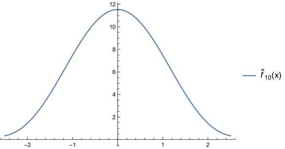
For higher-order moments as represented in (30), we can use Mathematica to perform symbolic high-order differentiation and two dimensional integration. This then gives the higher moments of $\sqrt{n}\theta_{n}$ for all $n$. As all odd moments vanish , we need only focus on the even moments. The numerical results for higher-order moments of $\sqrt{30}\,\theta_{30}$ with $\alpha=0.05$ are summarized in Table 2.

$k$	2	4	6	8	10
$E\left(\sqrt{30}\,\theta_{30}\right)^{k}$	1.038702	3.026394	11.938520	73.447734	545.793589

Table 2: Numerical Results of higher-order moments of $\sqrt{30}\,\theta_{30}$ when $\alpha=0.05$ and the AR(1) processes are assumed independent.

The numerical results of higher-order moments of $\sqrt{30}\,\theta_{30}$ enable us to approximate its density using the Legendre polynomial approximation method (see, for example, [13]). In Figure 1, we present an approximation to the density of $\sqrt{30}\,\theta_{30}$ based on its first ten moments. This approximation shows that the distribution of $\sqrt{30}\,\theta_{30}$ very closely resembles the Gaussian.

Figure 1: The 10th-order polynomial approximation to the probability density function of $\sqrt{30}\,\theta_{30}$ for $\alpha=0.5$. The AR(1) processes are assumed to be independent.

3.4 Correlated increments.

In the previous sections, we have studied the distribution of the scaled empirical correlation of two independent AR(1) processes by deriving formulas for the higher-order moments. The same techniques may also be employed if the AR(1) processes are are now assumed to have correlated increments. Specifically, let us assume that the pairs of the increments $(\xi_{n},\eta_{n})$ are i.i.d. Gaussian random vectors with mean zero and covariance matrix

$$\begin{pmatrix}1&r\\ r&1\end{pmatrix},$$

where $|r|\leq 1$. We then say that these two AR(1) processes are correlated with coefficient $r$. With slight abuse of notation, we also denote by $\theta_{n}$ the empirical correlation of these two correlated AR(1) processes and denote by $\phi_{n}(s_{11},s_{12},s_{22})$ the joint moment generating function. After a similar calculation to that above, we obtain

$$\phi_{n}(s_{11},s_{12},s_{22})=\left(d_{n}(\rho_{r})\,d_{n}(\upsilon_{r})\right)^{-1/2},$$

where $\rho_{r}$ and $\upsilon_{r}$ are defined as

$$\rho_{r}:=\rho_{r}\left(s_{11},s_{12},s_{22}\right)=-\frac{s_{11}+s_{22}+2rs_{12}+\sqrt{(s_{11}-s_{22})^{2}+4(rs_{11}+s_{12})(rs_{22}+s_{12})}}{2},$$

$$\upsilon_{r}:=\upsilon_{r}\left(s_{11},s_{12},s_{22}\right)=-\frac{s_{11}+s_{22}+2rs_{12}-\sqrt{(s_{11}-s_{22})^{2}+4(rs_{11}+s_{12})(rs_{22}+s_{12})}}{2}.$$

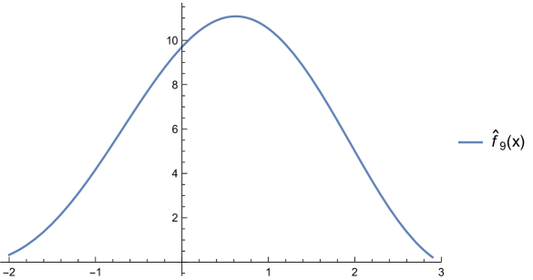
Together with Proposition 4, we can derive expressions for the higher-order moments of $\sqrt{n}\,\theta_{n}$. Furthermore, we can similarly obtain numerical results for the higher-order moments of $\sqrt{n}\,\theta_{n}$ and subsequently approximate its density using Mathematica. The results are summarized in Table 3 and Figure 2. The computation of moments beyond the $9$th order requires substantial memory capacity. Therefore, we only provide numerical results for the moments up to order $9$. Additionally, as demonstrated in Figure 2, using the first $9$ moments is effective in generating a “good” approximation for the density.

$k$	1	2	3	4	5
$E\left(\sqrt{30}\,\theta_{30}\right)^{k}$	0.538403	1.309724	1.697504	4.567613	8.285348
$k$	6	7	8	9
$E\left(\sqrt{30}\,\theta_{30}\right)^{k}$	24.081011	52.901232	165.222506	525.234538

Table 3: Numerical results of higher-order moments of $\sqrt{30}\,\theta_{30}$ for $\alpha=0.05$. The AR(1) processes are assumed to be correlated with $r=0.1$.

Figure 2: The 9th-order polynomial approximation to the probability density function of $\sqrt{30}\,\theta_{30}$ and $\alpha=0.5$. The AR(1) processes are assumed to be correlated with $r=0.1$.

4 Convergence rate of $\sqrt{n}\theta_{n}$.

In this section, we shall investigate the convergence rates of $\sqrt{n}\,\theta_{n}$ to the standard normal distribution. We shall develop upper bounds for the rate of convergence in both Wasserstein distance and in Kolmogorov distance.

We begin by writing $\sqrt{n}\,\theta_{n}$ as

$$\sqrt{n}\,\theta_{n}=\frac{\sqrt{n}\,Z_{12}^{n}}{\sqrt{Z_{11}^{n}Z_{22}^{n}}}$$

We first investigate the convergence rates of the numerator (after scaling) to the standard normal distribution utilizing results of Nourdin and Peccati in (11) and (12). We then study convergence rates for the entire fraction. However, before studying these convergence rates, we first need to prepare several necessary estimates for the eigenvalues of the matrix $K_{n}$ as defined in (14).

4.1 Estimates for eigenvalues of $K_{n}$.

As before, we use $\lambda_{1}\geq\lambda_{2}\geq\dots\geq\lambda_{n}\geq 0$ to denote the eigenvalues of $K_{n}$. In what follows, we will give four lemmas regarding estimates of power sum symmetric polynomials in $\lambda_{1},\lambda_{2},\dots,\lambda_{n}$ and of product of these positive eigenvalues. The first two lemmas, Lemma 6 and 7, involve long but direct calculation. In Lemma 8, we apply Young’s convolution inequality to simplify the calculation. The explicit computation of the product of the positive eigenvalues of $K_{n}$ in Lemma 10 is due to the explicit expression of $d_{n}$. The proofs of the last three lemmas are much more involved and are deferred to Appendix B. We now continue with Lemma 6 below.

Lemma 6.

Let

$$\kappa_{1}(n)=-\frac{\alpha^{2}(1-\alpha^{2n})+(1+\alpha)^{2}}{(1-\alpha^{2})^{2}}+\frac{2\alpha(1+\alpha)(1-\alpha^{n})-\alpha^{2}(1-\alpha^{2n})}{n\,(1-\alpha)^{2}(1-\alpha^{2})}.$$

Then

$$\sum_{k=1}^{n}\lambda_{k}=\frac{1}{1-\alpha^{2}}+\frac{\kappa_{1}(n)}{n}.$$

In particular, for every $n\in\mathds{N}_{+}$,

$$|\kappa_{1}(n)|\leq\frac{\alpha^{2}+(1+\alpha)^{2}}{(1-\alpha^{2})^{2}}+\frac{4|\alpha|+5\alpha^{2}}{(1-\alpha)^{2}(1-\alpha^{2})}=:C_{1}(\alpha).$$

Proof.

We begin by proving the first assertion.

$$\sum_{k=1}^{n}\lambda_{k}=\mathrm{tr}(K_{n})=\sum_{k=1}^{n}\left[\frac{1}{n}\,\frac{1-\alpha^{2k}}{1-\alpha^{2}}-\frac{1}{n^{2}}\,\frac{(1-\alpha^{k})^{2}}{(1-\alpha)^{2}}\right]$$

$$= \frac{1}{n}\,\sum_{k=1}^{n}\frac{1-\alpha^{2k}}{1-\alpha^{2}}-\frac{1}{n^{2}}\,\sum_{k=1}^{n}\frac{1-2\alpha^{k}+\alpha^{2k}}{(1-\alpha)^{2}}$$

$$= \frac{1}{1-\alpha^{2}}-\frac{\alpha^{2}(1-\alpha^{2n})}{n\,(1-\alpha^{2})^{2}}-\frac{1}{n\,(1-\alpha)^{2}}+\frac{2\alpha(1-\alpha^{n})}{n^{2}\,(1-\alpha)^{3}}-\frac{\alpha^{2}(1-\alpha^{2n})}{n^{2}\,(1-\alpha)^{2}(1-\alpha^{2})}$$

$$= \frac{1}{1-\alpha^{2}}-\frac{\alpha^{2}(1-\alpha^{2n})+(1+\alpha)^{2}}{n\,(1-\alpha^{2})^{2}}+\frac{2\alpha(1+\alpha)(1-\alpha^{n})-\alpha^{2}(1-\alpha^{2n})}{n^{2}\,(1-\alpha)^{2}(1-\alpha^{2})}.$$

The second assertion follows immediately by noting that $|\alpha^{2}(1-\alpha^{2n})|\leq\alpha^{2}$ and $|2\alpha(1+\alpha)(1-\alpha^{n})|\leq 4|\alpha|(1+\alpha)$. ∎

We now continue with Lemma 7 below.

Lemma 7.

There exists a bounded function $\kappa_{2}(n)$ on $\mathds{N}_{+}$ such that

$$\sum_{k=1}^{n}\lambda_{k}^{2}=\frac{1+\alpha^{2}}{n\,(1-\alpha^{2})^{3}}+\frac{\kappa_{2}(n)}{n^{2}}.$$

In fact,

$$|\kappa_{2}(n)| \leq \frac{4}{(1-\alpha^{2})^{3}}\,\sup_{n\in\mathds{N}_{+}}n\alpha^{2n+2}+\frac{4\alpha^{2}+\alpha^{4}}{(1-\alpha^{2})^{4}}+\frac{8}{(1-\alpha)^{2}(1-\alpha^{2})}$$

$$+\frac{16|\alpha|}{(1-|\alpha|)(1-\alpha)^{2}(1-\alpha^{2})}+\frac{16}{(1-\alpha)^{4}}=:C_{2}(\alpha).$$

Proof.

See Appendix B. ∎

Lemma 8.

Let

$$C_{3}(\alpha):=\left(\frac{2^{4/3}}{(1-\alpha^{2})^{4/3}(1-|\alpha|^{4/3})}+\frac{16}{(1-\alpha)^{8/3}}\right)^{3}.$$

Then

$$\sum_{k=1}^{n}\lambda_{k}^{4}\leq C_{3}(\alpha)\,n^{-3}.$$

Proof.

See Appendix B. ∎

Remark 9.

It follows directly from Lemma 8 that $\lambda_{k}\leq C_{3}(\alpha)^{1/4}\,n^{-3/4}$ for $k=1,2\dots,n$.

It follows easily from Remark 1 that $\lambda_{1}\geq\lambda_{2}\geq\dots\geq\lambda_{n-1}>0$ but $\lambda_{n}=0$. The following Lemma gives an estimate for the product of $\lambda_{1}$, $\lambda_{2}$, $\dots$, $\lambda_{n-1}$.

Lemma 10.

For $n\geq 2$,

$$\prod_{k=1}^{n-1}\lambda_{k}=n^{-(n-1)}\left(1+\alpha^{2}\frac{n-1}{n}-2\alpha\frac{n-1}{n}\right).$$

Further,

$$(n-1)\sqrt[n-1]{\lambda_{1}\lambda_{2}\dots\lambda_{n-1}}\geq\frac{1}{4}.$$

Proof.

See Appendix B. ∎

4.2 Convergence of $\sqrt{n}Z_{12}^{n}$.

With the above estimates in hand, we are ready to investigate the convergence rate of $\sqrt{n}\theta_{n}$ (after scaling) to the normal distribution. The following theorem reveals the convergence rate of the numerator $\sqrt{n}Z_{12}^{n}$ to the standard normal distribution.

Theorem 11.

Let

$$C_{4}(\alpha):=\frac{(1-\alpha^{2})^{3}}{1+\alpha^{2}}\,\sqrt{\left(C_{2}(\alpha)\right)^{2}+C_{3}(\alpha)}.$$

We have

$$d_{Kol}\left(\sqrt{\frac{(1-\alpha^{2})^{3}}{1+\alpha^{2}}}\sqrt{n}\,Z_{12}^{n},\,\mathcal{N}(0,1)\right)\leq\frac{C_{4}(\alpha)}{\sqrt{n}},$$

$$d_{W}\left(\sqrt{\frac{(1-\alpha^{2})^{3}}{1+\alpha^{2}}}\sqrt{n}\,Z_{12}^{n},\,\mathcal{N}(0,1)\right)\leq\frac{\sqrt{2/\pi}\,C_{4}(\alpha)}{\sqrt{n}}.$$

In particular, $\sqrt{n}Z_{12}^{n}$ converges in distribution to $\mathcal{N}\left(0,\frac{1+\alpha^{2}}{(1-\alpha^{2})^{3}}\right)$ as $n$ tends to $\infty$.

Proof.

Recalling the representation (22) in Section 3.1, we have

$$Z_{12}^{n}=\sum_{k=1}^{n}\lambda_{k}W_{k}V_{k}.$$

There exist orthonormal functions $e_{1},e_{2},\dots,e_{n}$, $f_{1},f_{2},\dots,f_{n}$ on $\mathbb{R}_{+}$ such that

$$Z_{12}^{n}\overset{d}{=}\sum_{k=1}^{n}\lambda_{k}\,\mathcal{I}_{1}(e_{k})\,\mathcal{I}_{1}(f_{k}),$$

where $\mathcal{I}_{1}(h)$ as defined in Section 2 is the first-order Wiener integral of $h$. For simplicity, we use $F_{n}$ to denote $\sum_{k=1}^{n}\lambda_{k}\,\mathcal{I}_{1}(e_{k})\,\mathcal{I}_{1}(f_{k})$. Then, it follows by applying the product formula in (5) that $F_{n}\in\mathcal{H}_{2}$. Note that

$$d_{Kol}\left(\sqrt{\frac{(1-\alpha^{2})^{3}}{1+\alpha^{2}}}\sqrt{n}\,Z_{12}^{n},\,\mathcal{N}(0,1)\right)=d_{Kol}\left(\sqrt{\frac{(1-\alpha^{2})^{3}}{1+\alpha^{2}}}\sqrt{n}\,F_{n},\,\mathcal{N}(0,1)\right),$$

$$d_{W}\left(\sqrt{\frac{(1-\alpha^{2})^{3}}{1+\alpha^{2}}}\sqrt{n}\,Z_{12}^{n},\,\mathcal{N}(0,1)\right)=d_{W}\left(\sqrt{\frac{(1-\alpha^{2})^{3}}{1+\alpha^{2}}}\sqrt{n}\,F_{n},\,\mathcal{N}(0,1)\right).$$

If we can now prove that

$$\sqrt{E\left[\left(1-\frac{1}{2}\left\lVert D\left(\sqrt{\frac{(1-\alpha^{2})^{3}}{1+\alpha^{2}}}\sqrt{n}F_{n}\right)\right\rVert_{\mathcal{H}}^{2}\right)^{2}\right]}$$ (31)

$$= \sqrt{E\left[\left(1-\frac{n(1-\alpha^{2})^{3}}{2(1+\alpha^{2})}\lVert DF_{n}\rVert_{\mathcal{H}}^{2}\right)^{2}\right]}\leq\frac{C_{4}(\alpha)}{\sqrt{n}},$$

then together with the estimates (11) and (12) in Section 2, the desired result will follow. Thus, we proceed to prove (31) below.

By the definition of Malliavin derivative, we have

$$DF_{n}=\sum_{k=1}^{n}\left(\lambda_{k}\,\mathcal{I}_{1}(e_{k})f_{k}+\lambda_{k}\,\mathcal{I}_{1}(f_{k})e_{k}\right).$$

Note that $\langle e_{k},f_{j}\rangle_{\mathcal{H}}=0$ and $\langle e_{k},e_{j}\rangle_{\mathcal{H}}=\langle f_{k},f_{j}\rangle_{\mathcal{H}}=\sigma_{kj}$, where $\sigma_{kj}$ equals $1$ if $k=j$ and $0$ otherwise. It directly follows that

$$\lVert DF_{n}\rVert_{\mathcal{H}}^{2} = \sum_{j,k=1}^{n}\langle\lambda_{k}\,\mathcal{I}_{1}(e_{k})f_{k}+\lambda_{k}\,\mathcal{I}_{1}(f_{k})e_{k},\lambda_{j}\,\mathcal{I}_{1}(e_{j})f_{j}+\lambda_{j}\,\mathcal{I}_{1}(f_{j})e_{j}\rangle_{\mathcal{H}}$$

$$= \sum_{k=1}^{n}\left(\lambda_{k}^{2}\ \mathcal{I}_{1}^{2}(e_{k})+\lambda_{k}^{2}\ \mathcal{I}_{1}^{2}(f_{k})\right).$$

Thus,

$$1-\frac{n(1-\alpha^{2})^{3}}{2(1+\alpha^{2})}\lVert DF_{n}\rVert_{\mathcal{H}}^{2}=1-\frac{n(1-\alpha^{2})^{3}}{2(1+\alpha^{2})}\sum_{k=1}^{n}\left(\lambda_{k}^{2}\ \mathcal{I}_{1}^{2}(e_{k})+\lambda_{k}^{2}\ \mathcal{I}_{1}^{2}(f_{k})\right)$$ (32)

$$= 1-\frac{n(1-\alpha^{2})^{3}}{(1+\alpha^{2})}\sum_{k=1}^{n}\lambda_{k}^{2}-\frac{n(1-\alpha^{2})^{3}}{2(1+\alpha^{2})}\sum_{k=1}^{n}\lambda_{k}^{2}\ \left(\mathcal{I}_{1}^{2}(e_{k})-1\right)$$

$$-\frac{n(1-\alpha^{2})^{3}}{2(1+\alpha^{2})}\sum_{k=1}^{n}\lambda_{k}^{2}\ \left(\mathcal{I}_{1}^{2}(f_{k})-1\right).$$

Noting that $\mathcal{I}(e_{1}),\mathcal{I}(e_{2}),\dots,\mathcal{I}(e_{n})$, $\mathcal{I}(f_{1}),\mathcal{I}(f_{2}),\dots,\mathcal{I}(f_{n})$ are independent standard normal random variables, we have

$$E\left[\mathcal{I}_{1}^{2}(e_{k})-1\right]=E\left[\mathcal{I}_{1}^{2}(f_{k})-1\right]=0,$$

$$E\left[\left(\mathcal{I}_{1}^{2}(e_{k})-1\right)\left(\mathcal{I}_{1}^{2}(f_{k})-1\right)\right]=0,$$

$$E\left[\left(\mathcal{I}_{1}^{2}(e_{k})-1\right)\left(\mathcal{I}_{1}^{2}(e_{j})-1\right)\right]=2\sigma_{kj},$$

$$E\left[\left(\mathcal{I}_{1}^{2}(f_{k})-1\right)\left(\mathcal{I}_{1}^{2}(f_{j})-1\right)\right]=2\sigma_{kj}.$$

Together with (32), routine but lengthy calculation gives that

$$E\left[\left(1-\frac{n(1-\alpha^{2})^{3}}{2(1+\alpha^{2})}\lVert DF_{n}\rVert_{\mathcal{H}}^{2}\right)^{2}\right]$$

$$= \left(1-\frac{n(1-\alpha^{2})^{3}}{(1+\alpha^{2})}\,\sum_{k=1}^{n}\lambda_{k}^{2}\right)^{2}+\frac{n^{2}(1-\alpha^{2})^{6}}{(1+\alpha^{2})^{2}}\,\sum_{k=1}^{n}\lambda_{k}^{4}$$

$$= \left(\frac{\kappa_{2}(n)(1-\alpha^{2})^{3}}{n(1+\alpha^{2})}\right)^{2}+\frac{n^{2}(1-\alpha^{2})^{6}}{(1+\alpha^{2})^{2}}\,\sum_{k=1}^{n}\lambda_{k}^{4}$$

$$\leq \frac{(1-\alpha^{2})^{6}}{(1+\alpha^{2})^{2}}\,\frac{\left(C_{2}(\alpha)\right)^{2}}{n^{2}}+\frac{(1-\alpha^{2})^{6}}{(1+\alpha^{2})^{2}}\,\frac{C_{3}(\alpha)}{n}$$

$$\leq \frac{(1-\alpha^{2})^{6}}{(1+\alpha^{2})^{2}}\,\left(\left(C_{2}(\alpha)\right)^{2}+C_{3}(\alpha)\right)\times n^{-1},$$

where the second equality follows by Lemma 7 and the first inequality follows by Lemma 8 combined with the boundedness of $\kappa_{2}(n)$. Then (31) follows immediately from the last display. ∎

4.3 Convergence in Wasserstein distance.

In this section, we will derive an upper bound for the Wasserstein distance between the distribution of $\sqrt{n}\theta_{n}$ (after scaling) and the standard normal distribution. This result relies on two preparatory lemmas. The first, Lemma 12, proves that the forth moment of $\sqrt{n}Z_{12}^{n}$ is bounded uniformly in $n$. The second, Lemma 13, shows that $Z_{11}^{n}$ and $Z_{22}^{n}$ have inverse second moments uniformly bounded in $n$.

Lemma 12.

Let

$$C_{5}(\alpha):=3^{4}\left(\frac{1+\alpha^{2}}{(1-\alpha^{2})^{3}}+\frac{C_{2}(\alpha)}{10}\right)^{2}.$$

For $n\geq 10$, we have

$$E\left[\left(\sqrt{n}\,Z_{12}^{n}\right)^{4}\right]\leq C_{5}(\alpha).$$

Proof.

Recall that $F_{n}$, as defined in the proof of Theorem 11, has the same distribution as $Z_{12}^{n}$ and belongs to the second Wiener chaos $\mathcal{H}_{2}$. Applying the hypercontractivity property from (6) with $q=2$, $p=2$ and $r=4$, we have

$$\left\{E\left[\left(\sqrt{n}F_{n}\right)^{4}\right]\right\}^{1/4}\leq 3\left\{E\left[\left(\sqrt{n}F_{n}\right)^{2}\right]\right\}^{1/2}.$$

Since $Z_{12}^{n}$ and $F_{n}$ are identically distributed,

$$\left\{E\left[\left(\sqrt{n}Z_{12}^{n}\right)^{4}\right]\right\}^{1/4}\leq 3\left\{E\left[\left(\sqrt{n}Z_{12}^{n}\right)^{2}\right]\right\}^{1/2}.$$ (33)

Note that

$$E\left[\left(\sqrt{n}Z_{12}^{n}\right)^{2}\right]=E\left[n\left(\sum_{k=1}^{n}\lambda_{k}W_{k}V_{k}\right)^{2}\right]=E\left[n\sum_{j,k=1}^{n}\lambda_{k}\lambda_{j}W_{k}V_{k}W_{j}V_{j}\right]$$

$$= n\sum_{k=1}^{n}\lambda_{k}^{2}=\frac{1+\alpha^{2}}{(1-\alpha^{2})^{3}}+\frac{\kappa_{2}(n)}{n}\leq\frac{1+\alpha^{2}}{(1-\alpha^{2})^{3}}+\frac{C_{2}(\alpha)}{10}.$$

Together with (33), the desired result follows. ∎

Lemma 13.

For $n\geq 10$, we have

$$E\left[\left(Z_{11}^{n}\right)^{-2}\right]=E\left[\left(Z_{22}^{n}\right)^{-2}\right]\leq 16\left(2\sqrt{2/\pi}+1\right)^{8}.$$

Proof.

Since $Z_{11}^{n}$ and $Z_{22}^{n}$ are identically distributed, it suffices to prove that $E\left[\left(Z_{11}^{n}\right)^{-2}\right]\leq 16\left(2\sqrt{2/\pi}+1\right)^{8}$. Noting that $\lambda_{n}=0$, we have that

$$Z_{11}^{n}=\sum_{k=1}^{n-1}\lambda_{k}W_{k}^{2}\geq(n-1)\sqrt[n-1]{(\lambda_{1}W_{1}^{2})(\lambda_{2}W_{2}^{2})\dots(\lambda_{n-1}W_{n-1}^{2})}$$

$$= (n-1)\sqrt[n-1]{\lambda_{1}\lambda_{2}\dots\lambda_{n-1}}\,\prod_{k=1}^{n-1}W_{k}^{\frac{2}{n-1}}\geq\frac{1}{4}\,\prod_{k=1}^{n-1}W_{k}^{\frac{2}{n-1}},$$

where the first inequality follows by inequality of arithmetic and geometric means and the second inequality follows by Lemma 10. Invoking the fact that $W_{1},W_{2},\dots,W_{n-1}$ are independent and identically distributed, we have that

$$E\left[\left(Z_{11}^{n}\right)^{-2}\right]\leq 16\,E\left[\prod_{k=1}^{n-1}W_{k}^{-\frac{4}{n-1}}\right]=16\prod_{k=1}^{n-1}E\left[W_{k}^{-\frac{4}{n-1}}\right]=16\,\left\{E\left[W_{1}^{-\frac{4}{n-1}}\right]\right\}^{n-1}.$$

Applying Hölder’s inequality yields

$$E\left[W_{1}^{-\frac{4}{n-1}}\right]\leq\left\{E\left[|W_{1}|^{-\frac{1}{2}}\right]\right\}^{\frac{8}{n-1}}.$$

Thus,

$$E\left[\left(Z_{11}^{n}\right)^{-2}\right]\leq 16\left\{E\left[|W_{1}|^{-\frac{1}{2}}\right]\right\}^{8}.$$

Noting that

$$E\left[|W_{1}|^{-\frac{1}{2}}\right]=2\int_{0}^{\infty}x^{-\frac{1}{2}}\frac{1}{\sqrt{2\pi}}\,e^{-\frac{x^{2}}{2}}\,dx$$

$$= 2\int_{0}^{1}x^{-\frac{1}{2}}\frac{1}{\sqrt{2\pi}}\,e^{-\frac{x^{2}}{2}}\,dx+2\int_{1}^{\infty}x^{-\frac{1}{2}}\frac{1}{\sqrt{2\pi}}\,e^{-\frac{x^{2}}{2}}\,dx$$

$$\leq \sqrt{\frac{2}{\pi}}\int_{0}^{1}x^{-\frac{1}{2}}\,dx+2\int_{1}^{\infty}\frac{1}{\sqrt{2\pi}}\,e^{-\frac{x^{2}}{2}}\,dx$$

$$\leq 2\sqrt{\frac{2}{\pi}}+1,$$

the desired result follows. ∎

With the above preparation in hand, we are ready to derive the upper bound for the Wasserstein distance between the distribution of $\sqrt{n}\theta_{n}$ (after scaling) and the standard normal distribution.

Theorem 14.

For $n\geq 10$, we have

$$d_{W}\left(\sqrt{\frac{1-\alpha^{2}}{1+\alpha^{2}}}\sqrt{n}\theta_{n},\,\mathcal{N}(0,1)\right)\leq\frac{\sqrt{2/\pi}\,C_{4}(\alpha)+C_{6}(\alpha)}{\sqrt{n}},$$

where $C_{4}(\alpha)$ is defined in Theorem 11 and

$$C_{6}(\alpha) := \left(4\left(2\sqrt{2/\pi}+1\right)^{4}\,\sqrt{\frac{1-\alpha^{2}}{1+\alpha^{2}}}+2\left(2\sqrt{2/\pi}+1\right)^{2}\,\frac{1-\alpha^{2}}{\sqrt{1+\alpha^{2}}}\right)\,\left(C_{5}(\alpha)\right)^{\frac{1}{4}}$$

$$\times\left[\frac{2(1+\alpha^{2})}{1-\alpha^{2}}+\frac{(1-\alpha^{2})^{2}\left(C_{1}(\alpha)\right)^{2}}{10}+\frac{(1-\alpha^{2})^{2}C_{2}(\alpha)}{5}\right]^{\frac{1}{2}}.$$

In particular, $\sqrt{n}\theta_{n}$ converges in distribution to $\mathcal{N}\left(0,(1+\alpha^{2})/(1-\alpha^{2})\right)$ as $n\rightarrow\infty$.

Proof.

For simplicity, we use $\sqrt{n}\,\widetilde{\theta}_{n}$ to denote $\sqrt{\frac{(1-\alpha^{2})^{3}}{1+\alpha^{2}}}\sqrt{n}Z_{12}^{n}$. It follows by Lemma 12 that, for $n\geq 10$,

$$E\left[\left(\sqrt{n}\,\widetilde{\theta}_{n}\right)^{4}\right]\leq\frac{(1-\alpha^{2})^{6}}{(1+\alpha^{2})^{2}}\,C_{5}(\alpha).$$ (34)

By Theorem 11 and the triangle inequality, it suffices to prove that

$$d_{W}\left(\sqrt{\frac{1-\alpha^{2}}{1+\alpha^{2}}}\sqrt{n}\theta_{n},\,\sqrt{n}\,\widetilde{\theta}_{n}\right)\leq\frac{C_{6}(\alpha)}{\sqrt{n}}.$$ (35)

Note that

$$d_{W}\left(\sqrt{\frac{1-\alpha^{2}}{1+\alpha^{2}}}\sqrt{n}\theta_{n},\,\sqrt{n}\,\widetilde{\theta}_{n}\right)=\sup_{f\in\mathrm{Lip}(1)}\left|Ef\left(\sqrt{\frac{1-\alpha^{2}}{1+\alpha^{2}}}\sqrt{n}\theta_{n}\right)-Ef\left(\sqrt{n}\,\widetilde{\theta}_{n}\right)\right|.$$

For every $f\in\mathrm{Lip}(1)$, and every pair of integrable random variables $(X,Y)$ on the same probability space, we have that

$$|Ef(X)-Ef(Y)|\leq E|f(X)-f(Y)|\leq E|X-Y|.$$

We now take the supremum over $f\in\mathrm{Lip}(1)$ on both sides of the above display with $X$, $Y$ replaced with $\sqrt{(1-\alpha^{2})/(1+\alpha^{2})}\sqrt{n}\theta_{n}$ and $\sqrt{n}\,\widetilde{\theta}_{n}$, respectively. This yields

$$d_{W}\left(\sqrt{\frac{1-\alpha^{2}}{1+\alpha^{2}}}\sqrt{n}\theta_{n},\,\sqrt{n}\,\widetilde{\theta}_{n}\right)\leq E\left|\sqrt{\frac{1-\alpha^{2}}{1+\alpha^{2}}}\sqrt{n}\theta_{n}-\sqrt{n}\,\widetilde{\theta}_{n}\right|.$$

We now only need to bound the expectation of $|\sqrt{(1-\alpha^{2})/(1+\alpha^{2})}\sqrt{n}\theta_{n}-\sqrt{n}\,\widetilde{\theta}_{n}|$. Note that

$$\sqrt{\frac{1-\alpha^{2}}{1+\alpha^{2}}}\sqrt{n}\theta_{n}-\sqrt{n}\,\widetilde{\theta}_{n}=\frac{\sqrt{n}\,\widetilde{\theta}_{n}}{\sqrt{(1-\alpha^{2})Z_{11}^{n}\times(1-\alpha^{2})Z_{22}^{n}}}-\sqrt{n}\,\widetilde{\theta}_{n}$$

$$= \frac{\sqrt{n}\,\widetilde{\theta}_{n}}{\sqrt{(1-\alpha^{2})Z_{11}^{n}\times(1-\alpha^{2})Z_{22}^{n}}}\,\left(1-\sqrt{(1-\alpha^{2})Z_{11}^{n}\times(1-\alpha^{2})Z_{22}^{n}}\right)$$

$$= \frac{\sqrt{n}\,\widetilde{\theta}_{n}}{\sqrt{(1-\alpha^{2})Z_{11}^{n}\times(1-\alpha^{2})Z_{22}^{n}}}\,\left(1-\sqrt{(1-\alpha^{2})Z_{11}^{n}}\right)$$

$$+\frac{\sqrt{n}\,\widetilde{\theta}_{n}}{\sqrt{(1-\alpha^{2})Z_{11}^{n}\times(1-\alpha^{2})Z_{22}^{n}}}\,\sqrt{(1-\alpha^{2})Z_{11}^{n}}\left(1-\sqrt{(1-\alpha^{2})Z_{22}^{n}}\right)$$

$$= \frac{\sqrt{n}\,\widetilde{\theta}_{n}}{\sqrt{(1-\alpha^{2})Z_{11}^{n}\times(1-\alpha^{2})Z_{22}^{n}}}\,\left(1-\sqrt{(1-\alpha^{2})Z_{11}^{n}}\right)$$

$$+\frac{\sqrt{n}\,\widetilde{\theta}_{n}}{\sqrt{(1-\alpha^{2})Z_{22}^{n}}}\,\left(1-\sqrt{(1-\alpha^{2})Z_{22}^{n}}\right).$$

Then,

$$\left|\sqrt{\frac{1-\alpha^{2}}{1+\alpha^{2}}}\sqrt{n}\theta_{n}-\sqrt{n}\,\widetilde{\theta}_{n}\right|$$ (36)

$$\leq \frac{\left|\sqrt{n}\,\widetilde{\theta}_{n}\right|}{\sqrt{(1-\alpha^{2})Z_{11}^{n}\times(1-\alpha^{2})Z_{22}^{n}}}\,\left|1-\sqrt{(1-\alpha^{2})Z_{11}^{n}}\right|$$

$$+\frac{\left|\sqrt{n}\,\widetilde{\theta}_{n}\right|}{\sqrt{(1-\alpha^{2})Z_{22}^{n}}}\,\left|1-\sqrt{(1-\alpha^{2})Z_{22}^{n}}\right|$$

$$\leq \frac{\left|\sqrt{n}\,\widetilde{\theta}_{n}\right|}{\sqrt{(1-\alpha^{2})Z_{11}^{n}\times(1-\alpha^{2})Z_{22}^{n}}}\,\left|1-(1-\alpha^{2})Z_{11}^{n}\right|$$

$$+\frac{\left|\sqrt{n}\,\widetilde{\theta}_{n}\right|}{\sqrt{(1-\alpha^{2})Z_{22}^{n}}}\,\left|1-(1-\alpha^{2})Z_{22}^{n}\right|,$$

where in the last inequality we have applied the inequality $|1-x|\leq|1-x^{2}|$ for $x\geq 0$. Note that

$$E\left[Z_{11}^{n}\right]=E\left[\sum_{k=1}^{n}\lambda_{k}W_{k}^{2}\right]=\sum_{k=1}^{n}\lambda_{k},$$

and

$$E\left[\left(Z_{11}^{n}\right)^{2}\right]=E\left[\left(\sum_{k=1}^{n}\lambda_{k}W_{k}^{2}\right)^{2}\right]=E\left[\sum_{j,k=1}^{n}\lambda_{k}\lambda_{j}W_{k}^{2}\,W_{j}^{2}\right]$$

$$= \sum_{k=1}^{n}\lambda_{k}^{2}E\left[W_{k}^{4}\right]+\sum_{k\neq j}\lambda_{k}\lambda_{j}E\left[W_{k}^{2}\,W_{j}^{2}\right]=3\sum_{k=1}^{n}\lambda_{k}^{2}+\sum_{k\neq j}\lambda_{k}\lambda_{j}$$

$$= \left(\sum_{k=1}^{n}\lambda_{k}\right)^{2}+2\sum_{k=1}^{n}\lambda_{k}^{2}.$$

Then

$$E\left[\left(1-(1-\alpha^{2})Z_{11}^{n}\right)^{2}\right]$$ (37)

$$= 1-2(1-\alpha^{2})E\left[Z_{11}^{n}\right]+(1-\alpha^{2})^{2}E\left[\left(Z_{11}^{n}\right)^{2}\right]$$

$$= 1-2(1-\alpha^{2})\sum_{k=1}^{n}\lambda_{k}+(1-\alpha^{2})^{2}\left(\sum_{k=1}^{n}\lambda_{k}\right)^{2}+2(1-\alpha^{2})^{2}\sum_{k=1}^{n}\lambda_{k}^{2}$$

$$= \left(1-(1-\alpha^{2})\sum_{k=1}^{n}\lambda_{k}\right)^{2}+2(1-\alpha^{2})^{2}\sum_{k=1}^{n}\lambda_{k}^{2}$$

$$= \frac{(1-\alpha^{2})^{2}(\kappa_{1}(n))^{2}}{n^{2}}+\frac{2(1+\alpha^{2})}{1-\alpha^{2}}\,\frac{1}{n}+\frac{2(1-\alpha^{2})^{2}\kappa_{2}(n)}{n^{2}}$$

$$\leq \left[\frac{2(1+\alpha^{2})}{1-\alpha^{2}}+\frac{(1-\alpha^{2})^{2}\left(C_{1}(\alpha)\right)^{2}}{10}+\frac{(1-\alpha^{2})^{2}C_{2}(\alpha)}{5}\right]\times n^{-1},$$

where in the fourth equality we have invoked Lemma 6 and Lemma 7. Similarly,

$$E\left[\left(1-(1-\alpha^{2})Z_{22}^{n}\right)^{2}\right]\leq\left[\frac{2(1+\alpha^{2})}{1-\alpha^{2}}+\frac{(1-\alpha^{2})^{2}\left(C_{1}(\alpha)\right)^{2}}{10}+\frac{(1-\alpha^{2})^{2}C_{2}(\alpha)}{5}\right]\times n^{-1}.$$

Applying Hölder’s inequality twice yields

$$E\left[\frac{\left|\sqrt{n}\,\widetilde{\theta}_{n}\right|}{\sqrt{(1-\alpha^{2})Z_{11}^{n}\times(1-\alpha^{2})Z_{22}^{n}}}\,\left|1-(1-\alpha^{2})Z_{11}^{n}\right|\right]$$ (38)

$$\leq \left\{E\left[\left(\frac{1}{\sqrt{(1-\alpha^{2})Z_{11}^{n}\times(1-\alpha^{2})Z_{22}^{n}}}\right)^{4}\right]\right\}^{\frac{1}{4}}\,\left\{E\left[\left(\sqrt{n}\,\widetilde{\theta}_{n}\right)\right]^{4}\right\}^{\frac{1}{4}}$$

$$\times\left\{E\left[\left(1-(1-\alpha^{2})Z_{11}^{n}\right)^{2}\right]\right\}^{\frac{1}{2}}$$

$$= \frac{1}{1-\alpha^{2}}\left\{E\left[\left(Z_{11}^{n}\right)^{-2}\right]\right\}^{\frac{1}{4}}\left\{E\left[\left(Z_{22}^{n}\right)^{-2}\right]\right\}^{\frac{1}{4}}\,\left\{E\left[\left(\sqrt{n}\,\widetilde{\theta}_{n}\right)\right]^{4}\right\}^{\frac{1}{4}}$$

$$\times\left\{E\left[\left(1-(1-\alpha^{2})Z_{11}^{n}\right)^{2}\right]\right\}^{\frac{1}{2}}$$

$$\leq 4\left(2\sqrt{2/\pi}+1\right)^{4}\,\sqrt{\frac{1-\alpha^{2}}{1+\alpha^{2}}}\,\left(C_{5}(\alpha)\right)^{\frac{1}{4}}$$

$$\times\left[\frac{2(1+\alpha^{2})}{1-\alpha^{2}}+\frac{(1-\alpha^{2})^{2}\left(C_{1}(\alpha)\right)^{2}}{10}+\frac{(1-\alpha^{2})^{2}C_{2}(\alpha)}{5}\right]^{\frac{1}{2}}\times n^{-\frac{1}{2}},$$

where the first equality follows by noting that $Z_{11}^{n}$ and $Z_{22}^{n}$ are independent and the last inequality follows by combining (34), (37) and Lemma 13. Similarly,

$$E\left[\frac{\left|\sqrt{n}\,\widetilde{\theta}_{n}\right|}{\sqrt{(1-\alpha^{2})Z_{22}^{n}}}\,\left|1-(1-\alpha^{2})Z_{22}^{n}\right|\right]$$ (39)

$$\leq 2\left(2\sqrt{2/\pi}+1\right)^{2}\,\frac{1-\alpha^{2}}{\sqrt{1+\alpha^{2}}}\,\left(C_{5}(\alpha)\right)^{\frac{1}{4}}$$

$$\times\left[\frac{2(1+\alpha^{2})}{1-\alpha^{2}}+\frac{(1-\alpha^{2})^{2}\left(C_{1}(\alpha)\right)^{2}}{10}+\frac{(1-\alpha^{2})^{2}C_{2}(\alpha)}{5}\right]^{\frac{1}{2}}\times n^{-\frac{1}{2}}.$$

Then (35) follows by combining (36), (38) and (39). This completes the proof. ∎

4.4 Convergence in Kolmogorov distance.

In this section, we will derive an upper bound for the Kolmogorov distance between $\sqrt{n}\theta_{n}$ and the standard normal distribution. This result relies on two preparatory lemmas. The first lemma, displayed in Lemma 15 below, is from the work of Michel and Pfanzagl [9]. The lemma provides upper bounds for (i) the Kolmogorov distance between the ratio of two random variables and a standard normal random variable and (ii) the Kolmogorov distance between the sum of two random variables and the standard normal random variable. The second lemma, Lemma 16, provides the asymptotics of $d_{n}\left(t\sqrt{n\ln n}\right)$ and plays an important role in deriving the upper bound.

Lemma 15.

Let $X$, $Y$ and $Z$ be three random variables defined on a probability space $(\Omega,\mathcal{F},P)$ such that $P(Y>0)=1$. Then, for all $\epsilon>0$, we have

1. $d_{Kol}\left(\frac{X}{Y},\,N\right)\leq d_{Kol}(X,N)+P\left(|Y-1|>\epsilon\right)+\epsilon$,

2. $d_{Kol}(X+Z,N)\leq d_{Kol}(X,N)+P\left(|Z|>\epsilon\right)+\epsilon$,

where $N\sim\mathcal{N}(0,1)$.

Proof.

See Michel and Pfanzagl [9]. ∎

Lemma 16.

For every fixed $t\in\mathbb{R}$, as $n$ tends to $\infty$,

$$d_{n}\left(t\sqrt{n\ln n}\right)=(1+o(1))\,e^{-\frac{t}{1-\alpha^{2}}\sqrt{n\ln n}\,-\left[\frac{(1+\alpha^{2})^{2}\,t^{2}}{4(1-\alpha^{2})^{3}}+\frac{t^{2}}{2(1-\alpha^{2})^{2}}-\frac{t^{2}}{4(1-\alpha^{2})}+o(1)\right]\ln n}.$$

Proof.

For simplicity of notation, we use $\gamma_{1,n,\mathrm{ln}}$, $\gamma_{2,n,\mathrm{ln}}$ and $\Delta_{n,\mathrm{ln}}$ to denote $\gamma_{1}\left(t\sqrt{\ln n/n}\right)$, $\gamma_{2}\left(t\sqrt{\ln n/n}\right)$ and $\Delta\left(t\sqrt{\ln n/n}\right)$ respectively. Then, together with Lemma 2, we have

$$d_{n}(t\sqrt{n\ln n})$$ (40)

$$= \frac{\left(\gamma_{1,n,\mathrm{ln}}\right)^{n+1}-\left(\gamma_{2,n,\mathrm{ln}}\right)^{n+1}}{\sqrt{\Delta_{n,\mathrm{ln}}}}-\frac{\alpha^{2}\left[\left(\gamma_{1,n,\mathrm{ln}}\right)^{n}-\left(\gamma_{2,n,\mathrm{ln}}\right)^{n}\right]}{\sqrt{\Delta_{n,\mathrm{ln}}}}$$

$$+\frac{t\sqrt{n\ln n}\left[\left(\gamma_{1,n,\mathrm{ln}}\right)^{n+1}+\left(\gamma_{2,n,\mathrm{ln}}\right)^{n+1}\right]}{n\,\Delta_{n,\mathrm{ln}}}-\frac{(n-1)\alpha^{2}\,t\sqrt{n\ln n}\left[\left(\gamma_{1,n,\mathrm{ln}}\right)^{n}+\left(\gamma_{2,n,\mathrm{ln}}\right)^{n}\right]}{n^{2}\,\Delta_{n,\mathrm{ln}}}$$

$$+\frac{2(n-1)\alpha\,t\sqrt{n\ln n}\left[\left(\gamma_{1,n,\mathrm{ln}}\right)^{n+1}+\left(\gamma_{2,n,\mathrm{ln}}\right)^{n+1}\right]}{n\,\Delta_{n,\mathrm{ln}}\left(n(1-\alpha)^{2}-t\sqrt{n\ln n}\right)}$$

$$-\frac{2(n-2)\alpha^{3}\,t\sqrt{n\ln n}\left[\left(\gamma_{1,n,\mathrm{ln}}\right)^{n}+\left(\gamma_{2,n,\mathrm{ln}}\right)^{n}\right]}{n\,\Delta_{n,\mathrm{ln}}\left(n(1-\alpha)^{2}-t\sqrt{n\ln n}\right)}$$

$$-\frac{2(n+1)\alpha^{2}\,t\sqrt{n\ln n}\left[\left(\gamma_{1,n,\mathrm{ln}}\right)^{n}+\left(\gamma_{2,n,\mathrm{ln}}\right)^{n}\right]}{n\,\Delta_{n,\mathrm{ln}}\left(n(1-\alpha)^{2}-t\sqrt{n\ln n}\right)}+\frac{2\alpha^{4}\,t\sqrt{n\ln n}\left[\left(\gamma_{1,n,\mathrm{ln}}\right)^{n-1}+\left(\gamma_{2,n,\mathrm{ln}}\right)^{n-1}\right]}{\Delta_{n,\mathrm{ln}}\left(n(1-\alpha)^{2}-t\sqrt{n\ln n}\right)}$$

$$+\frac{2\,\alpha^{n+1}(1-\alpha)\,t\sqrt{n\ln n}\left[\gamma_{1,n,\mathrm{ln}}+\gamma_{2,n,\mathrm{ln}}\right]}{n\,\Delta_{n,\mathrm{ln}}\left(n(1-\alpha)^{2}-t\sqrt{n\ln n}\right)}+\frac{4\,\alpha^{n+2}(1-\alpha)\,t\sqrt{n\ln n}}{n\,\Delta_{n,\mathrm{ln}}\left(n(1-\alpha)^{2}-t\sqrt{n\ln n}\right)}.$$

Note that

$$\gamma_{1,n,\mathrm{ln}} = \frac{1-t\sqrt{\frac{\ln n}{n}}+\alpha^{2}+\sqrt{\left(1-t\sqrt{\frac{\ln n}{n}}+\alpha^{2}\right)^{2}-4\alpha^{2}}}{2}$$

$$= \frac{1+\alpha^{2}-t\sqrt{\frac{\ln n}{n}}+(1-\alpha^{2})\sqrt{1-\frac{2(1+\alpha^{2})t}{(1-\alpha^{2})^{2}}\sqrt{\frac{\ln n}{n}}+\frac{t^{2}}{(1-\alpha^{2})^{2}}\frac{\ln n}{n}}}{2}.$$

Applying Taylor’s expansion, it follows after rearrangement that

$$\sqrt{1-\frac{2(1+\alpha^{2})t}{(1-\alpha^{2})^{2}}\sqrt{\frac{\ln n}{n}}+\frac{t^{2}}{(1-\alpha^{2})^{2}}\frac{\ln n}{n}}$$

$$= 1-\frac{(1+\alpha^{2})t}{(1-\alpha^{2})^{2}}\sqrt{\frac{\ln n}{n}}-\left[\frac{(1+\alpha^{2})^{2}t^{2}}{2(1-\alpha^{2})^{4}}-\frac{t^{2}}{2(1-\alpha^{2})^{2}}\right]\frac{\ln n}{n}+o\left(\frac{\ln n}{n}\right).$$

Hence,

$$\gamma_{1,n,\mathrm{ln}}=1-\frac{t}{1-\alpha^{2}}\sqrt{\frac{\ln n}{n}}-\left[\frac{(1+\alpha^{2})^{2}t^{2}}{4(1-\alpha^{2})^{3}}-\frac{t^{2}}{4(1-\alpha^{2})}\right]\frac{\ln n}{n}+o\left(\frac{\ln n}{n}\right).$$

Again, applying Taylor’s expansion, it follows after rearrangement of terms that

$$\ln\left(\gamma_{1,n,\mathrm{ln}}\right)=-\frac{t}{1-\alpha^{2}}\sqrt{\frac{\ln n}{n}}-\left[\frac{(1+\alpha^{2})^{2}t^{2}}{4(1-\alpha^{2})^{3}}+\frac{t^{2}}{2(1-\alpha^{2})^{2}}-\frac{t^{2}}{4(1-\alpha^{2})}\right]\frac{\ln n}{n}+o\left(\frac{\ln n}{n}\right).$$

Then,

$$\left(\gamma_{1,n,\mathrm{ln}}\right)^{n}=\exp\left(n\ln\left(\gamma_{1,n,\mathrm{ln}}\right)\right)=e^{-\frac{t}{1-\alpha^{2}}\sqrt{n\ln n}\,-\left[\frac{(1+\alpha^{2})^{2}\,t^{2}}{4(1-\alpha^{2})^{3}}+\frac{t^{2}}{2(1-\alpha^{2})^{2}}-\frac{t^{2}}{4(1-\alpha^{2})}+o(1)\right]\ln n}.$$

Note that $\gamma_{2,n,\mathrm{ln}}=\alpha^{2}/\gamma_{1,n,\mathrm{ln}}$. Combining this with the fact that $0\leq\alpha^{2}<1$, we have

$$\left(\gamma_{2,n,\mathrm{ln}}\right)^{n}=\alpha^{2n}\left(\gamma_{1,n,\mathrm{ln}}\right)^{-n}$$

$$= e^{n\ln\left(\alpha^{2}\right)+\frac{t}{1-\alpha^{2}}\sqrt{n\ln n}\,+\left[\frac{(1+\alpha^{2})^{2}\,t^{2}}{4(1-\alpha^{2})^{3}}+\frac{t^{2}}{2(1-\alpha^{2})^{2}}-\frac{t^{2}}{4(1-\alpha^{2})}+o(1)\right]\ln n}$$

$$= o(1)\,e^{-\frac{t}{1-\alpha^{2}}\sqrt{n\ln n}\,-\left[\frac{(1+\alpha^{2})^{2}\,t^{2}}{4(1-\alpha^{2})^{3}}+\frac{t^{2}}{2(1-\alpha^{2})^{2}}-\frac{t^{2}}{4(1-\alpha^{2})}+o(1)\right]\ln n}.$$

A routine calculation gives the result that as $n\rightarrow\infty$,

$$\gamma_{1,n,\mathrm{ln}} = 1+o(1),$$

$$\gamma_{2,n,\mathrm{ln}} = \alpha^{2}+o(1),$$

$$\Delta_{n,\mathrm{ln}} = (1-\alpha^{2})^{2}+o(1).$$

Combining the last three displays yields

$$\frac{\left(\gamma_{1,n,\mathrm{ln}}\right)^{n+1}-\left(\gamma_{2,n,\mathrm{ln}}\right)^{n+1}}{\sqrt{\Delta_{n,\mathrm{ln}}}}-\frac{\alpha^{2}\left[\left(\gamma_{1,n,\mathrm{ln}}\right)^{n}-\left(\gamma_{2,n,\mathrm{ln}}\right)^{n}\right]}{\sqrt{\Delta_{n,\mathrm{ln}}}}$$

$$= (1+o(1))\,e^{-\frac{t}{1-\alpha^{2}}\sqrt{n\ln n}\,-\left[\frac{(1+\alpha^{2})^{2}\,t^{2}}{4(1-\alpha^{2})^{3}}+\frac{t^{2}}{2(1-\alpha^{2})^{2}}-\frac{t^{2}}{4(1-\alpha^{2})}+o(1)\right]\ln n}.$$

Then, the desired results follows by noting that the remaining items on the right-hand side of (40) are at most

$$o(1)\,e^{-\frac{t}{1-\alpha^{2}}\sqrt{n\ln n}\,-\left[\frac{(1+\alpha^{2})^{2}\,t^{2}}{4(1-\alpha^{2})^{3}}+\frac{t^{2}}{2(1-\alpha^{2})^{2}}-\frac{t^{2}}{4(1-\alpha^{2})}+o(1)\right]\ln n}.$$

∎

We now turn to the upper bound for the Kolmogorov distance between $\sqrt{n}\theta_{n}$ (after scaling) and standard normal distribution.

Theorem 17.

There exists a constant $C_{7}(\alpha)$ depending on $\alpha$ such that for $n$ sufficiently large,

$$d_{Kol}\left(\sqrt{\frac{1-\alpha^{2}}{1+\alpha^{2}}}\sqrt{n}\theta_{n},\,\mathcal{N}(0,1)\right)\leq C_{7}(\alpha)\,\frac{\sqrt{\ln n}}{\sqrt{n}}.$$

In particular, $\sqrt{n}\theta_{n}$ converges in distribution to $\mathcal{N}\left(0,(1+\alpha^{2})/(1-\alpha^{2})\right)$ as $n\rightarrow\infty$.

Proof.

Let

$$M_{1}:=\frac{1+\alpha^{2}}{1-\alpha^{2}}+1.$$

Note that

$$\sqrt{\frac{1-\alpha^{2}}{1+\alpha^{2}}}\sqrt{n}\theta_{n}=\frac{\sqrt{\frac{(1-\alpha^{2})^{3}}{1+\alpha^{2}}}\sqrt{n}\,Z_{12}^{n}}{\sqrt{(1-\alpha^{2})Z_{11}^{n}\times(1-\alpha^{2})Z_{22}^{n}}}.$$

Invoking Lemma 15 with $X$, $Y$ and $\epsilon$ replaced by $\sqrt{\frac{(1-\alpha^{2})^{3}}{1+\alpha^{2}}}\sqrt{n}\,Z_{12}^{n},$ $\sqrt{(1-\alpha^{2})Z_{11}^{n}\times(1-\alpha^{2})Z_{22}^{n}},$ and $3\,M_{1}\sqrt{\ln n/n}$ respectively, together with Theorem 11, it suffices to prove that

$$P\left(\left|\sqrt{(1-\alpha^{2})Z_{11}^{n}\times(1-\alpha^{2})Z_{22}^{n}}-1\right|>3\,M_{1}\sqrt{\ln n/n}\right)\leq\frac{C_{8}(\alpha)}{\sqrt{n}},$$

for $n$ sufficiently large and for some constant $C_{8}(\alpha)$ depending on $\alpha$.

Applying the inequality $|x-1|\leq|x^{2}-1|$ for $x\geq 0$, we have that

$$\left|\sqrt{(1-\alpha^{2})Z_{11}^{n}\times(1-\alpha^{2})Z_{22}^{n}}-1\right|\leq\left|(1-\alpha^{2})Z_{11}^{n}\times(1-\alpha^{2})Z_{22}^{n}-1\right|$$

$$= \left|\left((1-\alpha^{2})Z_{11}^{n}-1\right)\left((1-\alpha^{2})Z_{22}^{n}-1\right)+\left((1-\alpha^{2})Z_{11}^{n}-1\right)+\left((1-\alpha^{2})Z_{22}^{n}-1\right)\right|$$

$$\leq \left|\left((1-\alpha^{2})Z_{11}^{n}-1\right)\left((1-\alpha^{2})Z_{22}^{n}-1\right)\right|+\left|(1-\alpha^{2})Z_{11}^{n}-1\right|+\left|(1-\alpha^{2})Z_{22}^{n}-1\right|.$$

Then, for $n$ sufficiently large,

$$P\left(\left|\sqrt{(1-\alpha^{2})Z_{11}^{n}\times(1-\alpha^{2})Z_{22}^{n}}-1\right|>3\,M_{1}\sqrt{\ln n/n}\right)$$ (41)

$$\leq P\left(\left|\left((1-\alpha^{2})Z_{11}^{n}-1\right)\left((1-\alpha^{2})Z_{22}^{n}-1\right)\right|>M_{1}\sqrt{\ln n/n}\right)$$

$$+P\left(\left|(1-\alpha^{2})Z_{11}^{n}-1\right|>M_{1}\sqrt{\ln n/n}\right)+P\left(\left|(1-\alpha^{2})Z_{22}^{n}-1\right|>M_{1}\sqrt{\ln n/n}\right)$$

$$\leq P\left(\left|(1-\alpha^{2})Z_{11}^{n}-1\right|>\sqrt{M_{1}\sqrt{\ln n/n}}\right)+P\left(\left|(1-\alpha^{2})Z_{22}^{n}-1\right|>\sqrt{M_{1}\sqrt{\ln n/n}}\right)$$

$$+P\left(\left|(1-\alpha^{2})Z_{11}^{n}-1\right|>M_{1}\sqrt{\ln n/n}\right)+P\left(\left|(1-\alpha^{2})Z_{22}^{n}-1\right|>M_{1}\sqrt{\ln n/n}\right)$$

$$\leq 2P\left(\left|(1-\alpha^{2})Z_{11}^{n}-1\right|>M_{1}\sqrt{\ln n/n}\right)+2P\left(\left|(1-\alpha^{2})Z_{22}^{n}-1\right|>M_{1}\sqrt{\ln n/n}\right)$$

$$= 4P\left(\left|(1-\alpha^{2})Z_{11}^{n}-1\right|>M_{1}\sqrt{\ln n/n}\right),$$

where the last inequality follows by the fact that $M_{1}\sqrt{\ln n/n}<1$ for $n$ sufficiently large and the last equality follows by the identical distribution of $Z_{11}^{n}$ and $Z_{22}^{n}$. Thus, we need only to bound

$$P\left(\left|(1-\alpha^{2})Z_{11}^{n}-1\right|>M_{1}\sqrt{\ln n/n}\right).$$

We first note that

$$P\left(\left|(1-\alpha^{2})Z_{11}^{n}-1\right|>M_{1}\sqrt{\ln n/n}\right)$$ (42)

$$= P\left((1-\alpha^{2})Z_{11}^{n}>1+M_{1}\sqrt{\ln n/n}\right)+P\left(-(1-\alpha^{2})Z_{11}^{n}>-1+M_{1}\sqrt{\ln n/n}\right).$$

Applying Markov’s inequality yields

$$P\left((1-\alpha^{2})Z_{11}^{n}>1+M_{1}\sqrt{\ln n/n}\right)$$ (43)

$$= P\left(\sqrt{n\ln n}(1-\alpha^{2})Z_{11}^{n}>\sqrt{n\ln n}+M_{1}\ln n\right)$$

$$\leq \frac{E\left[e^{\sqrt{n\ln n}(1-\alpha^{2})Z_{11}^{n}}\right]}{e^{\sqrt{n\ln n}+M_{1}\ln n}}.$$

It follows by Remark 9 that

$$\sqrt{n\ln n}(1-\alpha^{2})\,\lambda_{k}\leq C_{3}(\alpha)^{1/4}\,(1-\alpha^{2})\,n^{-1/4}\,\sqrt{\ln n}<1/2$$

for $n$ sufficiently large. Then

$$E\left[e^{\sqrt{n\ln n}(1-\alpha^{2})Z_{11}^{n}}\right]=E\left[e^{\sum_{k}\sqrt{n\ln n}(1-\alpha^{2})\lambda_{k}W_{k}^{2}}\right]=\prod_{k=1}^{n}E\left[e^{\sqrt{n\ln n}(1-\alpha^{2})\lambda_{k}W_{k}^{2}}\right]$$

$$= \prod_{k=1}^{n}\left(1-2\sqrt{n\ln n}\,(1-\alpha^{2})\lambda_{k}\right)^{-\frac{1}{2}}=\left(d_{n}\left(2\sqrt{n\ln n}\,(1-\alpha^{2})\right)\right)^{-\frac{1}{2}}$$

$$= (1+o(1))\,e^{\sqrt{n\ln n}+\left(\frac{1+\alpha^{2}}{1-\alpha^{2}}+o(1)\right)\ln n},$$

where the third equality follows by a standard expression for the mgf of a linear-quadratic functional of a Gaussian random variable, the fourth equality follows by the representation (16) of $d_{n}(\lambda)$, and the last equality follows by invoking Lemma 16 with $t$ replaced by $2(1-\alpha^{2})$. Note that $M_{1}=(1+\alpha^{2})/(1-\alpha^{2})+1$. Together with (43), we have

$$P\left((1-\alpha^{2})Z_{11}^{n}>1+M_{1}\sqrt{\ln n/n}\right)$$

$$\leq (1+o(1))\,e^{\left(\frac{1+\alpha^{2}}{1-\alpha^{2}}+o(1)\right)\ln n-M_{1}\ln n}$$

$$= (1+o(1))\,e^{-(M_{1}-\frac{1+\alpha^{2}}{1-\alpha^{2}}-o(1))\,\ln n}$$

$$= (1+o(1))\,e^{-(1-o(1))\,\ln n}$$

$$\leq \frac{C_{9}(\alpha)}{\sqrt{n}},$$

for $n$ sufficiently large and for some constant $C_{9}(\alpha)$ depending on $\alpha$. Similarly,

$$P\left(-(1-\alpha^{2})Z_{11}^{n}>-1+M_{1}\sqrt{\ln n/n}\right)\leq\frac{C_{10}(\alpha)}{\sqrt{n}},$$

for $n$ large enough for some constant $C_{10}(\alpha)$ depending on $\alpha$. Combining the last two displays with (42) yields that, for $n$ sufficiently large,

$$P\left(\left|(1-\alpha^{2})Z_{11}^{n}-1\right|>M_{1}\sqrt{\ln n/n}\right)\leq\frac{C_{9}(\alpha)+C_{10}(\alpha)}{\sqrt{n}}.$$

The desired result then follows by combining the last display and (41). ∎

Remark 18.

On a practical level, the study of the aforementioned convergence rates should be of direct use to practitioner wishing to conduct tests of independence between two AR(1) processes with smaller sample sizes. For example, suppose that a practitioner studying time series data that can be appropriately modeled as AR(1) processes is considering employing the $n^{-1/2}$ rate of convergence in Wasserstein distance as mentioned above. This rate would lead the practitioner to conclude that in order to achieve an error of 1% between the empirical correlation and the standard Gaussian, one would need 10,000 data points. Furthermore, this informs the practitioner that, should the sample size of these two processes be considerably less than 10,000, that the exact distribution of the scaled empirical correlation (rather than its scaled asymptotic distribution) should be utilized.

5 Power for a test of independence.

The purpose of this section is to study a test of independence between two AR(1) processes with Gaussian increments using their path data. For the two AR(1) processes defined in (3), we propose the null hypothesis as

$$H_{0}:\{X_{n}\}_{n=0}^{\infty}\text{ and }\{Y_{n}\}_{n=0}^{\infty}\text{ are independent},$$

and the alternative hypothesis as

$$H_{a}:\{X_{n}\}_{n=0}^{\infty}\text{ and }\{Y_{n}\}_{n=0}^{\infty}\text{ are correlated with coefficient $r$}.$$

We pause to provide some further explanation for the two hypotheses mentioned above. For the null hypothesis, we define independence between $\{X_{n}\}_{n=0}^{\infty}$ and $\{Y_{n}\}_{n=0}^{\infty}$ as the increments $\xi_{1},\xi_{2},\xi_{3},\dots,\eta_{1},\eta_{2},\eta_{3},\dots$ being independent. In contrast, for the alternative hypothesis, we say that $\{X_{n}\}_{n=0}^{\infty}$ and $\{Y_{n}\}_{n=0}^{\infty}$ are correlated with coefficient $r$ if the pairs of increments $(\xi_{n},\eta_{n})$ are i.i.d. Gaussian random vectors with mean zero and covariance matrix

$$\begin{pmatrix}1&r\\ r&1\end{pmatrix},$$

where $|r|\leq 1$ and $r\neq 0$.

The asymptotic normality of $\sqrt{n}\,\theta_{n}$, as presented in Section 4, indicates that, under the null hypothesis $H_{0}$, the rejection region shall be

$$|\sqrt{n}\,\theta_{n}|>c_{a},$$

where $c_{a}>0$ is selected according to the given level of the test. In this section, we will study the power of the above statistical test. We will provide a lower bound for the power and prove that it converges to $1$ as $n$ tends to $\infty$. The key ingredient for doing so shall be the convergence rate of the distribution of $\sqrt{n}\,(\theta_{n}-r)$ to the normal distribution under the alternative hypothesis, the latter to be exposed in Section 5.1. Relying on the convergence rate, we study the power of the test in Section 5.2.

5.1 Convergence rate under $H_{a}$.

In this section, we will study the Kolmogorov distance between $\sqrt{n}\,(\theta_{n}-r)$ and the standard normal distribution under the alternative hypothesis. Therefore, in the remainder of this section, we shall assume that the pairs of random variables $(\xi_{n},\eta_{n})$ are i.i.d. Gaussian vectors with mean zero and covariance matrix

$$\begin{pmatrix}1&r\\ r&1\end{pmatrix}.$$

For purposes of simplicity, we will continue to use the notation given in Section 2 and Section 3.1. That is,

$$\theta_{n}=\frac{Z_{12}^{n}}{\sqrt{Z_{11}^{n}Z_{22}^{n}}},$$

and $Z_{11}^{n}$, $Z_{12}^{n}$, and $Z_{22}^{n}$ can be simplified as

$$Z_{11}^{n}=\sum_{k=1}^{n}\lambda_{k}\,W_{k}^{2},\ Z_{12}^{n}=\sum_{k=1}^{n}\lambda_{k}\,W_{k}V_{k},\ \text{and }Z_{22}^{n}=\sum_{k=1}^{n}\lambda_{k}\,V_{k}^{2},$$

where

$$\left(W_{1},W_{2},\dots,W_{n}\right)^{\intercal}:=P_{n}\,\mathbf{\Xi}_{n}=P_{n}\,\left(\xi_{1},\xi_{2},\dots,\xi_{n}\right)^{\intercal}$$

$$\left(V_{1},V_{2},\dots,V_{n}\right)^{\intercal}:=P_{n}\,\mathbf{H}_{n}=P_{n}\left(\eta_{1},\eta_{2},\dots,\eta_{n}\right)^{\intercal}.$$

As defined in Section 3.1, $P_{n}$ is an orthogonal matrix. By the invariance of distribution of Gaussian random vector under orthogonal transformation, it may be easily shown that the pairs of random variables $(W_{n},V_{n})$ are still i.i.d. Gaussian vectors with mean zero and covariance matrix

$$\begin{pmatrix}1&r\\ r&1\end{pmatrix}.$$

Then

$$\theta_{n}-r=\frac{Z_{12}^{n}}{\sqrt{Z_{11}^{n}Z_{22}^{n}}}-r=\frac{Z_{12}^{n}-r\sqrt{Z_{11}^{n}Z_{22}^{n}}}{\sqrt{Z_{11}^{n}Z_{22}^{n}}}=\frac{\left(Z_{12}^{n}\right)^{2}-r^{2}\,Z_{11}^{n}Z_{22}^{n}}{\sqrt{Z_{11}^{n}Z_{22}^{n}}\left(Z_{12}^{n}+r\sqrt{Z_{11}^{n}Z_{22}^{n}}\right)}.$$

In what follows, we will first investigate the asymptotics of the scaled numerator of $\theta_{n}-r$, i.e., $\sqrt{n}\,\left(\left(Z_{11}^{n}\right)^{2}-r^{2}\,Z_{11}^{n}Z_{22}^{n}\right)$. We then study the tail of the denominator of $\theta_{n}-r$. Finally, we will derive the asymptotics of $\theta_{n}-r$ by invoking Lemma 15. These results are encapsulated in Theorem 19, Theorem 20 and Theorem 21.

Theorem 19.

Let

$$C_{11}(\alpha,r) := C_{19}(\alpha,r)+\frac{1+8r^{2}+4r^{4}}{r^{2}}\,\frac{(1-\alpha^{2})^{5}}{1+\alpha^{2}}\,C_{3}(\alpha)+1$$

$$+\,\frac{1+2r^{2}}{2|r|}\sqrt{\frac{(1-\alpha^{2})^{5}}{1+\alpha^{2}}}\left(\frac{1+\alpha^{2}}{(1-\alpha^{2})^{3}}+C_{2}(\alpha)\right),$$

with $C_{19}(\alpha,r)$ defined in Theorem 30. Under the alternative hypothesis $H_{a}$, we have

$$d_{Kol}\left(\frac{1}{2r(1-r^{2})}\sqrt{\frac{(1-\alpha^{2})^{5}}{1+\alpha^{2}}}\,\sqrt{n}\left(\left(Z_{11}^{n}\right)^{2}-r^{2}\,Z_{11}^{n}Z_{22}^{n}\right),\,\mathcal{N}(0,1)\right)\leq\frac{C_{11}(\alpha,r)}{\sqrt{n}}.$$

Proof.

See Appendix C. ∎

Note that $M_{1}=\frac{1+\alpha^{2}}{1-\alpha^{2}}+1$, as was defined in the proof of Theorem 17. We also define

$$M_{2}:=\frac{1+r^{2}}{2r^{2}}\,\frac{1+\alpha^{2}}{1-\alpha^{2}}+1.$$

We now continue with Theorem 20 below.

Theorem 20.

Under the alternative hypothesis $H_{a}$, there exists a constant $C_{12}(\alpha,r)$ such that for $n$ sufficiently large,

$$P\left(\left|\frac{Z_{12}^{n}\sqrt{Z_{11}^{n}Z_{22}^{n}}+rZ_{11}^{n}Z_{22}^{n}}{2r/(1-\alpha^{2})^{2}}-1\right|>\frac{1}{2}(6M_{1}+M_{2}+3M_{1}M_{2})\sqrt{\frac{\ln n}{n}}\right)\leq\frac{C_{12}(\alpha,r)}{\sqrt{n}}.$$

Proof.

See Appendix C. ∎

With the above two Theorems, we arrive at our main theorem in this section.

Theorem 21.

Under the alternative hypothesis $H_{a}$, there exists a constant $C_{13}(\alpha,r)$ such that for $n$ large enough,

$$d_{Kol}\left(\frac{1}{1-r^{2}}\sqrt{\frac{1-\alpha^{2}}{1+\alpha^{2}}}\sqrt{n}(\theta_{n}-r),\,\mathcal{N}(0,1)\right)\leq C_{13}(\alpha,r)\times\sqrt{\frac{\ln n}{n}}.$$

Proof.

Note that

$$\frac{1}{1-r^{2}}\sqrt{\frac{1-\alpha^{2}}{1+\alpha^{2}}}\sqrt{n}(\theta_{n}-r)=\frac{\frac{1}{2r(1-r^{2})}\sqrt{\frac{(1-\alpha^{2})^{5}}{1+\alpha^{2}}}\,\sqrt{n}\left(\left(Z_{11}^{n}\right)^{2}-r^{2}\,Z_{11}^{n}Z_{22}^{n}\right)}{\frac{Z_{12}^{n}\sqrt{Z_{11}^{n}Z_{22}^{n}}+rZ_{11}^{n}Z_{22}^{n}}{2r/(1-\alpha^{2})^{2}}}.$$

Together with Theorem 19 and Theorem 20, the desired result follows immediately by invoking Lemma 15 with

$$X=\frac{1}{2r(1-r^{2})}\sqrt{\frac{(1-\alpha^{2})^{5}}{1+\alpha^{2}}}\,\sqrt{n}\left(\left(Z_{11}^{n}\right)^{2}-r^{2}\,Z_{11}^{n}Z_{22}^{n}\right),$$

$$Y=\frac{Z_{12}^{n}\sqrt{Z_{11}^{n}Z_{22}^{n}}+rZ_{11}^{n}Z_{22}^{n}}{2r/(1-\alpha^{2})^{2}},$$

$$\epsilon=\frac{1}{2}(6M_{1}+M_{2}+3M_{1}M_{2})\sqrt{\frac{\ln n}{n}}.$$

∎

5.2 Power.

In Section 5.1, we derived the rate of convergence of $\theta_{n}-r$ (after scaling) to the normal distribution under the alternative hypothesis $H_{a}$. We now proceed to study the power of the test with rejection region

$$|\sqrt{n}\,\theta_{n}|>c_{a}.$$

We first recall a trivial property of the Kolmogorov distance. For a pair of random variables $(X,Y)$, we have that for any constant $c$,

$$\left|P\left(X>c\right)-P\left(Y>c\right)\right|\leq d_{Kol}(X,Y),$$

$$\left|P\left(X<c\right)-P\left(Y<c\right)\right|\leq d_{Kol}(X,Y).$$

Indeed, by the definition of Kolmogorov distance,

$$\left|P\left(X>c\right)-P\left(Y>c\right)\right|=\left|\left(1-P(X\leq c)\right)-\left(1-P(Y\leq c)\right)\right|$$

$$= \left|P(X\leq c)-P(Y\leq c)\right|\leq d_{Kol}(X,Y).$$

Further,

$$\left|P\left(X<c\right)-P\left(Y<c\right)\right|=\left|\lim_{k\rightarrow\infty}\left(P\left(X<c-1/k\right)-P\left(Y<c-1/k\right)\right)\right|\leq d_{Kol}(X,Y).$$

We now turn to the power of the test. Let $\Phi(x)$ be the tail of the standard normal distribution, i.e.,

$$\Phi(x)=\int_{x}^{\infty}\,\frac{1}{\sqrt{2\pi}}\,e^{-\frac{y^{2}}{2}}\,dy.$$

Under the alternative hypothesis $H_{a}$, the power is

$$P\left(|\sqrt{n}\,\theta_{n}|>c_{a}\Big{|}H_{a}\right)=P\left(\sqrt{n}\,\theta_{n}>c_{a}\Big{|}H_{a}\right)+P\left(\sqrt{n}\,\theta_{n}<-c_{a}\Big{|}H_{a}\right).$$

Applying Theorem 21 and the aforementioned property of the Kolmogorov distance, we have for $n$ sufficiently large,

$$P\left(\sqrt{n}\,\theta_{n}>c_{a}\Big{|}H_{a}\right)=P\left(\frac{1}{1-r^{2}}\sqrt{\frac{1-\alpha^{2}}{1+\alpha^{2}}}\sqrt{n}\left(\theta_{n}-r\right)>\frac{1}{1-r^{2}}\sqrt{\frac{1-\alpha^{2}}{1+\alpha^{2}}}\left(c_{a}-\sqrt{n}r\right)\right)$$

$$\geq \Phi\left(\frac{1}{1-r^{2}}\sqrt{\frac{1-\alpha^{2}}{1+\alpha^{2}}}\left(c_{a}-\sqrt{n}r\right)\right)-C_{13}(\alpha,r)\sqrt{\frac{\ln n}{n}}$$

Similarly,

$$P\left(\sqrt{n}\,\theta_{n}<-c_{a}\Big{|}H_{a}\right)\geq\Phi\left(\frac{1}{1-r^{2}}\sqrt{\frac{1-\alpha^{2}}{1+\alpha^{2}}}\left(c_{a}+\sqrt{n}r\right)\right)-C_{13}(\alpha,r)\sqrt{\frac{\ln n}{n}}.$$

Combining last three displays yields

$$P\left(|\sqrt{n}\,\theta_{n}|>c_{a}\Big{|}H_{a}\right) \geq \Phi\left(\frac{1}{1-r^{2}}\sqrt{\frac{1-\alpha^{2}}{1+\alpha^{2}}}\left(c_{a}-\sqrt{n}r\right)\right)$$ (44)

$$+\,\Phi\left(\frac{1}{1-r^{2}}\sqrt{\frac{1-\alpha^{2}}{1+\alpha^{2}}}\left(c_{a}+\sqrt{n}r\right)\right)-2C_{13}(\alpha,r)\sqrt{\frac{\ln n}{n}}.$$

In the case $r\neq 0$, we can see easily, the right-hand side of (44) tends to $1$ as $n$ tends to $\infty$. We therefore include that our test with rejection region is $|\sqrt{n}\,\theta_{n}|>c_{a}$ has asymptotic power tending towards 1.

6 Second Wiener chaos innovations.

As mentioned in the introduction, we will now study the asymptotics of the empirical correlation for two independent AR(1) processes with second Wiener chaos innovations. The two AR(1) processes are formulated as follows:

$$\begin{cases}X_{n}=\alpha X_{n-1}+\xi_{n},\quad n\in\mathds{N}_{+}\\ \xi_{n}=\sum_{\delta=1}^{\infty}\sigma_{\delta}(S_{n,\delta}^{2}-1)\\ X_{0}=0\end{cases}\text{ and }\begin{cases}Y_{n}=\beta Y_{n-1}+\eta_{n},\quad n\in\mathds{N}_{+}\\ \eta_{n}=\sum_{\delta=1}^{\infty}\tau_{\delta}(T_{n,\delta}^{2}-1)\\ Y_{0}=0\end{cases}$$ (45)

where $\alpha$ and $\beta$ are real numbers where both $|\alpha|<1$ and $|\beta|<1$. Furthermore, $\{\xi_{n}\}_{n=1}^{\infty}$ and $\{\eta_{n}\}_{n=1}^{\infty}$ are two independent i.i.d. sequences of increments in the second Wiener chaos. It turns out these two sequences can be expressed in the forms shown in the second line of (45), where $\{S_{n,\delta},\,n\geq 1,\delta\geq 1\}$ and $\{T_{n,\delta},\,n\geq 1,\delta\geq 1\}$ are two families of i.i.d. standard Gaussian random variables defined on a Wiener space $(\Omega,\mathcal{F},P)$, and $\{\sigma_{\delta},\,\delta\geq 1\}$ and $\{\tau_{\delta},\,\delta\geq 1\}$ are two sequences of real numbers satisfying

$$\sum_{\delta=1}^{\infty}\sigma_{\delta}^{2}<\infty\quad\text{ and }\quad\sum_{\delta=1}^{\infty}\tau_{\delta}^{2}<\infty.$$ (46)

For more details, we refer the reader to [11, Section 2.7.4]. We shall later see that, when considering asymptotic analysis, that we may relax the restrictions posed on these two AR(1) processes by allowing them to have distinct parameters and different distributions of increments.

We continue with the model given in (45). A routine calculation gives that $\{X_{n},\,n\geq 1\}$ and $\{Y_{n},\,n\geq 1\}$ can be expressed as

$$X_{i} =\sum_{k=1}^{i}\alpha^{i-k}\sum_{\delta=1}^{\infty}\sigma_{\delta}(S_{k,\delta}^{2}-1),$$

$$Y_{i} =\sum_{k=1}^{i}\beta^{i-k}\sum_{\delta=1}^{\infty}\tau_{\delta}(T_{k,\delta}^{2}-1).$$

Again, as before, we define the empirical variances and covariance as follows:

$$Z_{11}^{n} := \frac{1}{n}\sum_{i=1}^{n}X_{i}^{2}-\frac{1}{n^{2}}\left(\sum_{i=1}^{n}X_{i}\right)^{2},$$ (47)

$$Z_{22}^{n} := \frac{1}{n}\sum_{i=1}^{n}Y_{i}^{2}-\frac{1}{n^{2}}\left(\sum_{i=1}^{n}Y_{i}\right)^{2},$$ (48)

$$Z_{12}^{n} := \frac{1}{n}\sum_{i=1}^{n}X_{i}Y_{i}-\frac{1}{n^{2}}\left(\sum_{i=1}^{n}X_{i}\right)\left(\sum_{i=1}^{n}Y_{i}\right),$$ (49)

where the empirical correlation remains defined as

$$\theta_{n}:=\frac{Z_{12}^{n}}{\sqrt{Z_{11}^{n}Z_{22}^{n}}}.$$ (50)

The main objective of this section is to study the asymptotic distribution of the empirical correlation and to provide its rate of convergence rate in Kolmogorov distance to the standard normal. These objectives are summarized in Theorem 22 below.

Theorem 22.

Under condition (46), with the empirical correlation $\theta_{n}$ defined in (50), there exists a constant $C_{24}(\alpha,\beta)$ only depending on $\alpha$ and $\beta$ such that for $n\geq 3$,

$$d_{Kol}\left(\sqrt{\frac{1-\alpha\beta}{1+\alpha\beta}}\,\sqrt{n}\theta_{n},\,\mathcal{N}(0,1)\right)\leq C_{24}(\alpha,\beta)\times\sqrt{\frac{\ln n}{n}},$$

In particular, $\sqrt{n}\theta_{n}$ is asymptotically normal, namely

$$\sqrt{n}\theta_{n}\overset{D}{\longrightarrow}\mathcal{N}\left(0,\frac{1+\alpha\beta}{1-\alpha\beta}\right).$$

The proof of Theorem 22 follows a similar approach to the proofs of Theorem 17 and Theorem 21. Indeed, the most challenging mathematical task lies in deriving the convergence rate, which is broken down into three distinct steps. In the first step, we represent the numerator of the empirical correlation, $Z_{12}^{n}$, as a quadruple Wiener integral, specifically within the fourth Wiener chaos. This representation enables us to derive the convergence rate of $Z_{12}^{n}$ (after scaling) to the standard normal distribution in Kolmogorov distance (using (8)). We then establish a sharp concentration inequality for the denominator of the empirical correlation. Finally, we utilize Lemma 15 to transform the convergence rate of the scaled numerator into the convergence rate of the entire scaled fraction. The details are presented in Appendix D.

7 Appendix A

The alternative characteristic polynomial $d_{n}(\lambda)$ plays a key role in calculating the joint moment generating function $\phi_{n}(s_{11},s_{12},s_{22})$ (Theorem 3). An explicit formula for $d_{n}(\lambda)$ is given in Lemma 2. The purpose of this appendix is to prove Lemma 2.

7.1 Proof of Lemma 2

For simplicity, we will start with $d_{n}(n^{2}\lambda)$. By the definition of $d_{n}(\lambda)$, we have

$$d_{n}(n^{2}\lambda)=\det(I_{n}-n^{2}\lambda K_{n})=\det\left(I_{n}-\left\{n\lambda\,\frac{\alpha^{|k-j|}-\alpha^{k+j}}{1-\alpha^{2}}-\lambda\,\frac{(1-\alpha^{k})(1-\alpha^{j})}{(1-\alpha)^{2}}\right\}_{j,k=1}^{n}\right).$$

Let $A_{n}$ denote the $n\times n$ matrix

$$I_{n}-\left\{n\lambda\,\frac{\alpha^{|k-j|}-\alpha^{k+j}}{1-\alpha^{2}}\right\}_{j,k=1}^{n},$$

and let $B_{n}$ denote the $n\times n$ matrix

$$\left\{\lambda\,\frac{(1-\alpha^{k})(1-\alpha^{j})}{(1-\alpha)^{2}}\right\}_{j,k=1}^{n}.$$

Then $d_{n}(n^{2}\lambda)=\det(A_{n}+B_{n})$.

We now perform elementary column operations and then perform elementary row operations to $A_{n}$ and $B_{n}$ simultaneously. We do so by first adding $(-\alpha)\times$ the $(j-1)$-th column of $A_{n}$ to its $j$-th column in the order $j=n,n-1,\dots,2$. We then obtain

$$\bar{A}_{n}:=\left(\begin{matrix}1-n\lambda&-\alpha&0&\cdots&0&0\\ -n\lambda\alpha&1-n\lambda&-\alpha&\cdots&0&0\\ -n\lambda\alpha^{2}&-n\lambda\alpha&1-n\lambda&\cdots&0&0\\ \vdots&\vdots&\vdots&\ddots&\vdots&\vdots\\ -n\lambda\alpha^{n-2}&-n\lambda\alpha^{n-3}&-n\lambda\alpha^{n-4}&\cdots&1-n\lambda&-\alpha\\ -n\lambda\alpha^{n-1}&-n\lambda\alpha^{n-2}&-n\lambda\alpha^{n-3}&\cdots&-n\lambda\alpha&1-n\lambda\end{matrix}\right).$$

Performing the same column operations on $B_{n}$, we obtain

$$\bar{B}_{n}:=\left(\begin{matrix}\lambda\frac{1-\alpha}{1-\alpha}&\lambda\frac{1-\alpha}{1-\alpha}&\lambda\frac{1-\alpha}{1-\alpha}&\cdots&\lambda\frac{1-\alpha}{1-\alpha}\vspace{1ex}\\ \lambda\frac{1-\alpha^{2}}{1-\alpha}&\lambda\frac{1-\alpha^{2}}{1-\alpha}&\lambda\frac{1-\alpha^{2}}{1-\alpha}&\cdots&\lambda\frac{1-\alpha^{2}}{1-\alpha}\vspace{1ex}\\ \lambda\frac{1-\alpha^{3}}{1-\alpha}&\lambda\frac{1-\alpha^{3}}{1-\alpha}&\lambda\frac{1-\alpha^{3}}{1-\alpha}&\cdots&\lambda\frac{1-\alpha^{3}}{1-\alpha}\\ \vdots&\vdots&\vdots&\ddots&\vdots\\ \lambda\frac{1-\alpha^{n}}{1-\alpha}&\lambda\frac{1-\alpha^{n}}{1-\alpha}&\lambda\frac{1-\alpha^{n}}{1-\alpha}&\cdots&\lambda\frac{1-\alpha^{n}}{1-\alpha}\\ \end{matrix}\right).$$

Since the determinant is invariant by adding one column multiplied by a scalar to another column, we have that $\det(A_{n}+B_{n})=\det(\bar{A}_{n}+\bar{B}_{n})$. We then add $(-\alpha)\times$ the $(j-1)$-th row of $\bar{A}_{n}$ to its $j$-th row in the order $j=n,n-1,\dots,2$ and obtain a tri-diagonal matrix

$$\widetilde{A}_{n}:=\left(\begin{matrix}1-n\lambda&-\alpha&0&\cdots&0&0\\ -\alpha&1-n\lambda+\alpha^{2}&-\alpha&\cdots&0&0\\ 0&-\alpha&1-n\lambda+\alpha^{2}&\cdots&0&0\\ \vdots&\vdots&\vdots&\ddots&\vdots&\vdots\\ 0&0&0&\cdots&1-n\lambda+\alpha^{2}&-\alpha\\ 0&0&0&\cdots&-\alpha&1-n\lambda+\alpha^{2}\end{matrix}\right).$$

We make the same row operations to $\bar{B}_{n}$ and obtain

$$\widetilde{B}_{n}:=\lambda\,b_{n}b_{n}^{\intercal},$$

where $b_{n}:=(1,1,\dots,1)^{\intercal}$ is a $n\times 1$ column vector. Again, since the determinant is invariant to the addition of one row multiplied by a scalar to another row, we have $\det(\bar{A}_{n}+\bar{B}_{n})=\det(\widetilde{A}_{n}+\widetilde{B}_{n})=\det(\widetilde{A}_{n}+\lambda\,b_{n}b_{n}^{\intercal})$. Hence,

$$d_{n}(n^{2}\lambda)=\det(\widetilde{A}_{n}+\lambda\,b_{n}b_{n}^{\intercal}).$$ (51)

Before proceeding to calculate $d_{n}(n^{2}\lambda)$, we pause here to introduce two new determinants, closely related to $d_{n}(n^{2}\lambda)$. For $n\in\mathds{N}_{+}$, let us denote by $p_{n}(\lambda)$ the following $n\times n$ determinant

$$\left|\begin{matrix}1-\lambda+\alpha^{2}&-\alpha&0&\cdots&0&0\\ -\alpha&1-\lambda+\alpha^{2}&-\alpha&\cdots&0&0\\ 0&-\alpha&1-\lambda+\alpha^{2}&\cdots&0&0\\ \vdots&\vdots&\vdots&\ddots&\vdots&\vdots\\ 0&0&0&\cdots&1-\lambda+\alpha^{2}&-\alpha\\ 0&0&0&\cdots&-\alpha&1-\lambda+\alpha^{2}\end{matrix}\right|.$$ (52)

Let us denote by $q_{n}(\lambda)$ the following $n\times n$ determinant

$$\left|\begin{matrix}1-\lambda&-\alpha&0&\cdots&0&0\\ -\alpha&1-\lambda+\alpha^{2}&-\alpha&\cdots&0&0\\ 0&-\alpha&1-\lambda+\alpha^{2}&\cdots&0&0\\ \vdots&\vdots&\vdots&\ddots&\vdots&\vdots\\ 0&0&0&\cdots&1-\lambda+\alpha^{2}&-\alpha\\ 0&0&0&\cdots&-\alpha&1-\lambda+\alpha^{2}\end{matrix}\right|.$$

By convention, $p_{0}(\lambda)=q_{0}(\lambda)=1$. It follows immediately that, for $n\in\mathds{N}_{+}$, $q_{n}(\lambda)=p_{n}(\lambda)-\alpha^{2}\,p_{n-1}(\lambda)$. To make sure this equation also holds for $n=0$, we let $p_{-1}(\lambda)=0$. Further, expanding determinant (52) by its first row, we have that for $n\geq 3$,

$$p_{n}(\lambda)=(1-\lambda+\alpha^{2})\,p_{n-1}(\lambda)-\alpha^{2}\,p_{n-2}(\lambda).$$

We can easily check that the above iterative formula for $p_{n}(\lambda)$ also holds for $n=1,2$. Further, this iterative formula tells us that for $\lambda\neq(1+\alpha)^{2}$ or $(1-\alpha)^{2}$, $p_{n}(\lambda)$ must have the form

$$C_{1}\,\gamma_{1}^{n}+C_{2}\,\gamma_{2}^{n},$$

where

$$\gamma_{1}=\gamma_{1}(\lambda)=\frac{(1-\lambda+\alpha^{2})+\sqrt{(1-\lambda+\alpha^{2})^{2}-4\alpha^{2}}}{2},$$

$$\gamma_{2}=\gamma_{2}(\lambda)=\frac{(1-\lambda+\alpha^{2})-\sqrt{(1-\lambda+\alpha^{2})^{2}-4\alpha^{2}}}{2},$$

and $C_{1}$, $C_{2}$ are two constants. Note that as defined in (27),

$$\Delta=\Delta(\lambda)=(1-\lambda+\alpha^{2})^{2}-4\alpha^{2}.$$

Since $p_{1}(\lambda)=1-\lambda+\alpha^{2}$ and $p_{2}(\lambda)=(1-\lambda+\alpha^{2})^{2}-\alpha^{2}$, the constants $C_{1}$ and $C_{2}$ can be determined as

$$C_{1}=\frac{\gamma_{1}}{\sqrt{\Delta}}\quad\text{and}\quad C_{2}=-\frac{\gamma_{2}}{\sqrt{\Delta}}.$$

Hence, for $n\geq-1$ and $\lambda\neq(1+\alpha)^{2}$ or $(1-\alpha)^{2}$,

$$p_{n}(\lambda) = \frac{\gamma_{1}^{n+1}-\gamma_{2}^{n+1}}{\sqrt{\Delta}}$$ (53)

$$= \frac{1}{\sqrt{(1-\lambda+\alpha^{2})^{2}-4\alpha^{2}}}\left(\frac{(1-\lambda+\alpha^{2})+\sqrt{(1-\lambda+\alpha^{2})^{2}-4\alpha^{2}}}{2}\right)^{n+1}$$

$$-\frac{1}{\sqrt{(1-\lambda+\alpha^{2})^{2}-4\alpha^{2}}}\left(\frac{(1-\lambda+\alpha^{2})-\sqrt{(1-\lambda+\alpha^{2})^{2}-4\alpha^{2}}}{2}\right)^{n+1}$$

$$= \frac{1}{2^{n}}\,\sum_{k=1}^{[n/2]+1}\binom{n+1}{2k-1}\,(1-\lambda+\alpha^{2})^{n+2-2k}\,\left((1-\lambda+\alpha^{2})^{2}-4\alpha^{2}\right)^{k-1},$$

where $[x]$ is the largest integer less than or equal to $x$. We note that since both sides of (53) are continuous functions of $\lambda$, the expression holds for every $\lambda\in\mathbb{R}$ and $n\geq-1$.

We now return to the expression $d_{n}(n^{2}\lambda)$. Note that $\det(\widetilde{A}_{n})=q_{n}(n\lambda)$ is a polynomial of $\lambda$ and that $\det{\widetilde{A}_{n}}$ is nonzero for all but finitely many $\lambda$. Then $\widetilde{A}_{n}$ is invertible for all but finitely many $\lambda$. If $\widetilde{A}_{n}$ is invertible, then

$$\begin{pmatrix}1&0\\ b_{n}&\widetilde{A}_{n}+\lambda\,b_{n}b_{n}^{\intercal}\end{pmatrix}\begin{pmatrix}1&-\lambda\,b_{n}^{\intercal}\\ 0&I_{n}\end{pmatrix}\begin{pmatrix}1&0\\ -\widetilde{A}_{n}^{-1}b_{n}&I_{n}\end{pmatrix}=\begin{pmatrix}1+\lambda\,b_{n}^{\intercal}\widetilde{A}_{n}^{-1}b_{n}&-\lambda\,b_{n}^{\intercal}\\ 0&\widetilde{A}_{n}\end{pmatrix}.$$

Taking determinants on the both sides of the last display yields

$$\det(\widetilde{A}_{n}+\lambda\,b_{n}b_{n}^{\intercal})=(1+\lambda\,b_{n}^{\intercal}\widetilde{A}_{n}^{-1}b_{n})\,\det(\widetilde{A}_{n})=\det(\widetilde{A}_{n})+\lambda\,b_{n}^{\intercal}\left(\det(\widetilde{A}_{n})\widetilde{A}_{n}^{-1}\right)b_{n}.$$

Together with (51), we have

$$d_{n}(n^{2}\lambda)=\det(\widetilde{A}_{n})+\lambda\,b_{n}^{\intercal}\left(\det(\widetilde{A}_{n})\widetilde{A}_{n}^{-1}\right)b_{n},$$ (54)

for all but finitely many $\lambda$. Note that $\det(\widetilde{A}_{n})\widetilde{A}_{n}^{-1}$ is the adjoint matrix of $\widetilde{A}_{n}$. A direct calculation gives the entry in the $j$-th row and $k$-th column of $\det(\widetilde{A}_{n})\widetilde{A}_{n}^{-1}$ as

$$(-1)^{j+k}\,q_{j\wedge k-1}(n\lambda)\,(-\alpha)^{|k-j|}\,p_{n-j\vee k}(n\lambda)=\alpha^{|k-j|}\,q_{j\wedge k-1}(n\lambda)\,p_{n-j\vee k}(n\lambda),$$

where $j\wedge k:=\min(j,k)$ and $j\vee k:=\max(j,k)$. Hence,

$$b_{n}^{\intercal}\left(\det(\widetilde{A}_{n})\widetilde{A}_{n}^{-1}\right)b_{n}=\sum_{j,k=1}^{n}\alpha^{|k-j|}\,q_{j\wedge k-1}(n\lambda)\,p_{n-j\vee k}(n\lambda)$$ (55)

$$= \sum_{j,k=1}^{n}\alpha^{|k-j|}\,\left(p_{j\wedge k-1}(n\lambda)-\alpha^{2}\,p_{j\wedge k-2}(n\lambda)\right)\,p_{n-j\vee k}(n\lambda)$$

$$= \sum_{j,k=1}^{n}\alpha^{|k-j|}\,p_{j\wedge k-1}(n\lambda)\,p_{n-j\vee k}(n\lambda)-\alpha^{2}\sum_{j,k=1}^{n}\alpha^{|k-j|}\,p_{j\wedge k-2}(n\lambda)\,p_{n-j\vee k}(n\lambda).$$

It follows immediately that $b_{n}^{\intercal}\left(\det(\widetilde{A}_{n})\widetilde{A}_{n}^{-1}\right)b_{n}$ is a continuous function of $\lambda$. Hence, the right-hand side of (54) is a continuous function of $\lambda$. Further, the left-hand side of (54) is also a continuous function of $\lambda$. We may thus conclude that (54) holds for all $\lambda$.

In what follows, we let $\gamma_{1}(n\lambda)$, $\gamma_{2}(n\lambda)$ and $\Delta(n\lambda)$ be abbreviated as $\gamma_{1,n}$, $\gamma_{2,n}$ and $\Delta_{n}$ respectively. Then

$$p_{k}(n\lambda)=\frac{\gamma_{1,n}^{k+1}-\gamma_{2,n}^{k+1}}{\sqrt{\Delta_{n}}}.$$

Hence,

$$\sum_{j,k=1}^{n}\alpha^{|k-j|}\,p_{j\wedge k-1}(n\lambda)\,p_{n-j\vee k}(n\lambda)$$ (56)

$$= \sum_{j,k=1}^{n}\alpha^{|k-j|}\,\left(\frac{\gamma_{1,n}^{j\wedge k}-\gamma_{2,n}^{j\wedge k}}{\sqrt{\Delta_{n}}}\right)\,\left(\frac{\gamma_{1,n}^{n+1-j\vee k}-\gamma_{2,n}^{n+1-j\vee k}}{\sqrt{\Delta_{n}}}\right)$$

$$= \frac{1}{\Delta_{n}}\,\sum_{j,k=1}^{n}\alpha^{|k-j|}\,\left(\gamma_{1,n}^{n+1-|k-j|}+\gamma_{2,n}^{n+1-|k-j|}-\gamma_{1,n}^{j\wedge k}\,\gamma_{2,n}^{n-j\vee k+1}-\gamma_{2,n}^{j\wedge k}\,\gamma_{1,n}^{n-j\vee k+1}\right)$$

$$= \frac{1}{\Delta_{n}}\,\sum_{j,k=1}^{n}\alpha^{|k-j|}\,\gamma_{1,n}^{n+1-|k-j|}+\frac{1}{\Delta_{n}}\,\sum_{j,k=1}^{n}\alpha^{|k-j|}\,\gamma_{2,n}^{n+1-|k-j|}$$

$$-\frac{1}{\Delta_{n}}\,\sum_{j,k=1}^{n}\alpha^{|k-j|}\,\left(\gamma_{1,n}^{j\wedge k}\,\gamma_{2,n}^{n-j\vee k+1}+\gamma_{2,n}^{j\wedge k}\,\gamma_{1,n}^{n-j\vee k+1}\right).$$

Further,

$$\sum_{j,k=1}^{n}\alpha^{|k-j|}\,\gamma_{1,n}^{n+1-|k-j|}=n\,\gamma_{1,n}^{n+1}+2\sum_{i=1}^{n-1}(n-i)\alpha^{i}\gamma_{1,n}^{n+1-i}$$ (57)

$$= n\,\gamma_{1,n}^{n+1}+2\sum_{i=1}^{n-1}i\,\alpha^{n-i}\gamma_{1,n}^{i+1}=n\,\gamma_{1,n}^{n+1}+2\alpha^{n}\gamma_{1,n}\sum_{i=1}^{n-1}i\left(\gamma_{1,n}/\alpha\right)^{i}$$

$$= n\,\gamma_{1,n}^{n+1}+2\alpha^{n}\gamma_{1,n}\frac{\gamma_{1,n}/\alpha+(n-1)\left(\gamma_{1,n}/\alpha\right)^{n+1}-n\left(\gamma_{1,n}/\alpha\right)^{n}}{(1-\gamma_{1,n}/\alpha)^{2}}$$

$$= n\,\gamma_{1,n}^{n+1}+2\alpha\gamma_{1,n}^{2}\,\frac{\alpha^{n}+(n-1)\gamma_{1,n}^{n}-n\alpha\gamma_{1,n}^{n-1}}{(\gamma_{1,n}-\alpha)^{2}},$$

where the second equality holds by making the change of variables $i=n-i$ and the forth equality follows by the fact that $\sum_{i=1}^{n-1}ix^{i}=\left(x+(n-1)x^{n+1}-nx^{n}\right)/(1-x)^{2}$. Similarly,

$$\sum_{j,k=1}^{n}\alpha^{|k-j|}\,\gamma_{2,n}^{n+1-|k-j|}=n\,\gamma_{2,n}^{n+1}+2\alpha\gamma_{2,n}^{2}\,\frac{\alpha^{n}+(n-1)\gamma_{2,n}^{n}-n\alpha\gamma_{2,n}^{n-1}}{(\gamma_{2,n}-\alpha)^{2}}.$$ (58)

Noting that $\gamma_{1,n}\gamma_{2,n}=\alpha^{2}$,

$$\sum_{j,k=1}^{n}\alpha^{|k-j|}\,\left(\gamma_{1,n}^{j\wedge k}\,\gamma_{2,n}^{n-j\vee k+1}+\gamma_{2,n}^{j\wedge k}\,\gamma_{1,n}^{n-j\vee k+1}\right)$$ (59)

$$= \sum_{j,k=1}^{n}\alpha^{|k-j|}\,\gamma_{1,n}^{j\wedge k}\gamma_{2,n}^{j\wedge k}\left(\gamma_{1,n}^{n-j\vee k+1-j\wedge k}+\gamma_{2,n}^{n-j\vee k+1-j\wedge k}\right)$$

$$= \sum_{j,k=1}^{n}\alpha^{|k-j|}\,\alpha^{2(j\wedge k)}\left(\gamma_{1,n}^{n+1-j-k}+\gamma_{2,n}^{n+1-j-k}\right)$$

$$= \sum_{j,k=1}^{n}\alpha^{j+k}\left(\gamma_{1,n}^{n+1-j-k}+\gamma_{2,n}^{n+1-j-k}\right)$$

$$= \gamma_{1,n}^{n+1}\sum_{j,k=1}^{n}\left(\alpha/\gamma_{1,n}\right)^{j+k}+\gamma_{2,n}^{n+1}\sum_{j,k=1}^{n}\left(\alpha/\gamma_{2,n}\right)^{j+k}$$

$$= \gamma_{1,n}^{n+1}\left(\sum_{k=1}^{n}\left(\alpha/\gamma_{1,n}\right)^{k}\right)^{2}+\gamma_{2,n}^{n+1}\left(\sum_{k=1}^{n}\left(\alpha/\gamma_{2,n}\right)^{k}\right)^{2}$$

$$= \gamma_{1,n}^{n+1}\left(\frac{(\alpha/\gamma_{1,n})(1-(\alpha/\gamma_{1,n})^{n})}{1-\alpha/\gamma_{1,n}}\right)^{2}+\gamma_{2,n}^{n+1}\left(\frac{(\alpha/\gamma_{2,n})(1-(\alpha/\gamma_{2,n})^{n})}{1-\alpha/\gamma_{2,n}}\right)^{2}$$

$$= \frac{\alpha^{2}\gamma_{1,n}^{n+1}-2\alpha^{n+2}\gamma_{1,n}+\alpha^{2n+2}\gamma_{1,n}^{-(n-1)}}{(\gamma_{1,n}-\alpha)^{2}}+\frac{\alpha^{2}\gamma_{2,n}^{n+1}-2\alpha^{n+2}\gamma_{2,n}+\alpha^{2n+2}\gamma_{2,n}^{-(n-1)}}{(\gamma_{2,n}-\alpha)^{2}}.$$

Combining (56), (57), (58), (59) with the fact that $\left(\gamma_{1,n}-\alpha\right)^{2}/\gamma_{1,n}=\left(\gamma_{2,n}-\alpha\right)^{2}/\gamma_{2,n}=(1-\alpha)^{2}-n\lambda$, it follows (after rearrangement of terms) that

$$\sum_{j,k=1}^{n}\alpha^{|k-j|}\,p_{j\wedge k-1}(n\lambda)\,p_{n-j\vee k}(n\lambda)$$ (60)

$$= n\frac{\gamma_{1,n}^{n+1}+\gamma_{2,n}^{n+1}}{\Delta_{n}}+\frac{2\alpha^{n+1}(\gamma_{1,n}+\gamma_{2,n})}{\Delta_{n}\left((1-\alpha)^{2}-n\lambda\right)}+\frac{2(n-1)\alpha(\gamma_{1,n}^{n+1}+\gamma_{2,n}^{n+1})}{\Delta_{n}\left((1-\alpha)^{2}-n\lambda\right)}$$

$$-\frac{2(n+1)\alpha^{2}(\gamma_{1,n}^{n}+\gamma_{2,n}^{n})}{\Delta_{n}\left((1-\alpha)^{2}-n\lambda\right)}+\frac{4\alpha^{n+2}}{\Delta_{n}\left((1-\alpha)^{2}-n\lambda\right)}.$$

Similarly,

$$\sum_{j,k=1}^{n}\alpha^{|k-j|}\,p_{j\wedge k-2}(n\lambda)\,p_{n-j\vee k}(n\lambda)$$ (61)

$$= (n-1)\frac{\gamma_{1,n}^{n}+\gamma_{2,n}^{n}}{\Delta_{n}}+\frac{2\alpha^{n}(\gamma_{1,n}+\gamma_{2,n})}{\Delta_{n}\left((1-\alpha)^{2}-n\lambda\right)}+\frac{2(n-2)\alpha(\gamma_{1,n}^{n}+\gamma_{2,n}^{n})}{\Delta_{n}\left((1-\alpha)^{2}-n\lambda\right)}$$

$$-\frac{2n\alpha^{2}(\gamma_{1,n}^{n-1}+\gamma_{2,n}^{n-1})}{\Delta_{n}\left((1-\alpha)^{2}-n\lambda\right)}+\frac{4\alpha^{n+1}}{\Delta_{n}\left((1-\alpha)^{2}-n\lambda\right)}.$$

Combining (55), (60) and (61) yields

$$b_{n}^{\intercal}\left(\det(\widetilde{A}_{n})\widetilde{A}_{n}^{-1}\right)b_{n}$$

$$= n\frac{\gamma_{1,n}^{n+1}+\gamma_{2,n}^{n+1}}{\Delta_{n}}-(n-1)\frac{\alpha^{2}\left(\gamma_{1,n}^{n}+\gamma_{2,n}^{n}\right)}{\Delta_{n}}+\frac{2\alpha^{n+1}(1-\alpha)(\gamma_{1,n}+\gamma_{2,n})}{\Delta_{n}\left((1-\alpha)^{2}-n\lambda\right)}$$

$$+\frac{2(n-1)\alpha(\gamma_{1,n}^{n+1}+\gamma_{2,n}^{n+1})}{\Delta_{n}\left((1-\alpha)^{2}-n\lambda\right)}-\frac{2(n-2)\alpha^{3}(\gamma_{1,n}^{n}+\gamma_{2,n}^{n})}{\Delta_{n}\left((1-\alpha)^{2}-n\lambda\right)}$$

$$-\frac{2(n+1)\alpha^{2}(\gamma_{1,n}^{n}+\gamma_{2,n}^{n})}{\Delta_{n}\left((1-\alpha)^{2}-n\lambda\right)}+\frac{2n\alpha^{4}(\gamma_{1,n}^{n-1}+\gamma_{2,n}^{n-1})}{\Delta_{n}\left((1-\alpha)^{2}-n\lambda\right)}+\frac{4\alpha^{n+2}(1-\alpha)}{\Delta_{n}\left((1-\alpha)^{2}-n\lambda\right)}.$$

Together with (54) and the fact that

$$\det(\widetilde{A}_{n})=q_{n}(n\lambda)=p_{n}(n\lambda)-\alpha^{2}\,p_{n-1}(n\lambda)=\frac{\gamma_{1,n}^{n+1}-\gamma_{2,n}^{n+1}}{\sqrt{\Delta_{n}}}-\frac{\alpha^{2}\left(\gamma_{1,n}^{n}-\gamma_{2,n}^{n}\right)}{\sqrt{\Delta_{n}}},$$

we have that

$$d_{n}(n^{2}\lambda) = \frac{\gamma_{1,n}^{n+1}-\gamma_{2,n}^{n+1}}{\sqrt{\Delta_{n}}}-\frac{\alpha^{2}\left(\gamma_{1,n}^{n}-\gamma_{2,n}^{n}\right)}{\sqrt{\Delta_{n}}}+\frac{2\alpha^{n+1}(1-\alpha)\,\lambda\,(\gamma_{1,n}+\gamma_{2,n})}{\Delta_{n}\left((1-\alpha)^{2}-n\lambda\right)}$$

$$+n\,\frac{\lambda\left(\gamma_{1,n}^{n+1}+\gamma_{2,n}^{n+1}\right)}{\Delta_{n}}-(n-1)\,\frac{\alpha^{2}\,\lambda\left(\gamma_{1,n}^{n}+\gamma_{2,n}^{n}\right)}{\Delta_{n}}$$

$$+\frac{2(n-1)\alpha\,\lambda\,(\gamma_{1,n}^{n+1}+\gamma_{2,n}^{n+1})}{\Delta_{n}\left((1-\alpha)^{2}-n\lambda\right)}-\frac{2(n-2)\alpha^{3}\,\lambda\,(\gamma_{1,n}^{n}+\gamma_{2,n}^{n})}{\Delta_{n}\left((1-\alpha)^{2}-n\lambda\right)}$$

$$-\frac{2(n+1)\alpha^{2}\,\lambda\,(\gamma_{1,n}^{n}+\gamma_{2,n}^{n})}{\Delta_{n}\left((1-\alpha)^{2}-n\lambda\right)}+\frac{2n\alpha^{4}\,\lambda\,(\gamma_{1,n}^{n-1}+\gamma_{2,n}^{n-1})}{\Delta_{n}\left((1-\alpha)^{2}-n\lambda\right)}+\frac{4\alpha^{n+2}(1-\alpha)\,\lambda}{\Delta_{n}\left((1-\alpha)^{2}-n\lambda\right)}.$$

By making change of variables $\lambda=n^{2}\lambda$, it follows immediately that

$$d_{n}(\lambda) = \frac{\left(\gamma_{1}(\lambda/n)\right)^{n+1}-\left(\gamma_{2}(\lambda/n)\right)^{n+1}}{\sqrt{\Delta(\lambda/n)}}-\frac{\alpha^{2}\left[\left(\gamma_{1}(\lambda/n)\right)^{n}-\left(\gamma_{2}(\lambda/n)\right)^{n}\right]}{\sqrt{\Delta(\lambda/n)}}$$

$$+\frac{\lambda\left[\left(\gamma_{1}(\lambda/n)\right)^{n+1}+\left(\gamma_{2}(\lambda/n)\right)^{n+1}\right]}{n\,\Delta(\lambda/n)}-\frac{(n-1)\alpha^{2}\,\lambda\left[\left(\gamma_{1}(\lambda/n)\right)^{n}+\left(\gamma_{2}(\lambda/n)\right)^{n}\right]}{n^{2}\,\Delta(\lambda/n)}$$

$$+\frac{2(n-1)\alpha\,\lambda\left[\left(\gamma_{1}(\lambda/n)\right)^{n+1}+\left(\gamma_{2}(\lambda/n)\right)^{n+1}\right]}{n\,\Delta(\lambda/n)\left(n(1-\alpha)^{2}-\lambda\right)}-\frac{2(n-2)\alpha^{3}\,\lambda\left[\left(\gamma_{1}(\lambda/n)\right)^{n}+\left(\gamma_{2}(\lambda/n)\right)^{n}\right]}{n\,\Delta(\lambda/n)\left(n(1-\alpha)^{2}-\lambda\right)}$$

$$-\frac{2(n+1)\alpha^{2}\,\lambda\left[\left(\gamma_{1}(\lambda/n)\right)^{n}+\left(\gamma_{2}(\lambda/n)\right)^{n}\right]}{n\,\Delta(\lambda/n)\left(n(1-\alpha)^{2}-\lambda\right)}+\frac{2\alpha^{4}\,\lambda\left[\left(\gamma_{1}(\lambda/n)\right)^{n-1}+\left(\gamma_{2}(\lambda/n)\right)^{n-1}\right]}{\Delta(\lambda/n)\left(n(1-\alpha)^{2}-\lambda\right)}$$

$$+\frac{2\,\alpha^{n+1}(1-\alpha)\,\lambda\left[\gamma_{1}(\lambda/n)+\gamma_{2}(\lambda/n)\right]}{n\,\Delta(\lambda/n)\left(n(1-\alpha)^{2}-\lambda\right)}+\frac{4\,\alpha^{n+2}(1-\alpha)\,\lambda}{n\,\Delta(\lambda/n)\left(n(1-\alpha)^{2}-\lambda\right)}.$$

8 Appendix B

The purpose of this section is to provide the proofs of Lemma 7, Lemma 8, and Lemma 10.

8.1 Proof of Lemma 7

We first recall the definition of $K_{n}$ as presented in (14) and note that $\lambda_{1},\dots,\lambda_{n}$ are the eigenvalues of $K_{n}$. It is then immediate that

$$\sum_{k=1}^{n}\lambda_{k}^{2}=\mathrm{tr}(K_{n}^{2})=\sum_{j,k=1}^{n}\left[\frac{1}{n}\,\frac{\alpha^{|k-j|}-\alpha^{k+j}}{1-\alpha^{2}}-\frac{1}{n^{2}}\,\frac{(1-\alpha^{k})(1-\alpha^{j})}{(1-\alpha)^{2}}\right]^{2}$$ (62)

$$= \frac{1}{n^{2}}\sum_{j,k=1}^{n}\frac{\left(\alpha^{|k-j|}-\alpha^{k+j}\right)^{2}}{(1-\alpha^{2})^{2}}-\frac{2}{n^{3}}\,\sum_{j,k=1}^{n}\frac{(\alpha^{|k-j|}-\alpha^{k+j})(1-\alpha^{k})(1-\alpha^{j})}{(1-\alpha)^{2}(1-\alpha^{2})}$$

$$+\frac{1}{n^{4}}\sum_{j,k=1}^{n}\frac{(1-\alpha^{k})^{2}(1-\alpha^{j})^{2}}{(1-\alpha)^{4}}.$$

Further

$$\sum_{j,k=1}^{n}\frac{\left(\alpha^{|k-j|}-\alpha^{k+j}\right)^{2}}{(1-\alpha^{2})^{2}}=\sum_{j,k=1}^{n}\frac{\alpha^{2|k-j|}-2\alpha^{|k-j|+k+j}+\alpha^{2k+2j}}{(1-\alpha^{2})^{2}}$$ (63)

$$= \sum_{j,k=1}^{n}\frac{\alpha^{2|k-j|}}{(1-\alpha^{2})^{2}}-2\sum_{j,k=1}^{n}\frac{\alpha^{|k-j|+k+j}}{(1-\alpha^{2})^{2}}+\sum_{j,k=1}^{n}\frac{\alpha^{2k+2j}}{(1-\alpha^{2})^{2}}.$$

Lengthy but direct calculations yield

$$\sum_{j,k=1}^{n}\frac{\alpha^{2|k-j|}}{(1-\alpha^{2})^{2}}=\sum_{k=1}^{n}\frac{1}{(1-\alpha^{2})^{2}}+2\sum_{k=1}^{n}\sum_{j=1}^{k-1}\frac{\alpha^{2(k-j)}}{(1-\alpha^{2})^{2}}$$

$$= \frac{n}{(1-\alpha^{2})^{2}}+\frac{2n\,\alpha^{2}}{(1-\alpha^{2})^{3}}-\frac{2\alpha^{2}(1-\alpha^{2n})}{(1-\alpha^{2})^{4}}=\frac{n(1+\alpha^{2})}{(1-\alpha^{2})^{3}}-\frac{2\alpha^{2}(1-\alpha^{2n})}{(1-\alpha^{2})^{4}},$$

$$\sum_{j,k=1}^{n}\frac{\alpha^{|k-j|+k+j}}{(1-\alpha^{2})^{2}}=\sum_{k=1}^{n}\frac{\alpha^{2k}}{(1-\alpha^{2})^{2}}+2\sum_{k=1}^{n}\sum_{j=1}^{k-1}\frac{\alpha^{2k}}{(1-\alpha^{2})^{2}}$$

$$= \frac{\alpha^{2}(1-\alpha^{2n})}{(1-\alpha^{2})^{3}}+2\sum_{k=1}^{n}\frac{(k-1)\alpha^{2k}}{(1-\alpha^{2})^{2}}=\frac{\alpha^{2}(1-\alpha^{2n})}{(1-\alpha^{2})^{3}}+\frac{2\alpha^{4}(1-\alpha^{2n})}{(1-\alpha^{2})^{4}}-\frac{2n\alpha^{2n+2}}{(1-\alpha^{2})^{3}},$$

and

$$\sum_{j,k=1}^{n}\frac{\alpha^{2k+2j}}{(1-\alpha^{2})^{2}}=\left(\sum_{j=1}^{n}\frac{\alpha^{2j}}{1-\alpha^{2}}\right)\left(\sum_{k=1}^{n}\frac{\alpha^{2k}}{1-\alpha^{2}}\right)=\frac{\alpha^{4}(1-\alpha^{2n})^{2}}{(1-\alpha^{2})^{4}}.$$

Together with (63), it follows (after rearrangement of terms) that

$$\sum_{j,k=1}^{n}\frac{\left(\alpha^{|k-j|}-\alpha^{k+j}\right)^{2}}{(1-\alpha^{2})^{2}}$$ (64)

$$= \frac{n(1+\alpha^{2})}{(1-\alpha^{2})^{3}}+\frac{4n\alpha^{2n+2}}{(1-\alpha^{2})^{3}}-\frac{4\alpha^{2}+\alpha^{4}-4\alpha^{2n+2}-\alpha^{4n+4}}{(1-\alpha^{2})^{4}}.$$

Combining (62) and (64) yields

$$\sum_{k=1}^{n}\lambda_{k}^{2} = \frac{(1+\alpha^{2})}{n(1-\alpha^{2})^{3}}+\frac{1}{n^{2}}\Bigg{[}\frac{4n\alpha^{2n+2}}{(1-\alpha^{2})^{3}}-\frac{4\alpha^{2}+\alpha^{4}-4\alpha^{2n+2}-\alpha^{4n+4}}{(1-\alpha^{2})^{4}}$$

$$\quad-\frac{2}{n}\,\sum_{j,k=1}^{n}\frac{(\alpha^{|k-j|}-\alpha^{k+j})(1-\alpha^{k})(1-\alpha^{j})}{(1-\alpha)^{2}(1-\alpha^{2})}+\frac{1}{n^{2}}\sum_{j,k=1}^{n}\frac{(1-\alpha^{k})^{2}(1-\alpha^{j})^{2}}{(1-\alpha)^{4}}\Bigg{]}.$$

Let

$$\kappa_{2}(n) := \frac{4n\alpha^{2n+2}}{(1-\alpha^{2})^{3}}-\frac{4\alpha^{2}+\alpha^{4}-4\alpha^{2n+2}-\alpha^{4n+4}}{(1-\alpha^{2})^{4}}$$ (65)

$$-\frac{2}{n}\,\sum_{j,k=1}^{n}\frac{(\alpha^{|k-j|}-\alpha^{k+j})(1-\alpha^{k})(1-\alpha^{j})}{(1-\alpha)^{2}(1-\alpha^{2})}+\frac{1}{n^{2}}\sum_{j,k=1}^{n}\frac{(1-\alpha^{k})^{2}(1-\alpha^{j})^{2}}{(1-\alpha)^{4}}.$$

Now, we are only left with the task of showing the boundedness of $\kappa_{2}(n)$.

Since $|\alpha|<1$, $n\alpha^{2n+2}$ tends to $0$ as $n\rightarrow\infty$. It follows that $\sup_{n}n\alpha^{2n+2}<\infty$. Hence the absolute value of the first term on the right-hand side of (65) is less than or equal to

$$\frac{4}{(1-\alpha^{2})^{3}}\,\sup_{n\in\mathds{N}_{+}}n\alpha^{2n+2}.$$ (66)

It is easy to check that

$$0\leq 4\alpha^{2}+\alpha^{4}-4\alpha^{2n+2}-\alpha^{4n+4}\leq 4\alpha^{2}+\alpha^{4}.$$

Then

$$\left|\frac{4\alpha^{2}+\alpha^{4}-4\alpha^{2n+2}-\alpha^{4n+4}}{(1-\alpha^{2})^{4}}\right|\leq\frac{4\alpha^{2}+\alpha^{4}}{(1-\alpha^{2})^{4}}.$$ (67)

Noting that

$$\left|\alpha^{|k-j|}-\alpha^{j+k}\right|=|\alpha|^{|k-j|}-|\alpha|^{k+j}\leq|\alpha|^{|k-j|}$$

and

$$|(1-\alpha^{k})(1-\alpha^{j})|\leq 4,$$

it follows that

$$\left|\frac{2}{n}\,\sum_{j,k=1}^{n}\frac{(\alpha^{|k-j|}-\alpha^{k+j})(1-\alpha^{k})(1-\alpha^{j})}{(1-\alpha)^{2}(1-\alpha^{2})}\right|\leq\frac{8}{n}\,\sum_{j,k=1}^{n}\frac{|\alpha|^{|k-j|}}{(1-\alpha)^{2}(1-\alpha^{2})}$$ (68)

$$= \frac{8}{n}\,\sum_{k=1}^{n}\frac{1}{(1-\alpha)^{2}(1-\alpha^{2})}+\frac{16}{n}\,\sum_{k=1}^{n}\sum_{j=1}^{k-1}\frac{|\alpha|^{k-j}}{(1-\alpha)^{2}(1-\alpha^{2})}$$

$$= \frac{8}{(1-\alpha)^{2}(1-\alpha^{2})}+\frac{16|\alpha|}{(1-|\alpha|)(1-\alpha)^{2}(1-\alpha^{2})}-\frac{16}{n}\,\frac{|\alpha|(1-|\alpha|^{n})}{(1-|\alpha|)^{2}(1-\alpha)^{2}(1-\alpha^{2})}$$

$$\leq \frac{8}{(1-\alpha)^{2}(1-\alpha^{2})}+\frac{16|\alpha|}{(1-|\alpha|)(1-\alpha)^{2}(1-\alpha^{2})}.$$

Finally,

$$\frac{1}{n^{2}}\sum_{j,k=1}^{n}\frac{(1-\alpha^{k})^{2}(1-\alpha^{j})^{2}}{(1-\alpha)^{4}}=\frac{1}{n^{2}}\left(\sum_{k=1}^{n}\frac{(1-\alpha^{k})^{2}}{(1-\alpha)^{2}}\right)^{2}$$ (69)

$$\leq \frac{1}{n^{2}}\left(\sum_{k=1}^{n}\frac{2^{2}}{(1-\alpha)^{2}}\right)^{2}=\frac{16}{(1-\alpha)^{4}}.$$

The desired result follows by combining (65)–(69).

8.2 Proof of Lemma 8

For ease of notation, we use $u_{kj}$ to denote the entry of $K_{n}$ in the $k$-th row and the $j$-th column. That is,

$$u_{kj}=\frac{1}{n}\,\frac{\alpha^{|k-j|}-\alpha^{k+j}}{1-\alpha^{2}}-\frac{1}{n^{2}}\,\frac{(1-\alpha^{k})(1-\alpha^{j})}{(1-\alpha)^{2}}.$$

Let

$$g_{n}(k):=\left(\frac{|\alpha|^{|k|}}{n(1-\alpha^{2})}+\frac{4}{n^{2}(1-\alpha)^{2}}\right)\mathds{1}_{\{|k|<n\}}$$

be a symmetric positive function on $\mathds{Z}$. Noting that

$$\left|\alpha^{|k-j|}-\alpha^{k+j}\right|=|\alpha|^{|k-j|}-|\alpha|^{j+k}\leq|\alpha|^{|k-j|},$$

and

$$\left|(1-\alpha^{k})(1-\alpha^{j})\right|\leq 4,$$

we have

$$|u_{kj}|=\left|\frac{1}{n}\,\frac{\alpha^{|k-j|}-\alpha^{k+j}}{1-\alpha^{2}}-\frac{1}{n^{2}}\,\frac{(1-\alpha^{k})(1-\alpha^{j})}{(1-\alpha)^{2}}\right|$$

$$\leq \frac{|\alpha|^{|k-j|}}{n(1-\alpha^{2})}+\frac{4}{n^{2}(1-\alpha)^{2}}=g_{n}(k-j).$$

Then

$$\sum_{k=1}^{n}\lambda_{k}^{4}=\mathrm{tr}(K_{n}^{4})=\sum_{k,j,i,l=1}^{n}\,u_{kj}\,u_{ji}\,u_{il}\,u_{lk}\leq\sum_{k,j,i,l=1}^{n}\,|u_{kj}|\,|u_{ji}|\,|u_{il}|\,|u_{lk}|$$ (70)

$$\leq \sum_{k,j,i,l=1}^{n}\,g_{n}(k-j)g_{n}(j-i)g_{n}(i-l)g_{n}(l-k)$$

$$= \sum_{k,j,i,l=1}^{n}\,g_{n}(k-j)g_{n}(j-i)g_{n}(l-i)g_{n}(k-l)$$

$$= \sum_{i=1}^{n}\sum_{k=1}^{n}\,\left(\sum_{j=1}^{n}\,g_{n}(k-j)g_{n}(j-i)\right)\left(\sum_{l=1}^{n}\,g_{n}(l-i)g_{n}(k-l)\right)$$

$$\leq \sum_{i=1}^{n}\sum_{k=1}^{n}\,\left(g_{n}*g_{n}(k-i)\right)^{2}\leq\sum_{i=1}^{n}\sum_{k=-\infty}^{\infty}\,\left(g_{n}*g_{n}(k)\right)^{2}$$

$$= n\sum_{k=-\infty}^{\infty}\,\left(g_{n}*g_{n}(k)\right)^{2},$$

where the star $*$ denotes the convolution operator, i.e., $g_{n}*g_{n}(j)=\sum_{k=-\infty}^{\infty}g_{n}(j-k)g_{n}(k)$. Applying Young’s convolution inequality yields

$$\left(\sum_{k=-\infty}^{\infty}\,\left(g_{n}*g_{n}(k)\right)^{2}\right)^{\frac{1}{2}}\leq\left(\sum_{k=-\infty}^{\infty}\left(g_{n}(k)\right)^{\frac{4}{3}}\right)^{\frac{3}{2}}.$$

Then

$$\sum_{k=-\infty}^{\infty}\,\left(g_{n}*g_{n}(k)\right)^{2}\leq\left(\sum_{k=-\infty}^{\infty}\left(g_{n}(k)\right)^{\frac{4}{3}}\right)^{3}$$

$$= \left(\sum_{k=-(n-1)}^{n-1}\left(\frac{|\alpha|^{|k|}}{n(1-\alpha^{2})}+\frac{4}{n^{2}(1-\alpha)^{2}}\right)^{\frac{4}{3}}\right)^{3}$$

$$\leq \left(\sum_{k=-(n-1)}^{n-1}\left(2^{\frac{1}{3}}\frac{|\alpha|^{4|k|/3}}{n^{4/3}(1-\alpha^{2})^{4/3}}+2^{\frac{1}{3}}\frac{4^{4/3}}{n^{8/3}(1-\alpha)^{8/3}}\right)\right)^{3}$$

$$\leq \left(2\sum_{k=0}^{n-1}\left(2^{\frac{1}{3}}\frac{|\alpha|^{4|k|/3}}{n^{4/3}(1-\alpha^{2})^{4/3}}+2^{\frac{1}{3}}\frac{4^{4/3}}{n^{8/3}(1-\alpha)^{8/3}}\right)\right)^{3}$$

$$= \left(2^{\frac{4}{3}}\,\frac{1-|\alpha|^{4n/3}}{n^{4/3}(1-\alpha^{2})^{4/3}(1-|\alpha|^{4/3})}+\frac{16}{n^{5/3}(1-\alpha)^{8/3}}\right)^{3}$$

$$\leq \left(n^{-\frac{4}{3}}\,\left(\frac{2^{4/3}}{(1-\alpha^{2})^{4/3}(1-|\alpha|^{4/3})}+\frac{16}{(1-\alpha)^{8/3}}\right)\right)^{3}$$

$$= n^{-4}\,\left(\frac{2^{4/3}}{(1-\alpha^{2})^{4/3}(1-|\alpha|^{4/3})}+\frac{16}{(1-\alpha)^{8/3}}\right)^{3},$$

where the first inequality follows by Jensen’s inequality. Together with (70), the desired result follows.

8.3 Proof of Lemma 10

From the representation (16) of $d_{n}(\lambda)$ and the fact that $\lambda_{n}=0$, we have

$$d_{n}(\lambda)=(1-\lambda_{1}\,\lambda)(1-\lambda_{2}\,\lambda)\dots(1-\lambda_{n-1}\,\lambda).$$

Then

$$\prod_{k=1}^{n-1}\lambda_{k}=\lim_{\lambda\rightarrow\infty}\frac{d_{n}(-\lambda)}{\lambda^{n-1}}.$$

It follows from Lemma 2 that

$$d_{n}(-\lambda)$$ (71)

$$= \frac{\left(\gamma_{1}(-\lambda/n)\right)^{n+1}-\left(\gamma_{2}(-\lambda/n)\right)^{n+1}}{\sqrt{\Delta(-\lambda/n)}}-\frac{\alpha^{2}\left[\left(\gamma_{1}(-\lambda/n)\right)^{n}-\left(\gamma_{2}(-\lambda/n)\right)^{n}\right]}{\sqrt{\Delta(-\lambda/n)}}$$

$$-\frac{\lambda\left[\left(\gamma_{1}(-\lambda/n)\right)^{n+1}+\left(\gamma_{2}(-\lambda/n)\right)^{n+1}\right]}{n\,\Delta(-\lambda/n)}+\frac{(n-1)\alpha^{2}\,\lambda\left[\left(\gamma_{1}(-\lambda/n)\right)^{n}+\left(\gamma_{2}(-\lambda/n)\right)^{n}\right]}{n^{2}\,\Delta(-\lambda/n)}$$

$$-\frac{2(n-1)\alpha\,\lambda\left[\left(\gamma_{1}(-\lambda/n)\right)^{n+1}+\left(\gamma_{2}(-\lambda/n)\right)^{n+1}\right]}{n\,\Delta(-\lambda/n)\left(n(1-\alpha)^{2}+\lambda\right)}+\frac{2(n-2)\alpha^{3}\,\lambda\left[\left(\gamma_{1}(-\lambda/n)\right)^{n}+\left(\gamma_{2}(-\lambda/n)\right)^{n}\right]}{n\,\Delta(-\lambda/n)\left(n(1-\alpha)^{2}+\lambda\right)}$$

$$+\frac{2(n+1)\alpha^{2}\,\lambda\left[\left(\gamma_{1}(-\lambda/n)\right)^{n}+\left(\gamma_{2}(-\lambda/n)\right)^{n}\right]}{n\,\Delta(-\lambda/n)\left(n(1-\alpha)^{2}+\lambda\right)}-\frac{2\alpha^{4}\,\lambda\left[\left(\gamma_{1}(-\lambda/n)\right)^{n-1}+\left(\gamma_{2}(-\lambda/n)\right)^{n-1}\right]}{\Delta(-\lambda/n)\left(n(1-\alpha)^{2}+\lambda\right)}$$

$$-\frac{2\,\alpha^{n+1}(1-\alpha)\,\lambda\left[\gamma_{1}(-\lambda/n)+\gamma_{2}(-\lambda/n)\right]}{n\,\Delta(-\lambda/n)\left(n(1-\alpha)^{2}+\lambda\right)}-\frac{4\,\alpha^{n+2}(1-\alpha)\,\lambda}{n\,\Delta(-\lambda/n)\left(n(1-\alpha)^{2}+\lambda\right)}.$$

A routine calculation gives that as $\lambda\rightarrow\infty$

$$\gamma_{1}(-\lambda/n) = (1/n+o(1))\lambda,$$

$$\gamma_{2}(-\lambda/n) = (n\alpha^{2}+o(1))\lambda^{-1},$$

$$\Delta(-\lambda/n) = (1/n^{2}+o(1))\lambda^{2},$$

$$(n(1-\alpha)^{2}+\lambda) = (1+o(1))\lambda.$$

Then

$$\frac{\left(\gamma_{1}(-\lambda/n)\right)^{n+1}-\left(\gamma_{2}(-\lambda/n)\right)^{n+1}}{\sqrt{\Delta(-\lambda/n)}}-\frac{\lambda\left[\left(\gamma_{1}(-\lambda/n)\right)^{n+1}+\left(\gamma_{2}(-\lambda/n)\right)^{n+1}\right]}{n\,\Delta(-\lambda/n)}$$ (72)

$$= \frac{\left(\gamma_{1}(-\lambda/n)\right)^{n+1}}{\Delta(-\lambda/n)}\left(\sqrt{\Delta(-\lambda/n)}-\frac{\lambda}{n}\right)-\frac{\left(\gamma_{2}(-\lambda/n)\right)^{n+1}}{\Delta(-\lambda/n)}\left(\sqrt{\Delta(-\lambda/n)}+\frac{\lambda}{n}\right)$$

$$= \frac{\left(\gamma_{1}(-\lambda/n)\right)^{n+1}}{\Delta(-\lambda/n)}\,\frac{\Delta(-\lambda/n)-(\lambda/n)^{2}}{\sqrt{\Delta(-\lambda/n)}+\lambda/n}-\frac{\left(\gamma_{2}(-\lambda/n)\right)^{n+1}}{\Delta(-\lambda/n)}\left(\sqrt{\Delta(-\lambda/n)}+\frac{\lambda}{n}\right)$$

$$= \frac{\left(\gamma_{1}(-\lambda/n)\right)^{n+1}}{\Delta(-\lambda/n)}\,\frac{2(1+\alpha^{2})\lambda/n+(1-\alpha^{2})^{2}}{\sqrt{\Delta(-\lambda/n)}+\lambda/n}-\frac{\left(\gamma_{2}(-\lambda/n)\right)^{n+1}}{\Delta(-\lambda/n)}\left(\sqrt{\Delta(-\lambda/n)}+\frac{\lambda}{n}\right)$$

$$= \frac{\left((1/n)^{n+1}+o(1)\right)\lambda^{n+1}}{(1/n^{2}+o(1))\lambda^{2}}\,\frac{\left(2(1+\alpha^{2})/n+o(1)\right)\lambda}{(2/n+o(1))\lambda}-\frac{\mathcal{O}(\lambda^{-(n+1)})}{(1/n^{2}+o(1))\lambda^{2}}\times\mathcal{O}(\lambda)$$

$$= \left((1+\alpha^{2})n^{-(n-1)}+o(1)\right)\lambda^{n-1}.$$

Lengthy but routine calculations yield that

$$\frac{\alpha^{2}\left[\left(\gamma_{1}(-\lambda/n)\right)^{n}-\left(\gamma_{2}(-\lambda/n)\right)^{n}\right]}{\sqrt{\Delta(-\lambda/n)}} = \left(\alpha^{2}n^{-(n-1)}+o(1)\right)\,\lambda^{n-1},$$ (73)

$$\frac{(n-1)\alpha^{2}\,\lambda\left[\left(\gamma_{1}(-\lambda/n)\right)^{n}+\left(\gamma_{2}(-\lambda/n)\right)^{n}\right]}{n^{2}\,\Delta(-\lambda/n)} = \left(\alpha^{2}(n-1)n^{-n}+o(1)\right)\lambda^{n-1},$$ (74)

$$\frac{2(n-1)\alpha\,\lambda\left[\left(\gamma_{1}(-\lambda/n)\right)^{n+1}+\left(\gamma_{2}(-\lambda/n)\right)^{n+1}\right]}{n\,\Delta(-\lambda/n)\left(n(1-\alpha)^{2}+\lambda\right)} = \left(2\alpha(n-1)n^{-n}+o(1)\right)\,\lambda^{n-1}.$$ (75)

Further, the five remaining terms on the right-hand side of (71) are $\mathcal{O}(\lambda^{n-2})$. Together with (71)–(75), we have

$$\prod_{k=1}^{n-1}\lambda_{k}=\lim_{\lambda\rightarrow\infty}\frac{d_{n}(-\lambda)}{\lambda^{n-1}}=n^{-(n-1)}\left(1+\alpha^{2}\frac{n-1}{n}-2\alpha\frac{n-1}{n}\right).$$

This completes the proof of the first assertion. We now turn to the second assertion. Note that

$$(n-1)\sqrt[n-1]{\lambda_{1}\lambda_{2}\dots\lambda_{n-1}}=\frac{n-1}{n}\,\sqrt[n-1]{1+\alpha^{2}\frac{n-1}{n}-2\alpha\frac{n-1}{n}}$$

$$= \frac{n-1}{n}\sqrt[n-1]{\frac{1}{n}+(1-\alpha)^{2}\frac{n-1}{n}}\geq\frac{n-1}{n}\sqrt[n-1]{\frac{1}{n}}\geq\frac{1}{2}\sqrt[n-1]{\frac{1}{n}}\geq\frac{1}{4},$$

where the second last inequality is due to the fact $n\geq 2$ and the last inequality follows by applying the inequality $\sqrt[n-1]{1/n}\geq 1/2$. For $n\geq 2$, this inequality is equivalent to $n\leq 2^{n-1}$. This completes the proof of the second assertion.

9 Appendix C

This section is devoted to the proofs of Theorem 19 and Theorem 20.

9.1 Proof of Theorem 19

As introduced in Section 5.1, $Z_{11}^{n}$, $Z_{12}^{n}$ and $Z_{22}^{n}$ can be represented as

$$Z_{11}^{n}=\sum_{k=1}^{n}\lambda_{k}\,W_{k}^{2},\ Z_{12}^{n}=\sum_{k=1}^{n}\lambda_{k}\,W_{k}V_{k},\ \text{and }Z_{22}^{n}=\sum_{k=1}^{n}\lambda_{k}\,V_{k}^{2}$$

where the pairs of random variables $(W_{n},V_{n})$ are i.i.d. Gaussian vectors with mean zero and covariance matrix

$$\begin{pmatrix}1&r\\ r&1\end{pmatrix}.$$

There then exist orthonormal functions $e_{1},e_{2},\dots,e_{n},f_{1},f_{2},\dots,f_{n}$ on $\mathbb{R}_{+}$ such that

$$\left(W_{1},\dots,W_{n},V_{1},\dots,V_{n}\right)$$

$$\overset{d}{=} \left(\mathcal{I}_{1}(e_{1}),\dots,\mathcal{I}_{1}(e_{n}),\mathcal{I}_{1}(re_{1}+\sqrt{1-r^{2}}f_{1}),\dots,\mathcal{I}_{1}(re_{n}+\sqrt{1-r^{2}}f_{n})\right).$$

Before representing $Z_{11}^{n}$, $Z_{12}^{n}$, and $Z_{22}^{n}$ in the form of multiple Wiener integrals, we first define six symmetric functions $h_{1},\dots,h_{6}$ on $\mathcal{H}^{\odot 2}$ and study their inner products and contractions. Indeed, $h_{1},\dots,h_{6}$ are the integrands of the multiple Wiener integrals related to $Z_{11}^{n}$, $Z_{12}^{n}$, and $Z_{22}^{n}$. We define

$$h_{1}:=\sum_{k=1}^{n}\lambda_{k}\,e_{k}\otimes e_{k},\quad h_{2}:=\sum_{k=1}^{n}\lambda_{k}\,f_{k}\otimes f_{k},\quad h_{3}:=\sum_{k=1}^{n}\lambda_{k}\,e_{k}\,\widetilde{\otimes}\,f_{k},$$

$$h_{4}:=\sum_{k=1}^{n}\lambda_{k}^{2}\,e_{k}\otimes e_{k},\quad h_{5}:=\sum_{k=1}^{n}\lambda_{k}^{2}\,f_{k}\otimes f_{k},\quad h_{6}:=\sum_{k=1}^{n}\lambda_{k}^{2}\,e_{k}\,\widetilde{\otimes}\,f_{k}.$$

We now proceed with Lemma 23 below.

Lemma 23.

The following three statements hold.

1. For $j,k\in\{1,2,3\}$,

   $$\langle h_{1},h_{1}\rangle_{\mathcal{H}^{\otimes 2}}=\langle h_{2},h_{2}\rangle_{\mathcal{H}^{\otimes 2}}=2\langle h_{3},h_{3}\rangle_{\mathcal{H}^{\otimes 2}}=\sum_{k=1}^{n}\lambda_{k}^{2},$$

   and

   $$\langle h_{j},h_{k}\rangle_{\mathcal{H}^{\otimes 2}}=0\text{ if $j\neq k$.}$$

2. We have

   $$h_{1}\otimes_{1}h_{1}=h_{4},\quad h_{2}\otimes_{1}h_{2}=h_{5},\quad h_{3}\otimes_{1}h_{3}=\frac{1}{4}h_{4}+\frac{1}{4}h_{5},$$

   $$h_{1}\otimes_{1}h_{2}=h_{2}\otimes_{1}h_{1}=0,$$

   $$h_{1}\otimes_{1}h_{3}=h_{3}\otimes_{1}h_{2}=\frac{1}{2}\sum_{k=1}^{n}\lambda_{k}^{2}\,e_{k}\otimes f_{k},$$

   $$h_{3}\otimes_{1}h_{1}=h_{2}\otimes_{1}h_{3}=\frac{1}{2}\sum_{k=1}^{n}\lambda_{k}^{2}\,f_{k}\otimes e_{k}.$$

3. For $j,k\in\{4,5,6\}$,

   $$\langle h_{4},h_{4}\rangle_{\mathcal{H}^{\otimes 2}}=\langle h_{5},h_{5}\rangle_{\mathcal{H}^{\otimes 2}}=2\langle h_{6},h_{6}\rangle_{\mathcal{H}^{\otimes 2}}=\sum_{k=1}^{n}\lambda_{k}^{4},$$

   and

   $$\langle h_{j},h_{k}\rangle_{\mathcal{H}^{\otimes 2}}=0\text{ if $j\neq k$.}$$

Proof.

We use $\sigma_{jk}$ to denote the Kronecker delta, which is $1$ if $j=k$ and $0$ if $j\neq k$.

We first prove statement (a). By the bilinearity of the inner product, we have

$$\langle h_{1},h_{1}\rangle_{\mathcal{H}^{\otimes 2}}=\left\langle\sum_{j=1}^{n}\lambda_{j}\,e_{j}\otimes e_{j},\sum_{k=1}^{n}\lambda_{k}\,e_{k}\otimes e_{k}\right\rangle_{\mathcal{H}^{\otimes 2}}=\sum_{j,k=1}^{n}\lambda_{j}\lambda_{k}\langle e_{j}\otimes e_{j},e_{k}\otimes e_{k}\rangle_{\mathcal{H}^{\otimes 2}}$$

$$= \sum_{j,k=1}^{n}\lambda_{j}\lambda_{k}\int_{\mathbb{R}_{+}^{2}}e_{j}(s)e_{j}(t)e_{k}(s)e_{k}(t)\,dsdt=\sum_{j,k=1}^{n}\lambda_{j}\lambda_{k}\,\sigma_{jk}=\sum_{k=1}^{n}\lambda_{k}^{2}.$$

Similarly, we have $\langle h_{2},h_{2}\rangle_{\mathcal{H}^{\otimes 2}}=\sum_{k=1}^{n}\lambda_{k}^{2}$. Note that $e_{k}\,\widetilde{\otimes}\,f_{k}=\frac{1}{2}e_{k}\otimes f_{k}+\frac{1}{2}f_{k}\otimes e_{k}$. This gives

$$\left\langle e_{j}\,\widetilde{\otimes}\,f_{j},e_{k}\,\widetilde{\otimes}\,f_{k}\right\rangle_{\mathcal{H}^{\otimes 2}}=\left\langle\frac{1}{2}e_{j}\otimes f_{j}+\frac{1}{2}f_{j}\otimes e_{j},\frac{1}{2}e_{k}\otimes f_{k}+\frac{1}{2}f_{k}\otimes e_{k}\right\rangle_{\mathcal{H}^{\otimes 2}}$$

$$= \frac{1}{4}\langle e_{j}\otimes f_{j},e_{k}\otimes f_{k}\rangle_{\mathcal{H}^{\otimes 2}}+\frac{1}{4}\langle e_{j}\otimes f_{j},f_{k}\otimes e_{k}\rangle_{\mathcal{H}^{\otimes 2}}$$

$$+\,\frac{1}{4}\langle f_{j}\otimes e_{j},e_{k}\otimes f_{k}\rangle_{\mathcal{H}^{\otimes 2}}+\frac{1}{4}\langle f_{j}\otimes e_{j},f_{k}\otimes e_{k}\rangle_{\mathcal{H}^{\otimes 2}}$$

$$= \frac{1}{4}\sigma_{jk}+0+0+\frac{1}{4}\sigma_{jk}=\frac{1}{2}\sigma_{jk}.$$

Then

$$\langle h_{3},h_{3}\rangle_{\mathcal{H}^{\otimes 2}}=\left\langle\sum_{j=1}^{n}\lambda_{j}\,e_{j}\,\widetilde{\otimes}\,f_{j},\sum_{k=1}^{n}\lambda_{k}\,e_{k}\,\widetilde{\otimes}\,f_{k}\right\rangle_{\mathcal{H}^{\otimes 2}}$$

$$= \sum_{j,k=1}^{n}\lambda_{j}\lambda_{k}\langle e_{j}\,\widetilde{\otimes}\,f_{j},e_{k}\,\widetilde{\otimes}\,f_{k}\rangle_{\mathcal{H}^{\otimes 2}}=\sum_{j,k=1}^{n}\left(\lambda_{j}\lambda_{k}\times\frac{1}{2}\sigma_{jk}\right)=\frac{1}{2}\sum_{k=1}^{n}\lambda_{k}^{2}.$$

Direct calculation yields that

$$\left\langle e_{j}\otimes e_{j},f_{k}\otimes f_{k}\right\rangle_{\mathcal{H}^{\otimes 2}}=\left\langle e_{j}\otimes e_{j},e_{k}\,\widetilde{\otimes}\,f_{k}\right\rangle_{\mathcal{H}^{\otimes 2}}=\left\langle f_{j}\otimes f_{j},e_{k}\,\widetilde{\otimes}\,f_{k}\right\rangle_{\mathcal{H}^{\otimes 2}}=0,$$

regardless of the values of $j$ and $k$. Then, by the bilinearity of the inner product, we deduce that

$$\langle h_{j},h_{k}\rangle_{\mathcal{H}^{\otimes 2}}=0,$$

if $j\neq k$ and $j,k\in\{1,2,3\}$. This completes the proof of statement (a).

We now proceeed to the proof of statement (b). For positive integers $j$ and $k$,

$$\left(e_{j}\otimes e_{j}\right)\otimes_{1}\left(e_{k}\otimes e_{k}\right)=e_{j}\otimes e_{k}\langle e_{j},e_{k}\rangle_{\mathcal{H}}=\sigma_{jk}\,e_{j}\otimes e_{k}.$$

Similarly, we have

$$\left(f_{j}\otimes f_{j}\right)\otimes_{1}\left(f_{k}\otimes f_{k}\right)=\sigma_{jk}\,f_{j}\otimes f_{k},$$

and

$$\left(e_{j}\otimes e_{j}\right)\otimes_{1}\left(f_{k}\otimes f_{k}\right)=\left(f_{j}\otimes f_{j}\right)\otimes_{1}\left(e_{k}\otimes e_{k}\right)=0.$$

Noting that $e_{k}\,\widetilde{\otimes}\,f_{k}=\frac{1}{2}e_{k}\otimes f_{k}+\frac{1}{2}f_{k}\otimes e_{k}$, we have that

$$\left(e_{j}\otimes e_{j}\right)\otimes_{1}\left(e_{k}\,\widetilde{\otimes}\,f_{k}\right)=\left(e_{j}\otimes e_{j}\right)\otimes_{1}\left(\frac{1}{2}e_{k}\otimes f_{k}+\frac{1}{2}f_{k}\otimes e_{k}\right)$$

$$= \frac{1}{2}\left(e_{j}\otimes e_{j}\right)\otimes_{1}\left(e_{k}\otimes f_{k}\right)+\frac{1}{2}\left(e_{j}\otimes e_{j}\right)\otimes_{1}\left(f_{k}\otimes e_{k}\right)$$

$$= \frac{1}{2}e_{j}\otimes e_{k}\langle e_{j},f_{k}\rangle_{\mathcal{H}}+\frac{1}{2}e_{j}\otimes f_{k}\langle e_{j},e_{k}\rangle_{\mathcal{H}}=0+\frac{1}{2}\sigma_{jk}\,e_{j}\otimes f_{k}=\frac{1}{2}\sigma_{jk}\,e_{j}\otimes f_{k}.$$

By a similar argument, we also have that

$$\left(e_{j}\,\widetilde{\otimes}\,f_{j}\right)\otimes_{1}\left(e_{k}\otimes e_{k}\right)=\frac{1}{2}\sigma_{jk}\,f_{j}\otimes e_{k},$$

$$\left(f_{j}\otimes f_{j}\right)\otimes_{1}\left(e_{k}\,\widetilde{\otimes}\,f_{k}\right)=\frac{1}{2}\sigma_{jk}\,f_{j}\otimes e_{k},$$

$$\left(e_{j}\,\widetilde{\otimes}\,f_{j}\right)\otimes_{1}\left(f_{k}\otimes f_{k}\right)=\frac{1}{2}\sigma_{jk}\,e_{j}\otimes f_{k},$$

$$\left(e_{j}\,\widetilde{\otimes}\,f_{j}\right)\otimes_{1}\left(e_{k}\,\widetilde{\otimes}\,f_{k}\right)=\frac{1}{4}\sigma_{jk}\,e_{j}\otimes e_{k}+\frac{1}{4}\sigma_{jk}f_{j}\otimes f_{k}.$$

Statement (b) now follows directly by the bilinearity of contraction. Since the proof of statement (c) is nearly identical to the proof of statement (a), we omit the details. This completes the proof. ∎

Given the definitions of $h_{i}$’s, we can now express $Z_{11}^{n}$, $Z_{12}^{n}$ and $Z_{22}^{n}$ in terms of multiple Wiener integrals. Since

$$\left(W_{1},\dots,W_{n},V_{1},\dots,V_{n}\right)$$

$$\overset{d}{=} \left(\mathcal{I}_{1}(e_{1}),\dots,\mathcal{I}_{1}(e_{n}),\mathcal{I}_{1}(re_{1}+\sqrt{1-r^{2}}f_{1}),\dots,\mathcal{I}_{1}(re_{n}+\sqrt{1-r^{2}}f_{n})\right),$$

then

$$Z_{12}^{n}=\sum_{k=1}^{n}\lambda_{k}W_{k}V_{k}\overset{d}{=}\sum_{k=1}^{n}\lambda_{k}\,\mathcal{I}_{1}(e_{k})\mathcal{I}_{1}(re_{k}+\sqrt{1-r^{2}}f_{k})$$

Applying the product formula in (5) yields

$$\mathcal{I}_{1}(e_{k})\mathcal{I}_{1}(re_{k}+\sqrt{1-r^{2}}f_{k})$$

$$= \mathcal{I}_{2}\left(e_{k}\,\widetilde{\otimes}\left(re_{k}+\sqrt{1-r^{2}}f_{k}\right)\right)+\langle e_{k},re_{k}+\sqrt{1-r^{2}}f_{k}\rangle_{\mathcal{H}}$$

$$= r\,\mathcal{I}_{2}(e_{k}\otimes e_{k})+\sqrt{1-r^{2}}\,\mathcal{I}_{2}(e_{k}\,\widetilde{\otimes}\,f_{k})+r.$$

Then,

$$Z_{12}^{n} \overset{d}{=} \sum_{k=1}^{n}\lambda_{k}\,\left(r\,\mathcal{I}_{2}(e_{k}\otimes e_{k})+\sqrt{1-r^{2}}\,\mathcal{I}_{2}(e_{k}\,\widetilde{\otimes}\,f_{k})+r\right)$$

$$= r\,\mathcal{I}_{2}(h_{1})+\sqrt{1-r^{2}}\,\mathcal{I}_{2}(h_{3})+r\sum_{k=1}^{n}\lambda_{k}.$$

By a similar argument, we have

$$Z_{11}^{n}\overset{d}{=}\mathcal{I}_{2}(h_{1})+\sum_{k=1}^{n}\lambda_{k},$$

$$Z_{22}^{n}\overset{d}{=}r^{2}\,\mathcal{I}_{2}(h_{1})+(1-r^{2})\,\mathcal{I}_{2}(h_{2})+2r\sqrt{1-r^{2}}\,\mathcal{I}_{2}(h_{3})+\sum_{k=1}^{n}\lambda_{k}.$$

A routine calculation gives

$$\left(Z_{12}^{n}\right)^{2}-r^{2}\,Z_{11}^{n}Z_{22}^{n}$$

$$\overset{d}{=} (1-r^{2})\left(r^{2}\,\mathcal{I}_{2}^{2}(h_{1})+\mathcal{I}_{2}^{2}(h_{3})+2r\sqrt{1-r^{2}}\,\mathcal{I}_{2}(h_{1})\mathcal{I}_{2}(h_{3})-r^{2}\,\mathcal{I}_{2}(h_{1})\mathcal{I}_{2}(h_{2})\right)$$

$$+r(1-r^{2})\left(\sum_{k=1}^{n}\lambda_{k}\right)\left(r\,\mathcal{I}_{2}(h_{1})+2\sqrt{1-r^{2}}\,\mathcal{I}_{2}(h_{3})-r\,\mathcal{I}_{2}(h_{2})\right).$$

Applying the product formula in (5) with $p=q=2$, together with Lemma 23, we have

$$\mathcal{I}_{2}^{2}(h_{1})=\mathcal{I}_{4}(h_{1}\,\widetilde{\otimes}\,h_{1})+4\,\mathcal{I}_{2}(h_{4})+2\sum_{k=1}^{n}\lambda_{k}^{2},$$

$$\mathcal{I}_{2}^{2}(h_{3})=\mathcal{I}_{4}(h_{3}\,\widetilde{\otimes}\,h_{3})+\mathcal{I}_{2}(h_{4}+h_{5})+\sum_{k=1}^{n}\lambda_{k}^{2},$$

$$\mathcal{I}_{2}(h_{1})\mathcal{I}_{2}(h_{3})=\mathcal{I}_{4}(h_{1}\,\widetilde{\otimes}\,h_{3})+2\mathcal{I}_{2}(h_{6}),$$

$$\mathcal{I}_{2}(h_{1})\mathcal{I}_{2}(h_{2})=\mathcal{I}_{4}(h_{1}\,\widetilde{\otimes}\,h_{2}).$$

Combining the last two displays yields

$$\frac{1}{1-r^{2}}\left(\left(Z_{12}^{n}\right)^{2}-r^{2}\,Z_{11}^{n}Z_{22}^{n}\right)$$ (76)

$$\overset{d}{=} \left(r^{2}\,\mathcal{I}_{4}(h_{1}\,\widetilde{\otimes}\,h_{1})+\mathcal{I}_{4}(h_{3}\,\widetilde{\otimes}\,h_{3})+2r\sqrt{1-r^{2}}\,\mathcal{I}_{4}(h_{1}\,\widetilde{\otimes}\,h_{3})-r^{2}\,\mathcal{I}_{4}(h_{1}\,\widetilde{\otimes}\,h_{2})\right)$$

$$+\,r\left(\sum_{k=1}^{n}\lambda_{k}\right)\left(r\,\mathcal{I}_{2}(h_{1})+2\sqrt{1-r^{2}}\,\mathcal{I}_{2}(h_{3})-r\,\mathcal{I}_{2}(h_{2})\right)$$

$$+\,\left((1+4r^{2})\,\mathcal{I}_{2}(h_{4})+\mathcal{I}_{2}(h_{5})+4r\sqrt{1-r^{2}}\mathcal{I}_{2}(h_{6})\right)$$

$$+\,(1+2r^{2})\sum_{k=1}^{n}\lambda_{k}^{2}$$

$$= \mathcal{I}_{4}(w)+\mathcal{I}_{2}(v)+A_{1}+A_{2},$$

where

$$w:=r^{2}\,h_{1}\,\widetilde{\otimes}\,h_{1}+h_{3}\,\widetilde{\otimes}\,h_{3}+2r\sqrt{1-r^{2}}\,h_{1}\,\widetilde{\otimes}\,h_{3}-r^{2}\,h_{1}\,\widetilde{\otimes}\,h_{2},$$

$$v:=r\left(\sum_{k=1}^{n}\lambda_{k}\right)\left(r\,h_{1}+2\sqrt{1-r^{2}}\,h_{3}-r\,h_{2}\right),$$

$$A_{1}:=(1+4r^{2})\,\mathcal{I}_{2}(h_{4})+\mathcal{I}_{2}(h_{5})+4r\sqrt{1-r^{2}}\mathcal{I}_{2}(h_{6}),$$

$$A_{2}:=(1+2r^{2})\sum_{k=1}^{n}\lambda_{k}^{2}.$$

In what follows, we will investigate the asymptotics of $\mathcal{I}_{4}(w)+\mathcal{I}_{2}(v)$, and then derive the asymptotics of $\left(\left(Z_{12}^{n}\right)^{2}-Z_{11}^{n}Z_{22}^{n}\right)/(1-r^{2})$ by applying Lemma 15. As before, we use tools from Malliavin calculus and Stein’s method to study the convergence rate of $\mathcal{I}_{4}(w)+\mathcal{I}_{2}(v)$ (after scaling). We shall rely on Lemma [lm:citefromDousissi] below.

Lemma 24.

Let $F=\mathcal{I}_{2}(v)+\mathcal{I}_{4}(w)$, where $v\in\mathcal{H}^{\odot 2}$ and $w\in\mathcal{H}^{\odot 4}$. Then

$$d_{Kol}\left(\frac{F}{\sqrt{EF^{2}}},\,\mathcal{N}(0,1)\right)$$ (77)

$$\leq \frac{2}{EF^{2}}\bigg{[}\sqrt{2}\,\lVert v\otimes_{1}v\rVert_{\mathcal{H}^{\otimes 2}}+2\sqrt{6!}\,\lVert w\otimes_{1}w\rVert_{\mathcal{H}^{\otimes 6}}+18\sqrt{4!}\,\lVert w\otimes_{2}w\rVert_{\mathcal{H}^{\otimes 4}}$$

$$\quad\quad\quad+\,36\sqrt{2}\,\lVert w\otimes_{3}w\rVert_{\mathcal{H}^{\otimes 2}}+9\sqrt{2}\,\sqrt{\left\langle v\otimes v,w\otimes_{2}w\right\rangle_{\mathcal{H}^{\otimes 4}}}$$

$$\quad\quad\quad+3\sqrt{4!}\,\sqrt{\lVert v\otimes_{1}v\rVert_{\mathcal{H}^{\otimes 2}}\lVert w\otimes_{3}w\rVert_{\mathcal{H}^{\otimes 2}}}\bigg{]}.$$

Moreover, letting $R_{F}$ be the bracketed term on the right-hand side of (77), for any constant $\sigma>0$, we have

$$d_{Kol}\left(\frac{F}{\sigma},\,\mathcal{N}(0,1)\right)\leq\frac{2}{\sigma^{2}}R_{F}+\left|1-\frac{EF^{2}}{\sigma^{2}}\right|.$$

Proof.

The proof is similar to the proof of Theorem 8 in [1]. The only difference is that we substitute the application of (10) with that of (8). We therefore omit the details. ∎

We proceed by presenting two corollaries which follow from Lemma 24.

Corollary 25.

Let $F=\mathcal{I}_{4}(w)$ where $w\in\mathcal{H}^{\odot 4}$. For any constant $\sigma>0$,

$$d_{Kol}\left(\frac{F}{\sigma},\mathcal{N}(0,1)\right) \leq \frac{24}{\sigma^{2}}\Big{[}2\sqrt{5}\,\left\lVert w\otimes_{1}w\right\rVert_{\mathcal{H}^{\otimes 6}}+3\sqrt{6}\,\left\lVert w\otimes_{2}w\right\rVert_{\mathcal{H}^{\otimes 4}}$$

$$+3\sqrt{2}\,\left\lVert w\otimes_{3}w\right\rVert_{\mathcal{H}^{\otimes 2}}\Big{]}+\left|1-\frac{EF^{2}}{\sigma^{2}}\right|.$$

Proof.

This follows immediately by letting $v=0$. ∎

Corollary 26.

Let $F=\mathcal{I}_{2}(v)+\mathcal{I}_{4}(w)$, where $v\in\mathcal{H}^{\odot 2}$ and $w\in\mathcal{H}^{\odot 4}$. For any constant $\sigma>0$, we have

$$d_{Kol}\left(\frac{F}{\sigma},\,\mathcal{N}(0,1)\right)$$

$$\leq \frac{2}{\sigma^{2}}\bigg{[}(\sqrt{2}+3\sqrt{6})\,\lVert v\otimes_{1}v\rVert_{\mathcal{H}^{\otimes 2}}+(2\sqrt{6!}+39\sqrt{6}+36\sqrt{2})\,\lVert w\rVert_{\mathcal{H}^{\otimes 4}}^{2}$$

$$\quad\quad\quad+9\sqrt{2}\,\lVert v\rVert_{\mathcal{H}^{\otimes 2}}\lVert w\rVert_{\mathcal{H}^{\otimes 4}}\bigg{]}+\left|1-\frac{EF^{2}}{\sigma^{2}}\right|.$$

Proof.

By the definition of contraction, we have

$$\left(w\otimes_{1}w\right)(s_{1},s_{2},s_{3},t_{1},t_{2},t_{3})=\int_{\mathbb{R}_{+}}w(s_{1},s_{2},s_{3},u)w(t_{1},t_{2},t_{3},u)\,du.$$

Applying Cauchy–Schwarz yields

$$\left(w\otimes_{1}w\right)^{2}(s_{1},s_{2},s_{3},t_{1},t_{2},t_{3})\leq\int_{\mathbb{R}_{+}}w^{2}(s_{1},s_{2},s_{3},u)\,du\int_{\mathbb{R}_{+}}w^{2}(t_{1},t_{2},t_{3},u)\,du.$$

We proceed to calculate

$$\lVert w\otimes_{1}w\rVert_{\mathcal{H}^{\otimes 6}}^{2}=\int_{\mathbb{R}_{+}^{6}}\left(w\otimes_{1}w\right)^{2}(s_{1},s_{2},s_{3},t_{1},t_{2},t_{3})\,ds_{1}\,ds_{2}\,ds_{3}\,dt_{1}\,dt_{2}\,dt_{3}$$

$$\leq \int_{\mathbb{R}_{+}^{6}}\left(\int_{\mathbb{R}_{+}}w^{2}(s_{1},s_{2},s_{3},u)\,du\int_{\mathbb{R}_{+}}w^{2}(t_{1},t_{2},t_{3},u)\,du\right)\,ds_{1}\,ds_{2}\,ds_{3}\,dt_{1}\,dt_{2}\,dt_{3}=\lVert w\rVert_{\mathcal{H}^{\otimes 4}}^{4},$$

and so

$$\lVert w\otimes_{1}w\rVert_{\mathcal{H}^{\otimes 6}}\leq\lVert w\rVert_{\mathcal{H}^{\otimes 4}}^{2}.$$ (78)

Similarly, we have

$$\lVert w\otimes_{2}w\rVert_{\mathcal{H}^{\otimes 4}}\leq\lVert w\rVert_{\mathcal{H}^{\otimes 4}}^{2},\quad\lVert w\otimes_{3}w\rVert_{\mathcal{H}^{\otimes 2}}\leq\lVert w\rVert_{\mathcal{H}^{\otimes 4}}^{2}.$$ (79)

Again by Cauchy–Schwarz, together with (79), we have

$$\sqrt{\left\langle v\otimes v,w\otimes_{2}w\right\rangle_{\mathcal{H}^{\otimes 4}}} \leq \sqrt{\lVert v\otimes v\rVert_{\mathcal{H}^{\otimes 4}}\,\lVert w\otimes_{2}w\rVert_{\mathcal{H}^{\otimes 4}}}$$ (80)

$$\leq \sqrt{\lVert v\rVert_{\mathcal{H}^{\otimes 2}}^{2}\,\lVert w\rVert_{\mathcal{H}^{\otimes 4}}^{2}}=\lVert v\rVert_{\mathcal{H}^{\otimes 2}}\,\lVert w\rVert_{\mathcal{H}^{\otimes 4}}.$$

By the inequality of arithmetic and geometric means,

$$\sqrt{\lVert v\otimes_{1}v\rVert_{\mathcal{H}^{\otimes 2}}\lVert w\otimes_{3}w\rVert_{\mathcal{H}^{\otimes 2}}} \leq \frac{1}{2}\lVert v\otimes_{1}v\rVert_{\mathcal{H}^{\otimes 2}}+\frac{1}{2}\lVert w\otimes_{3}w\rVert_{\mathcal{H}^{\otimes 2}}$$ (81)

$$\leq \frac{1}{2}\lVert v\otimes_{1}v\rVert_{\mathcal{H}^{\otimes 2}}+\frac{1}{2}\lVert w\rVert_{\mathcal{H}^{\otimes 4}}^{2}.$$

Applying Lemma 24, and invoking (78)– (81), the desired result follows. ∎

To apply Corollary 26, we need to estimate $\lVert w\rVert_{\mathcal{H}^{\otimes 4}}$, $\lVert v\otimes_{1}v\rVert_{\mathcal{H}^{\otimes 2}}$ and $\lVert v\rVert_{\mathcal{H}^{\otimes 2}}$. This is our next task. The following lemma will be helpful in estimating $\lVert w\rVert_{\mathcal{H}^{\otimes 4}}$.

Lemma 27.

For $h_{i},h_{j},h_{k},h_{l}\in\mathcal{H}^{\odot 2}$, we have

$$\left\langle h_{i}\,\widetilde{\otimes}\,h_{j},h_{k}\,\widetilde{\otimes}\,h_{l}\right\rangle_{\mathcal{H}^{\otimes 4}} = \frac{1}{6}\left\langle h_{i},h_{k}\right\rangle_{\mathcal{H}^{\otimes 2}}\left\langle h_{j},h_{l}\right\rangle_{\mathcal{H}^{\otimes 2}}+\frac{1}{6}\left\langle h_{i},h_{l}\right\rangle_{\mathcal{H}^{\otimes 2}}\left\langle h_{j},h_{k}\right\rangle_{\mathcal{H}^{\otimes 2}}$$

$$+\,\frac{2}{3}\left\langle h_{i}\otimes_{1}h_{k},h_{l}\otimes_{1}h_{j}\right\rangle_{\mathcal{H}^{\otimes 2}}.$$

Proof.

Note that $h_{i}\,\widetilde{\otimes}\,h_{j}$ is the symmetrization of $h_{i}\otimes h_{j}$ and that $h_{i}$ and $h_{j}$ are symmetric. Thus,

$$h_{i}\,\widetilde{\otimes}\,h_{j}\left(x_{1},x_{2},x_{3},x_{4}\right)$$

$$= \frac{1}{6}\,h_{i}(x_{1},x_{2})h_{j}(x_{3},x_{4})+\frac{1}{6}\,h_{i}(x_{1},x_{3})h_{j}(x_{2},x_{4})+\frac{1}{6}\,h_{i}(x_{1},x_{4})h_{j}(x_{2},x_{3})$$

$$+\,\frac{1}{6}\,h_{i}(x_{2},x_{3})h_{j}(x_{1},x_{4})+\frac{1}{6}\,h_{i}(x_{2},x_{4})h_{j}(x_{1},x_{3})+\frac{1}{6}\,h_{i}(x_{3},x_{4})h_{j}(x_{1},x_{2}).$$

Similarly,

$$h_{k}\,\widetilde{\otimes}\,h_{l}\left(x_{1},x_{2},x_{3},x_{4}\right)$$

$$= \frac{1}{6}\,h_{k}(x_{1},x_{2})h_{l}(x_{3},x_{4})+\frac{1}{6}\,h_{k}(x_{1},x_{3})h_{l}(x_{2},x_{4})+\frac{1}{6}\,h_{k}(x_{1},x_{4})h_{l}(x_{2},x_{3})$$

$$+\,\frac{1}{6}\,h_{k}(x_{2},x_{3})h_{l}(x_{1},x_{4})+\frac{1}{6}\,h_{k}(x_{2},x_{4})h_{l}(x_{1},x_{3})+\frac{1}{6}\,h_{k}(x_{3},x_{4})h_{l}(x_{1},x_{2}).$$

The desired result then follows by routine calculation. ∎

With Lemma 27 in hand, we are now ready to estimate $\left\lVert w\right\rVert_{\mathcal{H}^{\otimes 4}}$.

Lemma 28.

We have

$$\left\lVert w\right\rVert_{\mathcal{H}^{\otimes 4}}^{2}=\frac{1}{12}\left(1+4r^{2}+2r^{4}\right)\left(\sum_{k=1}^{n}\lambda_{k}^{2}\right)^{2}+\frac{1}{12}\left(1+4r^{2}\right)\sum_{k=1}^{n}\lambda_{k}^{4}.$$

Let

$$C_{14}(\alpha,r)=\frac{1}{12}\left(1+4r^{2}+2r^{4}\right)\left(\frac{1+\alpha^{2}}{(1-\alpha^{2})^{3}}+C_{2}(\alpha)\right)^{2}+\frac{1}{12}(1+4r^{2})C_{3}(\alpha),$$

with $C_{2}(\alpha)$ and $C_{3}(\alpha)$ defined in Lemma 7 and Lemma 8 respectively. Then

$$\left\lVert w\right\rVert_{\mathcal{H}^{\otimes 4}}^{2}\leq C_{14}(\alpha,r)\times n^{-2}.$$ (82)

Proof.

Combining Lemma 23 and Lemma 27 yields

$$\left\langle h_{1}\,\widetilde{\otimes}\,h_{1},h_{1}\,\widetilde{\otimes}\,h_{1}\right\rangle_{\mathcal{H}^{\otimes 4}}=\frac{1}{3}\left\langle h_{1},h_{1}\right\rangle_{\mathcal{H}^{\otimes 2}}^{2}+\frac{2}{3}\left\langle h_{1}\otimes_{1}h_{1},h_{1}\otimes_{1}h_{1}\right\rangle_{\mathcal{H}^{\otimes 2}}$$

$$= \frac{1}{3}\left\langle h_{1},h_{1}\right\rangle_{\mathcal{H}^{\otimes 2}}^{2}+\frac{2}{3}\left\langle h_{4},h_{4}\right\rangle_{\mathcal{H}^{\otimes 2}}=\frac{1}{3}\left(\sum_{k=1}^{n}\lambda_{k}^{2}\right)^{2}+\frac{2}{3}\sum_{k=1}^{n}\lambda_{k}^{4}.$$

Similarly, we have

$$\left\langle h_{3}\,\widetilde{\otimes}\,h_{3},h_{3}\,\widetilde{\otimes}\,h_{3}\right\rangle_{\mathcal{H}^{\otimes 4}}=\frac{1}{12}\left(\sum_{k=1}^{n}\lambda_{k}^{2}\right)^{2}+\frac{1}{12}\sum_{k=1}^{n}\lambda_{k}^{4},$$

$$\left\langle h_{1}\,\widetilde{\otimes}\,h_{3},h_{1}\,\widetilde{\otimes}\,h_{3}\right\rangle_{\mathcal{H}^{\otimes 4}}=\frac{1}{12}\left(\sum_{k=1}^{n}\lambda_{k}^{2}\right)^{2}+\frac{1}{6}\sum_{k=1}^{n}\lambda_{k}^{4},$$

$$\left\langle h_{1}\,\widetilde{\otimes}\,h_{2},h_{1}\,\widetilde{\otimes}\,h_{2}\right\rangle_{\mathcal{H}^{\otimes 4}}=\frac{1}{6}\left(\sum_{k=1}^{n}\lambda_{k}^{2}\right)^{2},$$

$$\left\langle h_{3}\,\widetilde{\otimes}\,h_{3},h_{1}\,\widetilde{\otimes}\,h_{2}\right\rangle_{\mathcal{H}^{\otimes 4}}=\frac{1}{6}\sum_{k=1}^{n}\lambda_{k}^{4},$$

and

$$\left\langle h_{1}\,\widetilde{\otimes}\,h_{1},h_{3}\,\widetilde{\otimes}\,h_{3}\right\rangle_{\mathcal{H}^{\otimes 4}}=\left\langle h_{1}\,\widetilde{\otimes}\,h_{1},h_{1}\,\widetilde{\otimes}\,h_{3}\right\rangle_{\mathcal{H}^{\otimes 4}}=\left\langle h_{1}\,\widetilde{\otimes}\,h_{1},h_{1}\,\widetilde{\otimes}\,h_{2}\right\rangle_{\mathcal{H}^{\otimes 4}}$$

$$= \left\langle h_{3}\,\widetilde{\otimes}\,h_{3},h_{1}\,\widetilde{\otimes}\,h_{3}\right\rangle_{\mathcal{H}^{\otimes 4}}=\left\langle h_{1}\,\widetilde{\otimes}\,h_{3},h_{1}\,\widetilde{\otimes}\,h_{2}\right\rangle_{\mathcal{H}^{\otimes 4}}=0.$$

We note that

$$w=r^{2}\,h_{1}\,\widetilde{\otimes}\,h_{1}+h_{3}\,\widetilde{\otimes}\,h_{3}+2r\sqrt{1-r^{2}}\,h_{1}\,\widetilde{\otimes}\,h_{3}-r^{2}\,h_{1}\,\widetilde{\otimes}\,h_{2}.$$

It then follows by routine calculation that

$$\left\lVert w\right\rVert_{\mathcal{H}^{\otimes 4}}^{2}=\frac{1}{12}\left(1+4r^{2}+2r^{4}\right)\left(\sum_{k=1}^{n}\lambda_{k}^{2}\right)^{2}+\frac{1}{12}\left(1+4r^{2}\right)\sum_{k=1}^{n}\lambda_{k}^{4}.$$

By Lemma 7 and Lemma 8, we have

$$\sum_{k=1}^{n}\lambda_{k}^{2}\leq\left(\frac{1+\alpha^{2}}{(1-\alpha^{2})^{3}}+C_{2}(\alpha)\right)\times n^{-1},$$

$$\sum_{k=1}^{n}\lambda_{k}^{4}\leq C_{3}(\alpha)\times n^{-3}\leq C_{3}(\alpha)\times n^{-2}.$$

The inequality in (82) then follows by combining the last two displays. ∎

We now proceed with Lemma 29.

Lemma 29.

We have

$$\left\lVert v\right\rVert_{\mathcal{H}^{\otimes 2}}^{2}=2r^{2}\left(\sum_{k=1}^{n}\lambda_{k}\right)^{2}\left(\sum_{k=1}^{n}\lambda_{k}^{2}\right),$$ (83)

$$\left\lVert v\otimes_{1}v\right\rVert_{\mathcal{H}^{\otimes 2}}^{2}=2r^{4}\left(\sum_{k=1}^{n}\lambda_{k}\right)^{4}\left(\sum_{k=1}^{n}\lambda_{k}^{4}\right).$$ (84)

Let

$$C_{15}(\alpha,r):=2r^{2}\left(\frac{1}{1-\alpha^{2}}+C_{1}(\alpha)\right)^{2}\left(\frac{1+\alpha^{2}}{(1-\alpha^{2})^{3}}+C_{2}(\alpha)\right),$$

$$C_{16}(\alpha,r):=2r^{4}\left(\frac{1}{1-\alpha^{2}}+C_{1}(\alpha)\right)^{4}C_{3}(\alpha),$$

with $C_{1}(\alpha)$, $C_{2}(\alpha)$ and $C_{3}(\alpha)$ defined in Lemma 6, Lemma 7 and Lemma 8 respectively. Then

$$\left\lVert v\right\rVert_{\mathcal{H}^{\otimes 2}}^{2}\leq C_{15}(\alpha,r)\times n^{-1},$$ (85)

$$\left\lVert v\otimes_{1}v\right\rVert_{\mathcal{H}^{\otimes 2}}^{2}\leq C_{16}(\alpha,r)\times n^{-3}.$$ (86)

Proof.

Note that

$$v=r\left(\sum_{k=1}^{n}\lambda_{k}\right)\left(r\,h_{1}+2\sqrt{1-r^{2}}\,h_{3}-r\,h_{2}\right).$$

Then (83) follows directly by statement (a) of Lemma 23. Invoking statement (b) of Lemma 23, we have

$$\left(r\,h_{1}+2\sqrt{1-r^{2}}\,h_{3}-r\,h_{2}\right)\otimes_{1}\left(r\,h_{1}+2\sqrt{1-r^{2}}\,h_{3}-r\,h_{2}\right)$$

$$= r^{2}h_{1}\otimes_{1}h_{1}+2r\sqrt{1-r^{2}}h_{1}\otimes_{1}h_{3}-r^{2}h_{1}\otimes_{1}h_{2}$$

$$+\,2r\sqrt{1-r^{2}}h_{3}\otimes_{1}h_{1}+4(1-r^{2})h_{3}\otimes_{1}h_{3}-2r\sqrt{1-r^{2}}h_{3}\otimes_{1}h_{2}$$

$$-\,r^{2}h_{2}\otimes_{1}h_{1}-2r\sqrt{1-r^{2}}h_{2}\otimes_{1}h_{3}+r^{2}h_{2}\otimes_{1}h_{2}$$

$$= h_{4}+h_{5}.$$

Hence,

$$v\otimes_{1}v=r^{2}\left(\sum_{k=1}^{n}\lambda_{k}\right)^{2}(h_{4}+h_{5}),$$

and (84) follows directly by statement (c) of Lemma 23. By Lemma 6, Lemma 7 and Lemma 8, we have

$$\left|\sum_{k=1}^{n}\lambda_{k}\right|\leq\frac{1}{1-\alpha^{2}}+C_{1}(\alpha),$$

$$\sum_{k=1}^{n}\lambda_{k}^{2}\leq\left(\frac{1+\alpha^{2}}{(1-\alpha^{2})^{3}}+C_{2}(\alpha)\right)\times n^{-1},$$

$$\sum_{k=1}^{n}\lambda_{k}^{4}\leq C_{3}(\alpha)\times n^{-3}.$$

Together with (83) and (84), (85) and (86) follow. ∎

With Corollary 26, Lemma 28 and Lemma 29 in hand, we are now ready to study the asymptotics of $\mathcal{I}_{2}(v)+\mathcal{I}_{4}(w)$.

Theorem 30.

Let

$$C_{17}(\alpha) := 2(1-\alpha^{2})C_{1}(\alpha)+\frac{(1-\alpha^{2})^{3}}{1+\alpha^{2}}C_{2}(\alpha)+2\frac{(1-\alpha^{2})^{4}}{1+\alpha^{2}}C_{1}(\alpha)C_{2}(\alpha)$$

$$+\,(1-\alpha^{2})^{2}C_{1}(\alpha)+\frac{(1-\alpha^{2})^{5}}{1+\alpha^{2}}C_{1}(\alpha)^{2}C_{2}(\alpha),$$

$$C_{18}(\alpha,r) := \left(\sqrt{2}+3\sqrt{6}\right)\sqrt{C_{16}(\alpha,r)}+\left(2\sqrt{6!}+39\sqrt{6}+36\sqrt{2}\right)C_{14}(\alpha,r)$$

$$+\,9\sqrt{2}\sqrt{C_{14}(\alpha,r)C_{15}(\alpha,r)},$$

$$C_{19}(\alpha,r) := \frac{1}{2r^{2}}\frac{(1-\alpha^{2})^{5}}{1+\alpha^{2}}(C_{18}(\alpha,r)+12C_{14}(\alpha,r))+C_{17}(\alpha).$$

Under the alternative hypothesis $H_{a}$, we have

$$d_{Kol}\left(\frac{1}{2r}\sqrt{\frac{(1-\alpha^{2})^{5}}{1+\alpha^{2}}}\,\sqrt{n}\left(\mathcal{I}_{2}(v)+\mathcal{I}_{4}(w)\right),\,\mathcal{N}(0,1)\right)\leq\frac{C_{19}(\alpha,r)}{\sqrt{n}}.$$

Proof.

Let $F=\mathcal{I}_{2}(v)+\mathcal{I}_{4}(w)$ and $\sigma=2r\sqrt{(1+\alpha^{2})/(1-\alpha^{2})^{5}/n}$. Then

$$\frac{2\left\lVert v\right\rVert_{\mathcal{H}^{\otimes 2}}^{2}}{\sigma^{2}}-1=\frac{4r^{2}\left(\sum_{k=1}^{n}\lambda_{k}\right)^{2}\left(\sum_{k=1}^{n}\lambda_{k}^{2}\right)}{4r^{2}(1+\alpha^{2})/(1-\alpha^{2})^{5}/n}-1$$

$$= \left(1+\frac{(1-\alpha^{2})\kappa_{1}(n)}{n}\right)^{2}\left(1+\frac{(1-\alpha^{2})^{3}}{1+\alpha^{2}}\,\frac{\kappa_{2}(n)}{n}\right)-1$$

$$= \left(2(1-\alpha^{2})\kappa_{1}(n)+\frac{(1-\alpha^{2})^{3}}{1+\alpha^{2}}\kappa_{2}(n)\right)\times\frac{1}{n}$$

$$+\,\left(2\frac{(1-\alpha^{2})^{4}}{1+\alpha^{2}}\kappa_{1}(n)\kappa_{2}(n)+(1-\alpha^{2})^{2}\kappa_{1}(n)\right)\times\frac{1}{n^{2}}+\frac{(1-\alpha^{2})^{5}}{1+\alpha^{2}}\kappa_{1}^{2}(n)\kappa_{2}(n)\times\frac{1}{n^{3}},$$

where the second equality follows by Lemma 6 and Lemma 7. Note that $|\kappa_{1}(n)|\leq C_{1}(\alpha)$ and $|\kappa_{2}(n)|\leq C_{2}(\alpha)$. Hence, it follows immediately that

$$\left|1-\frac{2\left\lVert v\right\rVert_{\mathcal{H}^{\otimes 2}}^{2}}{\sigma^{2}}\right|\leq\frac{C_{17}(\alpha)}{n}.$$

Invoking (4) yields

$$EF^{2}=E\left[\left(\mathcal{I}_{2}(v)+\mathcal{I}_{4}(w)\right)^{2}\right]=2\left\lVert v\right\rVert_{\mathcal{H}^{\otimes 2}}^{2}+4!\left\lVert w\right\rVert_{\mathcal{H}^{\otimes 4}}^{2}.$$

Hence,

$$\left|1-\frac{EF^{2}}{\sigma^{2}}\right|=\left|1-\frac{2\left\lVert v\right\rVert_{\mathcal{H}^{\otimes 2}}^{2}+4!\left\lVert w\right\rVert_{\mathcal{H}^{\otimes 4}}^{2}}{\sigma^{2}}\right|\leq\left|1-\frac{2\left\lVert v\right\rVert_{\mathcal{H}^{\otimes 2}}^{2}}{\sigma^{2}}\right|+\frac{4!\left\lVert w\right\rVert_{\mathcal{H}^{\otimes 4}}^{2}}{\sigma^{2}}$$ (87)

$$\leq \frac{C_{17}(\alpha)}{n}+\frac{4!\left\lVert w\right\rVert_{\mathcal{H}^{\otimes 4}}^{2}}{\sigma^{2}}\leq\frac{C_{17}(\alpha)}{n}+\frac{6}{r^{2}}\frac{(1-\alpha^{2})^{5}}{1+\alpha^{2}}C_{14}(\alpha,r)\times\frac{1}{n},$$

where the last inequality follows by Lemma 28 and plugging in the value of $\sigma$. Again, invoking Lemma 28 and Lemma 29, after arrangement, we have

$$(\sqrt{2}+3\sqrt{6})\,\lVert v\otimes_{1}v\rVert_{\mathcal{H}^{\otimes 2}}+(2\sqrt{6!}+39\sqrt{6}+36\sqrt{2})\,\lVert w\rVert_{\mathcal{H}^{\otimes 4}}^{2}+9\sqrt{2}\,\lVert v\rVert_{\mathcal{H}^{\otimes 2}}\lVert w\rVert_{\mathcal{H}^{\otimes 4}}$$ (88)

$$\leq \frac{C_{18}(\alpha,r)}{n\sqrt{n}}.$$

Applying Corollary 26, together with (87) and (88), the desired result follows easily. ∎

With the above preparations in hand, we now return to the the proof of Theorem 19. For purposes of simplicity, let

$$C_{20}(\alpha,r) = \frac{1+2r^{2}}{2|r|}\sqrt{\frac{(1-\alpha^{2})^{5}}{1+\alpha^{2}}}\left(\frac{1+\alpha^{2}}{(1-\alpha^{2})^{3}}+C_{2}(\alpha)\right),$$

$$\sigma = 2r\sqrt{\frac{(1+\alpha^{2})}{(1-\alpha^{2})^{5}}}\frac{1}{\sqrt{n}}.$$

From (76), we have

$$\frac{1}{2r(1-r^{2})}\sqrt{\frac{(1-\alpha^{2})^{5}}{1+\alpha^{2}}}\,\sqrt{n}\left(\left(Z_{11}^{n}\right)^{2}-r^{2}\,Z_{11}^{n}Z_{22}^{n}\right)$$

$$\overset{d}{=} \frac{\mathcal{I}_{2}(v)+\mathcal{I}_{4}(w)}{\sigma}+\frac{A_{1}}{\sigma}+\frac{A_{2}}{\sigma}.$$

Since Kolmogorov distance is at the level of distribution, we need only prove that

$$d_{Kol}\left(\frac{\mathcal{I}_{2}(v)+\mathcal{I}_{4}(w)}{\sigma}+\frac{A_{1}}{\sigma}+\frac{A_{2}}{\sigma},\,\mathcal{N}(0,1)\right)\leq\frac{C_{11}(\alpha,r)}{\sqrt{n}}.$$

Invoking Lemma 15 with $X$, $Z$ and $\epsilon$ replaced by $\left(\mathcal{I}_{2}(v)+\mathcal{I}_{4}(w)\right)/\sigma$, $A_{1}/\sigma+A_{2}/\sigma$ and $\left(1+C_{20}(\alpha,r)\right)/\sqrt{n}$, together with Theorem 30, it suffices to prove that

$$P\left(\left|\frac{A_{1}}{\sigma}+\frac{A_{2}}{\sigma}\right|>\frac{1+C_{20}(\alpha,r)}{\sqrt{n}}\right)\leq\frac{1+8r^{2}+4r^{4}}{r^{2}}\,\frac{(1-\alpha^{2})^{5}}{1+\alpha^{2}}\,\frac{C_{3}(\alpha)}{\sqrt{n}}.$$ (89)

Note that

$$A_{1}=(1+4r^{2})\,\mathcal{I}_{2}(h_{4})+\mathcal{I}_{2}(h_{5})+4r\sqrt{1-r^{2}}\mathcal{I}_{2}(h_{6}).$$

We now apply (4) and invoke statement (c) of Lemma 23. Routine calculations yield

$$E\left[A_{1}^{2}\right]=4(1+8r^{2}+4r^{4})\sum_{k=1}^{n}\lambda_{k}^{4}.$$

Plugging in the value of $\sigma$, we have

$$E\left[\frac{A_{1}^{2}}{\sigma^{2}}\right]=\frac{1+8r^{2}+4r^{4}}{r^{2}}\,\frac{(1-\alpha^{2})^{5}}{1+\alpha^{2}}\,n\sum_{k=1}^{n}\lambda_{k}^{4}\leq\frac{1+8r^{2}+4r^{4}}{r^{2}}\,\frac{(1-\alpha^{2})^{5}}{1+\alpha^{2}}\,\frac{C_{3}(\alpha)}{n^{2}},$$

where the last inequality follows by Lemma 8. By Chebyshev’s Inequality, we have

$$P\left(\left|\frac{A_{1}}{\sigma}\right|>\frac{1}{\sqrt{n}}\right)\leq\frac{E\left[\frac{A_{1}^{2}}{\sigma^{2}}\right]}{\frac{1}{n}}\leq\frac{1+8r^{2}+4r^{4}}{r^{2}}\,\frac{(1-\alpha^{2})^{5}}{1+\alpha^{2}}\,\frac{C_{3}(\alpha)}{n}.$$ (90)

Note that

$$A_{2}=(1+2r^{2})\sum_{k=1}^{n}\lambda_{k}^{2}.$$

By Lemma 7, we have

$$\left|\frac{A_{2}}{\sigma}\right|=\frac{1+2r^{2}}{2|r|}\sqrt{\frac{(1-\alpha^{2})^{5}}{1+\alpha^{2}}}\left(\frac{1+\alpha^{2}}{(1-\alpha^{2})^{3}\sqrt{n}}+\frac{\kappa_{2}(n)}{n^{3/2}}\right)\leq\frac{C_{20}(\alpha,r)}{\sqrt{n}}.$$

Hence

$$P\left(\left|\frac{A_{2}}{\sigma}\right|>\frac{C_{20}(\alpha,r)}{\sqrt{n}}\right)=0.$$ (91)

Combining (90) and (91), we have

$$P\left(\left|\frac{A_{1}}{\sigma}+\frac{A_{2}}{\sigma}\right|>\frac{1+C_{20}(\alpha,r)}{\sqrt{n}}\right)$$

$$\leq P\left(\left|\frac{A_{1}}{\sigma}\right|>\frac{1}{\sqrt{n}}\right)+P\left(\left|\frac{A_{2}}{\sigma}\right|>\frac{C_{20}(\alpha,r)}{\sqrt{n}}\right)$$

$$\leq \frac{1+8r^{2}+4r^{4}}{r^{2}}\,\frac{(1-\alpha^{2})^{5}}{1+\alpha^{2}}\,\frac{C_{3}(\alpha)}{n}.$$

which in turn implies (89). This completes the proof.

9.2 Proof of Theorem 20

We now turn to the proof of Theorem 20. Note that

$$M_{1}=\frac{1+\alpha^{2}}{1-\alpha^{2}}+1,\quad M_{2}=\frac{1+r^{2}}{2r^{2}}\,\frac{1+\alpha^{2}}{1-\alpha^{2}}+1.$$

We first claim that, under the alternative hypothesis $H_{a}$, we still have (for $n$ sufficiently large)

$$P\left(\left|\sqrt{(1-\alpha^{2})Z_{11}^{n}\times(1-\alpha^{2})Z_{22}^{n}}-1\right|>3\,M_{1}\sqrt{\ln n/n}\right)$$ (92)

$$\leq P\left(\left|(1-\alpha^{2})Z_{11}^{n}\times(1-\alpha^{2})Z_{22}^{n}-1\right|>3\,M_{1}\sqrt{\ln n/n}\right)$$

$$\leq \frac{C_{8}(\alpha)}{\sqrt{n}}.$$

We note that the proof of (92) is exactly the same as the proof under the null hypothesis $H_{0}$, and that this is contained in the proof of Theorem 17. We therefore omit the details of the proof of (92).

We next claim under that alternative hypothesis $H_{a}$, for some constant $C_{21}(\alpha,r)$ depending on $\alpha$ and $r$ and for $n$ sufficiently large,

$$P\left(\left|\left(1-\alpha^{2}\right)Z_{12}^{n}/r-1\right|>M_{2}\sqrt{\frac{\ln n}{n}}\right)\leq\frac{C_{21}(\alpha,r)}{\sqrt{n}},$$ (93)

We begin our proof of this claim by noting that

$$P\left(\left|\left(1-\alpha^{2}\right)Z_{12}^{n}/r-1\right|>M_{2}\sqrt{\frac{\ln n}{n}}\right)$$

$$\leq P\left(\left(1-\alpha^{2}\right)Z_{12}^{n}/r>1+M_{2}\sqrt{\ln n/n}\right)+P\left(-\left(1-\alpha^{2}\right)Z_{12}^{n}/r>-1+M_{2}\sqrt{\ln n/n}\right).$$

Applying Markov’s inequality yields

$$P\left(\left(1-\alpha^{2}\right)Z_{12}^{n}/r>1+M_{2}\sqrt{\ln n/n}\right)$$ (94)

$$= P\left(\sqrt{n\ln n}\left(1-\alpha^{2}\right)Z_{12}^{n}/r>\sqrt{n\ln n}+M_{2}\ln n\right)$$

$$\leq \frac{E\left[e^{\sqrt{n\ln n}\left(1-\alpha^{2}\right)Z_{12}^{n}/r}\right]}{e^{\sqrt{n\ln n}+M_{2}\ln n}}.$$

It follows by Remark 9 that

$$\left|(1\pm r)\sqrt{n\ln n}(1-\alpha^{2})\,\lambda_{k}/r\right|\leq 2C_{3}(\alpha)^{1/4}\,(1-\alpha^{2})\,n^{-1/4}\,\sqrt{\ln n}/|r|<1/2$$

for $n$ sufficiently large. Since under alternative hypothesis $H_{a}$, $(W_{k},V_{k})$ are i.i.d. Gaussian random vectors with mean zero and covariance matrix

$$\begin{pmatrix}1&r\\ r&1\end{pmatrix},$$

we have

$$E\left[e^{\sqrt{n\ln n}\left(1-\alpha^{2}\right)Z_{12}^{n}/r}\right]=E\left[e^{\sqrt{n\ln n}\left(1-\alpha^{2}\right)\sum_{k}\lambda_{k}W_{k}V_{k}/r}\right]=\prod_{k=1}^{n}E\left[e^{\sqrt{n\ln n}\left(1-\alpha^{2}\right)\lambda_{k}W_{k}V_{k}/r}\right]$$

$$= \prod_{k=1}^{n}\left(1+\frac{1-r}{r}\left(1-\alpha^{2}\right)\sqrt{n\ln n}\,\lambda_{k}\right)^{-1/2}\left(1-\frac{1+r}{r}\left(1-\alpha^{2}\right)\sqrt{n\ln n}\,\lambda_{k}\right)^{-1/2}$$

$$= d_{n}\left(-\frac{1-r}{r}\left(1-\alpha^{2}\right)\sqrt{n\ln n}\right)^{-1/2}d_{n}\left(\frac{1+r}{r}\left(1-\alpha^{2}\right)\sqrt{n\ln n}\right)^{-1/2},$$

where the third equality follows by a standard expression for the mgf of a linear-quadratic functional of a Gaussian random vector and the last equality follows by the representation (16) of $d_{n}(\lambda)$. Applying Lemma 16 twice with $t$ replaced by $-(1-r)(1-\alpha^{2})/r$ and $(1+r)(1-\alpha^{2})/r$, respectively, we obtain

$$d_{n}\left(-\frac{1-r}{r}\left(1-\alpha^{2}\right)\sqrt{n\ln n}\right)=\left(1+o(1)\right)e^{\frac{1-r}{r}\sqrt{n\ln n}-\left(\frac{(1-r)^{2}}{2r^{2}}\frac{1+\alpha^{2}}{1-\alpha^{2}}+o(1)\right)\ln n},$$

$$d_{n}\left(\frac{1+r}{r}\left(1-\alpha^{2}\right)\sqrt{n\ln n}\right)=\left(1+o(1)\right)e^{-\frac{1+r}{r}\sqrt{n\ln n}-\left(\frac{(1+r)^{2}}{2r^{2}}\frac{1+\alpha^{2}}{1-\alpha^{2}}+o(1)\right)\ln n}.$$

Combining the last two displays yields

$$E\left[e^{\sqrt{n\ln n}\left(1-\alpha^{2}\right)Z_{12}^{n}/r}\right]=\left(1+o(1)\right)e^{\sqrt{n\ln n}+\left(\frac{1+r^{2}}{2r^{2}}\frac{1+\alpha^{2}}{1-\alpha^{2}}+o(1)\right)\ln n}.$$

Together with (94) and the fact that $M_{2}=\frac{1+r^{2}}{2r^{2}}\,\frac{1+\alpha^{2}}{1-\alpha^{2}}+1$, we have, for $n$ sufficiently large and for some constant $C_{22}(\alpha,r)$ depending on $\alpha$ and $r$,

$$P\left(\left(1-\alpha^{2}\right)Z_{12}^{n}/r>1+M_{2}\sqrt{\ln n/n}\right)$$

$$\leq \left(1+o(1)\right)e^{\left(\frac{1+r^{2}}{2r^{2}}\frac{1+\alpha^{2}}{1-\alpha^{2}}+o(1)\right)\ln n-M_{2}\ln n}$$

$$= \left(1+o(1)\right)e^{-(1+o(1))\ln n}$$

$$\leq \frac{C_{22}(\alpha,r)}{\sqrt{n}},$$

Similarly, for $n$ sufficiently large, there exists a constant $C_{23}(\alpha,r)$ such that

$$P\left(-\left(1-\alpha^{2}\right)Z_{12}^{n}/r>-1+M_{2}\sqrt{\ln n/n}\right)\leq\frac{C_{23}(\alpha,r)}{\sqrt{n}}.$$

Then (93) follows immediately by considering the last two displays. We now prove that, for $n$ sufficiently large,

$$P\left(\left|\frac{Z_{12}^{n}\sqrt{Z_{11}^{n}Z_{22}^{n}}}{r/\left(1-\alpha^{2}\right)^{2}}-1\right|>\left(3M_{1}+M_{2}+3M_{1}M_{2}\right)\sqrt{\frac{\ln n}{n}}\right)\leq\frac{2\left(C_{8}(\alpha)+C_{21}(\alpha,r)\right)}{\sqrt{n}}.$$

Note that

$$\frac{Z_{12}^{n}\sqrt{Z_{11}^{n}Z_{22}^{n}}}{r/\left(1-\alpha^{2}\right)^{2}}=\left(\left(1-\alpha^{2}\right)Z_{12}^{n}/r\right)\times\sqrt{\left(1-\alpha^{2}\right)Z_{11}^{n}\times\left(1-\alpha^{2}\right)Z_{22}^{n}}.$$

Then

$$\frac{Z_{12}^{n}\sqrt{Z_{11}^{n}Z_{22}^{n}}}{r/\left(1-\alpha^{2}\right)^{2}}-1 = \left(\left(1-\alpha^{2}\right)Z_{12}^{n}/r-1\right)\times\left(\sqrt{\left(1-\alpha^{2}\right)Z_{11}^{n}\times\left(1-\alpha^{2}\right)Z_{22}^{n}}-1\right)$$

$$+\,\left(\left(1-\alpha^{2}\right)Z_{12}^{n}/r-1\right)+\left(\sqrt{\left(1-\alpha^{2}\right)Z_{11}^{n}\times\left(1-\alpha^{2}\right)Z_{22}^{n}}-1\right).$$

Hence,

$$P\left(\left|\frac{Z_{12}^{n}\sqrt{Z_{11}^{n}Z_{22}^{n}}}{r/\left(1-\alpha^{2}\right)^{2}}-1\right|>\left(3M_{1}+M_{2}+3M_{1}M_{2}\right)\sqrt{\frac{\ln n}{n}}\right)$$ (95)

$$\leq P\left(\left|\left(\left(1-\alpha^{2}\right)Z_{12}^{n}/r-1\right)\times\left(\sqrt{\left(1-\alpha^{2}\right)Z_{11}^{n}\times\left(1-\alpha^{2}\right)Z_{22}^{n}}-1\right)\right|>3M_{1}M_{2}\sqrt{\frac{\ln n}{n}}\right)$$

$$+\,P\left(\left|\left(1-\alpha^{2}\right)Z_{12}^{n}/r-1\right|>M_{2}\sqrt{\frac{\ln n}{n}}\right)$$

$$+\,P\left(\left|\sqrt{\left(1-\alpha^{2}\right)Z_{11}^{n}\times\left(1-\alpha^{2}\right)Z_{22}^{n}}-1\right|>3M_{1}\sqrt{\frac{\ln n}{n}}\right)$$

$$\leq P\left(\left|\left(1-\alpha^{2}\right)Z_{12}^{n}/r-1\right|>M_{2}\sqrt[4]{\frac{\ln n}{n}}\right)+P\left(\left|\left(1-\alpha^{2}\right)Z_{12}^{n}/r-1\right|>M_{2}\sqrt{\frac{\ln n}{n}}\right)$$

$$+\,P\left(\left|\sqrt{\left(1-\alpha^{2}\right)Z_{11}^{n}\times\left(1-\alpha^{2}\right)Z_{22}^{n}}-1\right|>3M_{1}\sqrt[4]{\frac{\ln n}{n}}\right)$$

$$+\,P\left(\left|\sqrt{\left(1-\alpha^{2}\right)Z_{11}^{n}\times\left(1-\alpha^{2}\right)Z_{22}^{n}}-1\right|>3M_{1}\sqrt{\frac{\ln n}{n}}\right)$$

$$\leq 2P\left(\left|\left(1-\alpha^{2}\right)Z_{12}^{n}/r-1\right|>M_{2}\sqrt{\frac{\ln n}{n}}\right)$$

$$+\,2P\left(\left|\sqrt{\left(1-\alpha^{2}\right)Z_{11}^{n}\times\left(1-\alpha^{2}\right)Z_{22}^{n}}-1\right|>3M_{1}\sqrt{\frac{\ln n}{n}}\right)$$

$$\leq \frac{2\left(C_{8}(\alpha)+C_{21}(\alpha,r)\right)}{\sqrt{n}},$$

where the second to last inequality follows by the fact that $\ln n/n\leq 1$ and the last inequality follows by combining (92) and (93).

With the above preparation in hand, we now return to the proof of Theorem 20. Note that

$$\left|\frac{Z_{12}^{n}\sqrt{Z_{11}^{n}Z_{22}^{n}}+rZ_{11}^{n}Z_{22}^{n}}{2r/(1-\alpha^{2})^{2}}-1\right|\leq\frac{1}{2}\left|\frac{Z_{12}^{n}\sqrt{Z_{11}^{n}Z_{22}^{n}}}{r/\left(1-\alpha^{2}\right)^{2}}-1\right|+\frac{1}{2}\left|\left(1-\alpha^{2}\right)Z_{11}^{n}\times\left(1-\alpha^{2}\right)Z_{22}^{n}-1\right|.$$

Together with (92) and (95), we have

$$P\left(\left|\frac{Z_{12}^{n}\sqrt{Z_{11}^{n}Z_{22}^{n}}+rZ_{11}^{n}Z_{22}^{n}}{2r/(1-\alpha^{2})^{2}}-1\right|>\frac{1}{2}(6M_{1}+M_{2}+3M_{1}M_{2})\sqrt{\frac{\ln n}{n}}\right)$$

$$\leq P\left(\left|\frac{Z_{12}^{n}\sqrt{Z_{11}^{n}Z_{22}^{n}}}{r/\left(1-\alpha^{2}\right)^{2}}-1\right|>\left(3M_{1}+M_{2}+3M_{1}M_{2}\right)\sqrt{\frac{\ln n}{n}}\right)$$

$$+\,P\left(\left|\left(1-\alpha^{2}\right)Z_{11}^{n}\times\left(1-\alpha^{2}\right)Z_{22}^{n}-1\right|>3M_{1}\sqrt{\frac{\ln n}{n}}\right)$$

$$\leq \frac{3C_{8}(\alpha)+2C_{21}(\alpha,r)}{\sqrt{n}}.$$

The proof is now completed by letting $C_{12}(\alpha,r)=3C_{8}(\alpha)+2C_{21}(\alpha,r)$.

10 Appendix D

h This appendix proves Theorem 22. We now give an overview of the proof’s structure. In Section 10.1, we express the numerator of the empirical correlation in the form of multiple Wiener integrals. Subsequently, in Section 10.2 and Section 10.3, we derive the asymptotic second moment and establish the asymptotic normality of the numerator of the empirical correlation, respectively. The concentration inequality is then addressed in Section 10.4. Finally, in Section 10.5, we study the convergence rate of the empirical correlation (after appropriate scaling) to the standard normal law in Kolmogorov distance. This then completes the proof of Theorem 22.

Unless there is specific explanation given, it should be assumed that all the constants $C_{i}$ in this section depend only on $\alpha$ and $\beta$. Moreover, we shall suffer from a slight abuse of notation. In particular, we note that the functions $f_{i}$, $e_{i}$, $h_{k,\delta}$, and $g_{k,\delta}$, as defined within this section, differ from those defined in earlier sections.

10.1 Reformulation

In this section, we will represent the numerator $Z_{12}^{n}$ of the empirical correlation in terms of multiple Wiener integrals. This will allow us to derive its asymptotic variance and distribution.

We first turn to the Wiener integral representations of the noise terms $S_{k,\delta}$ and $T_{k,\delta}$. Since $S_{k,\delta}$ and $T_{k,\delta}$ are normally distributed, there exists an orthonormal family $\{h_{k,\delta},g_{k,\delta},\,k\geq 1,\delta\geq 1\}$ in $L^{2}\left(\mathbb{R}_{+}\right)$ such that $S_{k,\delta}=\mathcal{I}_{1}(h_{k,\delta})=\int_{0}^{1}h_{k,\delta}(s)dW(s)$ and $T_{k,\delta}=\mathcal{I}_{1}(g_{k,\delta})=\int_{0}^{1}g_{k,\delta}(s)dW(s)$. Applying the product formula in (5), it is immediate that $S_{k,\delta}^{2}-1=I_{2}\left(h_{k,\delta}^{\otimes 2}\right)$ and $T_{k,\delta}^{2}-1=I_{2}\left(g_{k,\delta}^{\otimes 2}\right)$. Here, $h^{\otimes 2}$ represents an alternative form of $h\otimes h$. We define

$$f_{i}:=\sum_{k=1}^{i}\alpha^{i-k}\sum_{\delta=1}^{\infty}\sigma_{\delta}h_{k,\delta}^{\otimes 2}\quad\text{ and }\quad e_{i}:=\sum_{k=1}^{i}\beta^{i-k}\sum_{\delta=1}^{\infty}\tau_{\delta}g_{k,\delta}^{\otimes 2}.$$

By the linearity property of double Wiener integral,

$$X_{i}=\mathcal{I}_{2}(f_{i})\quad\text{ and }\quad Y_{i}=\mathcal{I}_{2}(e_{i}).$$

A direct computation shows that under the condition in (46), we have that, for $i\geq 1$,

$$\lVert f_{i}\rVert^{2}_{\mathcal{H}^{\otimes 2}}=\sum_{k=1}^{i}\alpha^{2i-2k}\sum_{\delta=1}^{\infty}\sigma_{\delta}^{2}=\frac{1-\alpha^{2i}}{1-\alpha^{2}}\sum_{\delta=1}^{\infty}\sigma_{\delta}^{2}\leq\frac{1}{1-\alpha^{2}}\sum_{\delta=1}^{\infty}\sigma_{\delta}^{2}<\infty,$$

$$\lVert e_{i}\rVert^{2}_{\mathcal{H}^{\otimes 2}}=\sum_{k=1}^{i}\beta^{2i-2k}\sum_{\delta=1}^{\infty}\tau_{\delta}^{2}=\frac{1-\beta^{2i}}{1-\beta^{2}}\sum_{\delta=1}^{\infty}\tau_{\delta}^{2}\leq\frac{1}{1-\beta^{2}}\sum_{\delta=1}^{\infty}\tau_{\delta}^{2}<\infty.$$

Further,

$$\left<f_{i},e_{j}\right>_{\mathcal{H}^{\otimes 2}}=\left<e_{j},f_{i}\right>_{\mathcal{H}^{\otimes 2}}=0,\quad\text{for $i,j\geq 1$}.$$

Note that for $i,j\geq 1$,

$$f_{i}\otimes_{1}e_{j}(t_{1},s_{1})$$ (96)

$$= \sum_{k_{1}=1}^{i}\sum_{k_{2}=1}^{j}\sum_{\delta_{1}=1}^{\infty}\sum_{\delta_{2}=1}^{\infty}\alpha^{i-k_{1}}\beta^{j-k_{2}}\sigma_{\delta_{1}}\tau_{\delta_{2}}\,h_{k_{1},\delta_{1}}(t_{1})g_{k_{2},\delta_{2}}(s_{1})\int_{\mathbb{R}_{+}}h_{k_{1},\delta_{1}}(x)g_{k_{2},\delta_{2}}(x)\,dx$$

$$= 0.$$

Then $f_{i}\widetilde{\otimes}_{1}e_{j}=0$. It follows that

$$Z_{12}^{n} = \frac{1}{n}\sum_{i=1}^{n}X_{i}Y_{i}-\frac{1}{n^{2}}\left(\sum_{i=1}^{n}X_{i}\right)\left(\sum_{i=1}^{n}Y_{i}\right)$$

$$= \frac{1}{n}\sum_{i=1}^{n}\mathcal{I}_{2}(f_{i})\mathcal{I}_{2}(e_{i})-\frac{1}{n^{2}}\sum_{i=1}^{n}\mathcal{I}_{2}(f_{i})\sum_{i=1}^{n}\mathcal{I}_{2}(e_{i})$$

$$= \frac{1}{n}\sum_{i=1}^{n}\mathcal{I}_{2}(f_{i})\mathcal{I}_{2}(e_{i})-\frac{1}{n^{2}}\sum_{i,j=1}^{n}\mathcal{I}_{2}(f_{i})\mathcal{I}_{2}(e_{j})$$

$$= \frac{1}{n}\sum_{i=1}^{n}\left(\mathcal{I}_{4}(f_{i}\widetilde{\otimes}e_{i})+4\mathcal{I}_{2}(f_{i}\widetilde{\otimes}_{1}e_{i})+2\left<f_{i},e_{i}\right>_{\mathcal{H}^{\otimes 2}}\right)$$

$$-\frac{1}{n^{2}}\sum_{i,j=1}^{n}\left(\mathcal{I}_{4}(f_{i}\widetilde{\otimes}e_{j})+4\mathcal{I}_{2}(f_{i}\widetilde{\otimes}_{1}e_{j})+2\left<f_{i},e_{j}\right>_{\mathcal{H}^{\otimes 2}}\right)$$

$$= \frac{1}{n}\sum_{i=1}^{n}\mathcal{I}_{4}(f_{i}\widetilde{\otimes}e_{i})-\frac{1}{n^{2}}\sum_{i,j=1}^{n}\mathcal{I}_{4}(f_{i}\widetilde{\otimes}e_{j})$$

$$= \mathcal{I}_{4}\left(\frac{1}{n}\sum_{i=1}^{n}f_{i}\widetilde{\otimes}e_{i}-\frac{1}{n^{2}}\sum_{i,j=1}^{n}f_{i}\widetilde{\otimes}e_{j}\right),$$

where in the fourth equality we have invoked the product formula in (5).

10.2 Asymptotic second moment of the numerator

With the above reformation of the numerator $Z_{12}^{n}$, we are ready to calculate the asymptotic distribution of the second moment of $\sqrt{n}\,Z_{12}^{n}$. We shall see, in the following section, that this is a key ingredient in deducing the convergence rate of $\sqrt{n}\,Z_{12}^{n}$ to a standard normal distribution. To this end, we first introduce the following lemma which addresses the inner product of two symmetrizations.

Lemma 31.

For $i,j,k,l\geq 1$, we have

$$\left<f_{i}\widetilde{\otimes}e_{j},f_{k}\widetilde{\otimes}e_{l}\right>_{\mathcal{H}^{\otimes 4}}=\frac{1}{6}\left<f_{i},f_{k}\right>_{\mathcal{H}^{\otimes 2}}\left<e_{j},e_{l}\right>_{\mathcal{H}^{\otimes 2}}.$$

Proof.

Since $f_{i}$ and $e_{j}$ are symmetric, then

$$f_{i}\widetilde{\otimes}e_{j}(x_{1},x_{2},x_{3},x_{4})$$

$$= \frac{1}{6}f_{i}(x_{1},x_{2})e_{j}(x_{3},x_{4})+\frac{1}{6}f_{i}(x_{1},x_{3})e_{j}(x_{2},x_{4})+\frac{1}{6}f_{i}(x_{1},x_{4})e_{j}(x_{2},x_{3})$$

$$+\frac{1}{6}f_{i}(x_{2},x_{3})e_{j}(x_{1},x_{4})+\frac{1}{6}f_{i}(x_{2},x_{4})e_{j}(x_{1},x_{3})+\frac{1}{6}f_{i}(x_{3},x_{4})e_{j}(x_{1},x_{2}).$$

Note that $f_{k}\widetilde{\otimes}e_{l}$ has a similar representation. Further, the contraction $f_{m}\otimes_{1}e_{n}=0$ (see (96)). It follows by a straightforward calculation that

$$\left<f_{i}\widetilde{\otimes}e_{j},f_{k}\widetilde{\otimes}e_{l}\right>_{\mathcal{H}^{\otimes 4}}=\frac{1}{6}\left<f_{i}\otimes e_{j},f_{k}\otimes e_{l}\right>_{\mathcal{H}^{\otimes 4}}=\frac{1}{6}\left<f_{i},f_{k}\right>_{\mathcal{H}^{\otimes 2}}\left<e_{j},e_{l}\right>_{\mathcal{H}^{\otimes 2}}.$$

∎

With the above lemma in hand, we are ready to calculate the asymptotic second moment of $\sqrt{n}\,Z_{12}^{n}$.

Theorem 32.

Under the condition in (46), with $Z_{12}^{n}$ as in (49), we have

$$\left|E\left[\left(\sqrt{n}\,Z_{12}^{n}\right)^{2}\right]-4\,M_{3}\right|\leq\frac{4C_{25}+12C_{26}}{n},$$

where

$$M_{3}:=\frac{1+\alpha\beta}{(1-\alpha\beta)(1-\alpha^{2})(1-\beta^{2})}\left(\sum_{\delta=1}^{\infty}\sigma_{\delta}^{2}\sum_{\delta=1}^{\infty}\tau_{\delta}^{2}\right),$$ (97)

$$C_{25}:= \frac{\alpha^{2}+\beta^{2}-2\alpha^{2}\beta^{2}}{(1-\alpha^{2})^{2}(1-\beta^{2})^{2}}\left(\sum_{\delta=1}^{\infty}\sigma_{\delta}^{2}\sum_{\delta=1}^{\infty}\tau_{\delta}^{2}\right)$$

$$+\frac{2|\alpha\beta|}{(1-\alpha\beta)(1-\alpha^{2})(1-\beta^{2})}\left(\frac{\alpha^{2}}{1-\alpha^{2}}+\frac{\beta^{2}}{1-\beta^{2}}+\frac{1}{1-|\alpha\beta|}\right)\left(\sum_{\delta=1}^{\infty}\sigma_{\delta}^{2}\sum_{\delta=1}^{\infty}\tau_{\delta}^{2}\right),$$ (98)

and

$$C_{26}=\frac{\left(2+2|\alpha|\right)\left(2+2|\beta|\right)}{(1-\alpha)(1-\alpha^{2})(1-\beta)(1-\beta^{2})}\left(\sum_{\delta=1}^{\infty}\sigma_{\delta}^{2}\sum_{\delta=1}^{\infty}\tau_{\delta}^{2}\right).$$ (99)

Finally, the asymptotic second moment of $\sqrt{n}\,Z_{12}^{n}$ is

$$\lim_{n\rightarrow\infty}E\left[\left(\sqrt{n}\,Z_{12}^{n}\right)^{2}\right]=4\,M_{3}.$$

Proof.

Note that

$$Z_{12}^{n}=\mathcal{I}_{4}\left(\frac{1}{n}\sum_{i=1}^{n}f_{i}\widetilde{\otimes}e_{i}-\frac{1}{n^{2}}\sum_{i,j=1}^{n}f_{i}\widetilde{\otimes}e_{j}\right).$$

By the the inner product formula in (4) for multiple integrals, we have

$$E\left[\left(\sqrt{n}\,Z_{12}^{n}\right)^{2}\right]=nE\left[\left(Z_{12}^{n}\right)^{2}\right]=4!n\left\lVert\frac{1}{n}\sum_{i=1}^{n}f_{i}\widetilde{\otimes}e_{i}-\frac{1}{n^{2}}\sum_{i,j=1}^{n}f_{i}\widetilde{\otimes}e_{j}\right\rVert_{\mathcal{H}^{\otimes 4}}^{2}$$ (100)

$$= \frac{4!}{n}\left\lVert\sum_{i=1}^{n}f_{i}\widetilde{\otimes}e_{i}\right\rVert_{\mathcal{H}^{\otimes 4}}^{2}+\frac{4!}{n^{3}}\left\lVert\sum_{i,j=1}^{n}f_{i}\widetilde{\otimes}e_{j}\right\rVert_{\mathcal{H}^{\otimes 4}}^{2}$$

$$-\frac{2\times 4!}{n^{2}}\left<\sum_{i=1}^{n}f_{i}\widetilde{\otimes}e_{i},\sum_{j,k=1}^{n}f_{j}\widetilde{\otimes}e_{k}\right>_{\mathcal{H}^{\otimes 4}}$$

$$= \frac{4!}{n}\sum_{i,j=1}^{n}\left<f_{i}\widetilde{\otimes}e_{i},f_{j}\widetilde{\otimes}e_{j}\right>_{\mathcal{H}^{\otimes 4}}+\frac{4!}{n^{3}}\sum_{i,j,k,l=1}^{n}\left<f_{i}\widetilde{\otimes}e_{j},f_{k}\widetilde{\otimes}e_{l}\right>_{\mathcal{H}^{\otimes 4}}$$

$$-\frac{2\times 4!}{n^{2}}\sum_{i,j,k=1}^{n}\left<f_{i}\widetilde{\otimes}e_{i},f_{j}\widetilde{\otimes}e_{k}\right>_{\mathcal{H}^{\otimes 4}}$$

$$= \frac{4}{n}\sum_{i,j=1}^{n}\left<f_{i},f_{j}\right>_{\mathcal{H}^{\otimes 2}}\left<e_{i},e_{j}\right>_{\mathcal{H}^{\otimes 2}}+\frac{4}{n^{3}}\sum_{i,j,k,l=1}^{n}\left<f_{i},f_{k}\right>_{\mathcal{H}^{\otimes 2}}\left<e_{j},e_{l}\right>_{\mathcal{H}^{\otimes 2}}$$

$$-\frac{8}{n^{2}}\sum_{i,j,k=1}^{n}\left<f_{i},f_{j}\right>_{\mathcal{H}^{\otimes 2}}\left<e_{i},e_{k}\right>_{\mathcal{H}^{\otimes 2}}$$

$$=: \frac{4}{n}O_{n,1}+\frac{4}{n^{3}}O_{n,2}-\frac{8}{n^{2}}O_{n,3}.$$

A straightforward computation yields

$$\left<f_{i},f_{j}\right>_{\mathcal{H}^{\otimes 2}} = \sum_{k_{1}=1}^{i}\sum_{k_{2}=1}^{j}\alpha^{i-k_{1}}\alpha^{j-k_{2}}\sum_{\delta_{1},\delta_{2}=1}^{\infty}\sigma_{\delta_{1}}\sigma_{\delta_{2}}\mathds{1}_{\{\delta_{1}=\delta_{2}\}}\mathds{1}_{\{k_{1}=k_{2}\}}$$ (101)

$$= \sum_{k_{1}=1}^{i}\sum_{k_{2}=1}^{j}\alpha^{i-k_{1}}\alpha^{j-k_{2}}\mathds{1}_{\{k_{1}=k_{2}\}}\sum_{\delta=1}^{\infty}\sigma_{\delta}^{2}$$

$$= \alpha^{|j-i|}\times\frac{1-\alpha^{2\min(i,j)}}{1-\alpha^{2}}\times\sum_{\delta=1}^{\infty}\sigma_{\delta}^{2}.$$

Similarly,

$$\left<e_{i},e_{j}\right>_{\mathcal{H}^{\otimes 2}}=\beta^{|j-i|}\times\frac{1-\beta^{2\min(i,j)}}{1-\beta^{2}}\times\sum_{\delta=1}^{\infty}\tau_{\delta}^{2}.$$ (102)

Hence,

$$O_{n,1}=\sum_{i,j=1}^{n}\left<f_{i},f_{j}\right>_{\mathcal{H}^{\otimes 2}}\left<e_{i},e_{j}\right>_{\mathcal{H}^{\otimes 2}}$$ (103)

$$= \sum_{i=1}^{n}\left<f_{i},f_{i}\right>_{\mathcal{H}^{\otimes 2}}\left<e_{i},e_{i}\right>_{\mathcal{H}^{\otimes 2}}+2\sum_{i=1}^{n}\sum_{j=i+1}^{n}\left<f_{i},f_{j}\right>_{\mathcal{H}^{\otimes 2}}\left<e_{i},e_{j}\right>_{\mathcal{H}^{\otimes 2}}$$

$$= \left(\sum_{\delta=1}^{\infty}\sigma_{\delta}^{2}\sum_{\delta=1}^{\infty}\tau_{\delta}^{2}\right)\sum_{i=1}^{n}\frac{(1-\alpha^{2i})(1-\beta^{2i})}{(1-\alpha^{2})(1-\beta^{2})}$$

$$+2\left(\sum_{\delta=1}^{\infty}\sigma_{\delta}^{2}\sum_{\delta=1}^{\infty}\tau_{\delta}^{2}\right)\sum_{i=1}^{n}\sum_{j=i+1}^{n}\alpha^{j-i}\beta^{j-i}\frac{(1-\alpha^{2i})(1-\beta^{2i})}{(1-\alpha^{2})(1-\beta^{2})}$$

$$= \left(\sum_{\delta=1}^{\infty}\sigma_{\delta}^{2}\sum_{\delta=1}^{\infty}\tau_{\delta}^{2}\right)\sum_{i=1}^{n}\frac{(1-\alpha^{2i})(1-\beta^{2i})}{(1-\alpha^{2})(1-\beta^{2})}$$

$$+2\left(\sum_{\delta=1}^{\infty}\sigma_{\delta}^{2}\sum_{\delta=1}^{\infty}\tau_{\delta}^{2}\right)\sum_{i=1}^{n}\frac{\alpha\beta\left(1-(\alpha\beta)^{n-i}\right)(1-\alpha^{2i})(1-\beta^{2i})}{(1-\alpha\beta)(1-\alpha^{2})(1-\beta^{2})}$$

$$= \frac{n(1+\alpha\beta)}{(1-\alpha\beta)(1-\alpha^{2})(1-\beta^{2})}\left(\sum_{\delta=1}^{\infty}\sigma_{\delta}^{2}\sum_{\delta=1}^{\infty}\tau_{\delta}^{2}\right)$$

$$+\left(\sum_{\delta=1}^{\infty}\sigma_{\delta}^{2}\sum_{\delta=1}^{\infty}\tau_{\delta}^{2}\right)\frac{1}{(1-\alpha^{2})(1-\beta^{2})}\sum_{i=1}^{n}\left[(1-\alpha^{2i})(1-\beta^{2i})-1\right]$$

$$+2\left(\sum_{\delta=1}^{\infty}\sigma_{\delta}^{2}\sum_{\delta=1}^{\infty}\tau_{\delta}^{2}\right)\frac{\alpha\beta}{(1-\alpha\beta)(1-\alpha^{2})(1-\beta^{2})}$$

$$\quad\quad\times\sum_{i=1}^{n}\left[\left(1-(\alpha\beta)^{n-i}\right)(1-\alpha^{2i})(1-\beta^{2i})-1\right].$$

Note that

$$\left|\sum_{i=1}^{n}\left[(1-\alpha^{2i})(1-\beta^{2i})-1\right]\right|=\left|\sum_{i=1}^{n}\left(\alpha^{2i}+\beta^{2i}-\alpha^{2i}\beta^{2i}\right)\right|$$ (104)

$$\leq \sum_{i=1}^{n}\left(\alpha^{2i}+\beta^{2i}\right)=\frac{\alpha^{2}(1-\alpha^{2n})}{1-\alpha^{2}}+\frac{\beta^{2}(1-\beta^{2n})}{1-\beta^{2}}\leq\frac{\alpha^{2}}{1-\alpha^{2}}+\frac{\beta^{2}}{1-\beta^{2}},$$

and

$$\left|\sum_{i=1}^{n}\left[\left(1-(\alpha\beta)^{n-i}\right)(1-\alpha^{2i})(1-\beta^{2i})-1\right]\right|$$

$$= \left|\sum_{i=1}^{n}\left[(1-\alpha^{2i})(1-\beta^{2i})-1\right]-\sum_{i=1}^{n}(\alpha\beta)^{n-i}(1-\alpha^{2i})(1-\beta^{2i})\right|$$

$$\leq \left|\sum_{i=1}^{n}\left[(1-\alpha^{2i})(1-\beta^{2i})-1\right]\right|+\left|\sum_{i=1}^{n}(\alpha\beta)^{n-i}(1-\alpha^{2i})(1-\beta^{2i})\right|$$

$$\leq \frac{\alpha^{2}}{1-\alpha^{2}}+\frac{\beta^{2}}{1-\beta^{2}}+\sum_{i=1}^{n}|\alpha\beta|^{n-i}\leq\frac{\alpha^{2}}{1-\alpha^{2}}+\frac{\beta^{2}}{1-\beta^{2}}+\frac{1}{1-|\alpha\beta|},$$

where in the second inequality we have applied (104). Combining the last three displays, and recalling the definitions of $M_{3}$ and $C_{25}$ as presented in (97) and (98) respectively, we have

$$\left|O_{n,1}-nM_{3}\right|\leq C_{25}.$$ (105)

For $i\geq 1$, by (101), we have

$$\sum_{j=1}^{n}\left<f_{i},f_{j}\right>_{\mathcal{H}^{\otimes 2}}=\sum_{j=1}^{i}\left<f_{i},f_{j}\right>_{\mathcal{H}^{\otimes 2}}+\sum_{j=i+1}^{n}\left<f_{i},f_{j}\right>_{\mathcal{H}^{\otimes 2}}$$

$$= \left(\sum_{\delta=1}^{\infty}\sigma_{\delta}^{2}\right)\sum_{j=1}^{i}\alpha^{i-j}\times\frac{1-\alpha^{2j}}{1-\alpha^{2}}+\left(\sum_{\delta=1}^{\infty}\sigma_{\delta}^{2}\right)\sum_{j=i+1}^{n}\alpha^{j-i}\times\frac{1-\alpha^{2i}}{1-\alpha^{2}}$$

$$= \left(\sum_{\delta=1}^{\infty}\sigma_{\delta}^{2}\right)\frac{(1-\alpha^{i})(1-\alpha^{i+1})}{(1-\alpha)(1-\alpha^{2})}+\left(\sum_{\delta=1}^{\infty}\sigma_{\delta}^{2}\right)\frac{\alpha(1-\alpha^{n-i})(1-\alpha^{2i})}{(1-\alpha)(1-\alpha^{2})}.$$

Thus,

$$\left|\sum_{j=1}^{n}\left<f_{i},f_{j}\right>_{\mathcal{H}^{\otimes 2}}\right| \leq \left(\sum_{\delta=1}^{\infty}\sigma_{\delta}^{2}\right)\frac{2}{(1-\alpha)(1-\alpha^{2})}+\left(\sum_{\delta=1}^{\infty}\sigma_{\delta}^{2}\right)\frac{2|\alpha|}{(1-\alpha)(1-\alpha^{2})}$$ (106)

$$= \frac{2+2|\alpha|}{(1-\alpha)(1-\alpha^{2})}\left(\sum_{\delta=1}^{\infty}\sigma_{\delta}^{2}\right).$$

Similarly, for $i\geq 1$,

$$\left|\sum_{j=1}^{n}\left<e_{i},e_{j}\right>_{\mathcal{H}^{\otimes 2}}\right|\leq\frac{2+2|\beta|}{(1-\beta)(1-\beta^{2})}\left(\sum_{\delta=1}^{\infty}\tau_{\delta}^{2}\right).$$ (107)

Then

$$\left|O_{n,2}\right|=\left|\sum_{i,j,k,l=1}^{n}\left<f_{i},f_{k}\right>_{\mathcal{H}^{\otimes 2}}\left<e_{j},e_{l}\right>_{\mathcal{H}^{\otimes 2}}\right|$$ (108)

$$= \left|\left(\sum_{i=1}^{n}\sum_{k=1}^{n}\left<f_{i},f_{k}\right>_{\mathcal{H}^{\otimes 2}}\right)\left(\sum_{j=1}^{n}\sum_{l=1}^{n}\left<e_{j},e_{l}\right>_{\mathcal{H}^{\otimes 2}}\right)\right|$$

$$\leq \left(\sum_{i=1}^{n}\left|\sum_{k=1}^{n}\left<f_{i},f_{k}\right>_{\mathcal{H}^{\otimes 2}}\right|\right)\left(\sum_{j=1}^{n}\left|\sum_{l=1}^{n}\left<e_{j},e_{l}\right>_{\mathcal{H}^{\otimes 2}}\right|\right)$$

$$\leq \left(\sum_{i=1}^{n}\frac{2+2|\alpha|}{(1-\alpha)(1-\alpha^{2})}\left(\sum_{\delta=1}^{\infty}\sigma_{\delta}^{2}\right)\right)\left(\sum_{j=1}^{n}\frac{2+2|\beta|}{(1-\beta)(1-\beta^{2})}\left(\sum_{\delta=1}^{\infty}\tau_{\delta}^{2}\right)\right)$$

$$= C_{26}\,n^{2},$$

where in the second inequality we have invoked (106) and (107) and the last equality follows by (99). Further,

$$\left|O_{n,3}\right|=\left|\sum_{i,j,k=1}^{n}\left<f_{i},f_{j}\right>_{\mathcal{H}^{\otimes 2}}\left<e_{i},e_{k}\right>_{\mathcal{H}^{\otimes 2}}\right|$$ (109)

$$= \left|\sum_{i=1}^{n}\left(\sum_{j=1}^{n}\left<f_{i},f_{j}\right>_{\mathcal{H}^{\otimes 2}}\right)\left(\sum_{k=1}^{n}\left<e_{i},e_{k}\right>_{\mathcal{H}^{\otimes 2}}\right)\right|$$

$$\leq \sum_{i=1}^{n}\left|\sum_{j=1}^{n}\left<f_{i},f_{j}\right>_{\mathcal{H}^{\otimes 2}}\right|\left|\sum_{k=1}^{n}\left<e_{i},e_{k}\right>_{\mathcal{H}^{\otimes 2}}\right|$$

$$\leq \sum_{i=1}^{n}\left(\frac{2+2|\alpha|}{(1-\alpha)(1-\alpha^{2})}\left(\sum_{\delta=1}^{\infty}\sigma_{\delta}^{2}\right)\times\frac{2+2|\beta|}{(1-\beta)(1-\beta^{2})}\left(\sum_{\delta=1}^{\infty}\tau_{\delta}^{2}\right)\right)$$

$$= C_{26}\,n,$$

where in the second inequality we have invoked (106) and (107).

Combining (100), (105), (108) and (109), we have

$$\left|E\left[\left(\sqrt{n}\,Z_{12}^{n}\right)^{2}\right]-4\,M_{3}\right|=\left|\frac{4}{n}O_{n,1}-4\,M_{3}+\frac{4}{n^{3}}O_{n,2}-\frac{8}{n^{2}}O_{n,3}\right|$$

$$= \frac{4}{n}\left|O_{n,1}-nM_{3}\right|+\frac{4}{n^{3}}\left|O_{n,2}\right|+\frac{8}{n^{2}}\left|O_{n,3}\right|\leq\frac{4C_{25}+12C_{26}}{n}.$$

This concludes the proof. ∎

10.3 Asymptotic normality of the numerator

In this section, we will demonstrate the asymptotic normality of the numerator $Z_{12}^{n}$ of the empirical correlation. We begin by presenting the following three lemmas. Lemma 33 calculates the contractions and Lemma 34 estimates the inner product of the contractions. Lemma 35 provides several estimates that will later play an important role in bounding the Kolmogorov distance between the scaled numerator $Z_{12}^{n}$ and the standard normal distribution.

Lemma 33.

For $i,j,k,l\geq 1$, we have

$$\left(f_{i}\widetilde{\otimes}e_{j}\right)\otimes_{1}\left(f_{k}\widetilde{\otimes}e_{l}\right)(x_{1},x_{2},x_{3},y_{1},y_{2},y_{3})$$ (110)

$$= \frac{1}{36}\sum_{\begin{subarray}{c}s<t\\ s,t\in\{1,2,3\}\end{subarray}}\sum_{\begin{subarray}{c}u<v\\ u,v\in\{1,2,3\}\end{subarray}}f_{i}(x_{s},x_{t})f_{k}(y_{u},y_{v})\left(e_{j}\otimes_{1}e_{l}\right)(x_{6-s-t},y_{6-u-v})$$

$$+\frac{1}{36}\sum_{\begin{subarray}{c}s<t\\ s,t\in\{1,2,3\}\end{subarray}}\sum_{\begin{subarray}{c}u<v\\ u,v\in\{1,2,3\}\end{subarray}}e_{j}(x_{s},x_{t})e_{l}(y_{u},y_{v})\left(f_{i}\otimes_{1}f_{k}\right)(x_{6-s-t},y_{6-u-v}),$$

$$\left(f_{i}\widetilde{\otimes}e_{j}\right)\otimes_{2}\left(f_{k}\widetilde{\otimes}e_{l}\right)(x_{1},x_{2},y_{1},y_{2})$$ (111)

$$= \frac{1}{36}\,f_{i}(x_{1},x_{2})f_{k}(y_{1},y_{2})\left<e_{j},e_{l}\right>_{\mathcal{H}^{\otimes 2}}+\frac{1}{36}\,e_{j}(x_{1},x_{2})e_{l}(y_{1},y_{2})\left<f_{i},f_{k}\right>_{\mathcal{H}^{\otimes 2}}$$

$$+\frac{1}{18}\sum_{s=1}^{2}\sum_{t=1}^{2}\left(f_{i}\otimes_{1}f_{k}\right)(x_{s},y_{t})\left(e_{j}\otimes_{1}e_{l}\right)(x_{3-s},y_{3-t}),$$

and

$$\left(f_{i}\widetilde{\otimes}e_{j}\right)\otimes_{3}\left(f_{k}\widetilde{\otimes}e_{l}\right)(x_{1},y_{1})$$ (112)

$$= \frac{1}{12}\,\left(f_{i}\otimes_{1}f_{k}\right)(x_{1},y_{1})\left<e_{j},e_{l}\right>_{\mathcal{H}^{\otimes 2}}+\frac{1}{12}\,\left(e_{j}\otimes_{1}e_{l}\right)(x_{1},y_{1})\left<f_{i},f_{k}\right>_{\mathcal{H}^{\otimes 2}}.$$

Proof.

Since $f_{i}$ and $e_{j}$ are symmetric,

$$f_{i}\widetilde{\otimes}e_{j}(x_{1},x_{2},x_{3},x_{4})$$

$$= \frac{1}{6}f_{i}(x_{1},x_{2})e_{j}(x_{3},x_{4})+\frac{1}{6}f_{i}(x_{1},x_{3})e_{j}(x_{2},x_{4})+\frac{1}{6}f_{i}(x_{1},x_{4})e_{j}(x_{2},x_{3})$$

$$+\frac{1}{6}f_{i}(x_{2},x_{3})e_{j}(x_{1},x_{4})+\frac{1}{6}f_{i}(x_{2},x_{4})e_{j}(x_{1},x_{3})+\frac{1}{6}f_{i}(x_{3},x_{4})e_{j}(x_{1},x_{2}).$$

and

$$f_{k}\widetilde{\otimes}e_{l}(y_{1},y_{2},y_{3},y_{4})$$

$$= \frac{1}{6}f_{k}(y_{1},y_{2})e_{l}(y_{3},y_{4})+\frac{1}{6}f_{k}(y_{1},y_{3})e_{l}(y_{2},y_{4})+\frac{1}{6}f_{k}(y_{1},y_{4})e_{l}(y_{2},y_{3})$$

$$+\frac{1}{6}f_{k}(y_{2},y_{3})e_{l}(y_{1},y_{4})+\frac{1}{6}f_{k}(y_{2},y_{4})e_{l}(y_{1},y_{3})+\frac{1}{6}f_{k}(y_{3},y_{4})e_{l}(y_{1},y_{2}).$$

Noting that $f_{m}\otimes_{1}e_{n}=e_{n}\otimes_{1}f_{m}=0$ (by the same argument used to show (96)), (110), (111) and (112) follow by routine computation. ∎

We now continue with Lemma 34 below.

Lemma 34.

For $i_{1},i_{2},j_{1},j_{2},k_{1},k_{2},l_{1},l_{2}\geq 1$, we have

$$\left<\left(f_{i_{1}}\widetilde{\otimes}e_{j_{1}}\right)\otimes_{1}\left(f_{k_{1}}\widetilde{\otimes}e_{l_{1}}\right),\left(f_{i_{2}}\widetilde{\otimes}e_{j_{2}}\right)\otimes_{1}\left(f_{k_{2}}\widetilde{\otimes}e_{l_{2}}\right)\right>_{\mathcal{H}^{\otimes 6}}$$ (113)

$$= \frac{1}{144}\,\left<f_{i_{1}},f_{i_{2}}\right>_{\mathcal{H}^{\otimes 2}}\left<f_{k_{1}},f_{k_{2}}\right>_{\mathcal{H}^{\otimes 2}}\left<e_{j_{1}}\otimes_{1}e_{l_{1}},e_{j_{2}}\otimes_{1}e_{l_{2}}\right>_{\mathcal{H}^{\otimes 2}}$$

$$+\frac{1}{144}\,\left<e_{j_{1}},e_{j_{2}}\right>_{\mathcal{H}^{\otimes 2}}\left<e_{l_{1}},e_{l_{2}}\right>_{\mathcal{H}^{\otimes 2}}\left<f_{i_{1}}\otimes_{1}f_{k_{1}},f_{i_{2}}\otimes_{1}f_{k_{2}}\right>_{\mathcal{H}^{\otimes 2}},$$

$$\left<\left(f_{i_{1}}\widetilde{\otimes}e_{j_{1}}\right)\otimes_{2}\left(f_{k_{1}}\widetilde{\otimes}e_{l_{1}}\right),\left(f_{i_{2}}\widetilde{\otimes}e_{j_{2}}\right)\otimes_{2}\left(f_{k_{2}}\widetilde{\otimes}e_{l_{2}}\right)\right>_{\mathcal{H}^{\otimes 4}}$$ (114)

$$= \frac{1}{6^{4}}\,\left<f_{i_{1}},f_{i_{2}}\right>_{\mathcal{H}^{\otimes 2}}\left<f_{k_{1}},f_{k_{2}}\right>_{\mathcal{H}^{\otimes 2}}\left<e_{j_{1}},e_{l_{1}}\right>_{\mathcal{H}^{\otimes 2}}\left<e_{j_{2}},e_{l_{2}}\right>_{\mathcal{H}^{\otimes 2}}$$

$$+\frac{1}{6^{4}}\,\left<e_{j_{1}},e_{j_{2}}\right>_{\mathcal{H}^{\otimes 2}}\left<e_{l_{1}},e_{l_{2}}\right>_{\mathcal{H}^{\otimes 2}}\left<f_{i_{1}},f_{k_{1}}\right>_{\mathcal{H}^{\otimes 2}}\left<f_{i_{2}},f_{k_{2}}\right>_{\mathcal{H}^{\otimes 2}}$$

$$+\frac{1}{81}\,\left<f_{i_{1}}\otimes_{1}f_{k_{1}},f_{i_{2}}\otimes_{1}f_{k_{2}}\right>_{\mathcal{H}^{\otimes 2}}\left<e_{j_{1}}\otimes_{1}e_{l_{1}},e_{j_{2}}\otimes_{1}e_{l_{2}}\right>_{\mathcal{H}^{\otimes 2}},$$

and

$$\left<\left(f_{i_{1}}\widetilde{\otimes}e_{j_{1}}\right)\otimes_{3}\left(f_{k_{1}}\widetilde{\otimes}e_{l_{1}}\right),\left(f_{i_{2}}\widetilde{\otimes}e_{j_{2}}\right)\otimes_{3}\left(f_{k_{2}}\widetilde{\otimes}e_{l_{2}}\right)\right>_{\mathcal{H}^{\otimes 2}}$$ (115)

$$= \frac{1}{144}\,\left<f_{i_{1}},f_{k_{1}}\right>_{\mathcal{H}^{\otimes 2}}\left<f_{i_{2}},f_{k_{2}}\right>_{\mathcal{H}^{\otimes 2}}\left<e_{j_{1}}\otimes_{1}e_{l_{1}},e_{j_{2}}\otimes_{1}e_{l_{2}}\right>_{\mathcal{H}^{\otimes 2}}$$

$$+\frac{1}{144}\,\left<e_{j_{1}},e_{l_{1}}\right>_{\mathcal{H}^{\otimes 2}}\left<e_{j_{2}},e_{l_{2}}\right>_{\mathcal{H}^{\otimes 2}}\left<f_{i_{1}}\otimes_{1}f_{k_{1}},f_{i_{2}}\otimes_{1}f_{k_{2}}\right>_{\mathcal{H}^{\otimes 2}}.$$

Proof.

For $i,j\geq 1$, a routine computation gives

$$f_{i}\otimes_{1}f_{j}=\sum_{k_{1}=1}^{i}\sum_{k_{2}=1}^{j}\alpha^{i-k_{1}}\alpha^{j-k_{2}}\sum_{\delta_{1},\delta_{2}=1}^{\infty}\sigma_{\delta_{1}}\sigma_{\delta_{2}}h_{k_{1},\delta_{1}}^{\otimes 2}\otimes_{1}h_{k_{2},\delta_{2}}^{\otimes 2}=\sum_{k=1}^{i\wedge j}\alpha^{i+j-2k}\sum_{\delta=1}^{\infty}\sigma_{\delta}^{2}h_{k,\delta}^{\otimes 2}.$$ (116)

Similarly, for $i,j\geq 1$,

$$e_{i}\otimes_{1}e_{j}=\sum_{k=1}^{i\wedge j}\beta^{i+j-2k}\sum_{\delta=1}^{\infty}\tau_{\delta}^{2}g_{k,\delta}^{\otimes 2}.$$ (117)

By a similar argument used to show (96), we have, for $i,j,k,l\geq 1$,

$$f_{i}\otimes_{1}\left(e_{j}\otimes_{1}e_{k}\right)=\left(e_{j}\otimes_{1}e_{k}\right)\otimes_{1}f_{i}=e_{i}\otimes_{1}\left(f_{j}\otimes_{1}f_{k}\right)=\left(f_{j}\otimes_{1}f_{k}\right)\otimes_{1}e_{i}=0,$$

and

$$\left(f_{i}\otimes_{1}f_{j}\right)\otimes_{1}\left(e_{k}\otimes_{1}e_{l}\right)=\left(e_{k}\otimes_{1}e_{l}\right)\otimes_{1}\left(f_{i}\otimes_{1}f_{j}\right)=0.$$

Together with Lemma 33, (113), (114) and (115) follow by routine calculations. ∎

We now proceed with Lemma 35 below.

Lemma 35.

Let $x,y$ be two real numbers statisfying $0\leq x,y<1$. Then

$$\sum_{i,j=1}^{n}x^{|i-j|}\leq\frac{2}{1-x}\,n,$$ (118)

$$\sum_{i,j,k,l=1}^{n}x^{i+j+k+l-4(i\wedge j\wedge k\wedge l)}\leq\frac{4!}{(1-x)\left(1-x^{2}\right)\left(1-x^{3}\right)}\,n,$$ (119)

$$\sum_{i,j,k,l=1}^{n}x^{|i-j|}\,x^{|k-l|}\,y^{i+j+k+l-4(i\wedge j\wedge k\wedge l)}\leq\frac{8}{(1-xy)^{2}\left(1-y^{2}\right)}\,n,$$ (120)

and

$$\sum_{i,j,k,l=1}^{n}x^{|i-j|}\,x^{|k-l|}\,y^{|i-k|}\,y^{|j-l|}\leq\left(\frac{4}{\left(1-x^{4/3}\right)\left(1-y^{4/3}\right)}\right)^{3/2}\,n,$$ (121)

where $i\wedge j$ denotes the minimum of $i$ and $j$.

Proof.

We first prove (118). By the symmetry between indices $i$ and $j$,

$$\sum_{i,j=1}^{n}x^{|i-j|}\leq 2\sum_{i=1}^{n}\sum_{j=i}^{n}x^{|i-j|}=2\sum_{i=1}^{n}\sum_{j=i}^{n}x^{j-i}$$

$$= 2\sum_{i=1}^{n}\frac{1-x^{n-i+1}}{1-x}\leq 2\sum_{i=1}^{n}\frac{1}{1-x}=\frac{2}{1-x}\,n.$$

Similarly,

$$\sum_{i,j,k,l=1}^{n}x^{i+j+k+l-4(i\wedge j\wedge k\wedge l)}\leq 4!\sum_{1\leq i\leq j\leq k\leq l\leq n}x^{i+j+k+l-4(i\wedge j\wedge k\wedge l)}$$

$$= 4!\sum_{i=1}^{n}\sum_{j=i}^{n}\sum_{k=j}^{n}\sum_{l=k}^{n}x^{j+k+l-3i}=4!\sum_{i=1}^{n}\sum_{j=i}^{n}\sum_{k=j}^{n}x^{j+k-3i}\times\frac{x^{k}(1-x^{n-k+1})}{1-x}$$

$$\leq \frac{4!}{1-x}\sum_{i=1}^{n}\sum_{j=i}^{n}\sum_{k=j}^{n}x^{j+2k-3i}=\frac{4!}{1-x}\sum_{i=1}^{n}\sum_{j=i}^{n}x^{j-3i}\times\frac{x^{2j}(1-x^{2(n-j+1)})}{1-x^{2}}$$

$$\leq \frac{4!}{(1-x)\left(1-x^{2}\right)}\sum_{i=1}^{n}\sum_{j=i}^{n}x^{3j-3i}=\frac{4!}{(1-x)\left(1-x^{2}\right)}\sum_{i=1}^{n}\frac{1-x^{3(n-i+1)}}{1-x^{3}}$$

$$\leq \frac{4!}{(1-x)\left(1-x^{2}\right)}\sum_{i=1}^{n}\frac{1}{1-x^{3}}=\frac{4!}{(1-x)\left(1-x^{2}\right)\left(1-x^{3}\right)}\,n.$$

This completes the proof of (119).

We now turn to (120). Noting that indices $i$ and $j$ are symmetric and that $k$ and $l$ are also symmetric, we calculate

$$\sum_{i,j,k,l=1}^{n}x^{|i-j|}\,x^{|k-l|}\,y^{i+j+k+l-4(i\wedge j\wedge k\wedge l)}\leq 4\sum_{i=1}^{n}\sum_{k=1}^{n}\sum_{j=i}^{n}\sum_{l=k}^{n}x^{|i-j|}\,x^{|k-l|}\,y^{i+j+k+l-4(i\wedge j\wedge k\wedge l)}$$

$$= 4\sum_{i=1}^{n}\sum_{k=1}^{n}\sum_{j=i}^{n}\sum_{l=k}^{n}x^{j-i}\,x^{l-k}\,y^{i+j+k+l-4(i\wedge k)}$$

$$= 4\sum_{i=1}^{n}\sum_{k=1}^{n}x^{-i-k}\,y^{i+k-4(i\wedge k)}\times\frac{(xy)^{i}\left(1-(xy)^{n-i+1}\right)}{1-xy}\times\frac{(xy)^{k}\left(1-(xy)^{n-k+1}\right)}{1-xy}$$

$$\leq \frac{4}{(1-xy)^{2}}\sum_{i=1}^{n}\sum_{k=1}^{n}y^{2i+2k-4(i\wedge k)}=\frac{4}{(1-xy)^{2}}\sum_{i=1}^{n}\sum_{k=1}^{n}y^{2|i-k|}\leq\frac{8}{(1-xy)^{2}\left(1-y^{2}\right)}\,n,$$

where in the last inequality, we have invoked (118) with $x$ replaced by $y^{2}$.

We now are prepared to prove (121). We define two symmetric nonnegative functions $\rho_{x}(k)$ and $\rho_{y}(k)$ on $\mathds{Z}$ by

$$\rho_{x}(k)=x^{|k|}\mathds{1}_{\{|k|<n\}}\quad\text{ and }\quad\rho_{y}(k)=y^{|k|}\mathds{1}_{\{|k|<n\}}.$$

It is immediate that the convolution $\rho_{x}*\rho_{y}$ of $\rho_{x}$ and $\rho_{y}$ is symmetric and nonnegative. Then

$$\sum_{i,j,k,l=1}^{n}x^{|i-j|}\,x^{|k-l|}\,y^{|i-k|}\,y^{|j-l|}=\sum_{i,j,k,l=1}^{n}\rho_{x}(i-j)\,\rho_{x}(k-l)\rho_{y}(k-i)\rho_{y}(l-j)$$ (122)

$$= \sum_{j,k=1}^{n}\sum_{i=1}^{n}\rho_{x}(i-j)\rho_{y}(k-i)\sum_{l=1}^{n}\rho_{x}(k-l)\rho_{y}(l-j)$$

$$\leq \sum_{j,k=1}^{n}\rho_{x}*\rho_{y}(k-j)\rho_{x}*\rho_{y}(k-j)=\sum_{j,k=1}^{n}\left(\rho_{x}*\rho_{y}(j-k)\right)^{2}$$

$$= \sum_{j=1}^{n}\sum_{k=1}^{n}\left(\rho_{x}*\rho_{y}(j-k)\right)^{2}\leq\sum_{j=1}^{n}\lVert\rho_{x}*\rho_{y}\rVert^{2}_{l^{2}(\mathds{Z})}=n\lVert\rho_{x}*\rho_{y}\rVert^{2}_{l^{2}(\mathds{Z})}.$$

By Young’s convolution inequality,

$$\lVert\rho_{x}*\rho_{y}\rVert_{l^{2}(\mathds{Z})}\leq\lVert\rho_{x}\rVert_{l^{4/3}(\mathds{Z})}\,\lVert\rho_{y}\rVert_{l^{4/3}(\mathds{Z})}.$$

Further,

$$\lVert\rho_{x}\rVert_{l^{4/3}(\mathds{Z})}=\left(\sum_{k=-\infty}^{\infty}x^{4|i|/3}\,\mathds{1}_{\{|k|<n\}}\right)^{3/4}=\left(\sum_{k=-(n-1)}^{n-1}x^{4|i|/3}\right)^{3/4}$$

$$\leq \left(2\sum_{k=0}^{n-1}x^{4|i|/3}\right)^{3/4}=\left(2\times\frac{1-x^{4n/3}}{1-x^{4/3}}\right)^{3/4}\leq\left(\frac{2}{1-x^{4/3}}\right)^{3/4}.$$

Similarly,

$$\lVert\rho_{y}\rVert_{l^{4/3}(\mathds{Z})}\leq\left(\frac{2}{1-y^{4/3}}\right)^{3/4}.$$

Hence,

$$\lVert\rho_{x}*\rho_{y}\rVert_{l^{2}(\mathds{Z})}\leq\left(\frac{4}{\left(1-x^{4/3}\right)\left(1-y^{4/3}\right)}\right)^{3/4}.$$

Together with (122), (121) follows. ∎

With the above lemmas in hand, we now state the main result of this section.

Theorem 36.

Under (46), and with $Z_{12}^{n}$ as given in (49), we have

$$d_{Kol}\left(\frac{\sqrt{n}\,Z_{12}^{n}}{2\sqrt{M_{3}}},\,\mathcal{N}(0,1)\right)\leq\frac{C_{30}}{\sqrt{n}},$$

where

$$C_{30}=\left(C_{25}+3C_{26}+12\sqrt{5}C_{27}+18\sqrt{6}C_{28}+18\sqrt{2}C_{29}\right)/M_{3},$$ (123)

$M_{3}$, $C_{25}$, and $C_{26}$ are defined in previous section in (97), (98), and (99), and $C_{27}$, $C_{28}$, and $C_{28}$ are given in the proof below in (138), (145) and (150). In particular, $\sqrt{n}Z_{12}^{n}$ is asymptotically normal, namely

$$\sqrt{n}Z_{12}^{n}\overset{D}{\longrightarrow}\mathcal{N}(0,4M_{3}).$$

Proof.

Note that

$$Z_{12}^{n}=\mathcal{I}_{4}\left(\frac{1}{n}\sum_{i=1}^{n}f_{i}\widetilde{\otimes}e_{i}-\frac{1}{n^{2}}\sum_{i,j=1}^{n}f_{i}\widetilde{\otimes}e_{j}\right).$$

Applying Corollary 25 with $F$ replaced by $Z_{12}^{n}$ and $\sigma$ replaced by $2\sqrt{M_{3}/n}$, we have

$$d_{Kol}\left(\frac{\sqrt{n}\,Z_{12}^{n}}{2\sqrt{M_{3}}},\,\mathcal{N}(0,1)\right)=d_{Kol}\left(\frac{Z_{12}^{n}}{2\sqrt{M_{3}/n}},\,\mathcal{N}(0,1)\right)$$ (124)

$$\leq \frac{12\sqrt{5}}{M_{3}}\,n\,\left\lVert\left(\frac{1}{n}\sum_{i=1}^{n}f_{i}\widetilde{\otimes}e_{i}-\frac{1}{n^{2}}\sum_{i,j=1}^{n}f_{i}\widetilde{\otimes}e_{j}\right)\otimes_{1}\left(\frac{1}{n}\sum_{i=1}^{n}f_{i}\widetilde{\otimes}e_{i}-\frac{1}{n^{2}}\sum_{i,j=1}^{n}f_{i}\widetilde{\otimes}e_{j}\right)\right\rVert_{\mathcal{H}^{\otimes 6}}$$

$$+\frac{18\sqrt{6}}{M_{3}}\,n\,\left\lVert\left(\frac{1}{n}\sum_{i=1}^{n}f_{i}\widetilde{\otimes}e_{i}-\frac{1}{n^{2}}\sum_{i,j=1}^{n}f_{i}\widetilde{\otimes}e_{j}\right)\otimes_{2}\left(\frac{1}{n}\sum_{i=1}^{n}f_{i}\widetilde{\otimes}e_{i}-\frac{1}{n^{2}}\sum_{i,j=1}^{n}f_{i}\widetilde{\otimes}e_{j}\right)\right\rVert_{\mathcal{H}^{\otimes 4}}$$

$$+\frac{18\sqrt{2}}{M_{3}}\,n\,\left\lVert\left(\frac{1}{n}\sum_{i=1}^{n}f_{i}\widetilde{\otimes}e_{i}-\frac{1}{n^{2}}\sum_{i,j=1}^{n}f_{i}\widetilde{\otimes}e_{j}\right)\otimes_{3}\left(\frac{1}{n}\sum_{i=1}^{n}f_{i}\widetilde{\otimes}e_{i}-\frac{1}{n^{2}}\sum_{i,j=1}^{n}f_{i}\widetilde{\otimes}e_{j}\right)\right\rVert_{\mathcal{H}^{\otimes 2}}$$

$$+\left|1-\frac{E\left[\left(Z_{12}^{n}\right)^{2}\right]}{4M_{3}/n}\right|$$

$$=: \frac{12\sqrt{5}}{M_{3}}\,n\,R_{n,1}+\frac{18\sqrt{6}}{M_{3}}\,n\,R_{n,2}+\frac{18\sqrt{2}}{M_{3}}\,n\,R_{n,3}+R_{n,4}.$$ (125)

In what follows, we will estimate $R_{n,1}$, $R_{n,2}$, $R_{n,3}$, and $R_{n,4}$.

By the bi-linearity of contraction, we have for $r=1,2,3$,

$$\left(\frac{1}{n}\sum_{i=1}^{n}f_{i}\widetilde{\otimes}e_{i}-\frac{1}{n^{2}}\sum_{i,j=1}^{n}f_{i}\widetilde{\otimes}e_{j}\right)\otimes_{r}\left(\frac{1}{n}\sum_{i=1}^{n}f_{i}\widetilde{\otimes}e_{i}-\frac{1}{n^{2}}\sum_{i,j=1}^{n}f_{i}\widetilde{\otimes}e_{j}\right)$$ (126)

$$= \frac{1}{n^{2}}\sum_{i,j=1}^{n}\left(f_{i}\widetilde{\otimes}e_{i}\right)\otimes_{r}\left(f_{j}\widetilde{\otimes}e_{j}\right)-\frac{1}{n^{3}}\sum_{i,j,k=1}^{n}\left(f_{i}\widetilde{\otimes}e_{i}\right)\otimes_{r}\left(f_{j}\widetilde{\otimes}e_{k}\right)$$

$$-\frac{1}{n^{3}}\sum_{i,j,k=1}^{n}\left(f_{i}\widetilde{\otimes}e_{j}\right)\otimes_{r}\left(f_{k}\widetilde{\otimes}e_{k}\right)+\frac{1}{n^{4}}\sum_{i,j,k,l=1}^{n}\left(f_{i}\widetilde{\otimes}e_{j}\right)\otimes_{r}\left(f_{k}\widetilde{\otimes}e_{l}\right).$$

Applying Minkowski’s inequality together with the fact that the second item and the third item on the right-hand side of (126) have the same $L^{2}$-norm, we have

$$R_{n,r} \leq \frac{1}{n^{2}}\left\lVert\sum_{i,j=1}^{n}\left(f_{i}\widetilde{\otimes}e_{i}\right)\otimes_{r}\left(f_{j}\widetilde{\otimes}e_{j}\right)\right\rVert_{\mathcal{H}^{\otimes(8-2r)}}+\frac{2}{n^{3}}\left\lVert\sum_{i,j,k=1}^{n}\left(f_{i}\widetilde{\otimes}e_{i}\right)\otimes_{r}\left(f_{j}\widetilde{\otimes}e_{k}\right)\right\rVert_{\mathcal{H}^{\otimes(8-2r)}}$$ (127)

$$+\frac{1}{n^{4}}\left\lVert\sum_{i,j,k,l=1}^{n}\left(f_{i}\widetilde{\otimes}e_{j}\right)\otimes_{r}\left(f_{k}\widetilde{\otimes}e_{l}\right)\right\rVert_{\mathcal{H}^{\otimes(8-2r)}}.$$

It follows immediately from (101) and (102) that

$$\left|\left<f_{i},f_{j}\right>_{\mathcal{H}^{\otimes 2}}\right|\leq\frac{|\alpha|^{|j-i|}}{1-\alpha^{2}}\,\sum_{\delta=1}^{\infty}\sigma_{\delta}^{2},$$ (128)

$$\left|\left<e_{i},e_{j}\right>_{\mathcal{H}^{\otimes 2}}\right|\leq\frac{|\beta|^{|j-i|}}{1-\beta^{2}}\,\sum_{\delta=1}^{\infty}\tau_{\delta}^{2}.$$ (129)

A straightforward calculation yields

$$f_{i}\otimes_{1}f_{j} = \sum_{k_{1}=1}^{i}\sum_{k_{2}=1}^{j}\alpha^{i-k_{1}}\,\alpha^{j-k_{2}}\sum_{\delta_{1},\delta_{2}=1}^{\infty}\sigma_{\delta_{1}}\sigma_{\delta_{2}}\left(h_{k_{1},\delta_{1}}^{\otimes 2}\right)\otimes_{1}(h_{k_{2},\delta_{2}}^{\otimes 2})$$

$$= \sum_{k=1}^{i\wedge j}\alpha^{i+j-2k}\sum_{\delta=1}^{\infty}\sigma_{\delta}^{2}h_{k,\delta}^{\otimes 2}.$$

Then

$$\left<f_{i}\otimes_{1}f_{j},f_{k}\otimes_{1}f_{l}\right>_{\mathcal{H}^{\otimes 2}}$$

$$= \left<\sum_{m_{1}=1}^{i\wedge j}\alpha^{i+j-2m_{1}}\sum_{\delta_{1}=1}^{\infty}\sigma_{\delta_{1}}^{2}h_{m_{1},\delta_{1}}^{\otimes 2},\sum_{m_{2}=1}^{k\wedge l}\alpha^{k+l-2m_{2}}\sum_{\delta_{2}=1}^{\infty}\sigma_{\delta_{2}}^{2}h_{m_{2},\delta_{2}}^{\otimes 2}\right>_{\mathcal{H}^{\otimes 2}}$$

$$= \sum_{m=1}^{i\wedge j\wedge k\wedge l}\alpha^{i+j+k+l-4m}\sum_{\delta=1}^{\infty}\sigma_{\delta}^{4}=\alpha^{i+j+k+l-4(i\wedge j\wedge k\wedge l)}\,\frac{1-\alpha^{4(i\wedge j\wedge k\wedge l)}}{1-\alpha^{4}}\sum_{\delta=1}^{\infty}\sigma_{\delta}^{4}.$$

Hence,

$$\left|\left<f_{i}\otimes_{1}f_{j},f_{k}\otimes_{1}f_{l}\right>_{\mathcal{H}^{\otimes 2}}\right|\leq\frac{|\alpha|^{i+j+k+l-4(i\wedge j\wedge k\wedge l)}}{1-\alpha^{4}}\,\sum_{\delta=1}^{\infty}\sigma_{\delta}^{4}.$$ (130)

Similarly,

$$\left|\left<e_{i}\otimes_{1}e_{j},e_{k}\otimes_{1}e_{l}\right>_{\mathcal{H}^{\otimes 2}}\right|\leq\frac{|\beta|^{i+j+k+l-4(i\wedge j\wedge k\wedge l)}}{1-\beta^{4}}\,\sum_{\delta=1}^{\infty}\tau_{\delta}^{4}.$$ (131)

We now provide bounds for $R_{n,1}$, $R_{n,2}$, and $R_{n,3}$. We first define

$$C_{27,1}:=\frac{1}{144}\frac{1}{\left(1-\alpha^{2}\right)^{2}\left(1-\beta^{4}\right)}\left(\sum_{\delta=1}^{\infty}\sigma_{\delta}^{2}\right)^{2}\left(\sum_{\delta=1}^{\infty}\tau_{\delta}^{4}\right),$$ (132)

$$C_{27,2}:=\frac{1}{144}\frac{1}{\left(1-\beta^{2}\right)^{2}\left(1-\alpha^{4}\right)}\left(\sum_{\delta=1}^{\infty}\tau_{\delta}^{2}\right)^{2}\left(\sum_{\delta=1}^{\infty}\sigma_{\delta}^{4}\right).$$ (133)

Applying Lemma 34, we have

$$\left\lVert\sum_{i,j=1}^{n}\left(f_{i}\widetilde{\otimes}e_{i}\right)\otimes_{1}\left(f_{j}\widetilde{\otimes}e_{j}\right)\right\rVert_{\mathcal{H}^{\otimes 6}}^{2}$$

$$= \left<\sum_{i_{1},j_{1}=1}^{n}\left(f_{i_{1}}\widetilde{\otimes}e_{i_{1}}\right)\otimes_{1}\left(f_{j_{1}}\widetilde{\otimes}e_{j_{1}}\right),\sum_{i_{2},j_{2}=1}^{n}\left(f_{i_{2}}\widetilde{\otimes}e_{i_{2}}\right)\otimes_{1}\left(f_{j_{2}}\widetilde{\otimes}e_{j_{2}}\right)\right>_{\mathcal{H}^{\otimes 6}}$$

$$= \sum_{i_{1},j_{1},i_{2},j_{2}=1}^{n}\left<\left(f_{i_{1}}\widetilde{\otimes}e_{i_{1}}\right)\otimes_{1}\left(f_{j_{1}}\widetilde{\otimes}e_{j_{1}}\right),\left(f_{i_{2}}\widetilde{\otimes}e_{i_{2}}\right)\otimes_{1}\left(f_{j_{2}}\widetilde{\otimes}e_{j_{2}}\right)\right>_{\mathcal{H}^{\otimes 6}}$$

$$= \frac{1}{144}\sum_{i_{1},j_{1},i_{2},j_{2}=1}^{n}\left<f_{i_{1}},f_{i_{2}}\right>_{\mathcal{H}^{\otimes 2}}\left<f_{j_{1}},f_{j_{2}}\right>_{\mathcal{H}^{\otimes 2}}\left<e_{i_{1}}\otimes_{1}e_{j_{1}},e_{i_{2}}\otimes_{1}e_{j_{2}}\right>_{\mathcal{H}^{\otimes 2}}$$

$$+\frac{1}{144}\sum_{i_{1},j_{1},i_{2},j_{2}=1}^{n}\left<e_{i_{1}},e_{i_{2}}\right>_{\mathcal{H}^{\otimes 2}}\left<e_{j_{1}},e_{j_{2}}\right>_{\mathcal{H}^{\otimes 2}}\left<f_{i_{1}}\otimes_{1}f_{j_{1}},f_{i_{2}}\otimes_{1}f_{j_{2}}\right>_{\mathcal{H}^{\otimes 2}}.$$

Combining the last display with (128)– (131) and applying Lemma 35, we obtain

$$\left\lVert\sum_{i,j=1}^{n}\left(f_{i}\widetilde{\otimes}e_{i}\right)\otimes_{1}\left(f_{j}\widetilde{\otimes}e_{j}\right)\right\rVert_{\mathcal{H}^{\otimes 6}}^{2}$$ (134)

$$\leq C_{27,1}\times\sum_{i_{1},j_{1},i_{2},j_{2}=1}^{n}|\alpha|^{|i_{2}-i_{1}|}|\alpha|^{|j_{2}-j_{1}|}|\beta|^{i_{1}+j_{1}+i_{2}+j_{2}-4(i_{1}\wedge j_{1}\wedge i_{2}\wedge j_{2})}$$

$$+C_{27,2}\times\sum_{i_{1},j_{1},i_{2},j_{2}=1}^{n}|\beta|^{|i_{2}-i_{1}|}|\beta|^{|j_{2}-j_{1}|}|\alpha|^{i_{1}+j_{1}+i_{2}+j_{2}-4(i_{1}\wedge j_{1}\wedge i_{2}\wedge j_{2})}$$

$$\leq \frac{8}{\left(1-|\alpha\beta|\right)^{2}}\left(\frac{C_{27,1}}{1-\beta^{2}}+\frac{C_{27,2}}{1-\alpha^{2}}\right)\times n.$$

Similarly,

$$\left\lVert\sum_{i,j,k=1}^{n}\left(f_{i}\widetilde{\otimes}e_{i}\right)\otimes_{1}\left(f_{j}\widetilde{\otimes}e_{k}\right)\right\rVert_{\mathcal{H}^{\otimes 6}}^{2}$$

$$= \left<\sum_{i_{1},j_{1},k_{1}=1}^{n}\left(f_{i_{1}}\widetilde{\otimes}e_{i_{1}}\right)\otimes_{1}\left(f_{j_{1}}\widetilde{\otimes}e_{k_{1}}\right),\sum_{i_{2},j_{2},k_{2}=1}^{n}\left(f_{i_{2}}\widetilde{\otimes}e_{i_{2}}\right)\otimes_{1}\left(f_{j_{2}}\widetilde{\otimes}e_{k_{2}}\right)\right>_{\mathcal{H}^{\otimes 6}}$$

$$= \sum_{i_{1},j_{1},k_{1},i_{2},j_{2},k_{2}=1}^{n}\left<\left(f_{i_{1}}\widetilde{\otimes}e_{i_{1}}\right)\otimes_{1}\left(f_{j_{1}}\widetilde{\otimes}e_{k_{1}}\right),\left(f_{i_{2}}\widetilde{\otimes}e_{i_{2}}\right)\otimes_{1}\left(f_{j_{2}}\widetilde{\otimes}e_{k_{2}}\right)\right>_{\mathcal{H}^{\otimes 6}}$$

$$= \frac{1}{144}\sum_{i_{1},j_{1},k_{1},i_{2},j_{2},k_{2}=1}^{n}\left<f_{i_{1}},f_{i_{2}}\right>_{\mathcal{H}^{\otimes 2}}\left<f_{j_{1}},f_{j_{2}}\right>_{\mathcal{H}^{\otimes 2}}\left<e_{i_{1}}\otimes_{1}e_{k_{1}},e_{i_{2}}\otimes_{1}e_{k_{2}}\right>_{\mathcal{H}^{\otimes 2}}$$

$$+\frac{1}{144}\sum_{i_{1},j_{1},k_{1},i_{2},j_{2},k_{2}=1}^{n}\left<e_{i_{1}},e_{i_{2}}\right>_{\mathcal{H}^{\otimes 2}}\left<e_{k_{1}},e_{k_{2}}\right>_{\mathcal{H}^{\otimes 2}}\left<f_{i_{1}}\otimes_{1}f_{j_{1}},f_{i_{2}}\otimes_{1}f_{j_{2}}\right>_{\mathcal{H}^{\otimes 2}}.$$

Combining the last display with (128)– (131) yields

$$\left\lVert\sum_{i,j,k=1}^{n}\left(f_{i}\widetilde{\otimes}e_{i}\right)\otimes_{1}\left(f_{j}\widetilde{\otimes}e_{k}\right)\right\rVert_{\mathcal{H}^{\otimes 6}}^{2}$$

$$\leq C_{27,1}\times\sum_{i_{1},j_{1},k_{1},i_{2},j_{2},k_{2}=1}^{n}|\alpha|^{|i_{2}-i_{1}|}|\alpha|^{|j_{2}-j_{1}|}|\beta|^{i_{1}+k_{1}+i_{2}+k_{2}-4(i_{1}\wedge k_{1}\wedge i_{2}\wedge k_{2})}$$

$$+C_{27,2}\times\sum_{i_{1},j_{1},k_{1},i_{2},j_{2},k_{2}=1}^{n}|\beta|^{|i_{2}-i_{1}|}|\beta|^{|k_{2}-k_{1}|}|\alpha|^{i_{1}+j_{1}+i_{2}+j_{2}-4(i_{1}\wedge j_{1}\wedge i_{2}\wedge j_{2})}.$$

Further,

$$\sum_{i_{1},j_{1},k_{1},i_{2},j_{2},k_{2}=1}^{n}|\alpha|^{|i_{2}-i_{1}|}|\alpha|^{|j_{2}-j_{1}|}|\beta|^{i_{1}+k_{1}+i_{2}+k_{2}-4(i_{1}\wedge k_{1}\wedge i_{2}\wedge k_{2})}$$

$$\leq \sum_{i_{1},j_{1},k_{1},i_{2},j_{2},k_{2}=1}^{n}|\alpha|^{|i_{2}-i_{1}|}|\alpha|^{|j_{2}-j_{1}|}|\beta|^{i_{1}+k_{1}+i_{2}+k_{2}-2(i_{1}\wedge i_{2})-2(k_{1}\wedge k_{2})}$$

$$= \sum_{i_{1},j_{1},k_{1},i_{2},j_{2},k_{2}=1}^{n}|\alpha|^{|i_{2}-i_{1}|}|\alpha|^{|j_{2}-j_{1}|}|\beta|^{|i_{2}-i_{1}|+|k_{2}-k_{1}|}$$

$$= \sum_{i_{1},i_{2}=1}^{n}|\alpha\beta|^{|i_{2}-i_{1}|}\sum_{j_{1},j_{2}=1}^{n}|\alpha|^{|j_{2}-j_{1}|}\sum_{k_{1},k_{2}=1}^{n}|\beta|^{|k_{2}-k_{1}|}$$

$$\leq \frac{8}{\left(1-|\alpha|\right)\left(1-|\beta|\right)\left(1-|\alpha\beta|\right)}\times n^{3},$$

where in the last inequality we have invoked (118) in Lemma 35 three times. Similarly,

$$\sum_{i_{1},j_{1},k_{1},i_{2},j_{2},k_{2}=1}^{n}|\beta|^{|j_{2}-j_{1}|}|\beta|^{|k_{2}-k_{1}|}|\alpha|^{i_{1}+j_{1}+i_{2}+j_{2}-4(i_{1}\wedge j_{1}\wedge i_{2}\wedge j_{2})}$$

$$\leq \frac{8}{\left(1-|\alpha|\right)\left(1-|\beta|\right)\left(1-|\alpha\beta|\right)}\times n^{3}.$$

Hence,

$$\left\lVert\sum_{i,j,k=1}^{n}\left(f_{i}\widetilde{\otimes}e_{i}\right)\otimes_{1}\left(f_{j}\widetilde{\otimes}e_{k}\right)\right\rVert_{\mathcal{H}^{\otimes 6}}^{2}\leq\frac{8(C_{27,1}+C_{27,2})}{\left(1-|\alpha|\right)\left(1-|\beta|\right)\left(1-|\alpha\beta|\right)}\times n^{3}.$$ (135)

Again,

$$\left\lVert\sum_{i,j,k,l=1}^{n}\left(f_{i}\widetilde{\otimes}e_{j}\right)\otimes_{1}\left(f_{k}\widetilde{\otimes}e_{l}\right)\right\rVert_{\mathcal{H}^{\otimes 6}}^{2}$$

$$= \left<\sum_{i_{1},j_{1},k_{1},l_{1}=1}^{n}\left(f_{i_{1}}\widetilde{\otimes}e_{j_{1}}\right)\otimes_{1}\left(f_{k_{1}}\widetilde{\otimes}e_{l_{1}}\right),\sum_{i_{2},j_{2},k_{2},l_{2}=1}^{n}\left(f_{i_{2}}\widetilde{\otimes}e_{j_{2}}\right)\otimes_{1}\left(f_{k_{2}}\widetilde{\otimes}e_{l_{2}}\right)\right>_{\mathcal{H}^{\otimes 6}}$$

$$= \sum_{i_{1},j_{1},k_{1},l_{1},i_{2},j_{2},k_{2},l_{2}=1}^{n}\left<\left(f_{i_{1}}\widetilde{\otimes}e_{j_{1}}\right)\otimes_{1}\left(f_{k_{1}}\widetilde{\otimes}e_{l_{1}}\right),\left(f_{i_{2}}\widetilde{\otimes}e_{j_{2}}\right)\otimes_{1}\left(f_{k_{2}}\widetilde{\otimes}e_{l_{2}}\right)\right>_{\mathcal{H}^{\otimes 6}}$$

$$= \frac{1}{144}\sum_{i_{1},j_{1},k_{1},i_{2},j_{2},k_{2}=1}^{n}\left<f_{i_{1}},f_{i_{2}}\right>_{\mathcal{H}^{\otimes 2}}\left<f_{k_{1}},f_{k_{2}}\right>_{\mathcal{H}^{\otimes 2}}\left<e_{j_{1}}\otimes_{1}e_{l_{1}},e_{j_{2}}\otimes_{1}e_{l_{2}}\right>_{\mathcal{H}^{\otimes 2}}$$

$$+\frac{1}{144}\sum_{i_{1},j_{1},k_{1},i_{2},j_{2},k_{2}=1}^{n}\left<e_{j_{1}},e_{j_{2}}\right>_{\mathcal{H}^{\otimes 2}}\left<e_{l_{1}},e_{l_{2}}\right>_{\mathcal{H}^{\otimes 2}}\left<f_{i_{1}}\otimes_{1}f_{k_{1}},f_{i_{2}}\otimes_{1}f_{k_{2}}\right>_{\mathcal{H}^{\otimes 2}}.$$

Combining the last display with (128)– (131) and applying (118) and (119) in Lemma 35, we have

$$\left\lVert\sum_{i,j,k,l=1}^{n}\left(f_{i}\widetilde{\otimes}e_{j}\right)\otimes_{1}\left(f_{k}\widetilde{\otimes}e_{l}\right)\right\rVert_{\mathcal{H}^{\otimes 6}}^{2}$$ (136)

$$\leq C_{27,1}\times\sum_{i_{1},j_{1},k_{1},l_{1},i_{2},j_{2},k_{2},l_{2}=1}^{n}|\alpha|^{|i_{2}-i_{1}|}|\alpha|^{|k_{2}-k_{1}|}|\beta|^{j_{1}+l_{1}+j_{2}+l_{2}-4(j_{1}\wedge l_{1}\wedge j_{2}\wedge l_{2})}$$

$$+C_{27,2}\times\sum_{i_{1},j_{1},k_{1},l_{1},i_{2},j_{2},k_{2},l_{2}=1}^{n}|\beta|^{|j_{2}-j_{1}|}|\beta|^{|l_{2}-l_{1}|}|\alpha|^{i_{1}+k_{1}+i_{2}+k_{2}-4(i_{1}\wedge k_{1}\wedge i_{2}\wedge k_{2})}$$

$$= C_{27,1}\times\sum_{i_{1},i_{2}=1}^{n}|\alpha|^{|i_{2}-i_{1}|}\sum_{k_{1},k_{2}=1}^{n}|\alpha|^{|k_{2}-k_{1}|}\sum_{j_{1},l_{1},j_{2},l_{2}=1}^{n}|\beta|^{j_{1}+l_{1}+j_{2}+l_{2}-4(j_{1}\wedge l_{1}\wedge j_{2}\wedge l_{2})}$$

$$+C_{27,2}\times\sum_{j_{1},j_{2}}^{n}|\beta|^{|j_{2}-j_{1}|}\sum_{l_{1},l_{2}=1}^{n}|\beta|^{|l_{2}-l_{1}|}\sum_{i_{1},k_{1},i_{2},k_{2}=1}^{n}|\alpha|^{i_{1}+k_{1}+i_{2}+k_{2}-4(i_{1}\wedge k_{1}\wedge i_{2}\wedge k_{2})}$$

$$\leq \frac{96}{\left(1-|\alpha|\right)^{2}\left(1-|\beta|\right)^{2}}\left(\frac{C_{27,1}}{\left(1+|\beta|\right)\left(1-|\beta|^{3}\right)}+\frac{C_{27,2}}{\left(1+|\alpha|\right)\left(1-|\alpha|^{3}\right)}\right)\times n^{3}.$$

Combining (127), (134), (135), and (136) yields

$$R_{n,1}\leq C_{27}\times\frac{1}{n\sqrt{n}},$$ (137)

where $C_{27}$ is defined by

$$C_{27} := \frac{2\sqrt{2}}{1-|\alpha\beta|}\sqrt{\frac{C_{27,1}}{1-\beta^{2}}+\frac{C_{27,2}}{1-\alpha^{2}}}+\frac{4\sqrt{2}}{\sqrt{\left(1-|\alpha|\right)\left(1-|\beta|\right)\left(1-|\alpha\beta|\right)}}\sqrt{C_{27,1}+C_{27,2}}$$ (138)

$$+\frac{4\sqrt{6}}{\left(1-|\alpha|\right)\left(1-|\beta|\right)}\sqrt{\frac{C_{27,1}}{\left(1+|\beta|\right)\left(1-|\beta|^{3}\right)}+\frac{C_{27,2}}{\left(1+|\alpha|\right)\left(1-|\alpha|^{3}\right)}}.$$

We continue by defining

$$C_{28,1}:=\frac{1}{\left(1-\alpha^{2}\right)^{2}\left(1-\beta^{2}\right)^{2}}\left(\sum_{\delta=1}^{\infty}\sigma_{\delta}^{2}\right)^{2}\left(\sum_{\delta=1}^{\infty}\tau_{\delta}^{2}\right)^{2},$$ (139)

$$C_{28,2}:=\frac{1}{\left(1-\alpha^{4}\right)\left(1-\beta^{4}\right)}\left(\sum_{\delta=1}^{\infty}\sigma_{\delta}^{4}\right)\left(\sum_{\delta=1}^{\infty}\tau_{\delta}^{4}\right).$$ (140)

Applying Lemma 34, we have

$$\left\lVert\sum_{i,j=1}^{n}\left(f_{i}\widetilde{\otimes}e_{i}\right)\otimes_{2}\left(f_{j}\widetilde{\otimes}e_{j}\right)\right\rVert_{\mathcal{H}^{\otimes 4}}^{2}$$

$$= \left<\sum_{i_{1},j_{1}=1}^{n}\left(f_{i_{1}}\widetilde{\otimes}e_{i_{1}}\right)\otimes_{2}\left(f_{j_{1}}\widetilde{\otimes}e_{j_{1}}\right),\sum_{i_{2},j_{2}=1}^{n}\left(f_{i_{2}}\widetilde{\otimes}e_{i_{2}}\right)\otimes_{2}\left(f_{j_{2}}\widetilde{\otimes}e_{j_{2}}\right)\right>_{\mathcal{H}^{\otimes 4}}$$

$$= \sum_{i_{1},j_{1},i_{2},j_{2}=1}^{n}\left<\left(f_{i_{1}}\widetilde{\otimes}e_{i_{1}}\right)\otimes_{2}\left(f_{j_{1}}\widetilde{\otimes}e_{j_{1}}\right),\left(f_{i_{2}}\widetilde{\otimes}e_{i_{2}}\right)\otimes_{2}\left(f_{j_{2}}\widetilde{\otimes}e_{j_{2}}\right)\right>_{\mathcal{H}^{\otimes 4}}$$

$$= \frac{1}{6^{4}}\sum_{i_{1},j_{1},i_{2},j_{2}=1}^{n}\left<f_{i_{1}},f_{i_{2}}\right>_{\mathcal{H}^{\otimes 2}}\left<f_{j_{1}},f_{j_{2}}\right>_{\mathcal{H}^{\otimes 2}}\left<e_{i_{1}},e_{j_{1}}\right>_{\mathcal{H}^{\otimes 2}}\left<e_{i_{2}},e_{j_{2}}\right>_{\mathcal{H}^{\otimes 2}}$$

$$+\frac{1}{6^{4}}\sum_{i_{1},j_{1},i_{2},j_{2}=1}^{n}\left<e_{i_{1}},e_{i_{2}}\right>_{\mathcal{H}^{\otimes 2}}\left<e_{j_{1}},e_{j_{2}}\right>_{\mathcal{H}^{\otimes 2}}\left<f_{i_{1}},f_{j_{1}}\right>_{\mathcal{H}^{\otimes 2}}\left<f_{i_{2}},f_{j_{2}}\right>_{\mathcal{H}^{\otimes 2}}$$

$$+\frac{1}{81}\sum_{i_{1},j_{1},i_{2},j_{2}=1}^{n}\left<f_{i_{1}}\otimes_{1}f_{j_{1}},f_{i_{2}}\otimes_{1}f_{j_{2}}\right>_{\mathcal{H}^{\otimes 2}}\left<e_{i_{1}}\otimes_{1}e_{j_{1}},e_{i_{2}}\otimes_{1}e_{j_{2}}\right>_{\mathcal{H}^{\otimes 2}}.$$

Combining the last display with (128)– (131) yields

$$\left\lVert\sum_{i,j=1}^{n}\left(f_{i}\widetilde{\otimes}e_{i}\right)\otimes_{2}\left(f_{j}\widetilde{\otimes}e_{j}\right)\right\rVert_{\mathcal{H}^{\otimes 4}}^{2}$$ (141)

$$\leq \frac{C_{28,1}}{6^{4}}\sum_{i_{1},j_{1},i_{2},j_{2}=1}^{n}|\alpha|^{|i_{2}-i_{1}|}|\alpha|^{|j_{2}-j_{1}|}|\beta|^{|j_{1}-i_{1}|}|\beta|^{|j_{2}-i_{2}|}$$

$$+\frac{C_{28,1}}{6^{4}}\sum_{i_{1},j_{1},i_{2},j_{2}=1}^{n}|\beta|^{|i_{2}-i_{1}|}|\beta|^{|j_{2}-j_{1}|}|\alpha|^{|j_{1}-i_{1}|}|\alpha|^{|j_{2}-i_{2}|}$$

$$+\frac{C_{28,2}}{81}\sum_{i_{1},j_{1},i_{2},j_{2}=1}^{n}|\alpha\beta|^{i_{1}+j_{1}+i_{2}+j_{2}-4(i_{1}\wedge j_{1}\wedge i_{2}\wedge j_{2})}$$

$$\leq \frac{C_{28,1}}{81}\left(\frac{1}{\left(1-|\alpha|^{4/3}\right)\left(1-|\beta|^{4/3}\right)}\right)^{3/2}\times n$$

$$+\frac{8C_{28,2}}{27}\frac{1}{\left(1-|\alpha\beta|\right)\left(1-|\alpha\beta|^{2}\right)\left(1-|\alpha\beta|^{3}\right)}\times n,$$

where in the last inequality we have invoked (119) once and (121) twice. Similarly,

$$\left\lVert\sum_{i,j,k=1}^{n}\left(f_{i}\widetilde{\otimes}e_{i}\right)\otimes_{2}\left(f_{j}\widetilde{\otimes}e_{k}\right)\right\rVert_{\mathcal{H}^{\otimes 4}}^{2}$$

$$= \left<\sum_{i_{1},j_{1},k_{1}=1}^{n}\left(f_{i_{1}}\widetilde{\otimes}e_{i_{1}}\right)\otimes_{2}\left(f_{j_{1}}\widetilde{\otimes}e_{k_{1}}\right),\sum_{i_{2},j_{2},k_{2}=1}^{n}\left(f_{i_{2}}\widetilde{\otimes}e_{i_{2}}\right)\otimes_{2}\left(f_{j_{2}}\widetilde{\otimes}e_{k_{2}}\right)\right>_{\mathcal{H}^{\otimes 4}}$$

$$= \sum_{i_{1},j_{1},k_{1},i_{2},j_{2},k_{2}=1}^{n}\left<\left(f_{i_{1}}\widetilde{\otimes}e_{i_{1}}\right)\otimes_{2}\left(f_{j_{1}}\widetilde{\otimes}e_{k_{1}}\right),\left(f_{i_{2}}\widetilde{\otimes}e_{i_{2}}\right)\otimes_{2}\left(f_{j_{2}}\widetilde{\otimes}e_{k_{2}}\right)\right>_{\mathcal{H}^{\otimes 4}}$$

$$= \frac{1}{6^{4}}\sum_{i_{1},j_{1},k_{1},i_{2},j_{2},k_{2}=1}^{n}\left<f_{i_{1}},f_{i_{2}}\right>_{\mathcal{H}^{\otimes 2}}\left<f_{j_{1}},f_{j_{2}}\right>_{\mathcal{H}^{\otimes 2}}\left<e_{i_{1}},e_{k_{1}}\right>_{\mathcal{H}^{\otimes 2}}\left<e_{i_{2}},e_{k_{2}}\right>_{\mathcal{H}^{\otimes 2}}$$

$$+\frac{1}{6^{4}}\sum_{i_{1},j_{1},k_{1},i_{2},j_{2},k_{2}=1}^{n}\left<e_{i_{1}},e_{i_{2}}\right>_{\mathcal{H}^{\otimes 2}}\left<e_{k_{1}},e_{k_{2}}\right>_{\mathcal{H}^{\otimes 2}}\left<f_{i_{1}},f_{j_{1}}\right>_{\mathcal{H}^{\otimes 2}}\left<f_{i_{2}},f_{j_{2}}\right>_{\mathcal{H}^{\otimes 2}}$$

$$+\frac{1}{81}\sum_{i_{1},j_{1},k_{1},i_{2},j_{2},k_{2}=1}^{n}\left<f_{i_{1}}\otimes_{1}f_{j_{1}},f_{i_{2}}\otimes_{1}f_{j_{2}}\right>_{\mathcal{H}^{\otimes 2}}\left<e_{i_{1}}\otimes_{1}e_{k_{1}},e_{i_{2}}\otimes_{1}e_{k_{2}}\right>_{\mathcal{H}^{\otimes 2}}.$$

It follows from (107) and (128) that

$$\left|\sum_{i_{1},j_{1},k_{1},i_{2},j_{2},k_{2}=1}^{n}\left<f_{i_{1}},f_{i_{2}}\right>_{\mathcal{H}^{\otimes 2}}\left<f_{j_{1}},f_{j_{2}}\right>_{\mathcal{H}^{\otimes 2}}\left<e_{i_{1}},e_{k_{1}}\right>_{\mathcal{H}^{\otimes 2}}\left<e_{i_{2}},e_{k_{2}}\right>_{\mathcal{H}^{\otimes 2}}\right|$$

$$= \left|\sum_{i_{1},j_{1},i_{2},j_{2}=1}^{n}\left<f_{i_{1}},f_{i_{2}}\right>_{\mathcal{H}^{\otimes 2}}\left<f_{j_{1}},f_{j_{2}}\right>_{\mathcal{H}^{\otimes 2}}\sum_{k_{1}=1}^{n}\left<e_{i_{1}},e_{k_{1}}\right>_{\mathcal{H}^{\otimes 2}}\sum_{k_{2}=1}^{n}\left<e_{i_{2}},e_{k_{2}}\right>_{\mathcal{H}^{\otimes 2}}\right|$$

$$\leq \sum_{i_{1},j_{1},i_{2},j_{2}=1}^{n}\left|\left<f_{i_{1}},f_{i_{2}}\right>_{\mathcal{H}^{\otimes 2}}\left<f_{j_{1}},f_{j_{2}}\right>_{\mathcal{H}^{\otimes 2}}\right|\left|\sum_{k_{1}=1}^{n}\left<e_{i_{1}},e_{k_{1}}\right>_{\mathcal{H}^{\otimes 2}}\right|\left|\sum_{k_{2}=1}^{n}\left<e_{i_{2}},e_{k_{2}}\right>_{\mathcal{H}^{\otimes 2}}\right|$$

$$\leq \frac{4\left(1+|\beta|\right)^{2}}{(1-\beta)^{2}}C_{28,1}\times\sum_{i_{1},j_{1},i_{2},j_{2}=1}^{n}|\alpha|^{|i_{2}-i_{1}|}|\alpha|^{|j_{2}-j_{1}|}\leq\frac{16\left(1+|\beta|\right)^{2}}{(1-\beta)^{2}\left(1-|\alpha|\right)^{2}}C_{28,1}\times n^{2},$$

where in the last inequality we have invoked (118) in Lemma 35. Similarly,

$$\left|\sum_{i_{1},j_{1},k_{1},i_{2},j_{2},k_{2}=1}^{n}\left<e_{i_{1}},e_{i_{2}}\right>_{\mathcal{H}^{\otimes 2}}\left<e_{k_{1}},e_{k_{2}}\right>_{\mathcal{H}^{\otimes 2}}\left<f_{i_{1}},f_{j_{1}}\right>_{\mathcal{H}^{\otimes 2}}\left<f_{i_{2}},f_{j_{2}}\right>_{\mathcal{H}^{\otimes 2}}\right|$$

$$\leq \frac{16\left(1+|\alpha|\right)^{2}}{(1-\alpha)^{2}\left(1-|\beta|\right)^{2}}C_{28,1}\times n^{2}.$$

Furthermore, it follows from (130) and (131) that

$$\left|\sum_{i_{1},j_{1},k_{1},i_{2},j_{2},k_{2}=1}^{n}\left<f_{i_{1}}\otimes_{1}f_{j_{1}},f_{i_{2}}\otimes_{1}f_{j_{2}}\right>_{\mathcal{H}^{\otimes 2}}\left<e_{i_{1}}\otimes_{1}e_{k_{1}},e_{i_{2}}\otimes_{1}e_{k_{2}}\right>_{\mathcal{H}^{\otimes 2}}\right|$$

$$\leq C_{28,2}\sum_{i_{1},j_{1},k_{1},i_{2},j_{2},k_{2}=1}^{n}|\alpha|^{i_{1}+j_{1}+i_{2}+j_{2}-4(i_{1}\wedge j_{1}\wedge i_{2}\wedge j_{2})}\,|\beta|^{i_{1}+k_{1}+i_{2}+k_{2}-4(i_{1}\wedge k_{1}\wedge i_{2}\wedge k_{2})}$$

$$\leq C_{28,2}\sum_{i_{1},j_{1},k_{1},i_{2},j_{2},k_{2}=1}^{n}|\alpha|^{i_{1}+j_{1}+i_{2}+j_{2}-2(i_{1}\wedge i_{2})-2(j_{1}\wedge j_{2})}\,|\beta|^{i_{1}+k_{1}+i_{2}+k_{2}-2(i_{1}\wedge i_{2})-2(k_{1}\wedge k_{2})}$$

$$= C_{28,2}\sum_{i_{1},i_{2}=1}^{n}|\alpha\beta|^{|i_{2}-i_{1}|}\sum_{j_{1},j_{2}=1}^{n}|\alpha|^{|j_{2}-j_{1}|}\sum_{k_{1},k_{2}=1}^{n}|\beta|^{|k_{2}-k_{1}|}$$

$$\leq \frac{8C_{28,2}}{\left(1-|\alpha|\right)\left(1-|\beta|\right)\left(1-|\alpha\beta|\right)}\times n^{3},$$

where in the last inequality we have invoked (118) in Lemma 35 three times. Hence,

$$\left\lVert\sum_{i,j,k=1}^{n}\left(f_{i}\widetilde{\otimes}e_{i}\right)\otimes_{2}\left(f_{j}\widetilde{\otimes}e_{k}\right)\right\rVert_{\mathcal{H}^{\otimes 4}}^{2}$$ (142)

$$\leq \frac{1}{81}\left[\frac{\left(1+|\beta|\right)^{2}}{(1-\beta)^{2}\left(1-|\alpha|\right)^{2}}+\frac{\left(1+|\alpha|\right)^{2}}{(1-\alpha)^{2}\left(1-|\beta|\right)^{2}}\right]C_{28,1}\times n^{2}$$

$$+\frac{8}{81}\frac{1}{\left(1-|\alpha|\right)\left(1-|\beta|\right)\left(1-|\alpha\beta|\right)}C_{28,2}\times n^{3}.$$

Again,

$$\left\lVert\sum_{i,j,k,l=1}^{n}\left(f_{i}\widetilde{\otimes}e_{j}\right)\otimes_{2}\left(f_{k}\widetilde{\otimes}e_{l}\right)\right\rVert_{\mathcal{H}^{\otimes 4}}^{2}$$

$$= \left<\sum_{i_{1},j_{1},k_{1},l_{1}=1}^{n}\left(f_{i_{1}}\widetilde{\otimes}e_{j_{1}}\right)\otimes_{2}\left(f_{k_{1}}\widetilde{\otimes}e_{l_{1}}\right),\sum_{i_{2},j_{2},k_{2},l_{2}=1}^{n}\left(f_{i_{2}}\widetilde{\otimes}e_{j_{2}}\right)\otimes_{2}\left(f_{k_{2}}\widetilde{\otimes}e_{l_{2}}\right)\right>_{\mathcal{H}^{\otimes 4}}$$

$$= \sum_{i_{1},j_{1},k_{1},l_{1},i_{2},j_{2},k_{2},l_{2}=1}^{n}\left<\left(f_{i_{1}}\widetilde{\otimes}e_{j_{1}}\right)\otimes_{2}\left(f_{k_{1}}\widetilde{\otimes}e_{l_{1}}\right),\left(f_{i_{2}}\widetilde{\otimes}e_{j_{2}}\right)\otimes_{2}\left(f_{k_{2}}\widetilde{\otimes}e_{l_{2}}\right)\right>_{\mathcal{H}^{\otimes 4}}$$

$$= \frac{1}{6^{4}}\sum_{i_{1},j_{1},k_{1},l_{1},i_{2},j_{2},k_{2},l_{2}=1}^{n}\left<f_{i_{1}},f_{i_{2}}\right>_{\mathcal{H}^{\otimes 2}}\left<f_{k_{1}},f_{k_{2}}\right>_{\mathcal{H}^{\otimes 2}}\left<e_{j_{1}},e_{l_{1}}\right>_{\mathcal{H}^{\otimes 2}}\left<e_{j_{2}},e_{l_{2}}\right>_{\mathcal{H}^{\otimes 2}}$$

$$+\frac{1}{6^{4}}\sum_{i_{1},j_{1},k_{1},l_{1},i_{2},j_{2},k_{2},l_{2}=1}^{n}\left<e_{j_{1}},e_{j_{2}}\right>_{\mathcal{H}^{\otimes 2}}\left<e_{l_{1}},e_{l_{2}}\right>_{\mathcal{H}^{\otimes 2}}\left<f_{i_{1}},f_{k_{1}}\right>_{\mathcal{H}^{\otimes 2}}\left<f_{i_{2}},f_{k_{2}}\right>_{\mathcal{H}^{\otimes 2}}$$

$$+\frac{1}{81}\sum_{i_{1},j_{1},k_{1},l_{1},i_{2},j_{2},k_{2},l_{2}=1}^{n}\left<f_{i_{1}}\otimes_{1}f_{k_{1}},f_{i_{2}}\otimes_{1}f_{k_{2}}\right>_{\mathcal{H}^{\otimes 2}}\left<e_{j_{1}}\otimes_{1}e_{l_{1}},e_{j_{2}}\otimes_{1}e_{l_{2}}\right>_{\mathcal{H}^{\otimes 2}}.$$

Combining the last display with (128)– (131) yields

$$\left\lVert\sum_{i,j,k,l=1}^{n}\left(f_{i}\widetilde{\otimes}e_{j}\right)\otimes_{2}\left(f_{k}\widetilde{\otimes}e_{l}\right)\right\rVert_{\mathcal{H}^{\otimes 4}}^{2}$$ (143)

$$\leq \frac{1}{6^{4}}C_{28,1}\sum_{i_{1},j_{1},k_{1},l_{1},i_{2},j_{2},k_{2},l_{2}=1}^{n}|\alpha|^{|i_{2}-i_{1}|}|\alpha|^{|k_{2}-k_{1}|}|\beta|^{|l_{1}-j_{1}|}|\beta|^{|l_{2}-j_{2}|}$$

$$+\frac{1}{6^{4}}C_{28,1}\sum_{i_{1},j_{1},k_{1},l_{1},i_{2},j_{2},k_{2},l_{2}=1}^{n}|\beta|^{|j_{2}-j_{1}|}|\beta|^{|l_{2}-l_{1}|}|\alpha|^{|k_{1}-i_{1}|}|\alpha|^{|k_{2}-i_{2}|}$$

$$+\frac{1}{81}C_{28,2}\sum_{i_{1},j_{1},k_{1},l_{1},i_{2},j_{2},k_{2},l_{2}=1}^{n}|\alpha|^{i_{1}+k_{1}+i_{2}+k_{2}-4(i_{1}\wedge k_{1}\wedge i_{2}\wedge k_{2})}|\beta|^{j_{1}+l_{1}+j_{2}+l_{2}-4(j_{1}\wedge l_{1}\wedge j_{2}\wedge l_{2})}$$

$$\leq \frac{2}{81}C_{28,1}\frac{1}{\left(1-|\alpha|\right)^{2}\left(1-|\beta|\right)^{2}}\times n^{4}$$

$$+\frac{64}{9}C_{28,2}\frac{1}{\left(1-|\alpha|\right)\left(1-|\alpha|^{2}\right)\left(1-|\alpha|^{3}\right)\left(1-|\beta|\right)\left(1-|\beta|^{2}\right)\left(1-|\beta|^{3}\right)}\times n^{2},$$

where in the last inequality we have invoked (118) and (119) in Lemma 35. Combining (127), (141), (142), and (143) yields

$$R_{n,2}\leq C_{28}\times\frac{1}{n\sqrt{n}},$$ (144)

where $C_{28}$ is given by

$$C_{28} := \sqrt{\frac{C_{28,1}}{81}\left(\frac{1}{\left(1-|\alpha|^{4/3}\right)\left(1-|\beta|^{4/3}\right)}\right)^{3/2}+\frac{8C_{28,2}}{27}\frac{1}{\left(1-|\alpha\beta|\right)\left(1-|\alpha\beta|^{2}\right)\left(1-|\alpha\beta|^{3}\right)}}$$ (145)

$$+2\Bigg{\{}\frac{C_{28,1}}{81}\left[\frac{\left(1+|\beta|\right)^{2}}{(1-\beta)^{2}\left(1-|\alpha|\right)^{2}}+\frac{\left(1+|\alpha|\right)^{2}}{(1-\alpha)^{2}\left(1-|\beta|\right)^{2}}\right]$$

$$\quad\quad\quad+\frac{8C_{28,2}}{81}\frac{1}{\left(1-|\alpha|\right)\left(1-|\beta|\right)\left(1-|\alpha\beta|\right)}\Bigg{\}}^{1/2}$$

$$+\Bigg{\{}\frac{2C_{28,1}}{81}\frac{1}{\left(1-|\alpha|\right)^{2}\left(1-|\beta|\right)^{2}}$$

$$\quad\quad+\frac{64C_{28,2}}{9}\frac{1}{\left(1-|\alpha|\right)\left(1-|\alpha|^{2}\right)\left(1-|\alpha|^{3}\right)\left(1-|\beta|\right)\left(1-|\beta|^{2}\right)\left(1-|\beta|^{3}\right)}\Bigg{\}}^{1/2}$$

and $C_{28,1}$ and $C_{28,2}$ are given, respectively, in (139) and (140).

As for $R_{n,3}$, using a similar argument to bound $R_{n,1}$, we have

$$\left\lVert\sum_{i,j=1}^{n}\left(f_{i}\widetilde{\otimes}e_{i}\right)\otimes_{3}\left(f_{j}\widetilde{\otimes}e_{j}\right)\right\rVert_{\mathcal{H}^{\otimes 2}}^{2}\leq\frac{8}{\left(1-|\alpha\beta|\right)^{2}}\left(\frac{C_{27,1}}{1-\beta^{2}}+\frac{C_{27,2}}{1-\alpha^{2}}\right)\times n,$$ (146)

Further,

$$\left\lVert\sum_{i,j,k,l=1}^{n}\left(f_{i}\widetilde{\otimes}e_{j}\right)\otimes_{3}\left(f_{k}\widetilde{\otimes}e_{l}\right)\right\rVert_{\mathcal{H}^{\otimes 2}}^{2}$$ (147)

$$\leq \frac{96}{\left(1-|\alpha|\right)^{2}\left(1-|\beta|\right)^{2}}\left(\frac{C_{27,1}}{\left(1+|\beta|\right)\left(1-|\beta|^{3}\right)}+\frac{C_{27,2}}{\left(1+|\alpha|\right)\left(1-|\alpha|^{3}\right)}\right)\times n^{3}.$$

Applying Lemma 33, we have

$$\left\lVert\sum_{i,j,k=1}^{n}\left(f_{i}\widetilde{\otimes}e_{i}\right)\otimes_{3}\left(f_{j}\widetilde{\otimes}e_{k}\right)\right\rVert_{\mathcal{H}^{\otimes 2}}^{2}$$

$$= \left<\sum_{i_{1},j_{1},k_{1}=1}^{n}\left(f_{i_{1}}\widetilde{\otimes}e_{i_{1}}\right)\otimes_{3}\left(f_{j_{1}}\widetilde{\otimes}e_{k_{1}}\right),\sum_{i_{2},j_{2},k_{2}=1}^{n}\left(f_{i_{2}}\widetilde{\otimes}e_{i_{2}}\right)\otimes_{3}\left(f_{j_{2}}\widetilde{\otimes}e_{k_{2}}\right)\right>_{\mathcal{H}^{\otimes 2}}$$

$$= \sum_{i_{1},j_{1},k_{1},i_{2},j_{2},k_{2}=1}^{n}\left<\left(f_{i_{1}}\widetilde{\otimes}e_{i_{1}}\right)\otimes_{3}\left(f_{j_{1}}\widetilde{\otimes}e_{k_{1}}\right),\left(f_{i_{2}}\widetilde{\otimes}e_{i_{2}}\right)\otimes_{3}\left(f_{j_{2}}\widetilde{\otimes}e_{k_{2}}\right)\right>_{\mathcal{H}^{\otimes 2}}$$

$$= \frac{1}{144}\sum_{i_{1},j_{1},k_{1},i_{2},j_{2},k_{2}=1}^{n}\left<f_{i_{1}},f_{j_{1}}\right>_{\mathcal{H}^{\otimes 2}}\left<f_{i_{2}},f_{j_{2}}\right>_{\mathcal{H}^{\otimes 2}}\left<e_{i_{1}}\otimes_{1}e_{k_{1}},e_{i_{2}}\otimes_{1}e_{k_{2}}\right>_{\mathcal{H}^{\otimes 2}}$$

$$+\frac{1}{144}\sum_{i_{1},j_{1},k_{1},i_{2},j_{2},k_{2}=1}^{n}\left<e_{i_{1}},e_{k_{1}}\right>_{\mathcal{H}^{\otimes 2}}\left<e_{i_{2}},e_{k_{2}}\right>_{\mathcal{H}^{\otimes 2}}\left<f_{i_{1}}\otimes_{1}f_{j_{1}},f_{i_{2}}\otimes_{1}f_{j_{2}}\right>_{\mathcal{H}^{\otimes 2}}.$$

It follows from (106) and (131) that

$$\left|\frac{1}{144}\sum_{i_{1},j_{1},k_{1},i_{2},j_{2},k_{2}=1}^{n}\left<f_{i_{1}},f_{j_{1}}\right>_{\mathcal{H}^{\otimes 2}}\left<f_{i_{2}},f_{j_{2}}\right>_{\mathcal{H}^{\otimes 2}}\left<e_{i_{1}}\otimes_{1}e_{k_{1}},e_{i_{2}}\otimes_{1}e_{k_{2}}\right>_{\mathcal{H}^{\otimes 2}}\right|$$

$$= \left|\frac{1}{144}\sum_{i_{1},k_{1},i_{2},k_{2}=1}^{n}\left<e_{i_{1}}\otimes_{1}e_{k_{1}},e_{i_{2}}\otimes_{1}e_{k_{2}}\right>_{\mathcal{H}^{\otimes 2}}\sum_{j_{1}=1}^{n}\left<f_{i_{1}},f_{j_{1}}\right>_{\mathcal{H}^{\otimes 2}}\sum_{j_{2}=1}^{n}\left<f_{i_{2}},f_{j_{2}}\right>_{\mathcal{H}^{\otimes 2}}\right|$$

$$\leq \frac{1}{144}\sum_{i_{1},k_{1},i_{2},k_{2}=1}^{n}\left|\left<e_{i_{1}}\otimes_{1}e_{k_{1}},e_{i_{2}}\otimes_{1}e_{k_{2}}\right>_{\mathcal{H}^{\otimes 2}}\right|\left|\sum_{j_{1}=1}^{n}\left<f_{i_{1}},f_{j_{1}}\right>_{\mathcal{H}^{\otimes 2}}\right|\left|\sum_{j_{2}=1}^{n}\left<f_{i_{2}},f_{j_{2}}\right>_{\mathcal{H}^{\otimes 2}}\right|$$

$$\leq \frac{4\left(1+|\alpha|\right)^{2}}{\left(1-\alpha\right)^{2}}C_{27,1}\sum_{i_{1},k_{1},i_{2},k_{2}=1}^{n}|\beta|^{i_{1}+k_{1}+i_{2}+k_{2}-4(i_{1}\wedge k_{1}\wedge i_{2}\wedge k_{2})}$$

$$\leq \frac{96\,C_{27,1}\left(1+|\alpha|\right)^{2}}{(1-\alpha)^{2}\left(1-|\beta|\right)\left(1-|\beta|^{2}\right)\left(1-|\beta|^{3}\right)}\times n,$$

where in the last inequality we have invoked (119) in Lemma 35. Similarly,

$$\left|\frac{1}{144}\sum_{i_{1},j_{1},k_{1},i_{2},j_{2},k_{2}=1}^{n}\left<e_{i_{1}},e_{k_{1}}\right>_{\mathcal{H}^{\otimes 2}}\left<e_{i_{2}},e_{k_{2}}\right>_{\mathcal{H}^{\otimes 2}}\left<f_{i_{1}}\otimes_{1}f_{j_{1}},f_{i_{2}}\otimes_{1}f_{j_{2}}\right>_{\mathcal{H}^{\otimes 2}}\right|$$

$$\leq \frac{96\,C_{27,2}\left(1+|\beta|\right)^{2}}{(1-\beta)^{2}\left(1-|\alpha|\right)\left(1-|\alpha|^{2}\right)\left(1-|\alpha|^{3}\right)}\times n.$$

Hence,

$$\left\lVert\sum_{i,j,k=1}^{n}\left(f_{i}\widetilde{\otimes}e_{i}\right)\otimes_{3}\left(f_{j}\widetilde{\otimes}e_{k}\right)\right\rVert_{\mathcal{H}^{\otimes 2}}^{2}$$ (148)

$$\leq \Bigg{[}\frac{96\,C_{27,1}\left(1+|\alpha|\right)^{2}}{(1-\alpha)^{2}\left(1-|\beta|\right)\left(1-|\beta|^{2}\right)\left(1-|\beta|^{3}\right)}$$

$$\quad+\frac{96\,C_{27,2}\left(1+|\beta|\right)^{2}}{(1-\beta)^{2}\left(1-|\alpha|\right)\left(1-|\alpha|^{2}\right)\left(1-|\alpha|^{3}\right)}\Bigg{]}\times n.$$

Combining (127), (146), (147), and (148) yields

$$R_{n,3}\leq C_{29}\times\frac{1}{n\sqrt{n}},$$ (149)

where $C_{29}$ is defined by

$$C_{29} := \frac{2\sqrt{2}}{1-|\alpha\beta|}\sqrt{\frac{C_{27,1}}{1-\beta^{2}}+\frac{C_{27,2}}{1-\alpha^{2}}}$$ (150)

$$+\frac{4\sqrt{6}}{\left(1-|\alpha|\right)\left(1-|\beta|\right)}\sqrt{\frac{C_{27,1}}{\left(1+|\beta|\right)\left(1-|\beta|^{3}\right)}+\frac{C_{27,2}}{\left(1+|\alpha|\right)\left(1-|\alpha|^{3}\right)}}$$

$$+8\sqrt{6}\Bigg{[}\frac{C_{27,1}\left(1+|\alpha|\right)^{2}}{(1-\alpha)^{2}\left(1-|\beta|\right)\left(1-|\beta|^{2}\right)\left(1-|\beta|^{3}\right)}$$

$$\quad\quad\quad+\frac{C_{27,2}\left(1+|\beta|\right)^{2}}{(1-\beta)^{2}\left(1-|\alpha|\right)\left(1-|\alpha|^{2}\right)\left(1-|\alpha|^{3}\right)}\Bigg{]}^{1/2}.$$

What now remains is to bound $R_{n,4}$. It follows from Theorem 32 that

$$R_{n,4}=\left|1-\frac{E\left[\left(Z_{12}^{n}\right)^{2}\right]}{4M_{3}/n}\right|\leq\frac{C_{25}+3C_{26}}{nM_{3}}.$$ (151)

Then the desired result follows by combining (125), (137), (144), (149) and (151). ∎

10.4 A concentration inequality for the denominator

In the previous section, we proved that the numerator $Z_{12}^{n}$ of the empirical correlation (after scaling) is asymptotically normal. To extend the asymptotic normality from the numerator to the entire fraction, it is essential to establish a concentration inequality for the denominator $\sqrt{Z_{11}^{n}Z_{22}^{n}}$ of the empirical correlation. The importance of this inequality will become apparent in the next section. In what follows, we restate a Theorem from [1], which plays an important role in deriving the concentration inequality.

Theorem 37.

Under (46), there are two constants $C_{31}$ and $C_{32}$ such that for all $n\geq 1$

$$d_{TV}\left(\sqrt{n}\left(\frac{1}{n}\sum_{i=1}^{n}X_{i}^{2}-E\left[\frac{1}{n}\sum_{i=1}^{n}X_{i}^{2}\right]\right)/\sqrt{M_{4}},\,\mathcal{N}(0,1)\right)\leq\frac{C_{31}}{\sqrt{n}},$$

$$d_{TV}\left(\sqrt{n}\left(\frac{1}{n}\sum_{i=1}^{n}Y_{i}^{2}-E\left[\frac{1}{n}\sum_{i=1}^{n}Y_{i}^{2}\right]\right)/\sqrt{M_{5}},\,\mathcal{N}(0,1)\right)\leq\frac{C_{32}}{\sqrt{n}},$$

where $M_{4}$ and $M_{5}$ are defined by

$$M_{4}:=\frac{36}{\left(1-\alpha^{2}\right)^{2}}\sum_{\delta=1}^{\infty}\sigma_{\delta}^{4}+\frac{4\left(1+\alpha^{2}\right)}{\left(1-\alpha^{2}\right)^{3}}\left(\sum_{\delta=1}^{\infty}\sigma_{\delta}^{2}\right)^{2},$$ (152)

$$M_{5}:=\frac{36}{\left(1-\beta^{2}\right)^{2}}\sum_{\delta=1}^{\infty}\tau_{\delta}^{4}+\frac{4\left(1+\beta^{2}\right)}{\left(1-\beta^{2}\right)^{3}}\left(\sum_{\delta=1}^{\infty}\tau_{\delta}^{2}\right)^{2}.$$ (153)

Proof.

See Theorem 10 in [1]. ∎

We continue by defining

$$\mu_{n}^{X}:=E\left[\frac{1}{n}\sum_{i=1}^{n}X_{i}^{2}\right]\quad\text{ and }\quad\mu_{n}^{Y}:=E\left[\frac{1}{n}\sum_{i=1}^{n}Y_{i}^{2}\right].$$

A straightforward computation gives

$$E[X_{i}^{2}] = \sum_{k_{1}=1}^{i}\sum_{k_{2}=1}^{i}\alpha^{i-k_{1}}\alpha^{i-k_{2}}\sum_{\delta_{1}=1}^{\infty}\sum_{\delta_{2}=1}^{\infty}E\left[\sigma_{\delta_{1}}\sigma_{\delta_{2}}\left(S_{k_{1},\delta_{1}}^{2}-1\right)\left(S_{k_{2},\delta_{2}}^{2}-1\right)\right]$$

$$= 2\sum_{k=1}^{i}\alpha^{2i-2k}\sum_{\delta=1}^{\infty}\sigma_{\delta}^{2}=\frac{2\left(1-\alpha^{2i}\right)}{1-\alpha^{2}}\sum_{\delta=1}^{\infty}\sigma_{\delta}^{2}.$$

Hence,

$$\mu_{n}^{X}=E\left[\frac{1}{n}\sum_{i=1}^{n}X_{i}^{2}\right]=\frac{2}{1-\alpha^{2}}\sum_{\delta=1}^{\infty}\sigma_{\delta}^{2}-\frac{2}{n}\frac{\alpha^{2}(1-\alpha^{2n})}{\left(1-\alpha^{2}\right)^{2}}\sum_{\delta=1}^{\infty}\sigma_{\delta}^{2}.$$

Similarly,

$$\mu_{n}^{Y}=\frac{2}{1-\beta^{2}}\sum_{\delta=1}^{\infty}\tau_{\delta}^{2}-\frac{2}{n}\frac{\beta^{2}(1-\beta^{2n})}{\left(1-\beta^{2}\right)^{2}}\sum_{\delta=1}^{\infty}\tau_{\delta}^{2}$$

We proceed to define $\mu^{X}$ and $\mu^{Y}$ by

$$\mu^{X}:=\frac{2}{1-\alpha^{2}}\sum_{\delta=1}^{\infty}\sigma_{\delta}^{2},$$ (154)

$$\mu^{Y}:=\frac{2}{1-\beta^{2}}\sum_{\delta=1}^{\infty}\tau_{\delta}^{2}.$$ (155)

We now turn to concentration inequalities for $Z_{11}^{n}$ and $Z_{22}^{n}$.

Proposition 38.

Under (46), with $Z_{11}^{n}$, $Z_{22}^{n}$, $\mu^{X}$ and $\mu^{Y}$ defined in (47), (48), (154), and (155) respectively, we have that, for $n\geq 3$,

$$P\left(\left|Z_{11}^{n}/\mu^{X}-1\right|>C_{33}\sqrt{\ln n/n}\right)\leq C_{35}\times\frac{1}{\sqrt{n}},$$ (156)

$$P\left(\left|Z_{22}^{n}/\mu^{Y}-1\right|>C_{34}\sqrt{\ln n/n}\right)\leq C_{36}\times\frac{1}{\sqrt{n}},$$ (157)

where

$$C_{33}:=\frac{\sqrt{M_{4}}}{\mu^{X}}+\frac{1}{1-\alpha^{2}},$$ (158)

$$C_{34}:=\frac{\sqrt{M_{5}}}{\mu^{Y}}+\frac{1}{1-\beta^{2}},$$ (159)

$$C_{35}:=\frac{1-\alpha^{2}+4|\alpha|}{(1-\alpha)^{2}}+C_{31}+\sqrt{\frac{2}{\pi}},$$ (160)

$$C_{36}:=\frac{1-\beta^{2}+4|\beta|}{(1-\beta)^{2}}+C_{32}+\sqrt{\frac{2}{\pi}},$$ (161)

with $M_{4}$ and $M_{5}$ as defined in (152) and (153).

Proof.

Since (156) and (157) are symmetric, we need only prove (156); (157) will then follow analogously.

It follows from (47) that

$$\frac{Z_{11}^{n}}{\mu^{X}}-1 = \frac{\frac{1}{n}\sum_{i=1}^{n}X_{i}^{2}}{\mu^{X}}-\frac{\frac{1}{n^{2}}\left(\sum_{i=1}^{n}X_{i}\right)^{2}}{\mu^{X}}-1$$

$$= \frac{\frac{1}{n}\sum_{i=1}^{n}X_{i}^{2}-\mu_{n}^{X}}{\mu^{X}}-\frac{\frac{1}{n^{2}}\left(\sum_{i=1}^{n}X_{i}\right)^{2}}{\mu^{X}}+\frac{\mu_{n}^{X}-\mu^{X}}{\mu^{X}}.$$

Noting that

$$C_{33}=\frac{\sqrt{M_{4}}}{\mu^{X}}+1+\frac{\alpha^{2}}{1-\alpha^{2}},$$

we have

$$P\left(\left|Z_{11}^{n}/\mu^{X}-1\right|>C_{33}\sqrt{\ln n/n}\right)$$ (162)

$$\leq P\left(\left|\frac{\frac{1}{n}\sum_{i=1}^{n}X_{i}^{2}-\mu_{n}^{X}}{\mu^{X}}\right|>\frac{\sqrt{M_{4}}}{\mu^{X}}\,\sqrt{\frac{\ln n}{n}}\right)+P\left(\left|\frac{\frac{1}{n^{2}}\left(\sum_{i=1}^{n}X_{i}\right)^{2}}{\mu^{X}}\right|>\sqrt{\frac{\ln n}{n}}\right)$$

$$\quad+P\left(\left|\frac{\mu_{n}^{X}-\mu^{X}}{\mu^{X}}\right|>\frac{\alpha^{2}}{1-\alpha^{2}}\,\sqrt{\frac{\ln n}{n}}\right).$$

It follows from Theorem 37 and from the definition of total variation distance in (7) that for $n\geq 3$,

$$P\left(\left|\frac{\frac{1}{n}\sum_{i=1}^{n}X_{i}^{2}-\mu_{n}^{X}}{\mu^{X}}\right|>\frac{\sqrt{M_{4}}}{\mu^{X}}\,\sqrt{\frac{\ln n}{n}}\right)=P\left(\left|\sqrt{n}\left(\frac{1}{n}\sum_{i=1}^{n}X_{i}^{2}-\mu_{n}^{X}\right)/\sqrt{M_{4}}\right|>\sqrt{\ln n}\right)$$ (163)

$$\leq P\left(\left|\mathcal{N}(0,1)\right|>\sqrt{\ln n}\right)+\frac{C_{31}}{\sqrt{n}}=\sqrt{\frac{2}{\pi}}\int_{\sqrt{\ln n}}^{\infty}e^{-\frac{x^{2}}{2}}\,dx+\frac{C_{31}}{\sqrt{n}}$$

$$\leq \sqrt{\frac{2}{\pi}}\int_{\sqrt{\ln n}}^{\infty}\frac{x}{\sqrt{\ln n}}\,e^{-\frac{x^{2}}{2}}\,dx+\frac{C_{31}}{\sqrt{n}}=\sqrt{\frac{2}{\pi}}\,\frac{1}{\sqrt{n\ln n}}+\frac{C_{31}}{\sqrt{n}}\leq\left(\sqrt{\frac{2}{\pi}}+C_{31}\right)\times\frac{1}{\sqrt{n}}.$$

A straightforward computation gives

$$E[X_{i}X_{j}] = \sum_{k_{1}=1}^{i}\sum_{k_{2}=1}^{j}\alpha^{i-k_{1}}\alpha^{j-k_{2}}\sum_{\delta_{1}=1}^{\infty}\sum_{\delta_{2}=1}^{\infty}E\left[\sigma_{\delta_{1}}\sigma_{\delta_{2}}\left(S_{k_{1},\delta_{1}}^{2}-1\right)\left(S_{k_{2},\delta_{2}}^{2}-1\right)\right]$$

$$= 2\sum_{k=1}^{i\wedge j}\alpha^{i+j-2k}\sum_{\delta=1}^{\infty}\sigma_{\delta}^{2}=2\alpha^{|i-j|}\frac{1-\alpha^{2(i\wedge j)}}{1-\alpha^{2}}\sum_{\delta=1}^{\infty}\sigma_{\delta}^{2}.$$

Routine calculations yield

$$E\left[\left(\sum_{i=1}^{n}X_{i}\right)^{2}\right]=\sum_{i=1}^{n}E[X_{i}^{2}]+2\sum_{i=1}^{n}\sum_{j=i+1}^{n}E[X_{i}X_{j}]$$

$$= \frac{2n}{(1-\alpha)^{2}}\sum_{\delta=1}^{\infty}\sigma_{\delta}^{2}-\frac{2(1+\alpha)\alpha^{2}\left(1-\alpha^{2n}\right)}{(1-\alpha)\left(1-\alpha^{2}\right)^{2}}\sum_{\delta=1}^{\infty}\sigma_{\delta}^{2}$$

$$\quad-\frac{4\alpha\left(1-\alpha^{n}\right)\left(1-\alpha^{n+1}\right)}{(1-\alpha)^{2}\left(1-\alpha^{2}\right)}\sum_{\delta=1}^{\infty}\sigma_{\delta}^{2}$$

$$\leq \frac{2n}{(1-\alpha)^{2}}\sum_{\delta=1}^{\infty}\sigma_{\delta}^{2}-\frac{4\alpha\left(1-\alpha^{n}\right)\left(1-\alpha^{n+1}\right)}{(1-\alpha)^{2}\left(1-\alpha^{2}\right)}\sum_{\delta=1}^{\infty}\sigma_{\delta}^{2}$$

$$\leq \left(\frac{2}{(1-\alpha)^{2}}+\frac{8|\alpha|}{(1-\alpha)^{2}\left(1-\alpha^{2}\right)}\right)\sum_{\delta=1}^{\infty}\sigma_{\delta}^{2}\times n$$

$$= \frac{2\left(1-\alpha^{2}+4|\alpha|\right)}{(1-\alpha)^{2}\left(1-\alpha^{2}\right)}\sum_{\delta=1}^{\infty}\sigma_{\delta}^{2}\times n,$$

where in the last inequality we have applied the inequality $|\left(1-x^{n}\right)\left(1-x^{n+1}\right)|\leq 2$ for $|x|<1$ and all $n\in\mathds{N}_{+}$. Applying Markov’s inequality now yields

$$P\left(\left|\frac{\frac{1}{n^{2}}\left(\sum_{i=1}^{n}X_{i}\right)^{2}}{\mu^{X}}\right|>\sqrt{\frac{\ln n}{n}}\right)\leq\frac{E\left[\left(\sum_{i=1}^{n}X_{i}\right)^{2}\right]}{\mu^{X}\,n\sqrt{n\ln n}}\leq\frac{1-\alpha^{2}+4|\alpha|}{(1-\alpha)^{2}}\times\frac{1}{\sqrt{n\ln n}}.$$ (164)

Further,

$$\frac{\mu_{n}^{X}-\mu^{X}}{\mu^{X}}=\frac{-\frac{2}{n}\frac{\alpha^{2}(1-\alpha^{2n})}{\left(1-\alpha^{2}\right)^{2}}\sum_{\delta=1}^{\infty}\sigma_{\delta}^{2}}{\frac{2}{1-\alpha^{2}}\sum_{\delta=1}^{\infty}\sigma_{\delta}^{2}}=-\frac{\alpha^{2}(1-\alpha^{2n})}{1-\alpha^{2}}\times\frac{1}{n}.$$

Then, for $n\geq 2$,

$$P\left(\left|\frac{\mu_{n}^{X}-\mu^{X}}{\mu^{X}}\right|>\frac{\alpha^{2}}{1-\alpha^{2}}\,\sqrt{\frac{\ln n}{n}}\right)=P\left(\frac{\alpha^{2}(1-\alpha^{2n})}{1-\alpha^{2}}\times\frac{1}{n}>\frac{\alpha^{2}}{1-\alpha^{2}}\,\sqrt{\frac{\ln n}{n}}\right)$$ (165)

$$= P\left(1-\alpha^{2n}>\sqrt{n\ln n}\right)=0.$$

Combining (162)- (165), (156) follows. This completes the proof. ∎

With the above proposition in hand, we are ready to give the main result of this section. This result provides a concentration inequality for the denominator $\sqrt{Z_{11}^{n}Z_{22}^{n}}$ of the empirical correlation.

Theorem 39.

Under (46), with $Z_{11}^{n}$, $Z_{22}^{n}$, $\mu^{X}$ and $\mu^{Y}$ as in (47), (48), (154) and (155), we have that for $n\geq 3$

$$P\left(\left|\sqrt{\frac{Z_{11}^{n}}{\mu^{X}}\frac{Z_{22}^{n}}{\mu^{Y}}}-1\right|>\left(C_{33}\cdot C_{34}+C_{33}+C_{34}\right)\sqrt{\frac{\ln n}{n}}\right)\leq(C_{35}+C_{36})\times\frac{1}{\sqrt{n}},$$ (166)

where $C_{33}$, $C_{34}$, $C_{35}$, and $C_{36}$ are defined, respectively, in (158), (159), (160), and (161).

Proof.

Note that

$$\left|\sqrt{\frac{Z_{11}^{n}}{\mu^{X}}\frac{Z_{22}^{n}}{\mu^{Y}}}-1\right|\leq\left|\sqrt{\frac{Z_{11}^{n}}{\mu^{X}}\frac{Z_{22}^{n}}{\mu^{Y}}}-1\right|\cdot\left|\sqrt{\frac{Z_{11}^{n}}{\mu^{X}}\frac{Z_{22}^{n}}{\mu^{Y}}}+1\right|=\left|\frac{Z_{11}^{n}}{\mu^{X}}\frac{Z_{22}^{n}}{\mu^{Y}}-1\right|$$

$$= \left|\left(\frac{Z_{11}^{n}}{\mu^{X}}-1\right)\left(\frac{Z_{22}^{n}}{\mu^{Y}}-1\right)+\left(\frac{Z_{11}^{n}}{\mu^{X}}-1\right)+\left(\frac{Z_{22}^{n}}{\mu^{Y}}-1\right)\right|$$

$$\leq \left|\left(\frac{Z_{11}^{n}}{\mu^{X}}-1\right)\left(\frac{Z_{22}^{n}}{\mu^{Y}}-1\right)\right|+\left|\frac{Z_{11}^{n}}{\mu^{X}}-1\right|+\left|\frac{Z_{22}^{n}}{\mu^{Y}}-1\right|.$$

For $n\geq 3$, we have $\ln n/n<\sqrt{\ln n/n}$. Hence, the occurrence of the event

$$\left\{\left|\sqrt{\frac{Z_{11}^{n}}{\mu^{X}}\frac{Z_{22}^{n}}{\mu^{Y}}}-1\right|>\left(C_{33}\cdot C_{34}+C_{33}+C_{34}\right)\sqrt{\frac{\ln n}{n}}\right\}$$

implies the event

$$\left\{\left|\frac{Z_{11}^{n}}{\mu^{X}}-1\right|>C_{33}\sqrt{\frac{\ln n}{n}}\right\}\bigcup\left\{\left|\frac{Z_{22}^{n}}{\mu^{Y}}-1\right|>C_{34}\sqrt{\frac{\ln n}{n}}\right\}.$$

Then

$$P\left(\left|\sqrt{\frac{Z_{11}^{n}}{\mu^{X}}\frac{Z_{22}^{n}}{\mu^{Y}}}-1\right|>\left(C_{33}\cdot C_{34}+C_{33}+C_{34}\right)\sqrt{\frac{\ln n}{n}}\right)$$

$$\leq P\left(\left|\frac{Z_{11}^{n}}{\mu^{X}}-1\right|>C_{33}\sqrt{\frac{\ln n}{n}}\right)+P\left(\left|\frac{Z_{22}^{n}}{\mu^{Y}}-1\right|>C_{34}\sqrt{\frac{\ln n}{n}}\right)$$

$$\leq (C_{35}+C_{36})\times\frac{1}{\sqrt{n}},$$

where in the last inequality we have invoked Proposition 38. This completes the proof. ∎

10.5 Asymptotic normality of the empirical correlation

In this section, we establish the rate of convergence for the scaled empirical correlation $\theta_{n}$ to the standard normal distribution in Kolmogorov distance. Doing so concludes the proof of Theorem 22.

Let us define

$$C_{24}(\alpha,\beta):=C_{30}+C_{33}\cdot C_{34}+C_{33}+C_{34}+C_{35}+C_{36},$$

with $C_{30}$, $C_{33}$, $C_{34}$, $C_{35}$, and $C_{36}$ defined, respectively, in (123), (158), (159), (160), and (161). By the Cauchy-Schwarz inequality, we have $Z_{11}^{n}\geq 0$. For $n\geq 2$, $Z_{11}^{n}=0$ if and only if $X_{1}=\dots=X_{n}$. By the independence of the family of continuous random variables $\{S_{n,\delta},\,n\geq 1,\delta\geq 1\}$, we may easily deduce that $P(X_{1}=X_{2})=0$. Hence $P\left(Z_{11}^{n}>0\right)=1$. Similarly, $P\left(Z_{22}^{n}>0\right)=1$. Thus $P\left(Z_{11}^{n}Z_{22}^{n}>0\right)=1$.

Note that

$$\sqrt{\frac{1-\alpha\beta}{1+\alpha\beta}}\,\sqrt{n}\theta_{n}=\frac{\frac{\sqrt{n}Z_{12}^{n}}{2\sqrt{M_{3}}}}{\sqrt{\frac{Z_{11}^{n}}{\mu^{X}}\frac{Z_{22}^{n}}{\mu^{Y}}}}.$$

We apply Lemma 15 with $X$ replaced by $\sqrt{n}Z_{12}^{n}/(2\sqrt{M_{3}})$, $Y$ replaced by $\sqrt{Z_{11}^{n}Z_{22}^{n}/(\mu^{X}\mu^{Y})}$, and $\epsilon$ replaced by $(C_{33}\cdot C_{34}+C_{33}+C_{34})\sqrt{\ln n/n}$. Together with Theorem 36 and Theorem 39, we have that, for $n\geq 3$,

$$d_{Kol}\left(\sqrt{\frac{1-\alpha\beta}{1+\alpha\beta}}\,\sqrt{n}\theta_{n},\,\mathcal{N}(0,1)\right)$$

$$\leq d_{Kol}\left(\frac{\sqrt{n}\,Z_{12}^{n}}{2\sqrt{M_{3}}},\,\mathcal{N}(0,1)\right)+P\left(\left|\sqrt{\frac{Z_{11}^{n}}{\mu^{X}}\frac{Z_{22}^{n}}{\mu^{Y}}}-1\right|>\left(C_{33}\cdot C_{34}+C_{33}+C_{34}\right)\sqrt{\frac{\ln n}{n}}\right)$$

$$\quad+\left(C_{33}\cdot C_{34}+C_{33}+C_{34}\right)\sqrt{\frac{\ln n}{n}}$$

$$\leq C_{24}(\alpha,\beta)\times\sqrt{\frac{\ln n}{n}}.$$

This completes the proof of Theorem 22.

References

- [1] S. Douissi, K. Es-Sebaiy, F. Alshahrani, and F. G. Viens. AR(1) processes driven by second-chaos white noise: Berry–Esséen bounds for quadratic variation and parameter estimation. Stochastic Processes and their Applications, 150:886–918, 2022.
- [2] S. Douissi, K. Es-Sebaiy, G. Kerchev, and I. Nourdin. Berry-Esseen bounds of second moment estimators for Gaussian processes observed at high frequency. Electronic Journal of Statistics, 16(1):636–670, 2022.
- [3] S. Douissi, F. G. Viens, and K. Es-Sebaiy. Asymptotics of Yule’s nonsense correlation for Ornstein-Uhlenbeck paths: a wiener chaos approach. Electronic Journal of Statistics, 16(1):3176–3211, 2022.
- [4] P. A. Ernst, D. Huang, and F. G. Viens. Yule’s “nonsense correlation” for Gaussian random walks. Stochastic Processes and their Applications, 162:423–455, 2023.
- [5] P. A. Ernst, L.C.G Rogers, and Q. Zhou. Yule’s” nonsense correlation” solved: Part II. arXiv preprint arXiv:1909.02546, 2022.
- [6] P. A. Ernst and P. Shaman. The bias mapping of the Yule–Walker estimator is a contraction. Statistica Sinica, 29:1831–1849, 2019.
- [7] P. A. Ernst, L. A. Shepp, and A. J. Wyner. Yule’s” nonsense correlation” solved! The Annals of Statistics, 45:1789–1809, 2017.
- [8] K. Es-Sebaiy and F. G. Viens. Optimal rates for parameter estimation of stationary Gaussian processes. Stochastic Processes and their Applications, 129(9):3018–3054, 2019.
- [9] R. Michel and J. Pfanzagl. The accuracy of the normal approximation for minimum contrast estimates. Zeitschrift für Wahrscheinlichkeitstheorie und Verwandte Gebiete, 18(1):73–84, 1971.
- [10] I. Nourdin and G. Peccati. Stein’s method and exact Berry–Esseen asymptotics for functionals of gaussian fields. The Annals of Probability, 37(6):2231–2261, 2009.
- [11] I. Nourdin and G. Peccati. Normal Approximations with Malliavin calculus: from Stein’s method to universality. Number 192. Cambridge University Press, 2012.
- [12] D. Nualart and E. Nualart. Introduction to Malliavin Calculus, volume 9. Cambridge University Press, 2018.
- [13] S. B. Provost. Moment-based density approximants. Mathematica Journal, 9(4):727–756, 2005.
- [14] R. H. Shumway and D. S. Stoffer. Time Series Analysis and its Applications, volume 3. Springer, 2000.
- [15] Ülo Suursaar and Jekaterina Sooäär. Decadal variations in mean and extreme sea level values along the Estonian coast of the Baltic Sea. Tellus A: Dynamic Meteorology and Oceanography, 59(2):249–260, 2007.
- [16] G. U. Yule. Why do we sometimes get nonsense-correlations between Time-Series?–a study in sampling and the nature of time-series. Journal of the Royal Statistical Society, 89(1):1–63, 1926.
7 Appendix A
The alternative characteristic polynomial plays a key role in calculating the joint moment generating function (Theorem 3). An explicit formula for is given in Lemma 2. The purpose of this appendix is to prove Lemma 2.