Optimal Control for Continuous Dynamical Decoupling

Abstract

We introduce a strategy to develop optimally designed fields for continuous dynamical decoupling (CDD). Our methodology obtains the optimal continuous field configuration to maximize the fidelity of a general one-qubit quantum gate. To achieve this, considering dephasing-noise perturbations, we employ an auxiliary qubit instead of the boson bath to implement a purification scheme, which results in unitary dynamics. Employing the sub-Riemannian geometry framework for the two-qubit unitary group, we derive and numerically solve the geodesic equations, obtaining the optimal time-dependent control Hamiltonian. Also, due to the extended time required to find solutions to the geodesic equations, we train a neural network on a subset of geodesic solutions, enabling us to promptly generate the time-dependent control Hamiltonian for any desired gate, which is crucial in the context of circuit optimization.

I Introduction

The burgeoning investment in quantum computing devices will likely allow venturing the first steps into transcending the current noisy intermediate-scale quantum (NISQ) paradigm [1]. Indeed even during the NISQ era [2], we already see signs of a revival of interest in practical quantum error correction [3]. While there are several error-correction schemes, dynamical decoupling is noteworthy for a significant property. This technique does not require auxiliary qubits for protection, making it a promising approach in this evolving landscape. Consequently, the relevance of quantum gate control at the pulse level [4], within the dynamical decoupling time regime, becomes apparent.

A quantum circuit consists of a network whose nodes are elements of a universal set of quantum gates [5]. A simple universal set of quantum gates requires a two-qubit entangling interaction and arbitrary single-qubit operations. In the absence of noise, even if the two-qubit interaction can not be externally controlled, by controlling the single-qubit gates instead, with such a set it is possible to effectively produce any two-qubit gate on demand, following a precise schedule. In the presence of noise, the ability to externally operate on single qubits must implement the intended target operation despite the noisy perturbations. Single-qubit control is, therefore, crucial to building high-fidelity elementary one- and two-qubit modules [6, 7] to operate as logical gates in a quantum circuit.

A quantum circuit might be subject to several kinds of quantum perturbations, but the dephasing of memory qubits can be solved analytically and is one of the most critical errors because it destroys quantum superposition, ruining such an important resource essential to quantum computing [5, 8]. During a single-qubit operation in the presence of dephasing noise, however, dissipation might also occur besides decoherence, depending on the operation being performed. Our purpose is thus to calculate the optimal time-dependent control Hamiltonian resulting in a desired high-fidelity gate operation. Moreover, the single-qubit control must be optimized to minimize a cost function (energy consumption) during a time interval, despite the perturbations. As we will show, the control Hamiltonian satisfying these conditions is a geodesic in a geometry whose metric is introduced by the cost function.

Despite the promising framework, obtaining a target geodesic is computationally time-consuming [9]. To solve this problem, after painstakingly calculating some target geodesics, we iteratively use a type of physics-informed neural network to predict the time-dependent Hamiltonian associated with the desired gate operation. The neural network guesses are then used as the new seeds in the minimization protocol, decreasing the optimization time. As more data are generated, the neural network returns increasingly better guesses, since the process can be repeated until a quality threshold is achieved. In essence, our method can produce the desired quantum gate on demand, providing exactly what the global circuit requires. It is important to emphasize that our approach currently addresses dephasing noise only, but a similar scheme can be used to curb other kinds of noise, as a similar approach has been presented recently. [10]

This paper is organized as follows. In Sec. II we present the theory adopted and elucidate the process for calculating the optimal control field for a general quantum gate. In Sec. III, to ensure efficient computation of the control field, we present the use of a neural network to extend the numerical simulation for real-time applications. In Sec. IV we present the protection for Hadamard, $X$ and $T$ gates, as well as a random generated one, and in Sec. V we conclude with a summary of our results and an outline of our future investigations.

II Quantum Optimal Control

An efficient method to protect a gate from environmental noise is the well known continuous dynamical decoupling (CDD) [11, 12, 13, 14, 15, 16, 17]. Even without prior noise characterization, CDD can be used to protect a general gate against a general error. Although infinite external field configurations can decouple a gate from an arbitrary reservoir, some setups are distinctly more efficient, requiring less energy while still protecting the quantum system with high fidelity. The strategy we present in this manuscript is precisely oriented toward this end: to identify the optimal configuration that minimizes energy consumption during logical gate protection. For this purpose, when the noise we intend to mitigate has been characterized by some means, as described, for instance, in Refs. [18, 19, 20, 21, 22, 23, 24, 25, 26], we look for a protocol that penalizes using high-energy fields while optimizing the time dependence of the control fields. Naturally, the implementation of an optimal control strategy, considering open quantum systems, requires a comprehensive understanding of the specific reservoir under consideration. Indeed, the field optimization depends on the nuances of the environment, such as spectral density, the reservoir’s correlation time, and other factors.

To demonstrate our methodology, we organize the presentation of the theory and our strategy into four subsections. In subsection II.1 we describe our model, which is based on the Caldeira-Leggett theory of quantum Brownian motion [27]. In sequence, in subsection II.2, we detail the purification process for the system of interest, ensuring the global dynamics are unitary. In subsection II.3 we show how to describe our optimization problem using Lagrange multipliers, which are further calculated in subsection II.4.

II.1 Dephasing model

To illustrate our approach, we adopt a modified version of the spin-boson model of the dissipative two-state system [28], as given by the following total Hamiltonian:

$$H_{\text{tot}}\left(t\right) = H_{c}\left(t\right)+\sum_{\lambda}\hbar\omega_{\lambda}b_{\lambda}^{\dagger}b_{\lambda}$$ (1)

$$+\sigma_{z}\sum_{\lambda}\hbar\left(g_{\lambda}b_{\lambda}+g_{\lambda}^{\ast}b_{\lambda}^{\dagger}\right),$$

where

$$H_{c}\left(t\right) = \hbar\omega_{x}\left(t\right)\sigma_{x}+\hbar\omega_{y}\left(t\right)\sigma_{y}+\hbar\omega_{z}\left(t\right)\sigma_{z}$$ (2)

is the control Hamiltonian, $\sigma_{x},$ $\sigma_{y},$ and $\sigma_{z}$ are the Pauli matrices, $\omega_{x}\left(t\right),$ $\omega_{y}\left(t\right),$ and $\omega_{z}\left(t\right)$ are time-dependent functions as a consequence of applied external control fields, as explained henceforth, $b_{\lambda}$ and $b_{\lambda}^{\dagger}$ are, respectively, the annihilation and creation operators of the environmental boson in mode $\lambda,$ and $g_{\lambda}$ is the coupling constant between the qubit and the boson mode $\lambda.$ We regain the model Hamiltonian of Ref. [28] by assuming, for example, that when the control fields are not present, the coefficients of the Pauli matrices in Eq. (2) become $\omega_{x}\left(t\right)=-\Delta/2,$ $\omega_{y}\left(t\right)=0,$ and $\omega_{z}\left(t\right)=\varepsilon/2,$ where $\Delta$ and $\varepsilon$ are constants.

It is convenient to use a unitary transformation given by $U_{B}\left(t\right)=\exp\left(-it\sum_{\lambda}\omega_{\lambda}b_{\lambda}^{\dagger}b_{\lambda}\right)$ and write the resulting total Hamiltonian in this new picture as

$$H_{\text{new}}\left(t\right) = H_{c}\left(t\right)+\sigma_{z}B\left(t\right),$$ (3)

where we define the boson field emulating the environmental noise as

$$B\left(t\right) \equiv \sum_{\lambda}\hbar\Bigl{[}g_{\lambda}b_{\lambda}\exp\left(-i\omega_{\lambda}t\right)$$ (4)

$$+g_{\lambda}^{\ast}b_{\lambda}^{\dagger}\exp\left(i\omega_{\lambda}t\right)\Bigr{]}.$$

The time-local, second-order master equation describing the evolution of the reduced density matrix of the qubit, in the interaction picture, is written as [29, 30, 31, 32]

$$\frac{\mathrm{d}}{\mathrm{d}t}\rho_{IS}\left(t\right) = -\frac{1}{\hbar^{2}}\int_{0}^{t}\mathrm{d}t^{\prime}\,\mathrm{Tr}_{B}\left\{\left[H_{I}\left(t\right),\left[H_{I}\left(t^{\prime}\right),\rho_{B}\left(0\right)\rho_{IS}\left(t\right)\right]\right]\right\},$$ (5)

where $\rho_{IS}\left(t\right)$ is the qubit reduced density matrix, $\rho_{B}\left(0\right)$ is the initial density matrix of the environment represented by the boson bath, and the interaction-picture Hamiltonian is defined as

$$H_{I}\left(t\right) = S\left(t\right)B\left(t\right),$$ (6)

with

$$S\left(t\right) = U_{S}^{\dagger}\left(t\right)\sigma_{z}U_{S}\left(t\right)$$ (7)

and $U_{S}\left(t\right)$ is the unitary operator that satisfies

$$i\hbar\frac{\mathrm{d}U_{S}\left(t\right)}{\mathrm{d}t} = H_{c}\left(t\right)U_{S}\left(t\right)$$ (8)

and $U_{S}\left(0\right)=I.$

When solving Eq. (5), usually the initial state of the thermal bath is taken as the mixed state given by the canonical density-matrix operator

$$\rho_{B}\left(0\right) = \frac{\exp\left(-\beta\hbar\sum_{s}\omega_{s}b_{s}^{\dagger}b_{s}\right)}{Z},$$ (9)

where $\beta=1/k_{B}T,$ $T$ is the boson-bath temperature, $k_{B}$ is Boltzmann constant, and $Z=\mathrm{Tr}_{B}\left[\exp\left(-\beta\hbar\sum_{s}\omega_{s}b_{s}^{\dagger}b_{s}\right)\right]$ is the partition function. In our treatment of pure dephasing noise we simplify the structure of the noise by assuming an Ohmic spectral density [33], using

$$J\left(\omega\right) = \eta\omega\exp\left(-\omega/\omega_{c}\right),$$ (10)

where $\omega_{c}$ is a cutoff frequency and $\eta$ is a dimensionless noise strength. In the absence of control and if in this case $H_{c}\left(t\right)\propto\sigma_{z},$ Eq. (5) has the analytical solution [28, 34, 35]

$$\rho_{IS}^{\text{no control}}\left(t\right) = \left(\begin{array}[]{cc}\left|c_{1}\right|^{2}&c_{1}c_{2}^{\ast}\mu\left(t\right)\\ c_{1}^{\ast}c_{2}\mu\left(t\right)&\left|c_{2}\right|^{2}\end{array}\right),$$ (13)

where

$$\mu\left(t\right) \equiv \left\{\frac{\left|\left(\frac{k_{B}T}{\hbar\omega_{c}}+i\frac{k_{B}T}{\hbar}t\right)!\right|^{4}}{\left(1+\omega_{c}^{2}t^{2}\right)\left[\left(\frac{k_{B}T}{\hbar\omega_{c}}\right)!\right]^{4}}\right\}^{2\eta},$$ (14)

and initial state described by $\rho_{IS}\left(0\right)=\left|\psi\left(0\right)\right\rangle\left\langle\psi\left(0\right)\right|,$ with $\left|\psi\left(0\right)\right\rangle=c_{1}\left|1\right\rangle+c_{2}\left|2\right\rangle$ and $\left|c_{1}\right|^{2}+\left|c_{2}\right|^{2}=1.$ Here we use the factorial notation for the gamma function [36], namely, $z!=\Gamma\left(z+1\right).$

The two-time correlation of the boson field, satisfying $\mathcal{C}\left(t,t^{\prime}\right)=\mathcal{C}\left(t^{\prime},t\right)=\mathcal{C}\left(t-t^{\prime},0\right)$ so that $\mathcal{C}\left(t,t^{\prime}\right)\equiv\mathscr{C}\left(t-t^{\prime}\right),$ is given by

$$\mathscr{C}\left(t\right) = \mathrm{Tr}_{B}\left[B\left(t\right)B\left(0\right)\rho_{B}\left(0\right)\right]$$ (15)

$$+\mathrm{Tr}_{B}\left[B\left(0\right)B\left(t\right)\rho_{B}\left(0\right)\right],$$

where $\mathrm{Tr}_{B}$ is the partial trace over the boson bath degrees of freedom. It then follows from Eqs. (4), (9), (10), and (15) that

$$\frac{\mathscr{C}\left(t\right)}{2\eta\left(\hbar\omega_{c}\right)^{2}} = \frac{1}{1+\left(\omega_{c}t\right)^{2}}+2\left(\frac{\omega_{T}}{\omega_{c}}\right)^{2}$$ (16)

$$\times\mathrm{Re}\left[\psi^{(1)}\left(1+\frac{\omega_{T}}{\omega_{c}}\left(1-i\omega_{c}t\right)\right)\right],$$

where $\omega_{T}=k_{B}T/\hbar$ and $\psi^{(1)}\left(z\right)$ is the first polygamma function [36]. Equation (16) shows that when the temperature is low enough that $\omega_{T}\ll\omega_{c},$ then $\mathscr{C}\left(t\right)/\mathscr{C}\left(0\right)=1/2$ for $t=1/\omega_{c}.$ When the decoherence is dominated by thermal noise, namely, when $\omega_{T}\gg\omega_{c},$ either by using the asymptotic series for the polygamma function [36] or by numerical calculation we can see that $\mathscr{C}\left(t\right)/\mathscr{C}\left(0\right)\approx 1/2$ for $t\approx 1/\omega_{c},$ as shown in Fig.1. Accordingly, for our purposes here, we define $t_{c}=2\pi/\omega_{c}$ as the correlation time of the boson bath, where the $2\pi$ factor is to give a margin of safety to ensure that the correlation is low enough at $t_{c}$ for all temperature regimes.

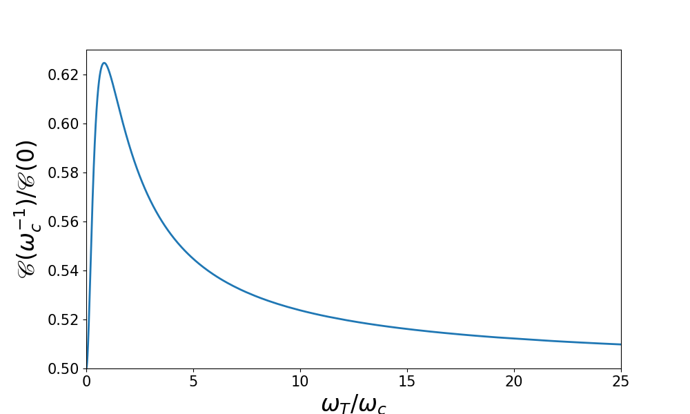
Figure 1: $\mathscr{C}\left(1/\omega_{c}\right)/\mathscr{C}\left(0\right)$ as a function of $\omega_{T}/\omega_{c}$, showing that we can use $t_{c}\propto 1/\omega_{c}$ as a guide to defining a legitimate boson bath correlation time since $\mathscr{C}\left(1/\omega_{c}\right)/\mathscr{C}\left(0\right)\rightarrow 1/2$ for $\omega_{T}\ll\omega_{c}$ and for $\omega_{T}\gg\omega_{c}$. We also see that even when $\omega_{T}\approx\omega_{c}$ we still can use $t_{c}\approx 1/\omega_{c}$ as a good estimate of the bath correlation time. To ensure a margin of safety to have the correlation low enough at $t_{c},$ here we define the boson field correlation time as $t_{c}=2\pi/\omega_{c}$.

II.2 Purification Process

As exposed, our main objective in this manuscript is to determine the optimal control Hamiltonian that, despite the environmental perturbations, evolves any initial qubit state $\rho_{IS}\left(0\right)$ to a target state $U_{\tau}\rho_{IS}\left(0\right)U_{\tau}^{\dagger},$ where $U_{\tau}$ is a target single-qubit operator, that is, $U_{\tau}\in\mathrm{SU}\left(2\right).$ By optimal we mean that we have a cost function associated with the way we choose the control Hamiltonian of Eq. (2) such as, for instance, when we want the least use of total energy during the quantum operation, from $t=0$ to $t=\tau,$ which is specified by the circuit requirements where the gate is to function and deliver the intended action on the qubit state. Ideally, the optimal control would evolve a pure state $\rho_{IS}\left(0\right)$ to the intended pure state $U_{\tau}\rho_{IS}\left(0\right)U_{\tau}^{\dagger},$ in which case, for perfect compensation against the noise, we would have a qubit state $\left|\psi\left(0\right)\right\rangle$ transformed to $U_{\tau}\left|\psi\left(0\right)\right\rangle,$ where $\rho_{IS}\left(0\right)=\left|\psi\left(0\right)\right\rangle\left\langle\psi\left(0\right)\right|.$

We notice that the perturbations mix the qubit state and we do not obtain the desired target evolution, admitting that the control protocol is not perfect. A possible function to consider is the usual Uhlmann-Jozsa fidelity measure defined by [37, 38]

$$\mathcal{F}_{UJ}\left(\rho,\sigma\right) = \left[\mathrm{Tr}\left(\sqrt{\sqrt{\rho}\sigma\sqrt{\rho}}\right)\right]^{2}.$$ (17)

Then the cost function can be taken to be the infidelity defined by $1-\mathcal{F}_{UJ}\left(\rho,\sigma\right)$, where we take $\sigma=U_{\tau}\rho_{IS}\left(0\right)U_{\tau}^{\dagger},$ the desired output, and $\rho=\rho_{IS}\left(\tau\right),$ obtained by solving Eq. (5).

The procedure to determine the optimal control is to minimize the infidelity for all possible input states $\rho_{IS}\left(0\right),$ given a target $U_{\tau}.$ Further constraints imposed on the optimization can be incorporated into the definition of the cost function using Lagrange multipliers. For instance, if we want to get the least infidelity using the least amount of energy for the control fields, we can minimize the infidelity summed to the total work done by the control fields to get the closest to the desired output.

Despite this robust theoretical approach, quantum optimal control in general is a time-consuming computational task [9]. One obvious reason why an open quantum system takes longer to optimize than a closed one is apparent by the fact that in the open system case, given a target $U_{\tau},$ we have to cover the whole set of possible initial states $\rho_{SI}\left(0\right).$ On the contrary, in the closed system case we can consider only the optimal control Hamiltonian to obtain the evolution of the identity operator to the target $U_{\tau},$ since in this case the dynamics are unitary. As we intend to minimize the control field frequencies to minimize control energy, we approximately substitute the dynamics described by the master equation of Eq. (5) for a unitary problem. To emulate the boson perturbations we introduce the interaction with a single auxiliary qubit instead, as suggested in Chapter 8 of Ref. [39]. Here, however, we take into account the specific time dependence presented in Eqs. (13) and (14). Using this device we have an effective purified problem of a finite dimension whose master equation, after tracing out the auxiliary qubit degrees of freedom, is given by

$$\frac{\mathrm{d}\rho_{IS}^{(e)}\left(t\right)}{dt} = -\frac{h\left(t\right)}{\hbar^{2}}\int_{0}^{t}\mathrm{d}t^{\prime}\,h\left(t^{\prime}\right)\left[S\left(t\right),\left[S\left(t^{\prime}\right),\rho_{IS}^{\left(e\right)}\left(t^{\prime}\right)\right]\right],$$ (18)

where $\rho_{IS}^{(e)}\left(t\right)$ is the effective reduced density matrix of the qubit and we define the function $h\left(t\right)$ as

$$h\left(t\right) = \frac{\hbar\dot{\mu}\left(t\right)}{2\sqrt{1-\mu^{2}\left(t\right)}}.$$ (19)

To derive Eq. (18) we use $S\left(t\right)$ as given by Eq. (7), $\mu\left(t\right)$ as defined in Eq. (14), and instead of the Hamiltonian of Eq. (3), we keep the same $H_{c}\left(t\right)$ and define an effective Hamiltonian as

$$H_{e}\left(t\right) = H\left(t\right)+H_{D}\left(t\right),$$ (20)

with

$$H\left(t\right) = H_{c}\left(t\right)\otimes I$$ (21)

and a drift Hamiltonian given by $H_{D}\left(t\right)=-h\left(t\right)\sigma_{z}\otimes\sigma_{z}$ or, using Eq. (19),

$$H_{D}\left(t\right) = -\frac{\hbar\dot{\mu}\left(t\right)}{2\sqrt{1-\mu^{2}\left(t\right)}}\sigma_{z}\otimes\sigma_{z}.$$ (22)

Here $I$ stands for the $2\times 2$ identity matrix. In the absence of control and if in this case $H_{c}\left(t\right)\propto\sigma_{z},$ both Eqs. (5) and (18) give the same final reduced density matrix for the same initial qubit state, with the proviso that we have to adopt $\left|\psi_{\text{aux}}\left(0\right)\right\rangle=\left(\left|0\right\rangle+\left|1\right\rangle\right)/\sqrt{2},$ where $\sigma_{z}\left|0\right\rangle=\left|0\right\rangle$ and $\sigma_{z}\left|1\right\rangle=-\left|1\right\rangle,$ as the initial state of the auxiliary qubit. The same statement is not true in general if we have a time dependent control present. There are two limiting situations in which both Eqs. (5) and (18) give the same answer: when the control Hamiltonian of Eq. (2) varies in a time scale long enough as compared to $t_{c}$ so that the approximation

$$S\left(t^{\prime}\right) \approx S\left(t\right)$$ (23)

is valid in Eqs. (5), (6), and (18), as we show in Appendix VI.1, and when the gate time $\tau$ is short enough with the correlation time $t_{c}$ long enough that the approximations $B\left(t^{\prime}\right)\approx B\left(t\right),$ $h\left(t^{\prime}\right)\approx h\left(t\right),$ and $\omega_{c}t\ll 1,$ are valid in Eqs. (5) and (18), as we show in Appendix VI.2. Thus, since we apply this solution in the context of CDD, i.e., within the long correlation time regime, the approximation holds true and Eqs. (5) and (18) are equivalent.

II.3 Formulation of the control theory

A time-dependent single-qubit gate can be seen as a quantum circuit of gradually-changing instantaneous (ideal) single-qubit gates, if we use a regular partition of the scheduled time interval [40]. Accordingly, let us use a simple cost function to minimize. We know that the integral of the square root of the control Hamiltonian bounds the circuit complexity [41, 42, 43]. We can, however, use the integral over the square of the control Hamiltonian as our cost function, for the sake of simplicity, since then minimizing such a cost function will also minimize the conventional one with the square root of the control Hamiltonian [44]. Our aim is then to minimize our cost function with the implicit assumption that the time evolution of the identity operator to the target unitary operator satisfies, at each instant, the Schrödinger equation with the effective total Hamiltonian given by Eq. (20). We can simplify the formulation of the control problem by using, at each instant, a Lagrange multiplier that constrains the instantaneous unitary operator to be given by the Schrödinger equation. In the functional to minimize, we then use an integral over the constraint equation summed to the integral of the square of the effective Hamiltonian:

$$J\left(H,U,\Lambda\right) = \int_{0}^{\tau}\mathrm{d}t\,\mathrm{Tr}\left[\frac{1}{2}H\left(t\right)H\left(t\right)+\Lambda\left(t\right)\left(i\hbar\frac{dU\left(t\right)}{dt}U^{\dagger}\left(t\right)-H_{e}\left(t\right)\right)\right],$$ (24)

where we adopt the convention of using the normalized trace, that is, $\mathrm{Tr}\left(I\right)=1$ for any square matrix dimension, $\tau$ is the time interval corresponding to the scheduled duration of the required gate operation, $\Lambda\left(t\right)$ is the co-state (the matrix containing the instantaneous Lagrange multipliers), and we now use $H\left(t\right),$ $U\left(t\right),$ and $\Lambda\left(t\right)$ as the functions to be varied independently to minimize the functional $J\left(H,U,\Lambda\right).$ According to Pontryagin’s Maximum Principle [45], the control Hamiltonian $H\left(t\right)$ that minimizes Eq. (24) is also the optimal Schrödinger equation solution that minimizes the total energy spent during the interval $\tau$ because it minimizes the integral of the square of $H\left(t\right).$

We write the factor multiplied by $\Lambda\left(t\right)$ with $\left[\mathrm{d}U\left(t\right)/\mathrm{d}t\right]U^{\dagger}\left(t\right)$ because this quantity is an anti-Hermitian traceless matrix and, therefore, belongs to the Lie algebra $\mathfrak{su}\left(2^{2}\right)$ and not to the Lie group $\mathrm{SU}\left(2^{2}\right)$ as does $U\left(t\right),$ so that Eq. (24) is mathematically consistent. Because the control is described by the Hamiltonian of Eq. (21), we have a sub-Riemannian geometry [44], since the control Hamiltonian does not operate in all the directions spanning the whole Lie algebra $\mathfrak{su}\left(2^{2}\right).$ Actually, in the absence of a control, the Schrödinger evolution is restricted to be generated by the drift Hamiltonian, Eq. (22), that does not drive the system out of the one-dimensional subspace of $\mathfrak{su}\left(2^{2}\right)$ generated by $\sigma_{z}\otimes\sigma_{z}.$ Moreover, because we are restricted to control only the physical qubit and not the auxiliary one, our control subspace is spanned by the three-dimensional distribution

$$\Delta = \left\{\sigma_{x}\otimes I,\sigma_{y}\otimes I,\sigma_{z}\otimes I\right\}.$$ (25)

The effective total Hamiltonian, Eq. (20), can only drive the system into the sub-algebra of $\mathfrak{su}\left(2^{2}\right)$ generated by the six-dimensional subspace

$$\Gamma = \Delta\cup\left\{\sigma_{x}\otimes\sigma_{z},\sigma_{y}\otimes\sigma_{z},\sigma_{z}\otimes\sigma_{z}\right\}.$$ (26)

The reachable sub-group is then obtained through the exponentiation of the sub-algebra elements multiplied by a real number. The subset $\Gamma$ generates a sub-algebra because this generated subspace contained in $\mathfrak{su}\left(2^{2}\right)$ is closed under the commutator operation between its elements. In other words, the control Hamiltonian does not belong to the same subspace as the drift Hamiltonian, Eq. (22), and this fact complicates our control problem [9].

The geodesic equations we obtain by functional minimization of Eq. (24) are given by [46, 47, 48]

$$i\hbar\frac{\mathrm{d}U\left(t\right)}{\mathrm{d}t} = H_{e}\left(t\right)U\left(t\right),$$ (27)

$$i\hbar\frac{\mathrm{d}\Lambda\left(t\right)}{\mathrm{d}t} = \left[H\left(t\right),\Lambda\left(t\right)\right],$$ (28)

and

$$\mathcal{P}\left[\Lambda\left(t\right)\right] = H\left(t\right),$$ (29)

where $\mathcal{P}$ is the projector onto the sub-Riemannian subspace spanned by the distribution $\Delta,$ Eq. (25). We notice that the co-state belongs to the sub-algebra spanned by $\Gamma,$ Eq. (26). We can join Eqs. (27), (28), and (29) into a single equation:

$$i\hbar\frac{\mathrm{d}U\left(t\right)}{\mathrm{d}t} = \left\{H_{D}\left(t\right)\right.$$ (30)

$$\left.+\mathcal{P}\left[U\left(t\right)\Lambda\left(0\right)U^{\dagger}\left(t\right)\right]\right\}U\left(t\right).$$

The algorithm we must follow is to try and find $\Lambda\left(0\right)$ that, at $t=\tau,$ gives the desired target unitary operator $U_{\tau}\otimes I$ as the solution $U\left(\tau\right)$ obtained by solving Eq. (30). The essential difficulty with finding $\Lambda\left(0\right)$ from Eq. (30) is that we would have to invert the projector $\mathcal{P},$ which is not uniquely determined: there are infinitely many possible solutions for $\Lambda\left(0\right)$ giving the same projection of $U\left(t\right)\Lambda\left(0\right)U^{\dagger}\left(t\right)$ for any given $U\left(t\right).$ Even if we use a Riemannian geometry with a metric that penalizes the directions orthogonal to the ones in the distribution $\Delta,$ thus avoiding the projector inversion problem, we still would not have $\mathrm{d}U\left(t\right)/\mathrm{d}t$ at $\tau,$ being now obliged to face this other indeterminacy. Hence, we choose to try many initial co-states $\Lambda\left(0\right)$ and locate the one that renders the solution of Eq. (30), $U\left(\tau\right),$ that is closest to the required target $U_{\tau}\otimes I.$ As a distance between two unitary operators here we adopt the infidelity measure, given by the fidelity, as defined in Ref. [49], subtracted from the real unit:

$$\mathcal{I}\left(U_{1},U_{2}\right) = 1-\left|\mathrm{Tr}\left(U_{1}^{\dagger}U_{2}\right)\right|,$$ (31)

where we use the normalized trace.

II.4 Optimal Hamiltonian

Our aim is to be able to efficiently obtain the co-state $\Lambda\left(0\right)$ once we are given a target $U_{\tau}\otimes I.$ However, the algorithm we described is based on searching for the minimum of $\mathcal{I}\left(U_{\tau}\otimes I,U\left(\tau\right)\right),$ Eq. (31), viewed as a noninvertible map that takes $\Lambda\left(0\right)$ to $U\left(\tau\right)$ through Eq. (30). For a given target this search can take a relatively long time, depending on the required level of accuracy required. Here, we show how to compute $\Lambda\left(0\right)$ using a brute-force approach, employing a computationally demanding process named $q\text{-jumping}$ [9]. In Sec. III, after calculating a sufficient number of cases by means of the $q\text{-jumping}$ strategy, we then train a neural network to predict $\Lambda\left(0\right)$ for each given target $U_{\tau}\otimes I$. As we will show, these predictions can give estimates that are not only quickly calculated, but also much closer to the desired answer.

The initial guess for $\Lambda\left(0\right)$ is important since it helps to find one that is the closest to the one that minimizes the infidelity, Eq. (31). If we could invert the projector operator in $\mathcal{P}\left[U\left(t\right)\Lambda\left(0\right)U^{\dagger}\left(t\right)\right]$ in Eq. (30), then we could easily find an initial guess for the searching algorithm. The idea would be to initially write $U_{\tau}=\exp\left(-iH_{\text{guess}}\tau/\hbar\right),$ then we would calculate $H_{\text{guess}}$ and use $H_{\text{guess}}=H_{D}\left(0\right)+\mathcal{P}\left[\Lambda\left(0\right)\right]$ to find an initial guess for $\Lambda\left(0\right),$ but we can not invert $\mathcal{P}.$ To avoid this problem we proceed in an alternative way. We use a Riemannian geometry with penalty factors along the directions in $\Gamma,$ Eq. (26), that do not belong to the distribution $\Delta,$ Eq. (25). Inspired by the methodology of Ref. [9], our formulation is as follows.

For our purposes we use a single penalty factor, $q,$ along the directions in the difference set:

$$\Gamma\backslash\Delta = \left\{\sigma_{x}\otimes\sigma_{z},\sigma_{y}\otimes\sigma_{z},\sigma_{z}\otimes\sigma_{z}\right\}.$$ (32)

We now define a control Hamiltonian that includes all six directions of $\Gamma:$

$$H_{q}\left(t\right) = \sum_{k=1}^{3}\alpha_{k}\left(t\right)\sigma_{k}\otimes I+\sum_{k=1}^{3}\beta_{k}\left(t\right)\sigma_{k}\otimes\sigma_{z},$$ (33)

where $\left(\sigma_{1},\sigma_{2},\sigma_{3}\right)=\left(\sigma_{x},\sigma_{y},\sigma_{z}\right)$ and $\alpha_{k}\left(t\right),\beta_{k}\left(t\right)$ for $k=1,2,3,$ are real functions of time. Now we proceed analogously as when we minimized Eq. (24), except that now, instead of the square of the control Hamiltonian in the integrand, we use $G_{q}\left(H_{q}\left(t\right),H_{q}\left(t\right)\right),$ where, given two Hamiltonians, $H_{A}$ and $H_{B},$ we define the Riemannian metric

$$G_{q}\left(H_{A},H_{B}\right) = \frac{1}{2}\sum_{k=1}^{3}\mathrm{Tr}\left[H_{B}\left(\sigma_{k}\otimes I\right)H_{A}\right]$$ (34)

$$+\frac{q}{2}\sum_{k=1}^{3}\mathrm{Tr}\left[H_{B}\left(\sigma_{k}\otimes\sigma_{z}\right)H_{A}\right],$$

where $q$ is a finite positive real number. By increasing $q,$ the equations that give the geodesic must converge to the desired case of our sub-Riemannian metric where the control is in the form of Eq. (2), since the solution to the minimization problem gives $\beta_{k}\left(t\right)\rightarrow 0,$ for $k=1,2,3,$ as $q\rightarrow\infty.$

The new geodesic equation obtained for a finite $q$ is given by

$$i\hbar\frac{\mathrm{d}U_{q}\left(t\right)}{\mathrm{d}t} = \left\{H_{D}\left(t\right)\right.$$ (35)

$$\left.+\mathcal{F}_{q}\left[U_{q}\left(t\right)\Lambda_{q}\left(0\right)U_{q}^{\dagger}\left(t\right)\right]\right\}U_{q}\left(t\right),$$

with a new invertible operator, for finite $q,$ defined by

$$\mathcal{F}_{q} = \mathcal{P}+\frac{1}{q}\mathcal{Q},$$ (36)

where $\mathcal{P}$ is the same projector of Eq. (29), that projects onto the subspace spanned by the distribution $\Delta,$ while $\mathcal{Q}$ is the projector onto the subspace spanned by $\Gamma\backslash\Delta,$ Eq. (32). The operator $\mathcal{F}_{q}$ is not a projector for finite $q,$ but $\mathcal{F}_{q}\rightarrow\mathcal{P}$ as $q\rightarrow\infty.$

We start with $q=10$ and, for each target $U_{\tau}$ generated according to Eq. (37), we write $U_{\tau}=\exp\left(-iH_{\text{guess}}\tau/\hbar\right)$ and calculate $H_{\text{guess}}.$ Then we impose $H_{\text{guess}}=H_{D}\left(0\right)+\mathcal{F}_{q=10}\left[\Lambda_{q=10}\left(0\right)\right]$ to find an initial guess for $\Lambda_{q=10}\left(0\right),$ since we can invert $\mathcal{F}_{q=10}.$ Numerically, we can use, for instance, FindMinimum in Wolfram Language or scipy.optimize.minimize in Python to discover, from our initial guess, a better $\Lambda_{q=10}\left(0\right)$ that minimizes the infidelity, Eq. (31). The first trial sometimes takes a relatively long time, depending on the target $U_{\tau},$ and in some cases the infidelity is hardly as low as we require. We then refine the result by using a shooting algorithm based on the Newton method to find the value of $\Lambda_{q=10}\left(0\right),$ starting from the output of FindMinimum or scipy.optimize.minimize, that is a zero of the infidelity.

We then iterate the process named $q\text{-jumping}$ in Ref. [9] by using the refined $\Lambda_{q=10}\left(0\right)$ as an initial guess for the evolution for the case with $q>10.$ The iteration process proceeds by increasing $q$ by an increment $\Delta q$ and using $\Lambda_{q}\left(0\right)$ obtained from the previous iteration as a first guess for the evolution with a new penalty factor of $q+\Delta q.$ After numerically minimizing, if the infidelity is not low enough (we could pick a tolerance on the order of $10^{-5},$ for instance), we use the shooting algorithm to improve the result for $\Lambda_{q+\Delta q}\left(0\right).$ Sometimes, however, depending on the target $U_{\tau},$ the minimization is not near enough to the minimum of the infidelity that the shooting method diverges even further from the minimum of Eq. (31). In such cases we keep the $\Lambda_{q+\Delta q}\left(0\right)$ that we had as output of the numerical minimization.

The choice of $\Delta q$ for each iteration is multiplicative and it is not fixed. Because after a gradual increase to a certain value of $q$ the difference between $\mathcal{F}_{q}$ and $\mathcal{P}$ becomes small enough, the jump from a large enough $q$ to $q\rightarrow\infty$ becomes easily implemented. However, for intermediary values of $q,$ typically lower than $100,$ the jumps have to be smaller than for $q>100$ between one iteration and the next. We, therefore, by trial and error, define a way to increase $q$ in a multiplicative way so that after a chosen number of iterations, $N_{\text{it}},$ we reach a maximum $q=q_{\text{max}}$ value of at least $2000$ or more (up to $10000$ in some easier cases), using a multiplicative factor $10^{\chi}$ with $\chi=\log_{10}\left(q_{\text{max}}/q_{\text{in}}\right)/N_{\text{it}},$ where $q_{\text{in}}$ is the initial $q$, which in the present description we picked as $q_{\text{in}}=10.$ If, depending on the target $U_{\tau}$, the required tolerance is not reached, we use a decreasing multiplicative factor and retake the iteration step so that we try and see if with a lower increase of $q$ the guess is good enough to converge to a lower infidelity than with the previous intended $q$ increment. Because of this some easier cases reach up to, say, $q=10000$ with good fidelity after $N_{\text{it}},$ while other, more difficult cases, do not even reach, with low enough infidelity, the minimum desired $q=2000.$ For difficult cases, we then run another pass starting over from the beginning, with $q=10,$ with even lower increments of $q$ between iterations. After painstakingly determining $\Lambda_{q_{\text{max}}}\left(0\right)$ with high enough fidelity, we run the sub-Riemannian dynamics to take the $q\text{-jump}$ to infinity using the evolution given by Eq. (30) with $\Lambda_{q_{\text{max}}}\left(0\right)$ as initial guess. Thus, after this quite demanding computational effort, we determine $\Lambda\left(0\right)$, which provides the optimal field control for any quantum gate. This result marks an advancement in the CDD strategy, since once the environment is well characterized, an optimal control field can be determined with high precision.

III Neural Network

As we mentioned above, the computational effort needed to compute a single gate is considerable. This becomes particularly problematic in the context of circuit optimization, where on-demand logical gates are essential. To treat this problem, we develop a neural network that can learn from previous results.

We begin generating an initial population of $2000$ quantum gates using

$$U_{\tau} = I\cos{\theta}-i\mathbf{\hat{u}}\boldsymbol{\cdot}\boldsymbol{\sigma}\sin{\theta},$$ (37)

where the values of the versor $\mathbf{\hat{u}}$ are randomly chosen to basically cover the whole unit sphere and the values of $\theta$, also randomly picked, cover the upper half of the unit circumference. Then, instead of using $U_{\tau}$, we store only the values of $\theta\mathbf{\hat{u}}$, since we can easily recover the target unitary operator by using $U_{\tau}=\exp\left(-i\theta\mathbf{\hat{u}}\boldsymbol{\cdot}\boldsymbol{\sigma}\right).$

Because $\Lambda\left(0\right)$ is a Hermitian matrix given as a linear combination of the elements in $\Gamma,$ Eq. (26), we only store the six corresponding real coefficients. Our aim is then to find these six real quantities once we are given the three real values $\theta\mathbf{\hat{u}}$ defining the target $U_{\tau}.$ Naturally, we train and test this neural network to, afterward, guess target cases not in the initial training set of nearly $2000$ cases (some cases could not reach high enough fidelity). We then check the infidelity of the guessed $\Lambda\left(0\right)$ using it as an initial value in Eq. (30) and, when necessary, we use numerical minimization as before to refine the result to a tolerable infidelity. Now, however, it turns out that the process of guessing, deciding if refinement is necessary, and eventual refinement is much faster than the cumbersome $q\text{-jumping}$ algorithm we described. In the next subsections, we present the results of our investigations.

III.1 Simple Example

To illustrate all the steps of the procedure we described in the previous section, let us consider a single case. In the following, we use the target unitary operator given by Eq. (37), namely,

$$U_{\tau} = \exp\left(-i\theta\mathbf{\hat{u}}\boldsymbol{\cdot}\boldsymbol{\sigma}\right),$$

with

$$\theta\mathbf{\hat{u}} = 0.307485\mathbf{\hat{x}}+0.346931\mathbf{\hat{y}}-2.78627\mathbf{\hat{z}}.$$ (38)

In the code, the complete $U_{\tau}\otimes I$ unitary operator is represented only by the coefficients $u_{k}$ in $(0.307485,0.346931,-2.78627,0,0,0),$ since using the elements $\gamma_{k}$ of $\Gamma,$ Eq. (26), namely, $\sigma_{k}\otimes I,$ for $k=1,2,3,$ and $\sigma_{k-3}\otimes\sigma_{z},$ for $k=4,5,6,$ we have

$$U_{\tau}\otimes I = \exp\left(-i\sum_{k=1}^{6}u_{k}\gamma_{k}\right).$$

According to Sec. II.4, we next change the previous code vector to $(0.307485,0.346931,-2.78627,0,0,qh\left(0\right)),$ now storing the coefficients for $\left[H_{\text{guess}}-qH_{D}\left(0\right)\right],$ and we use these components as coefficients of the $\Gamma$ basis matrices to define our initial guess for $\Lambda_{q=10}\left(0\right).$

Our code took about forty minutes to run $100$ jumps, on one of our desktop computers, and we ended up propagating $q$ up to the value $q=41.9348,$ reaching infidelity of $0.0000999889,$ and giving a $\Lambda_{q}\left(0\right)$ stored in code with coefficients $(1.11881,0.891343,0.277546,-1.84379,1.09701,-19.2034).$ For this calculation, we used a maximum infidelity tolerance of $10^{-4}.$

We then can take the result of the previous calculation and restart the $q\text{-jumping,}$ now relaxing the tolerance to, say, $5\times 10^{-3}.$ After other $100$ jumps we ended up with $q=2000,$ reaching an infidelity of $0.000728164,$ and obtaining a $\Lambda_{q}\left(0\right)$ stored in code as $(9.74364,0.542157,0.57394,5.52942,-22.2162,-39.9236).$ This calculation took about $57$ minutes on the same desktop computer.

We can now continue the $q\text{-jumping}$ process using the same tolerance of infidelity, up to $5\times 10^{-3},$ taking now $200$ jumps from $q=2000$ to $q=10000.$ This run took about $76$ minutes, reaching an infidelity of $0.000661113,$ and resulting in a $\Lambda_{q}\left(0\right)$ stored as $(10.5295,0.382698,0.557801,5.30813,-24.297,-44.0305).$ From this result now we run the jump for the limit in which $q$ tends to an infinite value, obtaining $\left(10.5288,0.38277,0.557781,5.30812,-24.297,-44.0307\right),$ with an infidelity of $0.000674937.$ The jump to $q\rightarrow\infty$ is much faster: this one took only $22$ seconds.

III.2 Neural network predictions

To make use of neural networks, as inspired by Refs. [46, 48], we built many models searching for a good architecture. In contrast to both authors, we did not make use of recurrent neural networks. Instead, we built a simple fully connected perceptron [50, 51] and changed its hyperparameters in order to find good predictors, making use of both dropout techniques as well as l2 regularization methods to avoid overfitting.

We want to predict the relationship between $\lambda_{k}$, such that $\Lambda(0)=\sum_{k=1}^{6}\lambda_{k}\gamma_{k}$, and each of the desired $u_{k}$. Therefore, we designed the network to use $u_{k}$ as its input, and predict the components $\lambda_{k}$. The loss used in training is the usual MSE.

We trained a neural network model using the population of $2000$ targets, using it to predict the costate $\Lambda(0)$ that generates the vector shown in Eq. (38). The model itself took around $0.1$ second to obtain a prediction for the costate, and the infidelity of said prediction is around $0.33$. However, with this prediction we can use scipy.optimize.minimize in order to refine $\Lambda(0)$, taking about $90$ seconds to obtain an infidelity of $\approx 9.2\times 10^{-11}$. Notice that we can use the model to predict in seconds new unitaries that would take hours by using the $q$-jumping method.

With the $2000$ targets, we can start a process of data augmentation by using the said network itself. To do so, we generate $100$ new unitary targets, find initial guesses with the network, process them through the minimization algorithm, and add them to the dataset. This dataset is used to train the network once again, using only the data that obtained infidelity smaller than the chosen threshold. This process was repeated until our model had around $6000$ data points available for training. With the new data, we trained yet another model, separating around a third of the data as test-only.

With all the new data, we looked for a new model that fits nicely to our data, predicting small infidelities for the desired unitaries. In particular, the specific model has $5$ hidden layers, all using a rectified linear function as their activation function, as well as a dropout rate of $30\%$ and an l2 parameter of $0.002$.

Afraid of obtaining biased results due to few data - even with the augmentation -, we trained the network by applying a k-fold cross-validation test. [50, 51] The loss result is shown in Fig. 2. We notice a plateau in the validation loss around $200$ epochs. The chosen loss is the usual MSE.

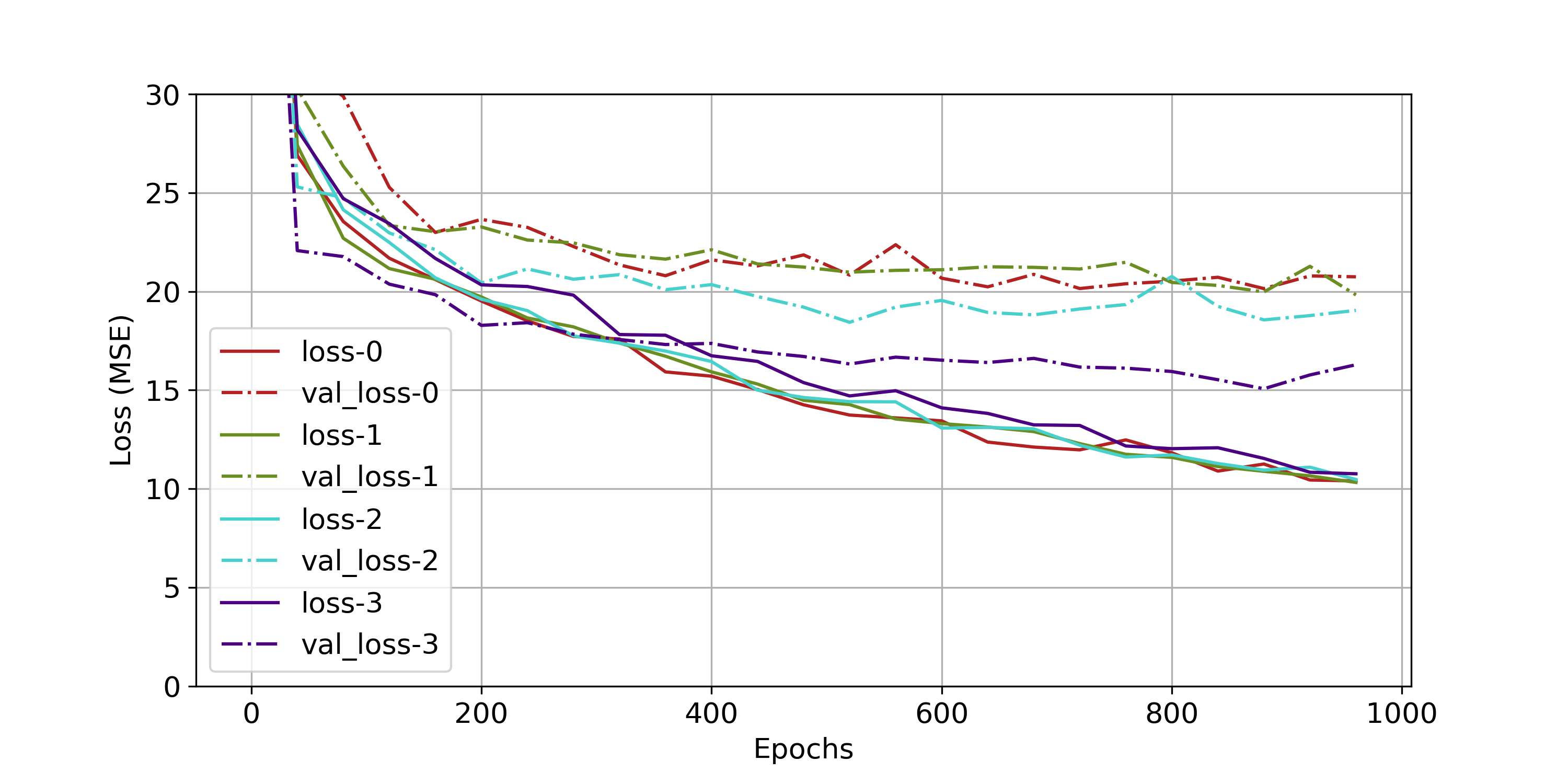
Figure 2: Training (continuous line) and validation (dashed line) losses for the neural network training process. With a small dataset, we decided to make use of the $k$-fold cross-validation technique for $k=4$. We notice that the validation loss does not decrease after $200$ epochs.

Then, we trained the same model on all available data, with the loss presented in Fig. 3. This plot shows the training loss continuously decreasing in all training, while the validation loss gets stagnant around $200$ epochs as said previously.

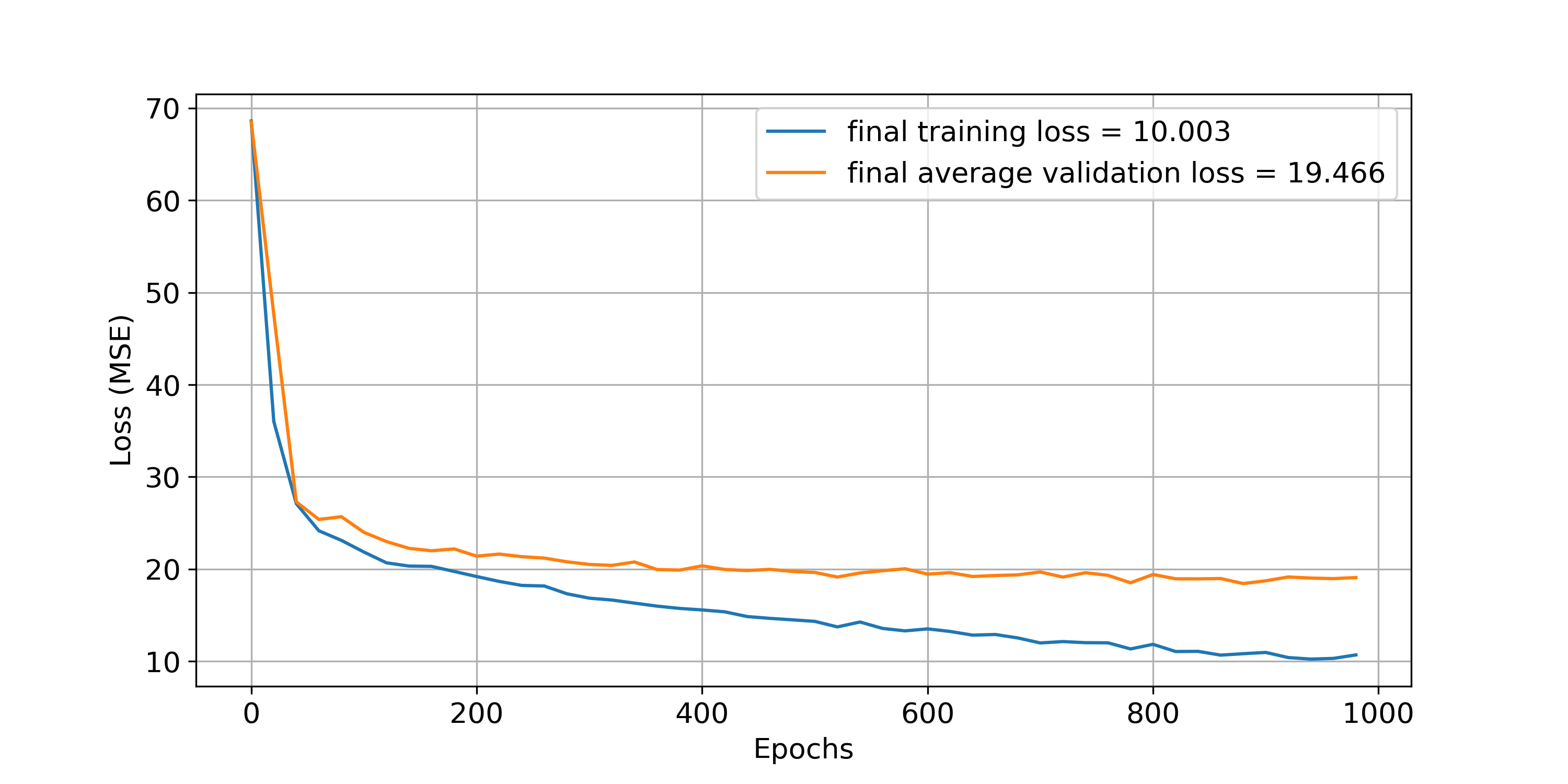
Figure 3: Training loss (blue) using all available data on training, compared to the average validation loss (orange) obtained in the $k$-cross validation shown previously.

With this neural network model, we compute the infidelities the unitaries predicted both using the training dataset, as well as the test dataset - data that the network has never seen before, not even in validation steps. Such infidelities are presented in Fig. 4, reaching as low as $10^{-4}$. About 63% of the data is present on the smallest infidelity bin for the training dataset and 59% for the test dataset. This means that the output from the network, in many cases, does not need to be significantly improved, although the optimization of such a guess is fast.

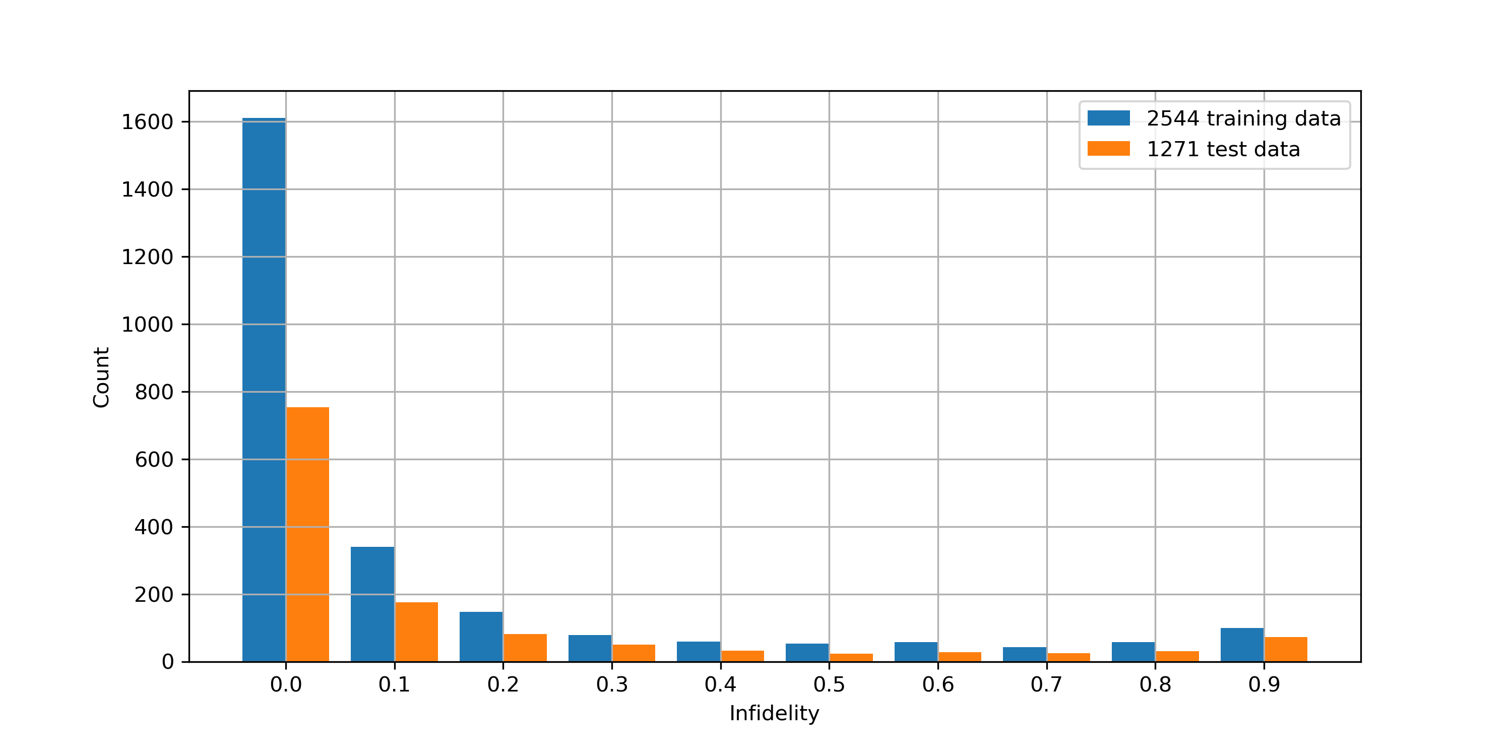
Figure 4: Histogram of infidelities in logarithmic scale. The first bin - which amounts to around 63%/59% of the training/test data - comprehends infidelities from $10^{-4}$ up to $10^{-1}$. This indicates the neural network predictions are, in general, great guesses in order to use other numerical minimization tools.

In Fig. 5, we show the relation True vs. True for $\lambda_{\text{target}}$ and $\lambda_{\text{pred}}$ for the test dataset. In this plot, the closer the data is to the identity curve, the better the overall prediction of the network. Notice that the prediction is accurate to the target values as most of the points are close to the identity curve. In particular, we notice that the $\lambda_{6}$ components are skewed. This happens because of the existence of the external Hamiltonian, which drifts the system towards negative values of $\sigma_{z}\otimes\sigma_{z}$.

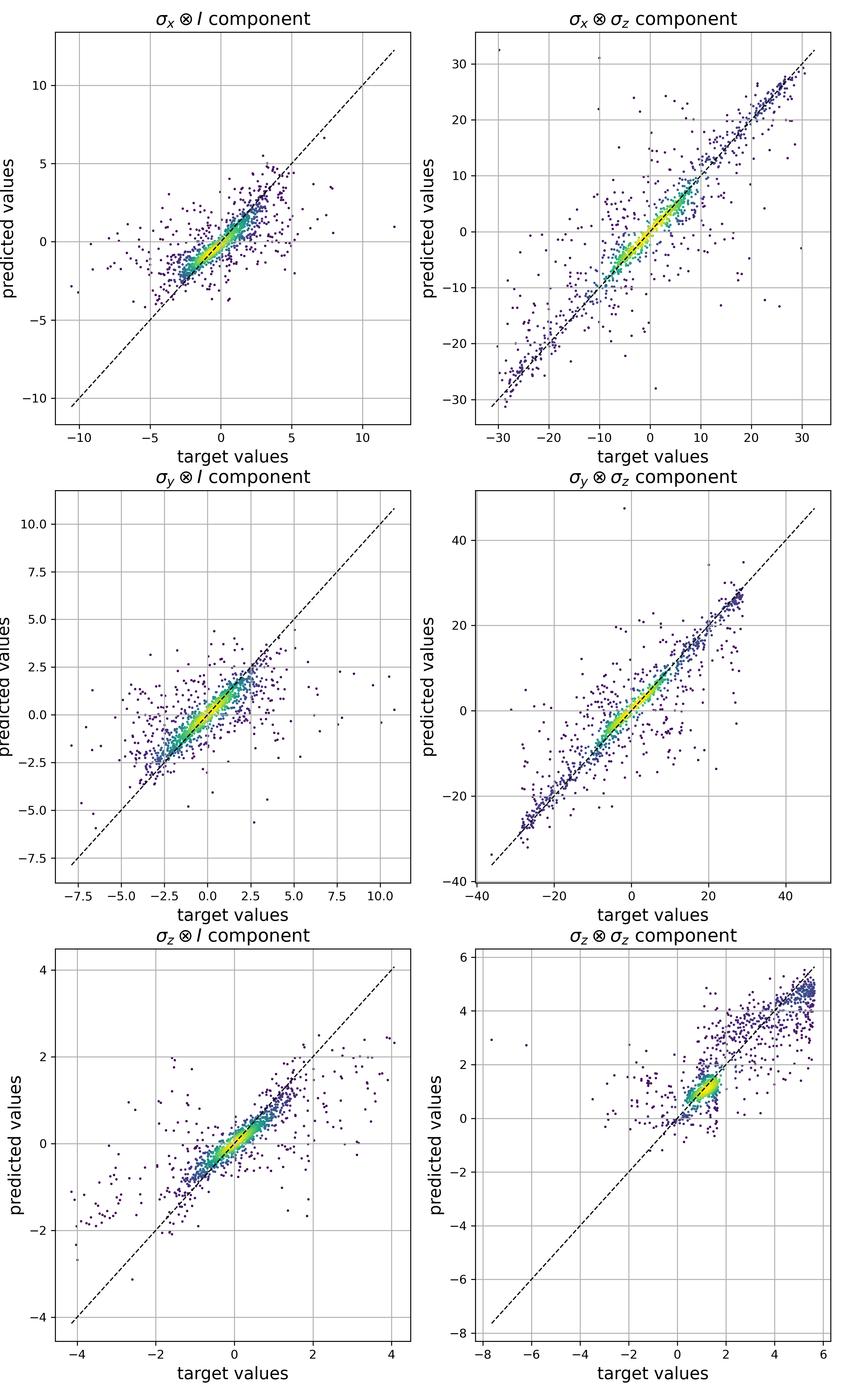
Figure 5: Scatter plot in which we compare the predicted values with the true values for each component $\lambda_{k}$, using the test dataset. We notice that most components follow the identity curve with little variance. Notice that the off-control components reach higher values than the control ones, taking into account the existence of the drift Hamiltonian. The $\lambda_{6}$ components are skewed, probably due to the drift Hamiltonian having the form $H_{D}(t)=-h(t)\sigma_{z}\otimes\sigma_{z}$. The color indicates density.

With the model doing a good prediction of a few thousand random unitaries, we now take a look at real gates used in usual quantum computing.

IV Results

With the neural network trained with around 6000 points, we tried reproducing four one-qubit gates. We choose the known Hadamard, $X$, and $T$ gates (the latter is given by $Z^{1/4}$), as well as the target unitary operator described by the vector in Eq. (38), which we will call $U_{G}$. The steps are as follows: we get the predicted costate for the four gates from the neural network, then use scipy.optimize.minimize to get an ideal costate $\Lambda(0)$ for each gate. We then calculate the time evolution operator with Eq. (30) and obtain the effective time-dependent Hamiltonian through

$$H\left(t\right) = \mathcal{P}\left[U(t)\Lambda\left(0\right)U^{\dagger}\left(t\right)\right].$$ (39)

Next, we use each resulting time-dependent Hamiltonian to solve the master equation, given by Eq. (5). For all the gates we choose $\left(\ket{0}+\ket{1}\right)/\sqrt{2}$ as the initial state. The reason is that a state of maximum superposition is the most affected by dephasing noise. So in the interaction picture, if the density operator keeps all of its coherence terms intact by the end of the evolution, this means the method of protection is working.

Besides the evolution with the time-dependent Hamiltonian, we also solve the master equation with two other Hamiltonians in order to make comparisons. The first is with what we here call “trivial Hamiltonian”. This Hamiltonian is defined as the constant Hamiltonian which would generate the target unitary should noise not be present. In practical terms, it is directly obtained through

$$H_{\text{triv}} = i\hbar\log{U\left(\tau\right)}.$$ (40)

The second is the null Hamiltonian, that is, we solve the master equation with only noise acting on the system.

Since now we are analyzing the evolution of a density operator in the interaction picture, we quantify the fidelity, as a function of time, in terms of the initial density operator, that is,

$$F\left(t\right) = \mathrm{Tr}\left[\rho\left(0\right)\rho\left(t\right)\right].$$ (41)

This result follows immediately from the Uhlmann-Jozsa fidelity defined in Eq. (17) when at least one of the density operators is pure, and in this case $\rho\left(0\right)$ is always pure. Besides, since the analysis is made in the interaction picture, an ideally protected operation is identified as a density operator such that $\rho\left(0\right)=\rho\left(\tau\right)$, meaning $F\left(\tau\right)=1$, while the noisy operation is identified with $\rho\left(\tau\right)$ as a mixed state, meaning $F\left(\tau\right)<1$.

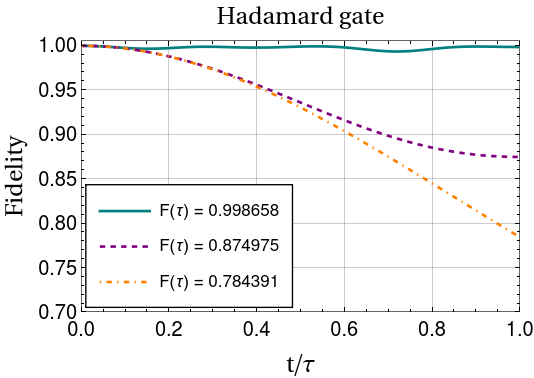
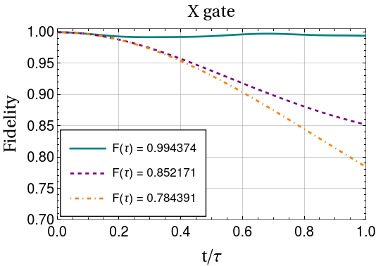
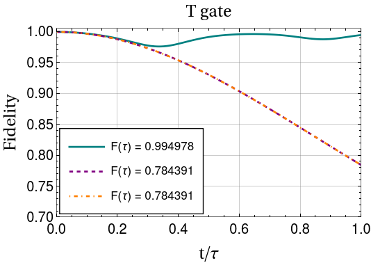
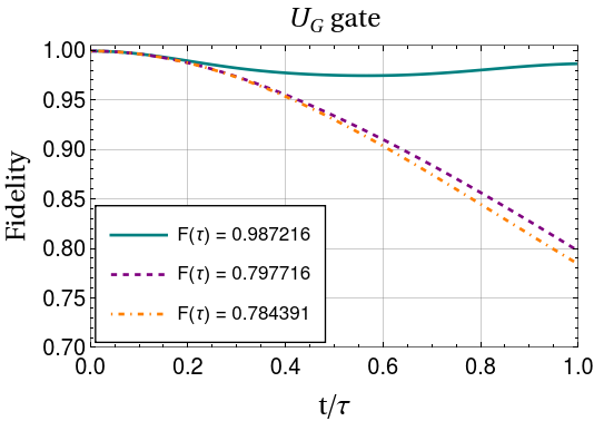
Figure 6: Fidelity as a function of time throughout the application of the quantum gates. The parameters chosen were $\eta=0.34$ and $\omega_{c}=\pi/(5\tau)$. The solid line is for the master equation solved with the optimal Hamiltonian, the dashed is for the trivial Hamiltonian and the dot-dashed is for the evolution due to noise exclusively. In the legends we show the fidelity at time $t=\tau$, that is, the gate fidelity.

To attest the validity of our strategy, we suppose the dephasing environment with $\eta=0.34$ and $\omega_{c}=\pi/\left(5\tau\right)$. As it was already mentioned, a longer correlation time, or equivalently, a lower $\omega_{c}$, places us in the CDD time regime, the ideal setting to test our optimal protective approach. The results for the fidelities of the four one-qubit gates are shown in Fig. 6. Notice that the evolution due to noise exclusively, represented by the dot-dashed lines, is the same for all gates since the acting noise is identical in all cases.

As observed, the lowest gate fidelity obtained via optimal control was $0.987216$ for the $U_{G}$ gate and the highest was $0.998658$, for the Hadamard gate. In comparison with the trivial Hamiltonian and the noise-free evolution, the fidelity by $t=\tau$ was bellow $0.8$ for the $U_{G}$ gate and around $0.87$ for the Hadamard gate. This represents a significant improvement. For the $T$ gate, the evolution due only to noise coincides with the one using the trivial Hamiltonian. The reason is that since it is just a phase gate, the trivial Hamiltonian is a constant proportional to $\sigma_{z}\otimes I$, and this commutes with the noise operator, proportional to $\sigma_{z}\otimes\sigma_{z}$. Therefore, when treated in the perspective of the interaction picture, the two-time evolutions are identical. In other words, the noise is indifferent when applying only $\sigma_{z}\otimes I$ on the qubit.

We can check, for the gates present in Fig. 6, the evolution of the density matrix plotted on the Bloch sphere. As shown in Fig. 7, starting at a pure state, the qubit travels inside the Bloch sphere due to the noisy gates, and emerges at its surface when the computation is complete. Thus, it mimics a unitary transformation within a noise environment. We also compare it with the ideal evolution, plotted in a dashed line.

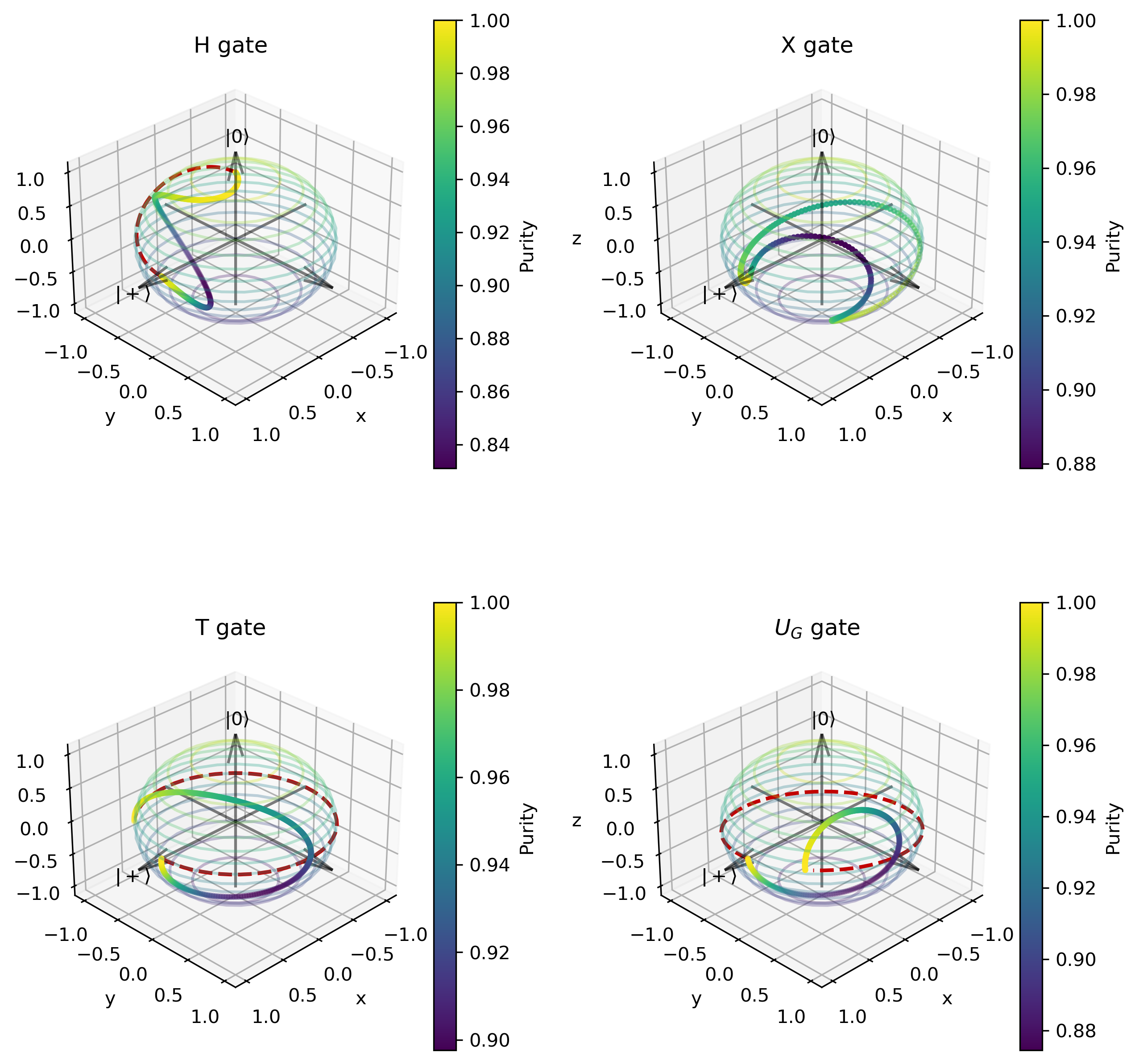
Figure 7: Evolution of the density matrix $\rho(0)=\op{+}{+}$ with the application of four gates. Color represents purity. The evolution begins with a pure state, traverses inside the Bloch sphere, in which the purity is less than one, and emerges at its surface at $t=\tau$, making sure that the gate mimics a unitary evolution. The dashed curves represent the ideal gate.

Now, it remains to verify how these obtained control fields compare, in energetic cost, with the fast-oscillating fields usually involved in the context of CDD, such as the methods described in [14, 17].

According to Eq. 24, we are calculating the energy cost for the implementation of a control Hamiltonian as

$$\mathcal{E}(H,U) = \frac{1}{2}\int_{0}^{\tau}\mathrm{d}t\,\mathrm{Tr}\left\{H(t)H(t)\right\}.$$ (42)

So after obtaining the optimal control (OC) fields for the four chosen quantum gates, we calculated the required control fields for them in the context of general continuous dynamical decoupling (GCDD) [14, 17], in order to compare the energetic cost between the two methods.

The motivation for this comparison is that, differently from the OC scheme, the Hamiltonian for the GCDD has the form $H(t)=H_{\text{gate}}+H_{c}(t)$, where the control $H_{c}(t)$ is a periodic operator whose period must be an integer multiple of the gate time and less than the noise correlation time, and $H_{c}(\tau)=I$. Therefore, since it is a method that involves rapidly oscillating fields, it is expected to be more costly, energetically speaking, than the optimal control scheme, and this is confirmed by the results shown in Table 1.

	$H$	$X$	$T$	$U_{G}$
OC	16.8959	13.5178	13.6184	4.76457
GCDD	396.018	396.018	384.992	468.800

Table 1: Energetic cost for executing the four gates: Hadamard ($H$), $X$, $T$ and $U_{G}$, using both methods: optimal control (OC) and general continuous dynamical decoupling (GCDD). All numeric values are in units of $\hbar$, meaning the actual energy is obtained by multiplying these values by $\hbar$.

As can be seen, the energies differ in magnitude between $10$ and $100$ times for the chosen gates. This is numerical evidence that the optimal control for dynamical decoupling presented here is indeed more efficient than usual methods involving fast-oscillating fields.

In order to compare the typical time profile dependence of the Hamiltonians we show, in Fig. 8, the three components of the control for the Hadamard gate in both methods: OC and GCDD. We also show the comparison in energy cost between the two methods in Fig 9, by plotting the energy function $\mathrm{Tr}\left\{H(t)H(t)\right\}/2=\left[H_{x}(t)^{2}+H_{y}(t)^{2}+H_{z}(t)^{2}\right]/2$. Besides confirming an improvement with respect to energy consumption, this figure, along with Fig. 8, shows that the derivatives of the control fields of OC are considerably smaller than the ones in GCDD. This suggests a more efficient regime for field variations, that is, less imprecision when turning the field on/off, as well as when changing the field to the configuration of another quantum gate, when applying several in sequence.

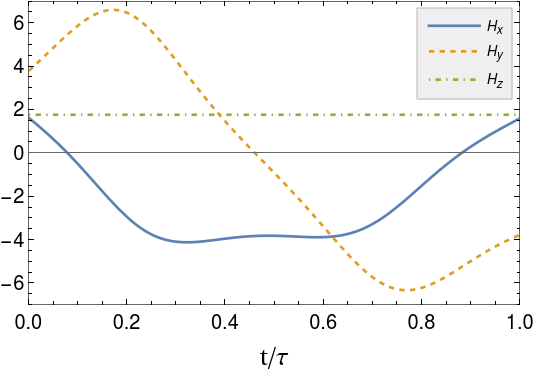
(a) OC

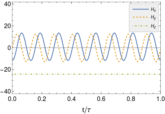
(b) GCDD

Figure 8: Components $\sigma_{x}$, $\sigma_{y}$ and $\sigma_{z}$ of the control Hamiltonian for both, optimal control and general continuous dynamical decoupling, for the Hadamard gate. The energy values in the y-axis are given in units of $\hbar$, meaning the actual energy is obtained by multiplying these numerical results by $\hbar$.

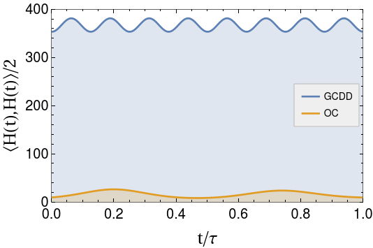
Figure 9: Time-dependent energy function $\mathrm{Tr}\left\{H(t)H(t)\right\}/2$ for both, optimal control and general continuous dynamical decoupling. The total energy cost in units of $\hbar$, according to Eq. 42, is given by the areas under the curves.

V Conclusion

We present an optimal control strategy designed for the CDD regime where the noise correlation time is long compared to the time scale in which the control fields can vary [4, 52, 49, 53, 54, 55]. In such situation, we use the time-dependent purification scheme we envisaged to emulate the noise through a unitary evolution, by introducing an auxiliary qubit to be traced over after the optimization is completed. We use a sub-Riemannian geometry framework for the two-qubit unitary group, to show that we can, in principle, implement any single-qubit gates in an efficient way despite the presence of dephasing noise. Our control fields, represented by continuous functions of time, can be used at the pulse level in the coding structure of current available quantum computers. Naturally, as exposed above, our optimal control requires previous spectroscopy of the environmental noise, which is obtainable by means of different techniques, including Ramsey spectroscopy and pulsed dynamical decoupling [19, 20, 21, 22, 23, 24, 25, 26].

Also, we train a neural network to efficiently estimate control Hamiltonians for any on-demand target unitaries covering the $\mathrm{SU}\left(2\right)$ unitary group. We show that, after having trained the neural network to guess the optimal control for a set of parameters, it can be used to guess the results for a new set of parameters, albeit sufficiently close to the previous ones, so that ulterior refinement produces corresponding high-fidelity optimal gates for the new parameters. Previous works using machine learning to enhance the efficiency of the production of on-demand quantum circuits [48, 46, 47, 18] were mainly concerned with the whole quantum circuit, considering each quantum gate as an instantaneous and ideal operation on the qubits on which they acted. Thus those studies were not focusing on the pulse level for achieving optimal CDD.

Our method of using quantum optimal control can be seen as a proof of principle for the efficient design of high-fidelity quantum circuits. As mentioned in the introduction, a single entangling two-qubit gate combined with on-demand single-qubit gates is all one needs to form the basic modules of a complex quantum circuit. Our present approach is to be considered as another tool in the whole toolbox to address an improved treatment of quantum algorithms over the current dominant NISQ framework.

In our ongoing investigations into this topic, we intend to devise an analogous method to obtain optimized control Hamiltonians rendering on-demand two-qubit gate operations. This problem involves a substantial increase in the number of dimensions to be considered. Our difficulty will be in generating a sufficient number of training solutions to obtain a neural network capable of augmenting the training data as we have done here in the single-qubit case.

VI Appendix

VI.1 Equivalence between Eqs. (5) and (18) when Eq. (23) is valid

It follows from Secs. II.1, II.2, and Eqs. (5) and (23) that

$$\frac{\mathrm{d}\rho_{IS}\left(t\right)}{\mathrm{d}t} = \frac{\dot{\mu}\left(t\right)}{2\mu\left(t\right)}\left[\rho_{IS}\left(t\right)-S\left(t\right)\rho_{IS}\left(t\right)S\left(t\right)\right].$$ (43)

Taking Eqs. (19)-(23) into account when manipulating Eq. (18) and partially tracing over the auxiliary qubit, we obtain

$$\dfrac{\mathrm{d}\rho_{IS}^{(e)}\left(t\right)}{\mathrm{d}t} = \frac{-2h\left(t\right)}{\hbar^{2}}\int_{0}^{t}\mathrm{d}t^{\prime}\,h\left(t^{\prime}\right)\mathscr{D}_{S\left(t\right)}\big{(}\rho_{IS}^{(e)}\left(t^{\prime}\right)\big{)},$$ (44)

where we define

$$\mathscr{D}_{S\left(t\right)}(A) = A-S\left(t\right)AS\left(t\right).$$ (45)

By iteration to all orders, Eq. (44) can be summed up and we obtain

$$\dfrac{\mathrm{d}\rho_{IS}^{(e)}\left(t\right)}{\mathrm{d}t} = \frac{\dot{\mu}\left(t\right)}{2\mu\left(t\right)}\left[\rho_{IS}^{(e)}\left(t\right)-S\left(t\right)\rho_{IS}^{(e)}\left(t\right)S\left(t\right)\right],$$ (46)

which is equivalent to Eq. (43).

VI.2 Equivalence between Eqs. (5) and (18) when $\omega_{c}t\ll 1$

Here we show that the condition $\omega_{c}t\ll 1$ leads to the master equation evolution, Eq. (5), to coincide approximately with the effective Hamiltonian evolution, Eq. (18). For long correlation times, which implies small values of $\omega_{c}$, we see from Eq. (14) that $\mu\left(t^{\prime}\right)\approx\mu\left(t\right)$ so that $h\left(t^{\prime}\right)\approx h\left(t\right)$ within the integral of Eq. (18). Because a long correlation time of the boson bath means that if $t\ll t_{c},$ then $B\left(t^{\prime}\right)\approx B\left(t\right)$ within the integral of Eq. (5), it follows that

$$[h\left(t\right)]^{2} \approx \mathrm{Tr}_{B}\left[B\left(t\right)B\left(t\right)\rho_{B}\left(0\right)\right]$$ (47)

$$\approx \hbar^{2}\eta\omega_{c}^{2}+2\hbar^{2}\eta\omega_{T}^{2}\psi^{(1))}\left(1+\frac{\omega_{T}}{\omega_{c}}\right)$$

$$\equiv \hbar^{2}\lambda_{0}.$$

Therefore, both Eqs. (5) and (18) now write approximately the same, namely,

$$\frac{\mathrm{d}\rho_{IS}\left(t\right)}{\mathrm{d}t} \approx -\lambda_{0}\int_{0}^{t}\mathrm{d}t^{\prime}\,\left[S\left(t\right),\left[S\left(t^{\prime}\right),\rho_{IS}\left(t\right)\right]\right],$$

up to the second order in the noise strength $\eta$.

References

- [1] Kishor Bharti, Alba Cervera-Lierta, Thi Ha Kyaw, Tobias Haug, Sumner Alperin-Lea, Abhinav Anand, Matthias Degroote, Hermanni Heimonen, Jakob S. Kottmann, Tim Menke, Wai-Keong Mok, Sukin Sim, Leong-Chuan Kwek, and Alán Aspuru-Guzik. Noisy intermediate-scale quantum algorithms. Rev. Mod. Phys., 94:015004, Feb 2022.
- [2] John Preskill. Quantum Computing in the NISQ era and beyond. Quantum, 2:79, August 2018.
- [3] Rajeev Acharya, Igor Aleiner, Richard Allen, Trond I. Andersen, Markus Ansmann, Frank Arute, Kunal Arya, Abraham Asfaw, Juan Atalaya, Ryan Babbush, Dave Bacon, Joseph C. Bardin, Joao Basso, Andreas Bengtsson, Sergio Boixo, Gina Bortoli, Alexandre Bourassa, Jenna Bovaird, Leon Brill, Michael Broughton, Bob B. Buckley, David A. Buell, Tim Burger, Brian Burkett, Nicholas Bushnell, Yu Chen, Zijun Chen, Ben Chiaro, Josh Cogan, Roberto Collins, Paul Conner, William Courtney, Alexander L. Crook, Ben Curtin, Dripto M. Debroy, Alexander Del Toro Barba, Sean Demura, Andrew Dunsworth, Daniel Eppens, Catherine Erickson, Lara Faoro, Edward Farhi, Reza Fatemi, Leslie Flores Burgos, Ebrahim Forati, Austin G. Fowler, Brooks Foxen, William Giang, Craig Gidney, Dar Gilboa, Marissa Giustina, Alejandro Grajales Dau, Jonathan A. Gross, Steve Habegger, Michael C. Hamilton, Matthew P. Harrigan, Sean D. Harrington, Oscar Higgott, Jeremy Hilton, Markus Hoffmann, Sabrina Hong, Trent Huang, Ashley Huff, William J. Huggins, Lev B. Ioffe, Sergei V. Isakov, Justin Iveland, Evan Jeffrey, Zhang Jiang, Cody Jones, Pavol Juhas, Dvir Kafri, Kostyantyn Kechedzhi, Julian Kelly, Tanuj Khattar, Mostafa Khezri, Mária Kieferová, Seon Kim, Alexei Kitaev, Paul V. Klimov, Andrey R. Klots, Alexander N. Korotkov, Fedor Kostritsa, John Mark Kreikebaum, David Landhuis, Pavel Laptev, Kim-Ming Lau, Lily Laws, Joonho Lee, Kenny Lee, Brian J. Lester, Alexander Lill, Wayne Liu, Aditya Locharla, Erik Lucero, Fionn D. Malone, Jeffrey Marshall, Orion Martin, Jarrod R. McClean, Trevor McCourt, Matt McEwen, Anthony Megrant, Bernardo Meurer Costa, Xiao Mi, Kevin C. Miao, Masoud Mohseni, Shirin Montazeri, Alexis Morvan, Emily Mount, Wojciech Mruczkiewicz, Ofer Naaman, Matthew Neeley, Charles Neill, Ani Nersisyan, Hartmut Neven, Michael Newman, Jiun How Ng, Anthony Nguyen, Murray Nguyen, Murphy Yuezhen Niu, Thomas E. O’Brien, Alex Opremcak, John Platt, Andre Petukhov, Rebecca Potter, Leonid P. Pryadko, Chris Quintana, Pedram Roushan, Nicholas C. Rubin, Negar Saei, Daniel Sank, Kannan Sankaragomathi, Kevin J. Satzinger, Henry F. Schurkus, Christopher Schuster, Michael J. Shearn, Aaron Shorter, Vladimir Shvarts, Jindra Skruzny, Vadim Smelyanskiy, W. Clarke Smith, George Sterling, Doug Strain, Marco Szalay, Alfredo Torres, Guifre Vidal, Benjamin Villalonga, Catherine Vollgraff Heidweiller, Theodore White, Cheng Xing, Z. Jamie Yao, Ping Yeh, Juhwan Yoo, Grayson Young, Adam Zalcman, Yaxing Zhang, Ningfeng Zhu, and Google Quantum AI. Suppressing quantum errors by scaling a surface code logical qubit. Nature, 614(7949):676–681, Feb 2023.
- [4] E. Matekole, Y. Fang, and M. Lin. Methods and results for quantum optimal pulse control on superconducting qubit systems. In 2022 IEEE International Parallel and Distributed Processing Symposium Workshops (IPDPSW), pages 600–606, Los Alamitos, CA, USA, jun 2022. IEEE Computer Society.
- [5] Michael A Nielsen and Isaac L Chuang. Quantum Computation and Quantum Information. Cambridge University Press, Cambridge, England, December 2010.
- [6] C. Monroe, R. Raussendorf, A. Ruthven, K. R. Brown, P. Maunz, L.-M. Duan, and J. Kim. Large-scale modular quantum-computer architecture with atomic memory and photonic interconnects. Phys. Rev. A, 89:022317, Feb 2014.
- [7] Bharath Kannan, Aziza Almanakly, Youngkyu Sung, Agustin Di Paolo, David A. Rower, Jochen Braumüller, Alexander Melville, Bethany M. Niedzielski, Amir Karamlou, Kyle Serniak, Antti Vepsäläinen, Mollie E. Schwartz, Jonilyn L. Yoder, Roni Winik, Joel I-Jan Wang, Terry P. Orlando, Simon Gustavsson, Jeffrey A. Grover, and William D. Oliver. On-demand directional microwave photon emission using waveguide quantum electrodynamics. Nature Physics, 19(3):394–400, Mar 2023.
- [8] W. G. Unruh. Maintaining coherence in quantum computers. Phys. Rev. A, 51:992–997, Feb 1995.
- [9] Xiaoting Wang, Michele Allegra, Kurt Jacobs, Seth Lloyd, Cosmo Lupo, and Masoud Mohseni. Quantum brachistochrone curves as geodesics: Obtaining accurate minimum-time protocols for the control of quantum systems. Phys. Rev. Lett., 114:170501, Apr 2015.
- [10] Aviv Aroch, Ronnie Kosloff, and Shimshon Kallush. Mitigating controller noise in quantum gates using optimal control theory, September 2023.
- [11] Karen M. Fonseca-Romero, Sigmund Kohler, and Peter Hänggi. Coherence control for qubits. Chemical Physics, 296(2):307–314, 2004. The Spin-Boson Problem: From Electron Transfer to Quantum Computing … to the 60th Birthday of Professor Ulrich Weiss.
- [12] Karen M. Fonseca-Romero, Sigmund Kohler, and Peter Hänggi. Coherence stabilization of a two-qubit gate by ac fields. Phys. Rev. Lett., 95:140502, Sep 2005.
- [13] Pochung Chen. Geometric continuous dynamical decoupling with bounded controls. Phys. Rev. A, 73:022343, Feb 2006.
- [14] F. F. Fanchini, J. E. M. Hornos, and R. d. J. Napolitano. Continuously decoupling single-qubit operations from a perturbing thermal bath of scalar bosons. Phys. Rev. A, 75:022329, Feb 2007.
- [15] Valentin Kasper, Torsten V. Zache, Fred Jendrzejewski, Maciej Lewenstein, and Erez Zohar. Non-abelian gauge invariance from dynamical decoupling. Phys. Rev. D, 107:014506, Jan 2023.
- [16] Miao Cai and Keyu Xia. Optimizing continuous dynamical decoupling with machine learning. Phys. Rev. A, 106:042434, Oct 2022.
- [17] Reginaldo de Jesus Napolitano, Felipe Fernandes Fanchini, Adonai Hilario Da Silva, and Bruno Bellomo. Protecting operations on qudits from noise by continuous dynamical decoupling. Physical Review Research, 3(1):013235, 2021.
- [18] Akram Youssry, Gerardo A. Paz-Silva, and Christopher Ferrie. Characterization and control of open quantum systems beyond quantum noise spectroscopy. npj Quantum Information, 6(1):95, Dec 2020.
- [19] P Szańkowski, G Ramon, J Krzywda, D Kwiatkowski, and Ł Cywiński. Environmental noise spectroscopy with qubits subjected to dynamical decoupling. Journal of Physics: Condensed Matter, 29(33):333001, jul 2017.
- [20] Gonzalo A. Álvarez and Dieter Suter. Measuring the spectrum of colored noise by dynamical decoupling. Phys. Rev. Lett., 107:230501, Nov 2011.
- [21] Manchao Zhang, Yi Xie, Jie Zhang, Weichen Wang, Chunwang Wu, Ting Chen, Wei Wu, and Pingxing Chen. Estimation of the laser frequency noise spectrum by continuous dynamical decoupling. Phys. Rev. Appl., 15:014033, Jan 2021.
- [22] Tatsuro Yuge, Susumu Sasaki, and Yoshiro Hirayama. Measurement of the noise spectrum using a multiple-pulse sequence. Phys. Rev. Lett., 107:170504, Oct 2011.
- [23] Ido Almog, Yoav Sagi, Goren Gordon, Guy Bensky, Gershon Kurizki, and Nir Davidson. Direct measurement of the system–environment coupling as a tool for understanding decoherence and dynamical decoupling. Journal of Physics B: Atomic, Molecular and Optical Physics, 44(15):154006, jul 2011.
- [24] S Burgardt, S B Jäger, J Feß, S Hiebel, I Schneider, and A Widera. Measuring the environment of a cs qubit with dynamical decoupling sequences. Journal of Physics B: Atomic, Molecular and Optical Physics, 56(16):165501, jul 2023.
- [25] Jonas Keller, Pan-Yu Hou, Katherine C. McCormick, Daniel C. Cole, Stephen D. Erickson, Jenny J. Wu, Andrew C. Wilson, and Dietrich Leibfried. Quantum harmonic oscillator spectrum analyzers. Phys. Rev. Lett., 126:250507, Jun 2021.
- [26] M. Bishof, X. Zhang, M. J. Martin, and Jun Ye. Optical spectrum analyzer with quantum-limited noise floor. Phys. Rev. Lett., 111:093604, Aug 2013.
- [27] A.O. Caldeira and A.J. Leggett. Path integral approach to quantum brownian motion. Physica A: Statistical Mechanics and its Applications, 121(3):587–616, 1983.
- [28] A. J. Leggett, S. Chakravarty, A. T. Dorsey, Matthew P. A. Fisher, Anupam Garg, and W. Zwerger. Dynamics of the dissipative two-state system. Rev. Mod. Phys., 59:1–85, Jan 1987.
- [29] Goren Gordon, Noam Erez, and Gershon Kurizki. Universal dynamical decoherence control of noisy single- and multi-qubit systems. Journal of Physics B: Atomic, Molecular and Optical Physics, 40(9):S75, apr 2007.
- [30] A. G. Kofman and G. Kurizki. Unified theory of dynamically suppressed qubit decoherence in thermal baths. Phys. Rev. Lett., 93:130406, Sep 2004.
- [31] S. Chaturvedi and F. Shibata. Time-convolutionless projection operator formalism for elimination of fast variables. applications to brownian motion. Zeitschrift für Physik B Condensed Matter, 35(3):297–308, Sep 1979.
- [32] Fumiaki Shibata, Yoshinori Takahashi, and Natsuki Hashitsume. A generalized stochastic liouville equation. non-markovian versus memoryless master equations. Journal of Statistical Physics, 17(4):171–187, Oct 1977.
- [33] C. W Gardiner and P Zoller. Quantum noise: a handbook of Markovian and non-Markovian quantum stochastic methods with applications to quantum optics. Springer-Verlag, Berlin Heidelberg, 2004.
- [34] John H. Reina, Luis Quiroga, and Neil F. Johnson. Decoherence of quantum registers. Phys. Rev. A, 65:032326, Mar 2002.
- [35] Heinz-Peter Breuer and Francesco Petruccione. Quantum master equations. In The Theory of Open Quantum Systems, pages 109–218. Oxford University PressOxford, January 2007.
- [36] George B. Arfken. Mathematical Methods for Physicists: A Comprehensive Guide. Academic Press, dec 2011.
- [37] A. Uhlmann. The “transition probability” in the state space of a *-algebra. Reports on Mathematical Physics, 9(2):273–279, Apr 1976.
- [38] Richard Jozsa. Fidelity for mixed quantum states. Journal of Modern Optics, 41(12):2315–2323, 1994.
- [39] Michael A. Nielsen. Quantum Computation and Quantum Information: 10th Anniversary Edition. Cambridge University Press, jan 2011.
- [40] Masuo Suzuki. Fractal decomposition of exponential operators with applications to many-body theories and monte carlo simulations. Physics Letters A, 146(6):319–323, 1990.
- [41] Michael A. Nielsen. A geometric approach to quantum circuit lower bounds, 2005.
- [42] Michal P. Heller. Geometry and complexity scaling. Nature Physics, 19(3):312–313, Mar 2023.
- [43] Adam R. Brown. A quantum complexity lower bound from differential geometry. Nature Physics, Jan 2023.
- [44] R. Montgomery. A Tour of Subriemannian Geometries, Their Geodesics and Applications. Mathematical surveys and monographs. American Mathematical Society, 2002.
- [45] U. Boscain, M. Sigalotti, and D. Sugny. Introduction to the pontryagin maximum principle for quantum optimal control. PRX Quantum, 2:030203, Sep 2021.
- [46] Michael Swaddle, Lyle Noakes, Harry Smallbone, Liam Salter, and Jingbo Wang. Generating three-qubit quantum circuits with neural networks. Physics Letters A, 381(39):3391–3395, 2017.
- [47] Michael Edward Swaddle. SubRiemannian geodesics and cubics for efficient quantum circuits. PhD thesis, The University of Western Australia, 2017.
- [48] Elija Perrier, Dacheng Tao, and Chris Ferrie. Quantum geometric machine learning for quantum circuits and control. New Journal of Physics, 22(10):103056, oct 2020.
- [49] Daoyi Dong, Chengzhi Wu, Chunlin Chen, Bo Qi, Ian R. Petersen, and Franco Nori. Learning robust pulses for generating universal quantum gates. Scientific Reports, 6(1):36090, Oct 2016.
- [50] François Chollet. Deep Learning with Python. Manning Publications Co, Shelter Island, New York, 2018.
- [51] Ian Goodfellow, Yoshua Bengio, and Aaron Courville. Deep Learning. MIT Press, 2016. http://www.deeplearningbook.org.
- [52] Andrew W. Cross and Jay M. Gambetta. Optimized pulse shapes for a resonator-induced phase gate. Phys. Rev. A, 91:032325, Mar 2015.
- [53] Boxi Li, Shahnawaz Ahmed, Sidhant Saraogi, Neill Lambert, Franco Nori, Alexander Pitchford, and Nathan Shammah. Pulse-level noisy quantum circuits with QuTiP. Quantum, 6:630, January 2022.
- [54] Henrique Silvério, Sebastián Grijalva, Constantin Dalyac, Lucas Leclerc, Peter J. Karalekas, Nathan Shammah, Mourad Beji, Louis-Paul Henry, and Loïc Henriet. Pulser: An open-source package for the design of pulse sequences in programmable neutral-atom arrays. Quantum, 6:629, January 2022.
- [55] L. Seifert, J. Chadwick, A. Litteken, F. T. Chong, and J. M. Baker. Time-efficient qudit gates through incremental pulse re-seeding. In 2022 IEEE International Conference on Quantum Computing and Engineering (QCE), pages 304–313, Los Alamitos, CA, USA, sep 2022. IEEE Computer Society.