Uncertainty-Aware Planning for Heterogeneous Robot Teams using Dynamic Topological Graphs and Mixed-Integer Programming

Abstract

Planning under uncertainty is a fundamental challenge in robotics. For multi-robot teams, the challenge is further exacerbated, since the planning problem can quickly become computationally intractable as the number of robots increase. In this paper, we propose a novel approach for planning under uncertainty using heterogeneous multi-robot teams. In particular, we leverage the notion of a dynamic topological graph and mixed-integer programming to generate multi-robot plans that deploy fast scout team members to reduce uncertainty about the environment. We test our approach in a number of representative scenarios where the robot team must move through an environment while minimizing detection in the presence of uncertain observer positions. We demonstrate that our approach is sufficiently computationally tractable for real-time re-planning in changing environments, can improve performance in the presence of imperfect information, and can be adjusted to accommodate different risk profiles.

I INTRODUCTION

Stochasticity and uncertainty are intrinsic to many real world applications. Properly reasoning about the effects of uncertainty remains a fundamental challenge in robotics.

In this paper, we investigate achieving unified multi-robot coordination in complex real-world environments under uncertainty. We present a novel multi-agent planning approach for heterogeneous teams that considers uncertainty in planning and leverages methods for reducing uncertainty. We propose using dynamic topological graphs with uncertainty information encoded as a compact representation of complex real world scenarios. We then apply Mixed Integer Programming (MIP) to solve for optimal multi-robot routes through the graph where agents coordinate to achieve a common goal.

In this paper, we build on the approach originally presented in [1] and extend it for planning under uncertainty with heterogeneous teams. We introduce scout robots with increased speed to investigate uncertain areas ahead of the rest of the team and reduce the uncertainty in future actions. This enables investigating both planning to minimize the risk associated with uncertainty in proposed paths as well as planning to minimize the overall uncertainty in the environment.

We evaluate our approach for a example scenario where robots aim to minimize detectability and maximize safety. Fig. 1 shows an example dynamic topological graph in a meadow environment. We detail the advantages of our approach through an ablation study showing the impact of incorporating uncertainty, scouts, and a metric for certainty decay in our algorithm. Overall, we report a compact MIP that results in rapidly computed solutions to complex real-world scenarios and enables continuously re-planning in evolving conditions.

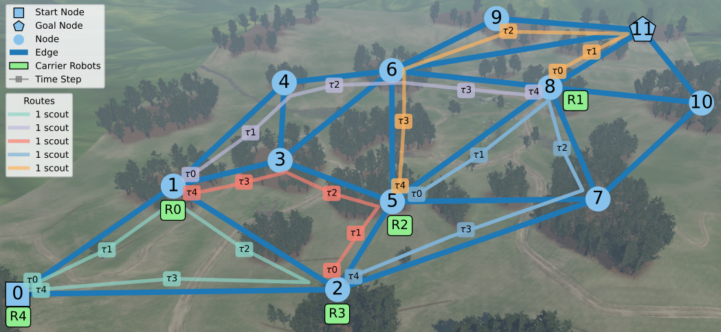
Figure 1: An example dynamical topological graph in a meadow environment with uncertain edge weights applied to a reconnaissance test scenario. The routes through the graph show the paths of scout agents deployed from carrier vehicles to explore the environment.

II RELATED WORK

Multi-robot planning on graph representations has been studied in [1] and [2]. This work investigates planning under uncertainty, which can be most generally formulated as a Partially Observable Markov Decision Process (POMDP). Many researchers have analyzed POMDPs and proposed simplifying assumptions, heuristics, and sub-problems.

II-A General Methods

The authors of [3] express a Mixed-Integer Linear Programming (MILP) formulation for a lower bound on a POMDP with perfect-recall and introduce decomposable POMDPs. However, this approach requires repeatedly solving independent linear approximations rather than solving the problem end-to-end. Other research in decomposable MDPs, as in [4], have shown success solving an infinite horizon approach in finite horizons, which is a motivational baseline to our approach of continuously replanning in evolving conditions.

There has been research toward casting partially observable control problems as fully observable underactuated stochastic control problems in belief space [5], allowing standard planning and control techniques to be applied. However, these approaches must make assumptions about the future observations value, which we avoid in our approach.

II-B Machine Learning

Machine learning approaches have been applied to capture the stochasticity in graphs. For example, a Stochastic Graph Neural Network (SGNN) has been proposed in [6] to account for random network changes due to link losses (i.e., stochasticity to the graph shape). Our approach inherently handles changes in the shape of the graph due to continuously replanning, and more specifically analyzes stochasticity in the edge weights.

In [7], the authors investigate using graph convolutional neural networks for estimating stochastic edge weights across large graphs. In contrast, our approach emphasizes planning with uncertainty and minimizing its effect, rather than estimating values.

II-C Stochastic Shortest Path Problem

Stochastic graph-based methods for analyzing POMDPs often examine the Stochastic Shortest Path Problem (SSPP). In [8], the authors consider four objective functions to measure risk applied to the SSPP. There are two common variants of the Stochastic Shortest Path Problem (SSPP) [9]: edge weights modeled as random variables as in [10], or decisions at a node resulting in probability distributions on successor edges or a single following edge as in [11]. The work proposed herein, as well as [9], considers the first case. The authors of [9] present algorithms for value iteration of POMDPs and formulating the problem as a MILP, though encounter long solve times. In this work, we formulate our model compactly, as shown in [1], which enables overcoming the common model size limitations of MILP.

The author in [10] explores analytical approaches to finding optimal paths in graphs with stochastic or multidimensional edge weights. Stochastic dynamic programming approaches have been proposed, though suffer from the curse of dimensionality when including uncertainty in the reward since probability functions would need to be discretized, as mentioned in [10].

In the work proposed herein we utilize an approach based on the Hurwicz criteria [12, 10, 13]. Hurwicz criteria was developed for decision making under uncertainty to balance pessimism and optimism by taking into consideration both the best and worst possible outcomes [14]. We define a “coefficient of optimism,” $\beta\in[0,1]$, that is set based on the tolerance of the outcome. Then for a condition $c$ that we want to minimize, which is bounded such that $c^{\llcorner}\leq c\leq c^{\ulcorner}$, the Hurwicz criteria is as follows.

$$\beta c^{\llcorner}+(1-\beta)c^{\ulcorner}$$ (1)

Thus for $\beta=1$, this criteria expresses complete optimism and for $\beta=0$, this criteria expresses complete pessimism.

III PROBLEM STATEMENT

To explore the challenges associated with heterogeneous multi-robot planning under uncertainty, we consider the problem of a team robots attempting to navigate through a region while avoiding detection. In [1], we considered a similar problem, which was addressed by introducing the notion of a dynamic topological graph– a graph where the edge weights vary with the state of the robot team on the graph. Using mixed-integer programming, we were able to demonstrate coordinated behaviors for homogeneous robot teams in deterministic environments.

In this paper, we employ a similar algorithmic approach, but consider the case where positions of observers may be unknown a priori and where fast reconnaissance robots are available for information gathering. More precisely, we introduce the following constructs:

1. Scout teammates: Support team members that move at an accelerated pace to investigate areas ahead of the rest of the team.

2. Uncertain edge costs: Costs represented as discrete random variables with uncertainty that decreases to zero when the edge cost is observed by a scout. These costs increase over time to reflect a changing observer state.

In this scenario, not only do the edge weights of the dynamic topological graph vary with the state of the robot team, but also with the state of the observers in the environment.

Ultimately our robot team is composed of two types of agents: carrier robots that are performing the underlying task (navigating to a particular location or set of locations) and scouts that can collect information to minimize uncertainty about the graph edges without incurring signficant cost. The carrier robots each hold one scout. Scouts deploy from a carrier robot and then return back to any empty carrier robot. When on board the carrier robots, scouts can charge and report their findings. The scout robots could be ground or aerial vehicles depending on the requirements of the scenario and this may affect their speed, cost of launching (UAVs may be louder, and thus more detectable), and potentially connectivity of the graph (based on the platforms capabilities). In this evaluation, we consider a general scout robot that operates on the same edges as the rest of the team and moves at an accelerated pace. Scouts can deploy when the carrier robots are at nodes (i.e., regions of cover) and return within one time step.

IV MIXED-INTEGER PROGRAMMING APPROACH

We list the parameters used in our formulation of the multi-robot reconnaissance problem in Table I and the categories of decision variables in Table II as well as their type (integer, binary, or continuous), bounds (lower (LB) and upper (UB)), and descriptions. These tables are expanded from the tables in [1] to address the new challenges of heterogenous teams and uncertainty. For clarity, we introduce parameters $n_{K}$, $n_{\tau}$, $\tau$, $\zeta$, $\eta_{v}$, and the Uncertainty category. The decision variables are divided by a horizontal line between the original decision variables and the new additions.

Our total number of robots is $n_{A}+n_{K}$, carriers and scouts. To represent the accelerated speed of the scouts, they operate with time step $\tau$. During one time step $t$ there are $n_{\tau}$ scout time steps $\tau$.

To optimize solve time we formulate out cost functions and constraints to be linear, ultimately yielding a Mixed Integer Linear Program (MILP).

TABLE I: MIP Parameters

Category	Var	Description
Problem Size	$n_{A}$	Number of carrier agents/robots
	$n_{T}$	Number of time steps in the time horizon
	$n_{E}$	Number of edges, both directions
	$n_{V}$	Number of nodes/vertices
	$n_{L}$	Number of locations ($n_{E}+n_{V}$)
	$n_{S}$	Number of start locations
	$n_{G}$	Number of goal locations
	$n_{K}$	Number of scouts
	$n_{\tau}$	Number of time steps in the time horizon
Scenario Variables	$E$	Set of edges $e$
	$V$	Set of nodes/vertices $v$
	$L$	Set of locations $l$ consisting of edges and vertices, $E\cup V$
	$S$	Set of start locations $s$, $S\subseteq L$
	$G$	Set of goal locations $g$, $G\subseteq L$
Problem Parameters	$t$	Time step from $1$ to $n_{T}$
	$\tau$	Scout time step from $1$ to $n_{\tau}$
	$n_{s}$	Number of robots at start location $s\in S$
	$n_{g}$	Number of robots at goal location $g\in G$
Cost of Traversing	$\bar{w}_{e}$	Expected cost to traverse edge $e\in E$
	$r_{e}$	Cost reduction on $e$ for teaming
	$\zeta$	Scout edge cost reduction
	$\eta_{v}$	Cost of scout launch from node $v\in V$
Uncertainty	$u_{e}^{\llcorner}$	Lower bound on uncertainty of edge $e\in E$
	$u_{e}^{\ulcorner}$	Upper bound on uncertainty of edge $e\in E$
	$\xi$	Scale of uncertainty for all edges vs traversed edges
	$\lambda$	Number of time steps for uncertainty information to decay
	$\beta$	Coefficient of optimism

TABLE II: MIP Decision Variables (At Time $t$)

Var	Type	LB	UB	Description
$p_{l,t}$	Int	0	$n_{A}$	Number of robots at location $l$
$\phi_{e,t}$	Bin	0	1	Whether robots are on edge $e$
$\psi_{t}$	Bin	0	1	Whether robots have moved
$q_{l,\tau,t^{\prime}}$	Int	0	$n_{K}$	Number of scouts at $l$ at time $\tau$
$\theta_{e^{\prime},t^{\prime}}$	Bin	0	1	Whether scouts are on $e^{\prime}$ at time $\tau$
$f_{v,t^{\prime}}$	Int	0	$n_{K}$	Number of scouts deployed from $v$
$\delta_{e^{\prime},t^{\prime}}$	Bin	0	1	Whether edge $e^{\prime}$ has been detected
$z_{e^{\prime},t}$	Cont.	0	1	Detection ratio for edge $e^{\prime}$
$C_{U_{A_{e,t}}}$	Cont.	0	$\infty$	Carrier cost of uncertainty for $e$
$C_{U_{K_{e^{\prime},t^{\prime}}}}$	Cont.	0	$\infty$	Scout cost of uncertainty for $e^{\prime}$

For an undirected graph, which we present examples of in this work, we consider both directions of each edge in the set of edges $E$. When considering the uncertainty on an edge, the uncertainty is the same for both directions on the edge and thus detecting an edge in one direction is equivalent to detecting the edge in the other direction. Additionally, decision variables pertaining to scouts exclude the last time step $t=n_{T}$ and potentially the first time step if they are restricted from launching. Overall these factors reduce the number of variables necessary. We denote these cases by specifying $e^{\prime}\in E^{\prime}$, where $E^{\prime}$ is the set of one direction of all edges, and $t^{\prime}$ in Table II. To reduce complexity, we drop this notation in our derivation.

IV-A Scout and Uncertainty Cost Functions

IV-A1 Cost of Uncertainty

We first consider a risk-aware cost of traversing edge $e$, $\tilde{C}_{W_{e,t}}$, which is a linear cost that depends on the weight on the edge, $w_{e}$. This cost applies to the carrier robots if they use that edge at time $t$ (i.e., $\phi_{e,t}$) and we add a term for each scout that uses that edge at scout time step $\tau$ and overall time step $t$ (i.e., $q_{e,\tau,t}$) with the cost reduced by $\zeta$ to represent the lower cost for scout’s to traverse.

$$\tilde{C}_{W_{e,t}} =w_{e}\bigg{(}\phi_{e,t}+\zeta\sum_{\tau=1}^{n_{\tau}}q_{e,\tau,t}\bigg{)}$$ (2)

We consider $w_{e}$ to be a random variable with an expected value of $\bar{w}_{e}$ and associated uncertainty (e.g., a 95% confidence interval on a Gaussian distribution). The upper bound of $w_{e}$ is $\bar{w}_{e}+u_{e}^{\ulcorner}$ and the lower bound is $\bar{w}_{e}-u_{e}^{\llcorner}$. We then apply the Hurwicz criteria from (1) to represent $w_{e}$ as follows.

$$w_{e} \approx\beta(\bar{w}_{e}-u_{e}^{\llcorner})+(1-\beta)(\bar{w}_{e}+u_{e}^{\ulcorner})$$ (3)

This results in $\bar{w}_{e}$ plus an expression of the uncertainty which we call $u_{e}=(1-\beta)u_{e}^{\ulcorner}-\beta u_{e}^{\llcorner}$. We can then use this formulation of $w_{e}$ in our expression of the simplified cost of traversing from (2).

$$\tilde{C}_{W_{e,t}} =\bar{w}_{e}\bigg{(}\phi_{e,t}+\zeta\sum_{\tau=1}^{n_{\tau}}q_{e,\tau,t}\bigg{)}+u_{e}\bigg{(}\phi_{e,t}+\zeta\sum_{\tau=1}^{n_{\tau}}q_{e,\tau,t}\bigg{)}$$ (4)

The first term in (4) is the expected cost of traversing. The second term in (4) is the impact of the uncertainty on the cost of traversing and we label this term $C_{U_{W_{e,t}}}$.

We then formulate our total cost of uncertainty from the uncertainty of traversed edges, $C_{U_{W_{e,t}}}$, and the uncertainty on all edges. We consider the uncertainty across the graph to encourage general exploration, and scale it by $\xi$ to reflect the priority of general exploration versus exploration on the edges that are planned to be used. This expression is as follows and represents the maximum cost of uncertainty.

$$u_{e}\bigg{(}\xi+\phi_{e,t}+\zeta\sum_{\tau=1}^{n_{\tau}}q_{e,\tau,t}\bigg{)}$$ (5)

The role of the scouts in our formulation is to explore uncertain edges ahead of the rest of the team to reduce uncertainty. To reflect this, we add a ratio $z_{e,t}$ for how recently an edge has been detected and use that to reduce the uncertainty of explored edges. This ratio $z_{e,t}$ is $0$ if an edge has not yet been detected and $1$ when an edge was detected at $t-1$, and this value decays over time to reflect how recently an edge has been explored by the scouts. When running with a receding horizon, the weights and uncertainty on the edges would then be updated based on new data from the scouts as well.

At a time step $t$, after scouts explore an edge, they no longer have the cost of uncertainty on additional passes, thus we only consider uncertainty on their first pass on an edge by tracking where scouts use an edge $e$ at time $t$ with decision variables $\theta_{e,t}$. We combine these notions with the expression in (5) to calculate our overall cost of uncertainty for a particular edge $e$ at time $t$.

$$C_{U_{e,t}}=u_{e}(\xi(1-z_{e,t})+(\phi_{e,t}+\zeta\theta_{e,t})(1-z_{e,t}))$$ (6)

The expression in (6) is nonlinear. To keep our cost and constraints linear, we break this expression into a linear component and two cost constraints as follows.

$$C_{U_{e,t}} =u_{e}\xi(1-z_{e,t})+C_{U_{A_{e,t}}}+C_{U_{K_{e,t}}}$$ (7)

$$C_{U_{A_{e,t}}} \geq u_{e}(\phi_{e,t}-z_{e,t})$$ (8)

$$C_{U_{K_{e,t}}} \geq\zeta u_{e}(\theta_{e,t}-z_{e,t})$$ (9)

Constraints (8) and (9) assume $u_{e}\geq 0$. In our test case we aim to be risk adverse, so we can assume $u_{e}^{\llcorner}<u_{e}^{\ulcorner}$ and $\beta<0.5$ to assure $u_{e}\geq 0$. In other scenarios, we would add additional constraints to remove these assumptions.

When an edge is not traversed by the carrier robots (i.e., $\phi_{e,t}=0$) the cost of uncertainty from the carrier robots using that edge, $C_{U_{A_{e,t}}}$, should be zero. In this case, the constraint in (8) would be a negative bound, but the overall bound on $C_{U_{A_{e,t}}}\geq 0$, as stated in Table II, would set the value of $C_{U_{A_{e,t}}}$ to $0$ since we’re minimizing cost. When the edge is traversed, (8) is positive and thus is the value of $C_{U_{A_{e,t}}}$ since we are minimizing cost. These properties are the same for $C_{U_{K_{e,t}}}$ in (9).

IV-A2 Cost of Traversing

From our expression for the risk-aware cost of traversing in (4), the uncertainty component is captured with $C_{U_{e,t}}$ so we can separately express the component for the expected cost of traversing. Additionally, we add a linear cost reduction based on the number of agents on an edge to incentivize teaming, as in [1].

$$C_{W_{e,t}} =\bar{w}_{e}\phi_{e,t}-r_{e}p_{e,t}+\zeta\bar{w}_{e}\sum_{\tau=1}^{n_{\tau}}q_{e,\tau,t}$$ (10)

IV-A3 Cost of Launch

To represent the risk associated with deploying a scout vehicle, in particular an aerial vehicle which may be noticeable and noisy, we introduce a cost associated with launching the vehicle. The launch cost for a particular vertex, $\eta_{v}$, is the average cost of the surrounding edges multiplied by a scaling factor (for how much to weight the launch cost compared to the edge cost). For all $t$ and $v$, we express the cost of launching, $C_{F_{v,t}}$.

$$C_{F_{v,t}}=\eta_{v}f_{v,t}$$ (11)

IV-A4 Cost of Time

We use the cost of time as derived in [1] using decision variables $\psi_{t}$ to track movement on the graph.

$$C_{T}=\sum_{t=1}^{n_{T}}t\psi_{t}$$ (12)

IV-A5 Total Cost

We combine our cost expressions from (7), (10), (11), and (12) into our overall objective function.

$$C=C_{T}+\sum_{t=1}^{n_{T}}\bigg{(} \sum_{e\in E}\big{(}C_{W_{e,t}}+C_{U_{e,t}}\big{)}+\sum\limits_{v\in V}C_{F_{v,t}}\bigg{)}$$ (13)

Each of these terms can be scaled based on the priorities of a scenario.

IV-B Scout and Uncertainty Constraints

We add the following constraints when expanding our MIP formulation from [1] for scouts and incorporating uncertainty.

IV-B1 Time Tracking Variables

We extend the time tracking variables $\psi_{t}$ from [1] to track carrier robots and scouts moving on edges for each time step.

$$\psi_{t}\geq\frac{1}{n_{A}+n_{K}n_{\tau}}\sum_{e\in E}\bigg{(}p_{e,t}+\sum_{\tau=1}^{n_{\tau}}q_{e,\tau,t}\bigg{)}$$ (14)

IV-B2 Scout Edge Used Variables

We set the binary variable $\theta_{e,t}$ to $1$ if there are scouts on edge $e$ during any scout time $\tau$ and overall time $t$ and $0$ otherwise with the following constraint. This constraint assumes $\theta_{e,t}$ contributes to increasing the cost function, such that it will only be set to $1$ when required by the inequality.

$$\theta_{e,t}\geq\frac{1}{n_{K}n_{\tau}}\sum_{\tau=1}^{n_{\tau}}q_{e,\tau,t}$$ (15)

IV-B3 Scout Deployment Constraints

We consider the scouts to be linked to carrier robots such that scouts must launch from a carrier and return to carrier without a scout. We use decision variables $f_{v,t}$ to track the number of scouts deployed from a particular location $v$ at time step $t$. We bound this value based on the number of carrier robots at that location. Additionally, we add start and goal constraints to deploy and return to those locations. For all $t$ and $v$, we add the following constraints.

$$f_{v,t}\leq p_{v,t},\quad q_{v,1,t}=f_{v,t},\quad q_{v,n_{\tau},t}=f_{v,t}$$ (16)

IV-B4 Maximum Scouts

We constrain the maximum number of scouts across all locations at a particular $\tau$ and $t$ to be equal to the number of scouts deployed.

$$\sum_{l\in L}q_{l,\tau,t}=\sum_{v\in V}f_{v,t}$$ (17)

IV-B5 Scout Sequential Constraints

To restrict the scouts movement to the topological graph, for each node $v_{j}$, we constrain the number of robots entering the node and in node to be equal to the number of robots in the node and leaving the node in the next time step. Thus, for all $t$, $\tau\in[2,n_{\tau}]$ and node $v_{j}$, we add the following constraint.

$$\sum_{\begin{subarray}{c}l_{ij}=(v_{i},v_{j})\in L\end{subarray}}q_{l_{ij},\tau-1,t}=\sum_{\begin{subarray}{c}l_{ji}=(v_{j},v_{i})\in L\end{subarray}}q_{l_{ji},\tau,t}$$ (18)

IV-B6 Edge Detection Variables

We add constraints for variables to track which edges have been detected by the traversal of a scout. For $e$, $t=[1,n_{T}-2]$, $\delta_{e,t}$ tracks if edge $e$ has been detected at time $t$.

$$\delta_{e,t}\leq\sum_{\begin{subarray}{c}\tau=1\end{subarray}}^{n_{\tau}}{q_{e,\tau,t}}$$ (19)

We use $z_{e,t}$ to track the horizon of the detection. If edge $e$ was detected in the last time step then $z_{e,t}$ is equal to 1, then over time $z_{e,t}$ will decay reflecting the increasing uncertainty since the last time the edge was detected. If edge $e$ was only detected in the current time step $t$ then $z_{e,t}=0$, but $z_{e,t+1}$ will be 1. For $e$ and $t$, we add the following constraint.

$$z_{e,t}\leq\sum_{t_{h}=\max{(t-\lambda,1)}}^{t-1}\delta_{e,t_{h}}\frac{\lambda-(t-t_{h})+1}{\lambda(t-t_{h})}$$ (20)

IV-C Uncertainty-Aware Multi-Robot Optimization Problem

We combine our newly defined objective functions and constraints with the original costs and constraints from [1] to form our overall MIP in Table III. In this table, equation numbers starting with “[1]-” represent equation numbers from [1], reproduced here for completeness. These include general constraints for setting support variables used in our cost functions and constraints to restrict movement to the topological graph. For the formulation of these constraints and further detail, please refer to [1]. In this formulation, we captured our costs and constraints linearly and used mixed-integer linear programming to solve our problem with the Gurobi optimizer [15].

TABLE III: MIP Optimization Problem with Uncertainty and Scouts

Optimization Problem			Eq.
$\min~{}C_{T}+\sum\limits_{t=1}^{n_{T}}\bigg{(}\sum\limits_{e\in E}\big{(}C_{W_{e,t}}+C_{U_{e,t}}\big{)}+\sum\limits_{v\in V}C_{F_{v,t}}\bigg{)}$ s.t.			(13)
Scout and Uncertainty Constraints	$C_{U_{A_{e,t}}}\geq u_{e}(\phi_{e,t}-z_{e,t}),$	$\forall e,t$	(8)
	$C_{U_{K_{e,t}}}\geq u_{e}(\theta_{e,t}-z_{e,t}),$	$\forall e,t$	(9)
	$\theta_{e,t}\geq\frac{1}{n_{K}n_{\tau}}\sum\limits_{\tau=1}^{n_{\tau}}q_{e,\tau,t},$	$\forall e,t$	(15)
	$f_{v,t}\leq p_{v,t},\quad q_{v,1,t}=f_{v,t},\quad q_{v,n_{\tau},t}=f_{v,t},$	$\forall v,t$	(16)
	$\sum_{l\in L}q_{l,\tau,t}=\sum_{v\in V}f_{v,t},$	$\forall\tau,t$	(17)
	$\sum\limits_{\begin{subarray}{c}l_{ij}=(v_{i},v_{j})\in L\end{subarray}}q_{l_{ij},\tau-1,t}=\sum\limits_{\begin{subarray}{c}l_{ji}=(v_{j},v_{i})\in L\end{subarray}}q_{l_{ji},\tau,t},$	$\forall t,v_{j},\newline \tau\in[2,n_{\tau}]$	(18)
	$\delta_{e,t}\leq\sum_{\begin{subarray}{c}\tau=1\end{subarray}}^{n_{\tau}}{q_{e,\tau,t}},$	$\forall e,t=[1,n_{T}-2]$	(19)
	$z_{e,t}\leq\sum_{t_{h}=\max{(t-\lambda,1)}}^{t-1}\delta_{e,t_{h}}\frac{\lambda-(t-t_{h})+1}{\lambda(t-t_{h})},$	$\forall e,t$	(20)
Carrier Robot Constraints	$\psi_{t}\geq\frac{1}{n_{A}+n_{K}n_{\tau}}\sum\limits_{e\in E}\bigg{(}p_{e,t}+\sum\limits_{\tau=1}^{n_{\tau}}q_{e,\tau,t}\bigg{)},$	$\forall t$	(14)
	$\phi_{e,t}\geq\frac{1}{n_{A}}p_{e,t},$	$\forall e,t$	[1]-(13)
	$p_{s,1}=n_{s},$	$\forall s$	[1]-(15)
	$p_{g,n_{T}}\geq n_{g},$	$\forall g$	[1]-(16)
	$\sum\limits_{l\in L}p_{l,t}=n_{A},$	$\forall t$	[1]-(17)
	$\sum\limits_{l_{ij}=(v_{i},v_{j})\in L}p_{l_{ij},t-1}=\sum\limits_{l_{ji}=(v_{j},v_{i})\in L}p_{l_{ji},t},$	$\forall v_{j},\newline t\in[2,n_{T}]$	[1]-(18)

V COMPUTATIONAL RESULTS AND DISCUSSION

We evaluate our approach in scenarios that emphasize the benefit of uncertainty reduction using scout robots.

V-A Ablation Study

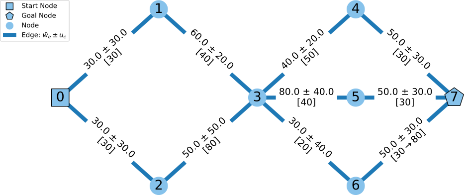
Figure 2: Example dynamic topological graph with expected edge weights, uncertainty, and the true cost labeled for each edge. The cost of edge (6,7) changes over time from 30 to 80.

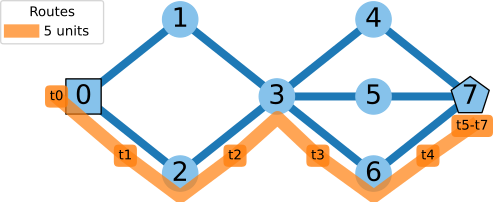
(a) Expected edge weights without uncertainty and scouts, true cost = 210

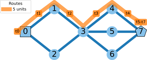
(b) Expected edge weights and uncertainty without scouts, true cost = 150

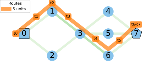
(c) Expected edge weights and uncertainty with scouts, without certainty decay, true cost = 170

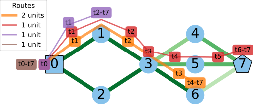
(d) Expected edge weights and uncertainty with scouts and certainty decay, true cost = 140

Figure 3: Ablation study illustrating the advantages of considering uncertainty, scouts for the reduction of uncertainty, and certainty decay for evolving conditions. Each plot shows the final paths of the robot units through the path. Each unit is composed of a robot carrier and scout. The first case is the baseline from [1] and each subsequent case adds one of the components from the algorithm proposed in this paper to show the resulting effect to the final team routes through the graph. In the two cases that include scout robot deployments the darkness of the edges reflect the number of time steps the scouts explored that edge.

To demonstrate the advantages of each component of our algorithm, we performed an ablation study on the example graph in Fig. 2. For clarity, we consider symmetric uncertainty about an expected value for an edge weight, as denoted in Fig. 2 where the true values of the edge weights are shown in brackets. These values can be recovered by the scouts traversing the corresponding edges. As time progresses the “true” value will evolve so frequent exploration will yield updated values. To represent this, on edge (6,7) the true cost starts at 30, but goes to 80 at later time steps. This could be due to an observer moving to more easily view (6,7). In this example, all robot units (carrier robots with scouts) start at node 0 and the overall goal is for some subset of units to reach node 7 within 8 time steps $t$. Scouts can move 8 scout time steps, $\tau$, within one overall time step, $t$, (i.e., 8 times faster than carrier robots). Their movement costs a quarter of the cost of an edge (weight and uncertainty) since they would be less detectable. Scouts can launch at all time steps except for the last, since there is no value to the information gathered once the team has reached the goal.

We consider four cases in our ablation study in Fig. 3:

1. Expected edge weights alone, as implemented in [1]

2. Expected edge weights with uncertainty (i.e., including cost (7) and cost constraint (8), excluding scout terms)

3. Uncertain edge weights with the ability to deploy scouts to reduce the uncertainty to zero (i.e., (20) is modified to sum $\delta_{e,t_{h}}$ without any $\lambda$ term)

4. Uncertain edge weights with the ability to deploy scouts with decay on the certainty gained from the scouts actions, as influenced by (20)

Each of these scenarios is solved for using our optimization problem, in Table III, with the corresponding components removed from the algorithm. The resulting final team paths for each are shown in Fig. 3, as well as the true cost for the route to the goal node. For simplicity, we use a coefficient of optimism, $\beta$, of 0 to find solutions that are most risk adverse.

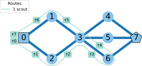
(a) Scout routes at t = 0

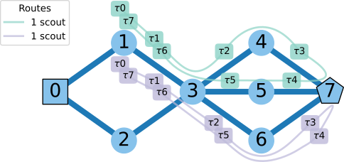
(b) Scout routes at t = 2

Figure 4: Routes of the scout agents when deployed in the ablation case c. Full team routes are shown in Fig. c.

In Fig. 3(a), case a, the path with minimum expected edge cost is selected. However, this path has very high uncertainty, so the resulting true cost is significantly higher than expected. When the uncertainty is considered in Fig. 3(b), case b, a path that minimizes the expected weights plus the maximum uncertainty is found. This plans for a worst case scenario, but the resulting true cost is less than the expected cost. In Fig. 3(c), case c, scouts are deployed at node 0 and then again at node 1 in order to reduce the uncertainty in planning. The scout paths are shown in Fig. 4. These deployments result in a more informed route, however conditions are continuously evolving, and exploring once is not sufficient to see the future cost increase associated with traversing edge (6,7). Finally, we introduce decaying certainty to our algorithm in case d, such that uncertainty increases after a scout visit to incentivize revisiting locations to update edge weight observations. This yields a final path to the goal node in Fig. 3(d) that minimizes the true cost. Here we see robots stay behind at nodes to be able to deploy scouts to reduce the overall uncertainty; these routes look similar to those in Fig. 4.

V-B Coefficient of Optimism

Our coefficient of optimism $\beta$ from the Hurwicz criteria, as employed in (3), reflects our tolerance of risk. The most risk adverse approach is setting $\beta=0$ such that we consider the uncertainty in the worst case scenario. This results in scouts exploring more to gather more information and reduce the overall risk. Fig. 5 shows the number of time steps scouts explore each edge for various $\beta$ values. $\beta$ could be set based on the operational scenario and tolerance for risk.

V-C Combinatorial Considerations and Computation Time

We investigated how the algorithm from [1] scales for considering uncertainty and adding a new class of vehicles, scouts. Our total number of decision variables scales as $n_{T}(1+n_{L}+n_{E}+\mathbf{n_{L}n_{\bm{\tau}}+5n_{E}+n_{V}})$. Here we have indicated the additions from the algorithm in [1] in bold. The greatest impact comes from considering the time step of the scouts, $\tau$, to occur within each time step of the carrier robots, $t$, which adds $n_{T}n_{L}n_{\tau}$ variables to capture full scout trajectories at each $t$. Ultimately, we were able to leverage the key innovation in [1] to formulate the problem such that the number of robots is removed from our decision space to keep the solve time tractable for larger graph sizes.

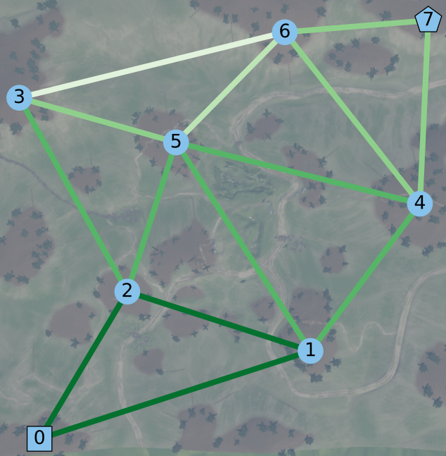
(a) $\beta=0$

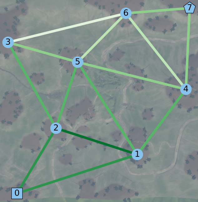
(b) $\beta=0.15$

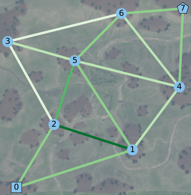
(c) $\beta=0.30$

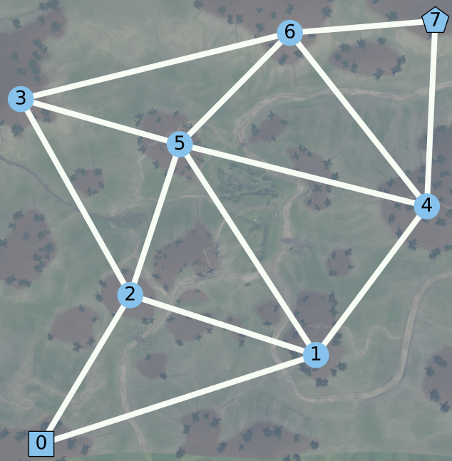
(d) $\beta=0.45$

Figure 5: Scout exploration of each edge for different coefficients of optimism, $\beta$.

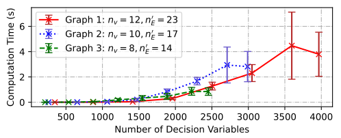
Figure 6: Computation time for three example graphs of varying sizes versus the number of decision variables. Error bars are one standard deviation.

To adjust for new information and an evolving environment, we plan in a receding horizon. To demonstrate the scaling of our approach, in Fig. 6 we plot the computation time for each iteration on three differently sized graphs versus the number of decision variables. Graph 1 is shown in Fig. 4 and Graph 3 is shown in Fig. 5. When planning through an environment, the data points in Fig. 6 occur right to left, with the total number of decision variables decreasing with the receeding horizon. These computation times come from averaging across 100 trials using the Gurobi optimizer [15] on an Intel® Core™ i7-10875H CPU @ 2.30GHz × 16. The longest computation time remains on the order of seconds, which enables regular re-planning.

VI CONCLUSION

In this paper, we explored multi-robot planning on dynamic topological graphs using mixed-integer programming for two challenging cases: heterogeneous teams and planning under uncertainty. We use the uncertainty in our problem as a motivation for a heterogeneous team, introducing scout robots that can investigate the environment to collect data and reduce the uncertainty of future team actions. Our approach results in a MILP that can be solved rapidly with a receding horizon in real-world scenarios. We test this approach in example scenarios and demonstrate the ability to successfully generate risk-aware plans for multi-robot teams.

References

- [1] C. A. Dimmig, K. C. Wolfe, and J. Moore, “Multi-robot planning on dynamic topological graphs using mixed-integer programming,” arXiv preprint arXiv:2303.11966, 2023.
- [2] S. Oughourli, M. Limbu, Z. Hu, X. Wang, X. Xiao, and D. Shishika, “Team coordination on graphs with state-dependent edge cost,” arXiv preprint arXiv:2303.11457, 2023.
- [3] V. Cohen and A. Parmentier, “Linear programming for decision processes with partial information,” arXiv preprint arXiv:1811.08880, 2018.
- [4] D. Bertsimas and V. V. Mišić, “Decomposable markov decision processes: A fluid optimization approach,” Operations Research, vol. 64, no. 6, pp. 1537–1555, 2016. [Online]. Available: https://doi.org/10.1287/opre.2016.1531
- [5] R. Platt Jr, R. Tedrake, L. Kaelbling, and T. Lozano-Perez, “Belief space planning assuming maximum likelihood observations,” 2010.
- [6] Z. Gao, E. Isufi, and A. Ribeiro, “Stochastic graph neural networks,” IEEE Transactions on Signal Processing, vol. 69, pp. 4428–4443, 2021.
- [7] J. Hu, C. Guo, B. Yang, and C. S. Jensen, “Stochastic weight completion for road networks using graph convolutional networks,” in 2019 IEEE 35th International Conference on Data Engineering (ICDE), April 2019, pp. 1274–1285.
- [8] J. D. Jordan and S. Uryasev, “Shortest path network problems with stochastic arc weights,” Optimization Letters, vol. 15, no. 8, pp. 2793–2812, Nov 2021. [Online]. Available: https://doi.org/10.1007/s11590-021-01712-5
- [9] P. Buchholz and I. Dohndorf, “Optimal decisions in stochastic graphs with uncorrelated and correlated edge weights,” Computers & Operations Research, vol. 150, p. 106085, 2023. [Online]. Available: https://www.sciencedirect.com/science/article/pii/S030505482200315X
- [10] R. P. Loui, “Optimal paths in graphs with stochastic or multidimensional weights,” Commun. ACM, vol. 26, no. 9, p. 670–676, sep 1983. [Online]. Available: https://doi.org/10.1145/358172.358406
- [11] D. P. Bertsekas and J. N. Tsitsiklis, “An analysis of stochastic shortest path problems,” Mathematics of Operations Research, vol. 16, no. 3, pp. 580–595, 1991. [Online]. Available: https://doi.org/10.1287/moor.16.3.580
- [12] L. Hurwicz, “The generalized bayes minimax principle: a criterion for decision making under uncertainty,” Cowles Comm. Discuss. Paper Stat, vol. 335, p. 1950, 1951.
- [13] T. Denœux, “Decision-making with belief functions: A review,” International Journal of Approximate Reasoning, vol. 109, pp. 87–110, 2019. [Online]. Available: https://www.sciencedirect.com/science/article/pii/S0888613X1830505X
- [14] “The hurwicz criterion.” [Online]. Available: https://www.leonidhurwicz.org/hurwicz-criterion/
- [15] Gurobi Optimization, LLC, “Gurobi Optimizer Reference Manual,” 2023. [Online]. Available: https://www.gurobi.com