MeanAP-Guided Reinforced Active Learning for Object Detection

Abstract

Active learning presents a promising avenue for training high-performance models with minimal labeled data, achieved by judiciously selecting the most informative instances to label and incorporating them into the task learner. Despite notable advancements in active learning for image recognition, metrics devised or learned to gauge the information gain of data, crucial for query strategy design, do not consistently align with task model performance metrics, such as Mean Average Precision (MeanAP) in object detection tasks. This paper introduces MeanAP-Guided Reinforced Active Learning for Object Detection (MAGRAL), a novel approach that directly utilizes the MeanAP metric of the task model to devise a sampling strategy employing a reinforcement learning-based sampling agent. Built upon LSTM architecture, the agent efficiently explores and selects subsequent training instances, and optimizes the process through policy gradient with MeanAP serving as reward. Recognizing the time-intensive nature of MeanAP computation at each step, we propose fast look-up tables to expedite agent training. We assess MAGRAL’s efficacy across popular benchmarks, PASCAL VOC and MS COCO, utilizing different backbone architectures. Empirical findings substantiate MAGRAL’s superiority over recent state-of-the-art methods, showcasing substantial performance gains. MAGRAL establishes a robust baseline for reinforced active object detection, signifying its potential in advancing the field.

1 Introduction

The pursuit of artificial intelligence has perennially revolved around two fundamental aspects: data and models. While extensive work has refined model designs, contemporary research endeavors increasingly direct their focus towards more efficient data annotation methods (such as automatic labeling [18]) and smarter data utilization paradigms. Active Learning (AL) stands out among these approaches, aiming to craft high-performance models with the sparsest possible set of labeled instances by judiciously identifying and annotating the most informative data points.

Moreover, practical AI applications often encounter a dilemma: models trained on limited labeled data struggle to perform effectively when confronted with abundant, unused, unlabeled data. The sheer volume of unlabeled data remains largely untapped due to resource constraints. In response, active learning emerges as a strategic solution, enabling the targeted annotation of the most valuable data points. This approach optimizes data use, enhancing AI system efficiency and practicality significantly.

Figure 1: An illustration of the difference between hand-crafted or learned uncertainty and model performance metric (e.g. MeanAP). The yellow sample brings the maximum entropy (uncertainty) to current labeled pool, while the green one is the most effective sample for the increase of performance. The purple circle represents the distribution active learning has learned in previous cycles.

Then, what kind of data is the most informative? It is easy to be aware of that the data complementary to the currently labeled ones in the model feature space is the most informative. And this informativeness is mainly characterized by uncertainty. Recent works [31, 1, 32, 34] have put forward some different definitions of uncertainty, developed by handcrafting or learning and used as the query strategy for active learning. Although their works have achieved some results, the uncertainty they defined is not always equal to the performance metric of task model (e.g. MeanAP). As illustrated in Figure 1, assume we have a dataset with labeled data marked by red ($+$ and $-$ represent two different categories), we intend to train a good classifier to distinguish the two classes. Then, if we use the uncertainty defined by entropy [20], we’ll choose the sample marked by yellow because it’s the one most far away from what active learning has learned (the purple ellipse in the figure). Under this circumstance, we will obtain the classifier represented by the solid line which misjudges the $+$ class data on the right. As a substitute, if we select the green sample, we’ll obtain the classifier represented by the dotted line, which achieves the best performance. The green sample corrects the knowledge of active learning model and thus is the most effective data for the task model at this step. We aim to select this kind of data.

In this paper, we propose a MeanAP-Guided Reinforced Active Learning method for Object Detection (MAGRAL), to directly leverage the MeanAP of task model to develop the sampling mechanism, enhancing the usefulness of selected images. Considering the gain of model performance ($\Delta$MeanAP) is non-differentiable about the selected samples $(\Delta x)$, which means MeanAP cannot be directly taken to optimize sampling network, we deploy a reinforcement learning (RL) based agent to guide the search, adopt the MeanAP as the reward and optimize the agent by policy gradient. In this way, the agent outputs the selected samples which achieve maximum $\Delta\text{MeanAP}/\Delta x$ directly instead of other information scores.

Furthermore, as MAGRAL is required to compute mean average precision with unlabeled sampled examples, we utilize a semi-supervised model to estimate MeanAP. Besides, considering reinforcement learning based agent is trained with reward ($\Delta\text{MeanAP}$) at each iteration which asks to train the whole semi-supervised model from scratch time and time again, the total training time of MAGRAL (including training the proxy task model for $total\_iter$ times) is intolerable. Acceleration techniques (e.g. fast lookup table) are adopted to speed up the agent training. In all, MeanAP-guided strategy sophisticatedly utilizes model performance metric to measure the data informativeness, achieves an improvement of 0.9%, 2.6% and 4.3% over existing methods MI-AOD[32], LL4AL[31] and random sampling respectively with 10k labeled data on PASCAL VOC and provides a solid baseline for reinforced active object detection.

Our contributions can be summarized as:

(1) We identified the misalignment between previous uncertainty-based or distribution-based methods and task model performance. We proposed the MeanAP-guided query strategy, enhancing the precision of AL algorithm.

(2) We devised a reinforcement learning agent for sampling, with MeanAP as the agent’s reward, addressing the non-differentiable discrete search space of MeanAP.

(3) MAGRAL algorithm surpasses state-of-the-art methods, incorporating a fast look-up table for accelerated performance.

2 Related Works

2.1 Query Strategies of Active Learning

Classical Active Learning Methods. These methods commonly utilize artificially defined metrics to measure the informativeness of unlabeled data. According to the definition of informativeness, they can be classified into uncertainty-based method, distribution-based method and their combinations.

Uncertainty is the most widely-used metric for data sampling and is implemented in several ways, such as information theoretic heuristics (e.g. entropy maximization [20]), query-by-committee [6, 9] and Bayesian models [11, 10]. Yet, the instances sampled by uncertainty methods usually have information redundancy [26], which results from not taking into account the information association among sampled instances.

Distribution-based methods have solved this problem by selecting as diverse samples as possible with the basis on mastering the distribution of unlabeled data. Core-set technique [26] has chosen the most representative samples by minimizing the distance from all unsampled points to sampled points in the feature space, and has been proven to be effective in large-scale classification tasks. And [14] has utilized hand-crafted context-aware similarity metric to select instances that best represent the global data distribution. However, these manually designed distance-based methods perform poor on high-dimensional data [7].

As a compromise, some methods combine uncertainty and representativeness metrics to improve AL performance by exploration-exploitation trade-offs [25], combination of entropy and information density [20], or ensemble of models [19, 29], but cannot coordinate them well.

Deep Learning Based Active Learning Methods. In the deep learning era, new strategies have been proposed to directly learn the informativeness of unlabeled data [31] or directly select samples [28] through neural network, replacing previous hand-crafted strategies. The learning loss method [31] has utilized the predicted ”loss” to estimate sample uncertainty. And the VAAL method [28] has deployed an adversarial mechanism to learn image uncertainty and representation at the same time.

However, all these learned metrics are still weakly correlated to the task model performance, and cannot accurately reflect the contributions of selected samples to the performance. Our MAGRAL method directly utilizes this performance as metric of query strategy and solves the problem.

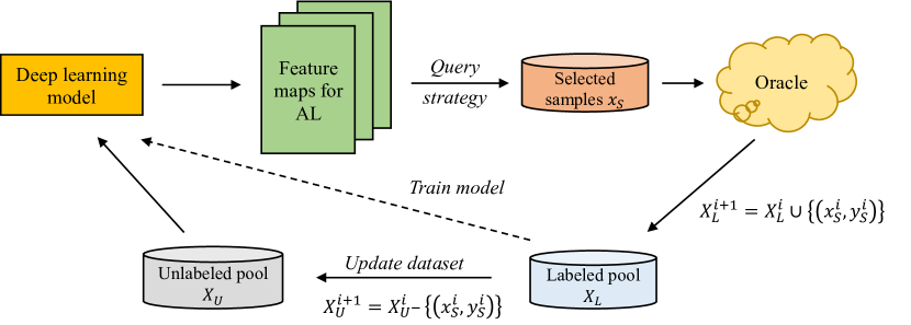
(a) Classical Active Learning Pipeline.

(b) MAGRAL Pipeline.

Figure 2: (a) An example of classical pool-based deep active learning. The solid line represents the active learning data flow, while the dotted line represents the deep model training data flow. (b) An overview of MeanAP-guided Reinforced Active Learning for Object Detection (MAGRAL). The part outlined by the dash-dot line is the agent training part, which aims to obtain a sampling agent that can reflect the effectiveness of samples in the unlabeled pool and output the selected samples $x_{s}$.

2.2 Deep Reinforcement Active Learning

Reinforcement learning has been introduced to learn a better query strategy by maximizing the task model performance. [3] has put forward a policy gradient based method to jointly learn data representation, selection heuristics and model prediction function. [23] has proposed a imitation learning based query strategy for NLP tasks. Moreover, in order to better consider representativeness of unlabeled data, [5] has leveraged a bi-directional RNN to sample all instances in one step for one shot learning. Recent works [17, 4] have suggested using Deep Q-Network to learn sampling strategy for pool-based AL.

However, they cannot be applied to object detection task, because their reward is unable to integrate the uncertainty of multi-instances in a single image. Our method subtly avoids this problem by taking $\Delta\text{MeanAP}$ as the reward, and reflects the performance of detector directly.

2.3 Active Learning for Object Detection

Few of existing AL works focus on object detection which faces complex instance distributions in a single image and is difficult to define an uncertainty metric or RL reward term.

LL4AL [31] originally for classification can easily migrate to object detection by using loss predictions of instances instead of images. [2] has proposed to estimate the informativeness through combining the uncertainty of foreground objects (for classification) and background pixels (for localization). On this basis, CDAL [1] has introduced spatial context to select most representative samples according to the distances between features of unlabeled and labeled data.

Furthermore, recent work MI-AOD [32] has raised to use a pair of adversarial classifier and the detection network to learn the image uncertainty and query strategy, different from previous instance-/pixel- level feature based methods [33, 34]. And MI-AOD implicitly leverages semi-supervised mechanism to enhance the model performance on the basis of similar data setting between AL and semi-supervised learning. However, these methods use indirect metrics as before, which harms the detection model performance. We put forward a new idea to utilize the performance metric MeanAP directly to guide the selection process and achieve a high performance.

3 Technical Approach

3.1 Problem Definition

Active learning for object detection follows the setting that a small labeled set $X_{L}$ containing images with instance labels, denoted as $(x_{L},y_{L})$ and a large unlabeled set $X_{U}$ without labels, denoted as $(x_{U})$ are given. The labels include locations of bounding boxes and their corresponding categories.

For each cycle, a detection model $M_{i}$ ($i$ denotes the cycle subscript) is firstly trained with the labeled set $X_{L}^{i}$. Next, active learning selects a set of images $x_{S}^{i}$ from the unlabeled set $X_{U}^{i}$ by query strategy, annotates them and merges them with $X_{L}^{i}$ to form a new labeled set $X_{L}^{i+1}$. We can formulate it as $X_{L}^{i+1}=X_{L}^{i}\cup(x_{S}^{i},y_{S}^{i})$. After that, the new labeled set $X_{L}^{i+1}$ is used to train the detection model $M_{i+1}$. Active learning repeats this process until the labeled set size reaches the budget $B$. A typical active learning pipeline is shown in Figure 2(a). We expect the selected images $x_{S}^{i}$ improve the model performance most significantly at cycle $i$.

Therefore, the design of query strategy is crucial to active learning which inspires our proposed method.

3.2 Overview

Our proposed method is named after MeanAP-Guided Reinforced Active Learning for Object Detection (MAGRAL), which derives its query strategy by utilizing the performance of task learner, to maximize the impact of selected samples.

As shown in Figure 2(b), the pipeline of MAGRAL is similar to that of typical pool-based method. However, our method has employed a sampling agent (controller) to function as the query strategy on the basis of reinforcement learning (RL). With the controller, the difficulty that the performance metric MeanAP is discrete about the search space is skillfully solved. Furthermore, the part framed by dash-dot line is the training module of sampling controller, and is inserted into the whole AL pipeline as the query strategy. The other parts function the same as classical AL.

We then briefly illustrate the workflow of our algorithm. As shown in Figure 2(b), firstly, we have two data pools $X_{L}$ and $X_{U}$, and a initialized sampling controller. Then, with RL, we use these two data pools and downstream detection model to compute $\Delta\text{MeanAP}$ (reward) to train the sampling controller. As a result, the trained controller can most describe the validity of data for the downstream task. Therefore, we adopt the trained agent to select the most informative data batch as $x_{S}$ and go to next AL cycle.

In summary, MAGRAL creatively utilizes a sampling controller to function as query strategy and to achieve active learning. In the following parts, we will discuss the two most important components that make up MAGRAL framework: i) controller architecture; ii) controller training pipeline and reward calculation.

3.3 MAGRAL Controller Architecture

As shown in Figure 3, we followed the basic idea of [35] and deployed a Long Short-Term Memory networks (LSTM) [13] as sampling controller to select the most informative images from the unlabeled pool.

To cooperate with this design, MAGRAL models each image as a search unit. Suppose there is a dataset containing $N$ images in total, of which $N_{L}$ images are labeled and $N_{U}$ are not. Then, we designed the search chain of controller as $N_{U}$ units. As stated above, the basic unit of MAGRAL agent is LSTM Cell. And in order to make the agent more scalable on different size datasets, we set the LSTM Cell of different units as parameter-sharing, so that the unlabeled pool could enlarge without adding new parameters. Moreover, the parameter-sharing mechanism helps the model converge and avoids that the gradient is too small when the length of search chain $N_{U}$ is large.

On this foundation, we set the input of each LSTM Cell as the feature vector extracted from its corresponding image. And we decoded the output hidden vector by a fully connected network and a softmax layer to a two-dimensional vector to indicate whether to select or not. In addition, we computed the embedding vector for each image by concatenating the feature vector extracted from the pre-trained detector and the decision vector from the preceding unit. This approach encodes the significance of previous images into each image’s embedding, enabling MAGRAL to effectively integrate information from various labeled and unlabeled images.

Finally, we conclude it as, for each image $I_{i}$, we denote the embedding extraction network as $\Phi$, the $i$ th decoder as $\Psi_{i}$, the hidden feature and the state feature of the $i$ th LSTM Cell as $h_{i},c_{i}$, and the decision vector of the $i$ th image as $A_{i}$, then we have

$$\begin{split}h_{i},c_{i}&=\text{LSTMCell}([\Phi(I_{i}),A_{i-1}],h_{i-1},c_{i-1})\\ A_{i}&=\Psi_{i}(hid_{i})\end{split}$$ (1)

where $[\cdot]$ denotes concatenation operation and other notations are the same as those in Figure 3.

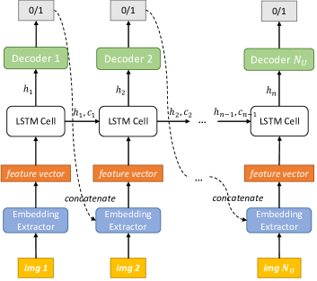
Figure 3: Agent architecture. Each LSTM cell processes an image and outputs a hidden vector to be decoded to a 2D decision vector. We adopt parameter-sharing cell among all units while use different controllers for different AL cycles.

3.4 MAGRAL Controller Training Pipeline

As mentioned above, in order to associate the performance of downstream task learner and the sampling agent, we utilized the detection model to perform proxy task, derived the performance variation and used it as the reward to optimize the agent. In this section, we’ll describe the training pipeline of controller and illustrate the calculation method of reward assisted with semi-supervised learning.

Reward Design. The design of agent reward is the key of our MAGRAL. Because sampled instances are expected to maximize the model performance, we directly take the variation of network performance $\Delta\text{MeanAP}$ as the reward.

Then, for each iteration $i$, we employ the combination of existing labeled samples and the selected unlabeled samples at this iteration $(X_{L}\cup X_{S}^{i})$ to train the task model and obtain the evaluation result $\text{MeanAP}_{i}$. Subsequently, we calculate the difference between $\text{MeanAP}_{i}$ and $\text{MeanAP}_{i-1}$, utilizing it as the reward for our algorithm.

Estimation of Performance Variation of Task Model. Next, here is a problem that the newly selected images are unlabeled and cannot be used in fully supervised model training. However, it occurred to us that the semi-supervised model achieved similar results with the fully-supervised one in object detection [30]. Therefore, we utilize a semi-supervised detector as the proxy task instead when we train the agent and get an estimate of real MeanAP.

We also illustrate the training pipeline in Algorithm 1. For each iteration, we first use the agent to sample a candidate selection set, then regard these candidate samples as unlabeled data to train the semi-supervised model and take the performance value of semi-supervised model as an estimation of MeanAP to calculate reward of MAGRAL agent.

Algorithm 1 Pseudo Code of MAGRAL Training

Input: Labeled pool $X_{L}$, Unlabeled pool $X_{U}$, Task model $M$, Controller $C$
Output: Selected samples at each cycle $S_{t}$, MeanAP of deep model at each cycle mAP_t

1:  for $t=1$ to total_cycles do

2:     Initialize controller $C$

3:     for $i=1$ to max_search_iters do

4:        Initialize task model $M$

5:        $S_{t}^{i}=C.$sample$(X_{U})$

6:        mAP${}_{i}=$ semi_train$(M$, label=$X_{L}$, unl=$S_{t}^{i})$

7:        Optimize $C$ with mAP_i

8:     end for

9:     $S_{t}=C.$sample$(X_{U})$

10:     Annotate selected samples $S_{t}$

11:     $X_{L}=X_{L}\cup S_{t}$

12:     $X_{U}=X_{U}\ \backslash\ S_{t}$

13:     mAP_t= semi_train$(M$, label=$X_{L}$, unl=$X_{U})$

14:  end for

3.5 Acceleration Technique

When training MAGRAL, after agent outputs selected samples for each iteration, we are required to train the semi-supervised detector completely once to obtain the change of model performance, that is $\Delta\text{MeanAP}$. However, training a detection model is quite time-consuming and the number of search iterations is large, which results in the total training time of MAGRAL unacceptable. Therefore, in this section, we propose fast lookup table technique to reduce total time.

Fast lookup table is a commonly used technique that trades space for time. In this problem, we prepare a fast lookup table in advance to assist in estimating MeanAP of different candidate indices when training the agent. We first pre-compute a number of evaluation results of models using different randomly-generated data lists whose size is equal to the labeled pool $X_{L}$ at corresponding AL cycle. Then, we build up the table with records consisting of two pieces of content, one is the list of generated image IDs and the other is the performance trained with these data.

After that, when we start to train the MAGRAL agent, we do not directly use the selected candidate samples to train the semi-supervised detector. Instead, we compare the similarity between the sampled indices and the pre-generated ones in the look-up table and choose the $M$ most similar records on the table. The similarity of two image ID lists is defined as the L2 distance between the vectors derived from performing one-hot coding on the two image indices respectively. Finally, we estimate the MeanAP by conducting weighted summation of the $M$ pre-trained performance values.

Besides, it’s worth illustrating how to generate the fast lookup table more detailedly. We use the same notations as Algorithm 1. Then, if we assume there are $T$ AL cycles in total and it’s required to generate $N_{seed}$ records for each cycle, there will be $T\times N_{seed}$ records totally in the table. Next, for each experiment at cycle $t$, we first generate a batch of images ($N_{L}^{t}$ images) whose size is equal to the labeled samples after cycle $t$. Then, we split the data into two groups, one consists of $N_{L}^{t-1}$ images playing the role of labeled data, and the other contains ($N_{L}^{t}-N_{L}^{t-1}=K$) (the sample size for each cycle) images playing the role of unlabeled data, simulating that $K$ images are selected by the MAGRAL agent for each iteration. After that, the semi-supervised model is trained using these two datasets and performs evaluation to obtain a MeanAP record.

Empirical experiments demonstrate the fast lookup table technique greatly reduces the training time of MAGRAL.

3.6 Optimization Method

There are two sets of parameters that need to be optimized in MAGRAL: the selection agent’s (denoted as $\theta$); and the task learner’s (denoted as $\omega$). At first, we randomly select images from the dataset to initialize the labeled set and utilize the rest as unlabeled. Then we carry on cycle 1’s agent training as in Algorithm 1.

For each iteration, a candidate set of selected images are firstly sampled by the controller $\theta$. With $\theta$ fixed, we train the semi-supervised detection model $\omega$ completely and perform inference to obtain MeanAP. Next, we maintain the detector parameters $\omega$ fixed while updating the agent parameters $\theta$ using reinforcement learning, with $\Delta\text{MeanAP}$ serving as reward $R(\theta)$. Additionally, we implement a moving average baseline inspired by [32] to facilitate training.

$$\begin{split}loss&=-(reward-baseline)\\ baseline&=\lambda*baseline+(1-\lambda)*reward\end{split}$$ (2)

We repeat this process for $max\_search\_iters$ times and employ the trained agent to pick out the most informative samples at this cycle. After that, we use the selected samples to update the labeled and unlabeled pools, reinitialize a new sampling agent and proceed to the next AL cycle.

4 Experiments

In this part, we report the experimental results and analyze the efficiency of MeanAP-guided metric.

4.1 Experimental Settings

Datasets. We use PASCAL VOC [8] and MS COCO [22] to evaluate our MAGRAL. For PASCAL VOC, we utilize VOC2007 and VOC2012 trainval containing $16551$ images in total from $20$ classes as training set, and employ VOC2007 test containing $4952$ images to evaluate MeanAP. MS-COCO is a larger dataset containing images from 80 object categories with more challenging samples. And we use train2017 with $117k$ images for training and val2017 with $5k$ images for evaluation.

Active Learning Settings. For PASCAL VOC, we follow the common settings in LL4AL [31] and MI-AOD [32] to conduct a fair comparison, where the initialized labeled pool contains 1k images and the budget of selected samples at each cycle is also 1k. The total AL cycle is 10. And we use ISD-SSD [15] with VGG-16 [27] as the semi-supervised detector. The model is trained for 300 epochs with mini-batch size 32 and the $\text{learning\_rate}=0.001$ for the first 240 epochs while $0.0001$ for the last 60 epochs. For MS COCO, according to MI-AOD, we set the proportion of initial labeled images as 2.0% and sample 2.0% images from the unlabeled pool at each cycle until achieving 10.0% of training set. Moreover, we deploy SED-SSOD [12] with RetinaNet [21] as semi-supervised model and make mini-batch size 8 and learning rate 0.02.

Besides, we set the dimension of feature vector of our controller as 257 (256 for image embeddings and 1 for decision of previous cell) and utilize a pre-trained network to extract the image embeddings. The hidden and state size of LSTM Cell are thus 257. We train our MAGRAL agent with Adam optimizer [16] at the learning rate of $3.5\times 10^{-2}$ and set the search iteration as $2200$ for a PASCAL VOC AL cycle while $800$ for a COCO AL cycle. And the baseline decay of reward is weighted by $0.5$.

Fast Lookup Table Settings. As mentioned above, we leverage the fast lookup table to speed up the detector training. For PASCAL VOC, we also employ ISD-SSD [15] to build up the lookup table, simulate the results for each of the 10 sampling points respectively and randomly select 1k images at each cycle to perform as the candidate list. Due to the huge search space brought by the combination explosion of pool-based AL methods, for each sampling point, we complete more than 200 pre-trained experiments (i.e., $N_{seed}=200$) to get an estimate as accurate as possible.

For MS COCO, there are 5 AL cycles and $2\%(\sim 2340)$ images are selected in each cycle to perform semi-supervised learning. And we create a fast look up table containing 30 records (i.e., $30\times 5$ pre-trained experiments on COCO) with SED-SSOD [12].

Besides, we adopt multiple sampling methods to generate image lists, so that our pre-compute table could take every image into consideration for the subsequent image search. We take $M=10$ for the similarity calculation and leverage the fitting method to estimate accurate value of MeanAP.

4.2 Model Performance

We compare MAGRAL with random sampling, entropy sampling, Core-set [26], CDAL [1], LL4AL [31] and MI-AOD [32]. We implement entropy sampling by utilizing the average instance entropy as image uncertainty.

PASCAL VOC. We report the performance of MAGRAL on four GTX 1080Ti GPU and consider the results of other methods provided in MI-AOD [32]. To solely focus on active learning, we compare the performance of different methods based on the same detector, SSD [24]. And we use exactly the same initial labeled set as MI-AOD for a fair comparison. The results are shown in Table 1 and Figure 4.

Table 1: Performance results of different active learning methods on PASCAL VOC with SSD.

Method	1k	2k	3k	4k	5k	6k	7k	8k	9k	10k
Random	51.02	60.99	64.60	66.61	67.55	68.90	69.48	70.01	70.70	71.51
Entropy	51.02	61.01	63.58	66.80	68.63	69.80	70.39	71.40	71.82	72.51
Core-set (ICLR 18)	51.02	62.00	66.18	67.81	69.02	69.52	70.80	71.01	71.39	72.02
LL4AL (CVPR 19)	51.02	60.80	65.01	66.97	69.09	70.51	71.50	72.00	73.02	73.31
CDAL (ECCV 20)	51.02	62.04	65.28	67.70	70.01	71.32	72.20	73.18	74.11	75.40
MI-AOD (CVPR 21)	53.62	62.86	66.83	69.33	70.80	72.21	72.84	73.74	74.18	74.91
MAGRAL (Ours)	56.41	63.26	68.09	70.30	72.05	73.16	73.96	74.94	75.41	75.85

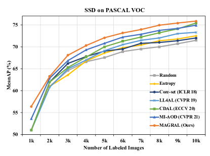
Figure 4: Performance comparison of MAGRAL and other active object detection approaches on PASCAL VOC with SSD. MI-AOD is the current state-of-the-art method.

MAGRAL outperforms state-of-the-art methods with a large margin. And the improvements illustrate the effectiveness of MAGRAL by utilizing MeanAP directly to guide the informative sample selection.

What’s more, it deserves to point out that MAGRAL and MI-AOD surpass other approaches greatly in almost all cycles because they leverage the information of unlabeled data by semi-supervised learning. MI-AOD implicitly embeds semi-supervised training into its query strategy, while our MAGRAL explicitly splits the two parts and connects them by RL. This way makes MAGRAL can use different semi-supervised models and have better flexibility to migrate to other models or tasks. We will discuss it more deeply later.

MS COCO. We complete the experiments on four Tesla V100 32G GPUs. And all results are based on RetinaNet [21]. We also use the same initial labeled set as MI-AOD. The results are shown in Table 2. It can be seen that MAGRAL also performs well and beats other methods on MS COCO.

Table 2: Results of different AL methods on MS COCO.

Method	2.0%	4.0%	6.0%	8.0%	10.0%
Random	6.70	13.20	15.70	17.90	19.00
Entropy	6.70	12.90	14.90	16.40	17.40
Core-set (ICLR 18)	6.70	13.30	16.00	17.50	18.80
MI-AOD (CVPR 21)	7.40	13.80	16.90	19.10	20.80
MAGRAL (Ours)	7.40	14.50	17.90	20.00	22.20

Table 3: Difference between MeanAP and uncertainty.

# of Labeled	2000		5000
List id	MeanAP	Entropy	MeanAP	Entropy
1	59.28	1108.22	68.25	2761.89
2	58.85	1100.26	69.35	2802.20
3	60.45	1096.61	68.71	2755.52
4	60.42	1124.13	68.15	2767.83
5	59.95	1099.97	67.77	2754.33

4.3 Visualization Results of Selected Samples by Multiple AL Methods

We visualize some images selected by different query strategies at the first AL cycle in Figure 5. The five images in the first row are selected by the mean entropy sampling (the three on the top left) and sum entropy sampling (the two on the top right), while the second row and third row display the images sampled by MI-AOD [32] and our MAGRAL. It can be seen that the images sampled by mean entropy appear to be exposed or blurred, which makes object detection very difficult. But the aim of AL is to select samples that benefit the model learning best, not select the hardest that the model cannot learn. The images derived using the sum of instance entropy is shown to contain multiple objects, but most of which belong to the same category, bringing redundant information. MI-AOD and our method both select images with only one object locating in the center of the image. Despite these images are easy for detection, they are essential for a well-performed detector to learn generalized information. And our method select images with more categories than MI-AOD, which helps the detector to be more robust in test set and improves the performance MeanAP.

4.4 Ablation Study and Analysis

Difference between MeanAP-guided Metric and Uncertainty. We calculate the uncertainty (mean entropy) and MeanAP of different image lists with 2000 and 5000 labeled images on PASCAL VOC respectively in Tab.3. It’s obvious that a high MeanAP does not mean a high entropy and vice versa. So, the hand-crafted uncertainty is not always equal to the task model performance exactly.

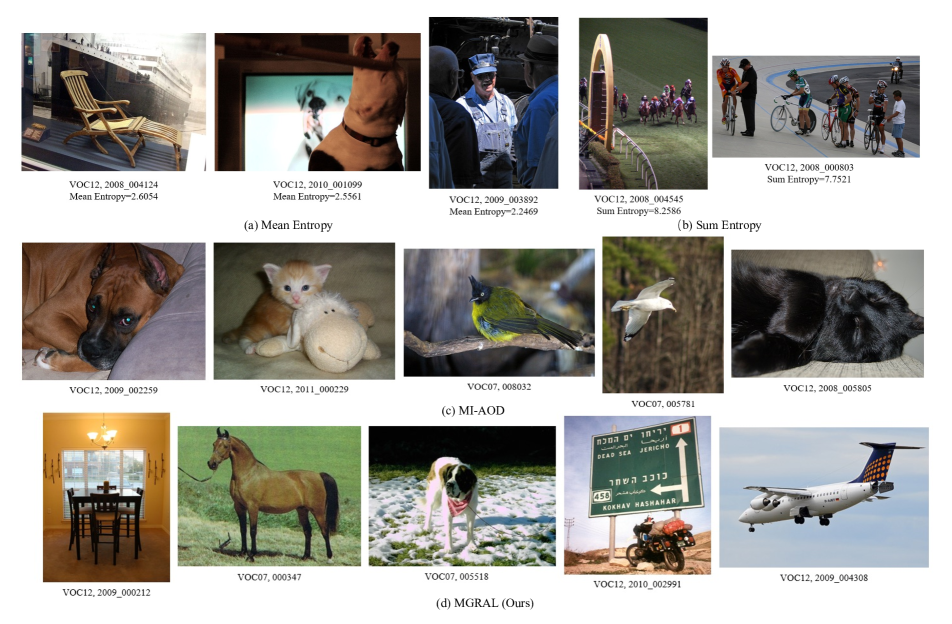
Figure 5: Visualization results of selected samples by MAGRAL and other state-of-the-art methods at the first AL cycle on PASCAL VOC. The first row contains images selected by using the mean entropy or sum entropy of instances as image uncertainty. The second row is the result of MI-AOD. And the last row consists of images sampled by MAGRAL.

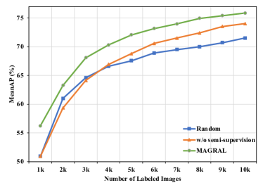
Figure 6: Ablation study on semi-supervised learning.

Semi-supervised Model and Its Effect. Inspired by MI-AOD[32], MAGRAL also combines semi-supervised learning (SSL) to boost the performance. We conduct ablation study on the model without SSL to validate its effect.

As shown in Figure 6, the performance curve of the model without SSL is worse than random sampling using 2k and 3k labeled samples while better when using more than 4k labeled images. The results also manifest a trend that the improvements made by the model without SSL increase as more labeled samples are utilized.

From our perspective, there are two main reasons. Firstly, because MAGRAL employs the semi-supervised model to perform proxy task during training, the selected samples best suit the model with SSL. However, to conduct a fair comparison, we verify the AL performance with the model that does not use SSL. So, the AL performance naturally drops. Secondly, when there are few labeled samples, the information that task learner grasp is not enough to provide a good reward to guide the data selection. Therefore, in the first few cycles, the semi-supervised mechanism plays a more important role and effectively improves the MeanAP of detector. But, with the increase of labeled samples, the performance of model without SSL enhances and narrows the gap towards MAGRAL. It once again reflects MeanAP-guided method has the characteristic of model specificity and verifies our assumptions in the motivation.

Table 4: Estimation accuracy of fast lookup table.

	2000 imgs		3000 imgs		5000 imgs		7000 imgs
id	Acc	Pred	Acc	Pred	Acc	Pred	Acc	Pred
1	55.88	54.03	61.42	61.55	69.26	71.21	73.72	74.04
2	55.64	54.82	63.95	62.22	70.31	70.81	72.94	73.83
3	57.83	55.33	63.86	63.91	70.59	70.97	73.52	74.13
4	56.41	53.54	63.80	63.41	70.43	70.89	73.86	74.20
5	52.53	52.72	63.28	63.23	70.77	71.33	73.59	73.69
6	55.61	54.52	64.29	63.43	69.94	71.22	73.90	74.05
7	55.41	54.65	63.98	62.40	69.06	71.22	73.67	73.89
8	55.11	55.38	63.83	64.08	69.73	70.76	73.96	73.82
Avg	-1.17		-0.52		1.04		0.31
Max	-2.87		-1.73		2.16		0.89

Performance of Fast Lookup Table Technique.

i) Estimation Accuracy on MeanAP. As shown in Tab.4, we randomly select 8 groups of pre-generated sequences and compare the estimated MeanAP with true values. We report the results with 2k, 3k, 5k and 7k sampled images. And the estimated values are biased unilaterally at the same column ensuring the size relationship of MeanAP of different records. Besides, we conducted experiments utilizing look up tables of different sizes, details of which are shown in Appendix B. Through the results, we find that MAGRAL is irrelevant to some specific records of the table and performs well as long as the lookup table contains a minimum threshold of data records.

ii) Training Efficiency. We show the time cost of our method w/ and w/o lookup table in Tab. 5. It took us about 3 minutes to train the agent for ten iterations when having lookup table compared to 80 hours otherwise. Moreover, MAGRAL only spent 10.6 hours training a complete sampling agent. We additionally compare the efficiency of MAGRAL with other methods in Appendix A.

Table 5: Time cost w/ or w/o lookup table on PASCAL VOC.

Method	10 iterations	Total for an AL cycle
w/ lookup table	3 min	640 min
w/o acceleration	4800 min	unknown

5 Conclusion

In this paper, we propose a MeanAP-Guided Reinforced Active Learning method (MAGRAL) for object detection task. MAGRAL substitutes MeanAP-guided strategy for previous uncertainty-based or distribution-based policy through employing a RL-based sampling agent. MAGRAL utilizes LSTM to implement the agent and uses $\Delta\text{MeanAP}$ as the reward. We also introduce an acceleration technique, fast lookup table to speed up the training. Empirical experiments demonstrate the state-of-the-art performance of MAGRAL. Moreover, our method can easily migrate to other models or tasks by replacing MeanAP with specific metrics. MAGRAL lays a solid baseline for reinforced active object detection.

Table 6: MAGRAL performance on PASCAL VOC with various sizes of the fast lookup table.

Look-up Table	1000	2000	3000	4000	5000	6000	7000	8000	9000	10000
50 records	56.41	62.95	67.22	70.33	72.12	73.04	74.04	74.83	75.57	75.82
100 records	56.41	62.91	67.56	69.82	72.38	72.82	73.90	74.46	75.02	75.57
200 records (Ours)	56.41	63.26	68.09	70.30	72.05	73.16	73.96	74.94	75.41	75.85

Table 7: Experiments about one agent for all cycles on PASCAL VOC.

Method	1000	2000	3000	4000	5000	6000	7000	8000	9000	10000
Multi-agents (Ours)	56.41	63.26	68.09	70.30	72.05	73.16	73.96	74.94	75.41	75.85
One-agent	56.41	63.66	68.11	70.84	72.56	73.58	74.61	75.11	75.38	75.65

Appendix A Training Efficiency

A.1 Efficiency of Fast Lookup Table.

As shown in Table 5, we tested the efficiency of different methods on four GTX 1080Ti GPU. It took us about 4800 minutes (80 hours) to train a MAGRAL agent for ten iterations as it required us to train the semi-supervised detector from scratch ten times, which was intolerable. As a comparison, the algorithm using fast lookup table technique only spent 3 minutes on ten iteration training and 640 minutes (10.6 hours) in training a complete MAGRAL agent.

A.2 Comparison of Training Efficiency.

We report the training and inference time of entropy sampling, MI-AOD [32] and our MAGRAL on PASCAL VOC in Tab.8. And we report the time at the first AL cycle because it takes us the longest time to train the neural network. Experiments are conducted on a GTX 1080Ti GPU. And in the table, the time enclosed by ”()” is the time required to create the lookup table. On PASCAL VOC, it took us about $9$ hours to train different ISD-SSD [15] models with different groups of data in parallel (training each model with two GTX 1080Ti GPUs) to generate the fast lookup table. Although MAGRAL needs more time for training, it has a shorter inference time which concerns more in practice.

Table 8: Training efficiency of different methods on PASCAL VOC at the first Active Learning cycle.

Method	Training Time	Inference Time
Entropy	0	5 min
MI-AOD (CVPR 21)	7 h 13 min	43 min
MAGRAL (Ours)	(9 hours) + 7 h 8 min	0.5 min

Appendix B MAGRAL Performance with Various Sizes of the Fast Lookup Table.

For Pascal VOC, we reported the results in the main body with a fast look up table containing $200$ records ($200\times 10$ pre-trained experiments). And we conducted experiments utilizing $50$-record and $100$-record look up tables respectively to train our MAGRAL. The results are shown in Table 6. From the table, we can see that the performances of MAGRAL do not have perceptible change with the variation of the number of pre-trained experiments (records). It proves that our method is irrelevant to some specific records of the table and MAGRAL performs well as long as the look up table has a certain size.

Appendix C Experiments on One Agent for All Cycles

In our MAGRAL, we originally trained one agent for each cycle because the distribution of labeled data which the task model learned would change after new samples were selected and added to the labeled pool. However, we have also explored how about utilizing the agent learned at the first cycle to select the most informative samples to be annotated for all the consecutive 9 cycles. The results are shown in Tab.7. We found that it performed better than the original method in the first 7 cycles, but the performance improvements of it gradually decreased as the number of cycles increased. Therefore, we can conclude that in the first few cycles, the data distribution does not change greatly, so with the agent learned at the first cycle which stores maximum information about data distribution, it performs well. However, after a few cycles, the agent cannot further represent the distribution and thus hurts the performance. And on this basis, we think although the one-agent method is more suitable for active learning settings and more efficient for training, the generalization ability of agent to adapt to data distribution cannot be guaranteed.

References

- [1] Sharat Agarwal, Himanshu Arora, Saket Anand, and Chetan Arora. Contextual diversity for active learning. In Computer Vision - ECCV 2020 - 16th European Conference, Glasgow, UK, August 23-28, 2020, Proceedings, Part XVI, volume 12361 of Lecture Notes in Computer Science, pages 137–153. Springer, 2020.
- [2] Hamed H. Aghdam, Abel Gonzalez-Garcia, Antonio M. López, and Joost van de Weijer. Active learning for deep detection neural networks. In 2019 IEEE/CVF International Conference on Computer Vision, ICCV 2019, Seoul, Korea (South), October 27 - November 2, 2019, pages 3671–3679. IEEE, 2019.
- [3] Philip Bachman, Alessandro Sordoni, and Adam Trischler. Learning algorithms for active learning. In Doina Precup and Yee Whye Teh, editors, Proceedings of the 34th International Conference on Machine Learning, ICML 2017, Sydney, NSW, Australia, 6-11 August 2017, volume 70 of Proceedings of Machine Learning Research, pages 301–310. PMLR, 2017.
- [4] Arantxa Casanova, Pedro O. Pinheiro, Negar Rostamzadeh, and Christopher J. Pal. Reinforced active learning for image segmentation. In 8th International Conference on Learning Representations, ICLR 2020, Addis Ababa, Ethiopia, April 26-30, 2020. OpenReview.net, 2020.
- [5] Gabriella Contardo, Ludovic Denoyer, and Thierry Artières. A meta-learning approach to one-step active-learning. In Proceedings of the International Workshop on Automatic Selection, Configuration and Composition of Machine Learning Algorithms co-located with the European Conference on Machine Learning & Principles and Practice of Knowledge Discovery in Databases, AutoML@PKDD/ECML 2017, Skopje, Macedonia, September 22, 2017, pages 28–40. CEUR-WS.org, 2017.
- [6] Ido Dagan and Sean P Engelson. Committee-based sampling for training probabilistic classifiers. In Machine Learning Proceedings 1995, pages 150–157. Elsevier, 1995.
- [7] David L Donoho et al. High-dimensional data analysis: The curses and blessings of dimensionality. AMS math challenges lecture, 1(2000):32, 2000.
- [8] Mark Everingham, Luc Van Gool, Christopher KI Williams, John Winn, and Andrew Zisserman. The pascal visual object classes (voc) challenge. International journal of computer vision, 88(2):303–338, 2010.
- [9] Yoav Freund, H Sebastian Seung, Eli Shamir, and Naftali Tishby. Information, prediction, and query by committee. Advances in neural information processing systems, 5:483–490, 1992.
- [10] Yarin Gal, Riashat Islam, and Zoubin Ghahramani. Deep bayesian active learning with image data. In Doina Precup and Yee Whye Teh, editors, Proceedings of the 34th International Conference on Machine Learning, ICML 2017, Sydney, NSW, Australia, 6-11 August 2017, volume 70 of Proceedings of Machine Learning Research, pages 1183–1192. PMLR, 2017.
- [11] Daniel Golovin, Andreas Krause, and Debajyoti Ray. Near-optimal bayesian active learning with noisy observations. pages 766–774, 2010.
- [12] Qiushan Guo, Yao Mu, Jianyu Chen, Tianqi Wang, Yizhou Yu, and Ping Luo. Scale-equivalent distillation for semi-supervised object detection. In Proceedings of the IEEE/CVF Conference on Computer Vision and Pattern Recognition, pages 14522–14531, 2022.
- [13] Sepp Hochreiter and Jürgen Schmidhuber. Long short-term memory. Neural computation, 9(8):1735–1780, 1997.
- [14] Suyog Dutt Jain and Kristen Grauman. Active image segmentation propagation. In Proceedings of the IEEE Conference on Computer Vision and Pattern Recognition, pages 2864–2873. IEEE Computer Society, 2016.
- [15] Jisoo Jeong, Vikas Verma, Minsung Hyun, Juho Kannala, and Nojun Kwak. Interpolation-based semi-supervised learning for object detection. In Proceedings of the IEEE/CVF Conference on Computer Vision and Pattern Recognition, pages 11602–11611. Computer Vision Foundation / IEEE, 2021.
- [16] Diederik P. Kingma and Jimmy Ba. Adam: A method for stochastic optimization. 2015.
- [17] Ksenia Konyushkova, Raphael Sznitman, and Pascal Fua. Discovering general-purpose active learning strategies, 2018.
- [18] Satoshi Kosugi, Toshihiko Yamasaki, and Kiyoharu Aizawa. Object-aware instance labeling for weakly supervised object detection. In Proceedings of the IEEE/CVF International Conference on Computer Vision, pages 6063–6071. IEEE, 2019.
- [19] Weicheng Kuo, Christian Häne, Esther L. Yuh, Pratik Mukherjee, and Jitendra Malik. Cost-sensitive active learning for intracranial hemorrhage detection. In Medical Image Computing and Computer Assisted Intervention - MICCAI 2018 - 21st International Conference, Granada, Spain, September 16-20, 2018, Proceedings, Part III, volume 11072 of Lecture Notes in Computer Science, pages 715–723. Springer, 2018.
- [20] Xin Li and Yuhong Guo. Adaptive active learning for image classification. In 2013 IEEE Conference on Computer Vision and Pattern Recognition, Portland, OR, USA, June 23-28, 2013, pages 859–866. IEEE Computer Society, 2013.
- [21] Tsung-Yi Lin, Priya Goyal, Ross Girshick, Kaiming He, and Piotr Dollár. Focal loss for dense object detection. In Proceedings of the IEEE international conference on computer vision, pages 2980–2988, 2017.
- [22] Tsung-Yi Lin, Michael Maire, Serge Belongie, James Hays, Pietro Perona, Deva Ramanan, Piotr Dollár, and C Lawrence Zitnick. Microsoft coco: Common objects in context. In European conference on computer vision, pages 740–755. Springer, 2014.
- [23] Ming Liu, Wray Buntine, and Gholamreza Haffari. Learning how to actively learn: A deep imitation learning approach. In Proceedings of the 56th Annual Meeting of the Association for Computational Linguistics (Volume 1: Long Papers), pages 1874–1883, 2018.
- [24] Wei Liu, Dragomir Anguelov, Dumitru Erhan, Christian Szegedy, Scott E. Reed, Cheng-Yang Fu, and Alexander C. Berg. SSD: single shot multibox detector. In Computer Vision - ECCV 2016 - 14th European Conference, Amsterdam, The Netherlands, October 11-14, 2016, Proceedings, Part I, volume 9905 of Lecture Notes in Computer Science, pages 21–37. Springer, 2016.
- [25] Thomas Osugi, Deng Kim, and Stephen Scott. Balancing exploration and exploitation: A new algorithm for active machine learning. In Fifth IEEE International Conference on Data Mining (ICDM’05), pages 8–pp. IEEE, 2005.
- [26] Ozan Sener and Silvio Savarese. Active learning for convolutional neural networks: A core-set approach. In 6th International Conference on Learning Representations, ICLR 2018, Vancouver, BC, Canada, April 30 - May 3, 2018, Conference Track Proceedings. OpenReview.net, 2018.
- [27] Karen Simonyan and Andrew Zisserman. Very deep convolutional networks for large-scale image recognition. 2015.
- [28] Samarth Sinha, Sayna Ebrahimi, and Trevor Darrell. Variational adversarial active learning. In Proceedings of the IEEE/CVF International Conference on Computer Vision, pages 5972–5981, 2019.
- [29] Lin Yang, Yizhe Zhang, Jianxu Chen, Siyuan Zhang, and Danny Z Chen. Suggestive annotation: A deep active learning framework for biomedical image segmentation. In International conference on medical image computing and computer-assisted intervention, pages 399–407. Springer, 2017.
- [30] Qize Yang, Xihan Wei, Biao Wang, Xian-Sheng Hua, and Lei Zhang. Interactive self-training with mean teachers for semi-supervised object detection. In Proceedings of the IEEE/CVF Conference on Computer Vision and Pattern Recognition, pages 5941–5950, 2021.
- [31] Donggeun Yoo and In So Kweon. Learning loss for active learning. In Proceedings of the IEEE/CVF conference on computer vision and pattern recognition, pages 93–102, 2019.
- [32] Tianning Yuan, Fang Wan, Mengying Fu, Jianzhuang Liu, Songcen Xu, Xiangyang Ji, and Qixiang Ye. Multiple instance active learning for object detection. In Proceedings of the IEEE/CVF Conference on Computer Vision and Pattern Recognition, pages 5330–5339, 2021.
- [33] Xiaosong Zhang, Fang Wan, Chang Liu, Rongrong Ji, and Qixiang Ye. Freeanchor: Learning to match anchors for visual object detection. pages 147–155, 2019.
- [34] Xiaosong Zhang, Fang Wan, Chang Liu, Xiangyang Ji, and Qixiang Ye. Learning to match anchors for visual object detection. IEEE Transactions on Pattern Analysis and Machine Intelligence, 2021.
- [35] Barret Zoph and Quoc V. Le. Neural architecture search with reinforcement learning. In 5th International Conference on Learning Representations, ICLR 2017, Toulon, France, April 24-26, 2017, Conference Track Proceedings. OpenReview.net, 2017.