Data Driven Modeling for Self-Similar Dynamics

Abstract

Multiscale modeling of complex systems is crucial for understanding their intricacies. Data-driven multiscale modeling has emerged as a promising approach to tackle challenges associated with complex systems. On the other hand, self-similarity is prevalent in complex systems, hinting that large-scale complex systems can be modeled at a reduced cost. In this paper, we introduce a multiscale neural network framework that incorporates self-similarity as prior knowledge, facilitating the modeling of self-similar dynamical systems. For deterministic dynamics, our framework can discern whether the dynamics are self-similar. For uncertain dynamics, it not only can judge whether it is self-similar or not, but also can compare and determine which parameter set is closer to self-similarity. The framework allows us to extract scale-invariant kernels from the dynamics for modeling at any scale. Moreover, our method can identify the power-law exponents in self-similar systems, providing valuable insights for addressing critical phase transitions in non-equilibrium systems.

1 Introduction

Complex systems modeling is essential for understanding, predicting, and even controlling a complex system. Due to the non-linear, self-organizing, emergence, and other complex behaviors in them, modeling complex systems has always been challenging. In recent decades, data-driven approaches, leading by machine learning, have shown significant advantages in so many fields, which inspired us to do better in modeling complex systems. On the other hand, self-similarity is a common feature of complex systems. From natural systems, like the fractal structure of vegetation clusters in the Amazon rainforest and the Tibetan plateau[1], the critical phenomena in atmospheric precipitation[2], to societal systems like network traffic[3], the avalanche of public opinion in social medias[4], and neural system like critical phenomenon in brain[5, 6, 7, 8] and so on, there are so many evidences of scale-invariant properties in complex systems. Thus, we’re motivated to integrate self-similarity as prior knowledge, aiming for data-driven multi-scale modeling of complex systems.

Two aspects of modeling complex systems are network structure and dynamics. The concept of self-similarity in networks was proposed in [9], leading to explorations of multiscale network modeling[10, 11, 12, 13, 14, 15, 16]. This offers insights into modeling large-scale systems more cost-effectively. Discussions integrating dynamics with self-similarity in complex system modeling have been relatively scarce. By combining multiscale dynamics with self-similarity, maybe we can model complex dynamic systems with fewer parameters, and capture the scale-invariant key features.

A related field is dynamic reduction[17, 18], which seeks lower-dimensional representations of systems and their dynamics. It aims to reproduce high-dimensional dynamics at microscopic level with simpler models. Although not explicitly stated, it also implies the dynamics has self-similarity of the predicted results at different scales. But they neither considered whether the low-dimensional representation has physical meaning nor discussed self-similarity.

Another related topic is renormalization group (RG) theory[19, 20, 21]. RG theory deals with how system parameters vary with scale, which is essential in condensed matter physics for addressing phase transitions and critical phenomena, and it does touch upon self-similarity. In this context, self-similarity means the system remains unchanged at a fixed point in parameter space. RG theory has been successful for solving the problems in equilibrium systems. Furthermore, Theoretical physicists also invented the theory of dynamic RG to describe how a dynamic system parameters change with scale[22, 23, 24], and try to use it to solve the critical problems in non-equilibrium systems. However, due to the complexity of dynamic systems, the analysis of dynamic RG involves intricate mathematical techniques. On one hand, it heavily depends on the researcher’s expertise. On the other, it’s currently limited to analyzing very basic systems, like kinetic Ising model[25, 26], sandpile model[27, 28, 29] and Viseck model[30, 31, 32],etc. And There are also subjective renormalization strategies, where different strategies might lead to varying results. It also adds difficulty to the theory’s direct application in complex dynamic systems.

Hence, analytical solutions and simple models are insufficient for complex systems, but data-driven methods might be the way forward. Physics-informed machine learning has seen recent success in numerous domains[33, 34, 35]. Designing neural network architectures based on inductive biases is considered the most principled way of making a learning algorithm informed by physics[33]. Among them, there are many multi-scale neural network architectures are introduced for improved predictions, but these frameworks focus on specific tasks and don’t discuss the system’s self-similarity features. At the same time, integrating renormalization theory and machine learning has seen progress[36, 37, 38, 39, 40, 41, 42, 43, 44], but most research focuses on static systems without considering dynamics.

Based on the above background, we introduce a multi-scale neural network framework that integrates self-similarity priors for modeling complex dynamic systems.

Our contributions include:

• By introducing self-similarity as the prior information of model design, our framework can identify if the dynamic systems are self-similar, whether deterministic or stochastic dynamics.

• Our framework can automatically learn the dynamic renormalization strategies.

• Our framework can automatically capture scale-invariant kernel in dynamics, which means we use fewer parameters to model the dynamic system.

The structure of the article is as follows: In section 2, we give the formal definition of self-similar dynamics, and give our model framework design idea. In the experimental part, we use two examples to illustrate the feasibility of the model in section 3. At last, we discuss the potential of our framework and its implications for understanding complex dynamical systems.

2 Method

2.1 Definition

Self-similar dynamics, intuitively, means the system’s dynamics are consistent or similar across multiple scales. This doesn’t just refer to the form of the dynamics but also their parameters. Based on this intuition, let’s provide a formal definition. We define the microstates of a system as $\boldsymbol{X}\in\mathbb{R}^{n^{d}}$, where $n^{d}$ represents the size of the space $\boldsymbol{X}$ occupies, indicating the possible $n^{d}$ components of $\boldsymbol{x_{i}}$, and $d$ is the spatial dimension of the system. Its micro dynamics is given by $\Delta\boldsymbol{X}=f(\boldsymbol{X},\boldsymbol{W})$, where $\boldsymbol{W}$ is the parameters of the dynamics. In our discussion, self-similarity dynamics means that after a system evolves over time following states $\boldsymbol{X}_{0:t_{m}}=\{\boldsymbol{X}_{0},\boldsymbol{X}_{1},\dots,\boldsymbol{X}_{t_{m}}\}$, and is transformed by mapping $P$ to produce $\boldsymbol{Y}\in\mathbb{R}^{N^{d}\times F}$ such that $\boldsymbol{Y}=P({\boldsymbol{X}_{0:t_{m}}})$, both the form and parameter of the micro dynamics remain unchanged or similar to the one in the macro dynamics. This implies an assumption of local behavior in dynamic space. This means that for every microstate component $\boldsymbol{x^{i}}$, the dynamics satisfies

$${\Delta\boldsymbol{x^{i}}}=f^{i}(\boldsymbol{x^{i}},\{\boldsymbol{x^{j}},\forall\boldsymbol{x^{j}}\in Nei(\boldsymbol{x^{i}})\},\boldsymbol{w^{i}}_{local})$$ (1)

Here,$f^{i}$ represents the dynamics of component $\boldsymbol{x^{i}}$. The set $\{\boldsymbol{x^{j}},\forall\boldsymbol{x^{j}}\in Nei(\boldsymbol{x^{i}})\}$ denotes the neighboring states of $i$. $\boldsymbol{w^{i}}_{local}$ is the dynamic parameter for each component $i$. For simplicity, our following discussion focuses on homogeneous dynamics, where all components share the same dynamic parameter $\boldsymbol{w}_{local}$. The mapping $P$ is also a local operation. Let $\boldsymbol{\tilde{X}}^{i}_{t}\in\mathbb{R}^{S^{d}\times T}=\{\boldsymbol{x}^{i-S^{d}}_{t-T},\boldsymbol{x}^{i-S^{d}+1}_{t-T},\dots,\boldsymbol{x}^{i}_{t-T+1},\dots,\boldsymbol{x}^{i}_{t}\}$ be a basic unit within $\boldsymbol{X}_{0:t_{m}}$. It captures the local system state over spatial scale $S$ and temporal scale $T$. So $\boldsymbol{X}_{0:t_{m}}$ can be represented as a collection of these unites, that is $\boldsymbol{X}_{0:t_{m}}=\{\boldsymbol{\tilde{X}}^{0}_{0},\boldsymbol{\tilde{X}}^{1}_{0},\dots,\boldsymbol{\tilde{X}}^{n^{d}/S^{d}}_{0},\boldsymbol{\tilde{X}^{0}_{1}},\dots,\boldsymbol{\tilde{X}}^{n^{d}/S^{d}}_{t_{m}\//T}\}$. For each $\boldsymbol{\tilde{X}}^{i}_{t}$ we have

$$\boldsymbol{y^{i}_{t}}=P_{local}(\boldsymbol{\tilde{X}}^{i}_{t}),P_{local}\in\mathbb{R}^{S^{d}\times T\times 1}$$ (2)

The operator $P_{local}$ maps from $S^{d}\times T$ to 1, as illustrated in Fig.1. Therefore, the global mapping result is equivalent to concatenating each local mapping outcome, which means

$$P(\boldsymbol{X})=P_{local}(\boldsymbol{\tilde{X}}^{0}_{0})\bigoplus P_{local}(\boldsymbol{\tilde{X}}^{1}_{0})\bigoplus\dots\bigoplus P_{local}(\boldsymbol{\tilde{X}}^{n^{d}/S^{d}}_{t_{m}\//T}\})$$ (3)

So in simpler terms, self-similar dynamics means that for every local state $\boldsymbol{\tilde{X}}^{i}_{t}$ of the microscopic system, once mapped to the macrostate $\boldsymbol{x^{i}_{t}}$ by $P_{local}$, the form and parameters $\boldsymbol{w}_{local}$ of each macro-state dynamics $f_{i}$ remain consistent with the micro one. That is, the macro dynamics also follow $\boldsymbol{dy^{i}}\//dt=f(\boldsymbol{y^{i}},\{\boldsymbol{y^{j}},\forall\boldsymbol{y^{j}}\in Nei(\boldsymbol{y^{i}})\},\boldsymbol{w}_{local})$. Such states typically suggest the system is at a fixed point in parameter space, meaning its parameters don’t change with scale. At these times, the system usually exhibits scaling phenomena.

An effective verification method for self-similar dynamics can be carried out using the following steps:

1. Coarse-grain the microstate $\boldsymbol{\tilde{X}}^{i}_{t}$ to obtain $\boldsymbol{y^{i}_{t}}$. Then evolve $\boldsymbol{y^{i}_{t}}$ by one step to get $\boldsymbol{y^{i}_{t+1}}$

$$\boldsymbol{y^{i}_{t+1}}=\boldsymbol{y^{i}_{t}}+f^{i}[P_{local}(\boldsymbol{\tilde{X}}^{i}_{t})]$$ (4)

2. Coarse-grain the microstate $\boldsymbol{\tilde{X}}^{i}_{t+1}$ directly

$$(\boldsymbol{y^{i}_{t+1}})^{\prime}=P_{local}[\boldsymbol{\tilde{X}}^{i}_{t+1}]$$ (5)

3. Compare $\boldsymbol{y^{i}_{t+1}}$ from step 1 and $(\boldsymbol{y^{i}_{t+1}})^{\prime}$ from step 2. If consistent results are obtained, the dynamics can be considered self-similar.

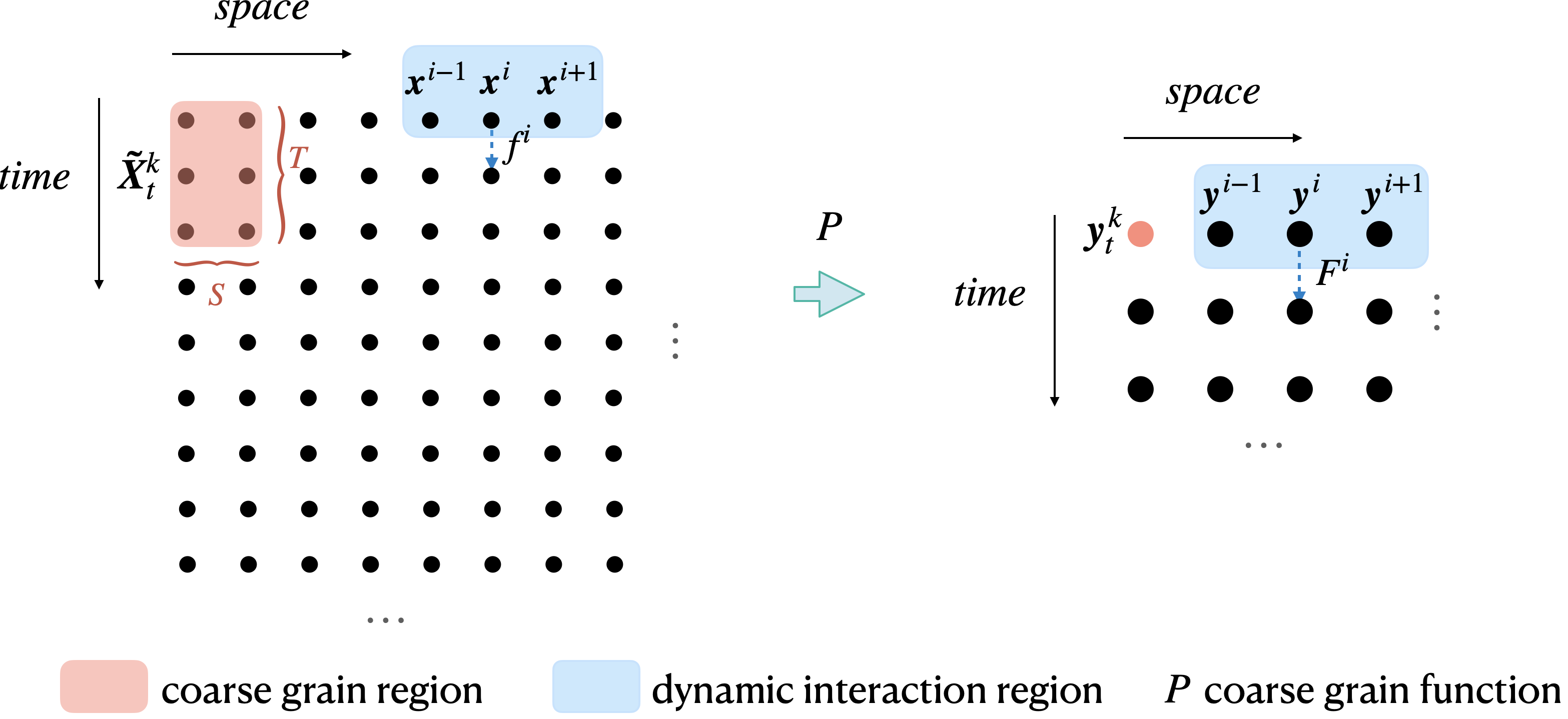
Figure 1: Diagram of localization for dynamics and coarse-graining in lattice systems. The blue area represents the localization of dynamics, here is the nearest neighborhood interaction as an example. Blue dashed arrow means $\boldsymbol{x}^{i}$ or $\boldsymbol{y}^{i}$ evolves one step with dynamic $f^{i}$ or $F^{i}$. The red area represents a basic unit of microstate $\boldsymbol{\tilde{X}}^{k}_{t}$ and it will be coarse-grained as a macrostate $\boldsymbol{y}^{k}_{t}$, displaying as a red point in the figure. Both dynamics and coarse-graining operator could apply to any of other states and areas. The locality of the dynamics and coarse-graining shown here are the key point to self-similar dynamics

2.2 Framework

According to the definition, we utilize a multiscale neural network approach, comprising two main components: a dynamics learner and a coarse-graining learner.

Dynamics Learner: Using micro-level data $\boldsymbol{X}$ to learn the dynamic rules $f(\boldsymbol{\theta_{1}})$, The neural network parameters effectively serve as the dynamic parameters $\boldsymbol{w}_{local}$. The optimization goal is to minimize the difference between the actual value $\boldsymbol{x}_{t+1}$ and the predicted value $\hat{\boldsymbol{x}}_{t+1}$. Considering the differences in data dimensions between the micro and macro scales—with macro variables typically being fewer—it is important to design neural networks that demonstrate spatio-temporal translational invariance. Only in this manner can we potentially apply the dynamics learner, trained on micro-level data, to macro-level data as well.

Coarse-Graining Learner: Learning the mapping from the microstates $\boldsymbol{X}$ to the macrostates $\boldsymbol{Y}$, expressed as $\boldsymbol{Y}=P_{local}(\boldsymbol{X},\boldsymbol{\theta_{2}})$. The objective is to ensure that the learned macrostates $\boldsymbol{Y}$ align with the dynamics $f(\boldsymbol{\theta_{1}})$, that is, the form and the parameters of macro-dynamics should be same as the micro-dynamics, and we could still get an accurate prediction from $\boldsymbol{y}_{t}$ to $\boldsymbol{y}_{t+1}$ according to $f(\boldsymbol{\theta_{1}})$. In other words, the self-similarity in system dynamics is incorporated as a constraint in the model design, guiding the Coarse-graining learner to adhere to this constraint.

The model framework is illustrated in Fig 2. We aim for the predicted microstate $\hat{\boldsymbol{x}}_{t_{m}+1}$ to closely approximate the actual state $\boldsymbol{x}_{t_{m}+1}$, this is the first loss function of our framework in order to optimize the dynamical Learner (Eq.6). For the coarse-grained learner, we incorporate a third decoder neural module $P^{\prime}(\boldsymbol{\theta_{3}})$ to prevent learning trivial coarse-grained rules, such as mapping all states to zero. This is done to ensure that the macro-states $\boldsymbol{y}_{t_{M}+1}$can be effectively decoded back into microstates $\boldsymbol{\tilde{X}}_{t_{M}+1}$. Therefore, the second learning objective of our framework is to make the decoded state $\boldsymbol{\tilde{X}}^{D}_{t_{M}+1}$ as close as possible to the actual state $\boldsymbol{\tilde{X}}_{t_{M}+1}$ (Eq.7). Fig 2 visualizes the whole process with spatial dimension $d=1$. It can be easily extended to higher dimensions.

$$\boldsymbol{\theta_{1}}^{*}=argmin(\|{\boldsymbol{x}}_{t_{m}+1}-f(\boldsymbol{x}_{t_{m}},\boldsymbol{\theta_{1}})\|^{2})$$ (6)

$$\boldsymbol{\theta_{2}}^{*},\boldsymbol{\theta_{3}}^{*} =argmin(\|\boldsymbol{\tilde{X}}_{t_{M}+1}-\boldsymbol{\tilde{X}}^{D}_{t_{M}+1}\|^{2})$$ (7)

$$=argmin(\|\boldsymbol{\tilde{X}}_{t_{M}+1}-P^{\prime}(\boldsymbol{\hat{y}}_{t_{M}+1},\boldsymbol{\theta_{3}})\|^{2})$$

$$=argmin(\|\boldsymbol{\tilde{X}}_{t_{M}+1}-P^{\prime}(f(\boldsymbol{y}_{t_{M}},\boldsymbol{\theta_{1}}^{*}),\boldsymbol{\theta_{3}})\|^{2})$$

$$=argmin(\|\boldsymbol{\tilde{X}}_{t_{M}+1}-P^{\prime}(f(P(\boldsymbol{\tilde{X}}_{t_{M}},\boldsymbol{\theta_{2}}),\boldsymbol{\theta_{1}}^{*}),\boldsymbol{\theta_{3}})\|^{2})$$

Our multiscale framework is inspired by the design in [45], while they used Invertible Neural Networks (INN) in their encoder and decoder to ensure favorable mathematical properties. In our approach, the encoder and decoder are two distinct neural networks. We made this choice to circumvent the efficiency issues encountered during the training of INN. Additionally, our model training is divided into two stages. The first stage achieves optimal dynamics, which is then applied at the macro level in the second stage, rather than training them concurrently. We adopted this approach to ensure the functions of the dynamics and the encoder remain independent and don’t become intertwined.

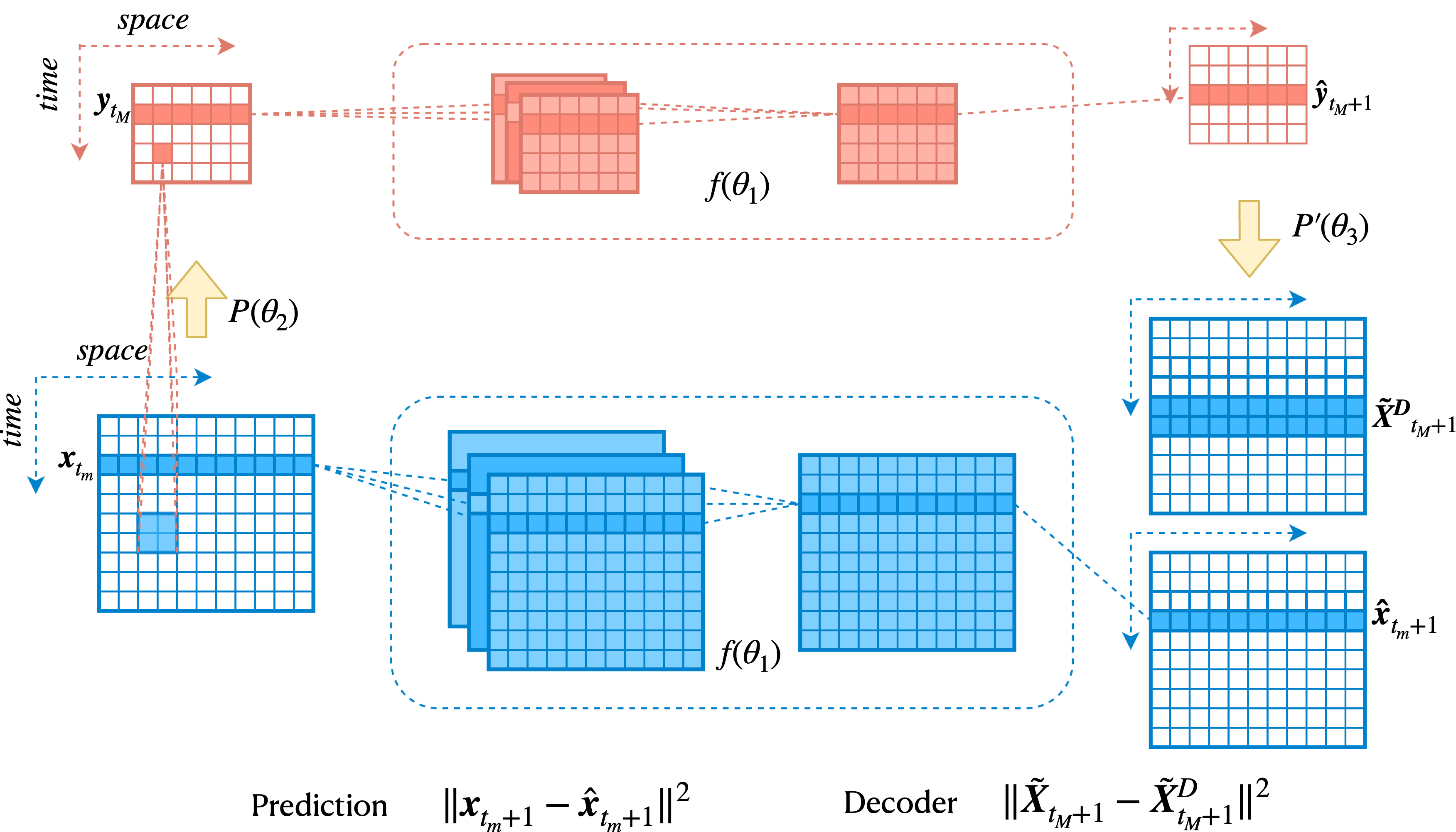
Figure 2: Framework of our model. We have two level neural network framework. The first level aims to capture the microscopic dynamics $f$ using the microstate which are presented blue in the bottom of the figure, while the second one represents the macroscopic state and dynamics $F$, which are red on the top. Both dynamics receive time-series data from their respective levels as input and produce predictions for future outcomes. As mentioned to in the main text, both the micro and macro dynamics share the same neural network structure and parameters, as depicted by $f(\theta_{1})$ in the figure. Given the discrepancy in data dimensions between the micro and macro levels—typically with macro variables being fewer — it necessitates the construction of neural networks that exhibit spatio-temporal translational invariance. A coarse-graining learner $P(\theta_{2})$,connects the two, facilitating the transformation from microscopic to macroscopic data. To prevent macrostates from falling into trivial state in the training process, we added a decoder $P(\theta_{3})$ after the macroscopic prediction. This decoder constrains its output to closely resemble the microstates. After training, the decoder can be deactivated.

3 Experiments

In the following part, we will validate the effectiveness of our frame using two examples. Cellular automata serve as a representation of deterministic dynamic systems, while diffusion dynamics stand for stochastic dynamic systems.

3.1 1d Cellular Automata

In 1D cellular automata, there are 256 different nearest-neighbor rules, which could create lots of amazing different patterns. In literature [46], the authors have summarized there are 21 rules can exhibit self-similarity through appropriate coarse-graining techniques. The coarse-graining methods in the article were found through manual search. The dynamics and evolving patterns of cellular automata correspond, so according to Eq.4 and Eq.5, a system is considered self-similar if the macroscopic patterns after coarse-graining resemble the microscopic patterns. We use the classification in this literature as the ground truth to validate the effectiveness of our framework in deterministic dynamic systems.

Dynamics Learner: We configure the dynamical learner as a 1D convolutional neural network with a kernel size of 3. Given that cellular automata operate based on nearest-neighbor interactions, a single convolutional layer is sufficient to capture the complete dynamics. We employ two kernels and combine them through a linear mapping to generate predictions for the next time step, just as Fig.2 has shown.

Coarse-Graining Learner: For the coarse-graining learner, we utilize a 2D convolutional neural network and kernel sizes of 2x2, 3x3, and 4x4 for all rules. The choice of square-shaped kernels is motivated by the need for consistency in both spatial and temporal scales after each coarse-graining step. In nearest-neighbor cellular automata, if we want the dynamics to continue to be based on nearest-neighbor interactions after coarse graining, the temporal and spatial scales should be equal, that is $S=T$. Because of the same value between $S$ and $T$, we rename them as group size $N$ for convenience in the following part.

Experiments show that we can learn the dynamics of all 256 CA rules with nearly 100 % accuracy. Rule 60 and 85 are taken as examples to show the learning result of renormalization. In the case of specifying group size, our framework can identify whether the current rule is self-similar dynamics (Fig.3). We can see that for rule 60, except group size N equals to 3, both N=2 and N=4 can map the rule to a smaller scale and keep the dynamics unchanged. And rule 85 could be renormalized as a self-dynamics only when N=3. Table 1 shows more complete results, which shows our framework can identify all the self-similar 21 rules, find the proper group size and learn coarse-grain mapping. As for non-self-similar rules, they are not fully presented here, but experiments show that they do fail self-similarity verification according to Eq. 4 and Eq. 5

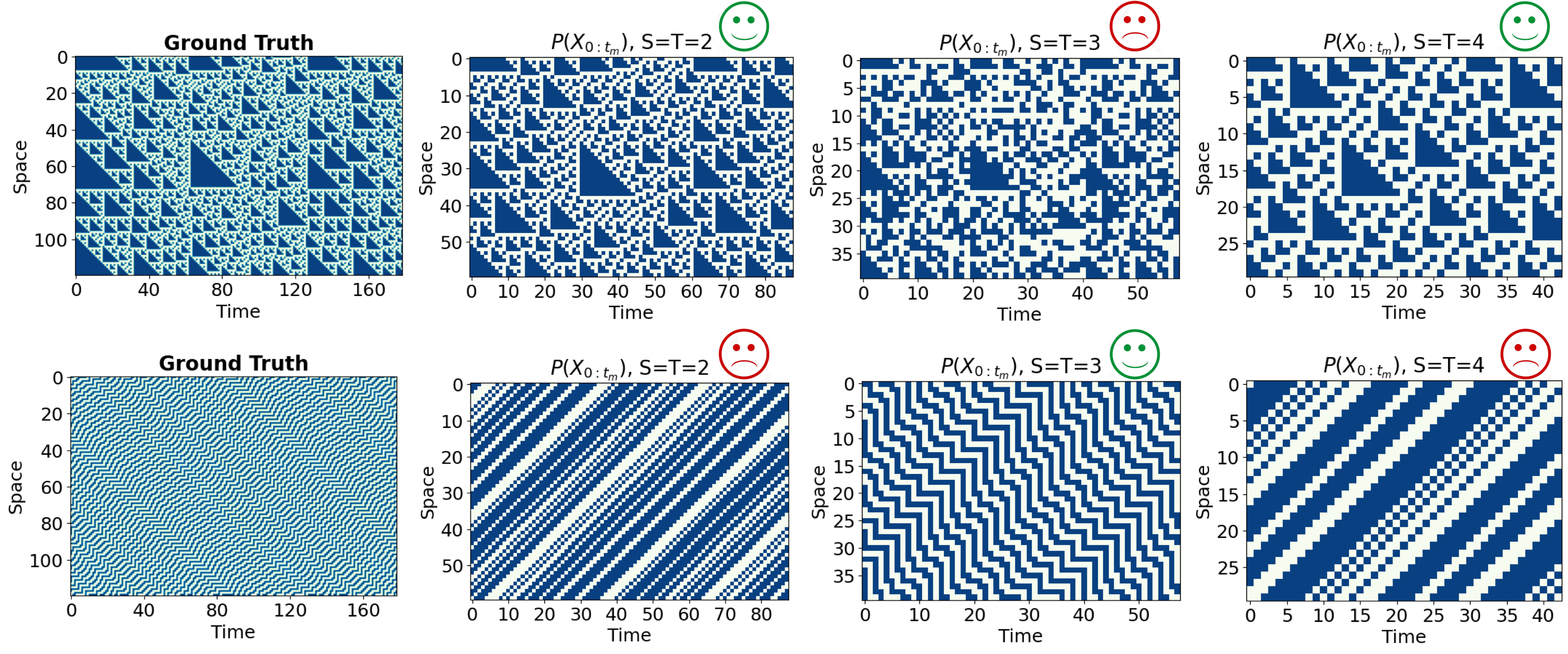
Figure 3: Examples of CA dynamic renormalization based on self-similar constraints (rule = 60 and rule = 85). The first row is the result of rule 60. They are ground truth and renormalization results of three different scales with $S=T=2,3,4$, respectively. The second row is the result of rule 85, and also are ground truth and renormalization results of three different scales with $S=T=2,3,4$. We could see except $S=T=3$, rule 60 can be renormalized as same rule in macro level, and rule 85 can be renormalized a self-similar dynamics only for $S=T=3$.

Table 1: MSE for macro prediction according the steps of self-similarity verification. Here we show applying our framework to cellular automata with all 21 self-similar rules and identifying what is the proper group size N if we want to get self similarity dynamics. The number in the table is the MSE of $\boldsymbol{y^{i}_{t+1}}$ and $(\boldsymbol{y^{i}_{t+1}})^{\prime}$ according to Eq.4 and Eq.5. 0.0 means the dynamics are self-similar.

Rule	N=2	N=3	N=4	Rule	N=2	N=3	N=4
0	0.0	0.0	0.0	170	0.0	0.0	0.0
15	0.5	0.0	0.5116	165	0.0	0.4911	0.0
51	0.5	0.0	0.5116	192	0.0	0.0	0.0
60	0.0	0.4786	0.0	195	0.0	0.4520	0.0
85	0.5	0.0	0.4884	204	0.0	0.0	0.0
90	0.0	0.5246	0.0	238	0.0	0.0	0.0
102	0.0	0.2990	0.0	240	0.0	0.0	0.0
128	0.0	0.0	0.0	252	0.0	0.0	0.0
136	0.0	0.0	0.0	254	0.0	0.0	0.0
150	0.0	0.7723	0.0	255	0.0	0.0	0.0
153	0.0	0.5407	0.0	-

3.2 Reaction-Diffusion Process

The reaction-diffusion equation is used to describe the processes of material diffusion and reaction. Typically, this equation can be used to study the distribution changes of materials over time and space. Generally speaking, the standard form of the reaction-diffusion equation is Eq.8.

$$\frac{\partial C}{\partial t}=D\frac{\partial^{2}C}{\partial x^{2}}+R(C)$$ (8)

$C(x,t)$ represents the probability distribution of particle concentration $C$ at location $x$ at time $t$. $D$ is the diffusion coefficient, and $R(C)$ is a reaction rate function related to concentration $C$, which describes the reaction process of a substance. Let us think about the simpler case, that is $R(c)=0$, which means the total concentration is conserved throughout the diffusion process. In that case, when appropriately coarse-grained, the diffusion coefficient $D$ of the diffusion process remains unchanged, indicating that the system have a self-similar dynamics. We can use this system to test whether our framework can be applied to stochastic dynamics.

Dataset: In numerical simulations of the diffusion process, it is intuitive to assume that the smaller the time interval $\Delta t$ and the spatial interval $\Delta x$, the higher accuracy of the simulation. As the intervals approach zero($\Delta t$ and $\Delta x\to 0$), the diffusion dynamics converge towards perfect self-similarty. We’ve generated data using different time-space intervals: $\Delta t=1,0.1,0.04,0.01$ and for $\Delta t\to 0$–derived from the analytical solution. All simulations evolved from $t=0$ to $t=100$ within a spatially bounded system of size 100, with periodic boundary conditions. Fig.5 (a) provides a visualization of the data.

Dynamics Learner: We modeled the dynamics using a 1D convolutional neural network (CNN). Without any prior knowledge, we experimented with different kernel sizes to assess their impact on prediction accuracy. The optimal accuracy was achieved with a kernel size of 5 (as shown in Fig.5 (c) left). A kernel size of 3 and 7, on the other hand, offered a good margin of error tolerance when $\Delta t!=0$ (Fig.5 (c) right ). In the absence of specific instructions of this paper, we standardized the kernel size to 7. Fig.5 (b) depicts the state transition vectors learned by the dynamics learner for simulation data of varying time-space interval. It’s evident that the higher the accuracy of the simulation data, the closer the dynamics transition vector is to a Gaussian distribution.

Coarse-Graining Learner: For a simple diffusion process, the relationship between particle movement in time and space satisfies $x\propto\sqrt{t}$. This means that, when renormalizing the diffusion process, the space-time scaling relationship needs to be $S\propto\sqrt{T}$ to potentially yield the same dynamics. We adopted a spatio-temporal convolutional approach for learning. Specifically, we utilized two separate 1D convolutional neural networks for time and space dimensions. By adjusting the kernel sizes for convolution and pooling, we can coarsely grain the data into a more compact space.

Firstly, we wanted to validate whether our framework could function effectively in the diffusion process. Applying the aforementioned learner to the data where $\Delta t\to 0$, Fig.4 (a) displays the visualization comparison between the ground truth and prediction result, and Fig.4 (b) show the verification of self-smilarity between $\boldsymbol{y}^{i}_{t+1}$ and $(\boldsymbol{y}^{i}_{t+1})^{\prime}$. We also calculate the relationship between the time t and the diffusion mean square distance in learned macroscopic state, and the slope of the relationship is related to the diffusion coefficient $D$. Our results show that the macroscopic and microscopic diffusion coefficients are very consistent (Fig.4 (c)), which further verifies that we have indeed learned self-similar dynamics. More quantitatively, we found that the prediction error for the dynamics could be extremely low, with an MAE approaching the magnitude of $10^{-5}$. This also passed the self-similarity test, as shown in Fig.5 (e), with errors between $\boldsymbol{y}^{i}_{t+1}$ and $(\boldsymbol{y}^{i}_{t+1})^{\prime}$ being only $3\times 10^{-4}$.

Further, by using different $\Delta t$ values as training data, we can derive various models and observe how the model outcomes differ. Fig.5 (a) illustrates the changes in the convolutional kernels learned by the dynamics as $\Delta t$ varies. We noticed that the kernels gradually converge to a bell-shaped curve. Simultaneously, the error in the dynamics decreases as $\Delta t$ diminishes, as shown in Fig.5 (b). Similarly, the error from decoder also lessens as $\Delta t$ gets smaller (in Fig.5 (c) ), with a notably pronounced advantage when learning on self-similar dynamics. This phenomenon suggests that we can not only determine the self-similarity of the dynamics we’re learning through the consistency (Fig.5 (d)), but can also judging which dynamics are closer to being self-similar based on the learning errors of both the dynamics and the decoder. Note that all experiments here are the average results of three experiments, and the error bar is not obvious in the figure due to its small value.

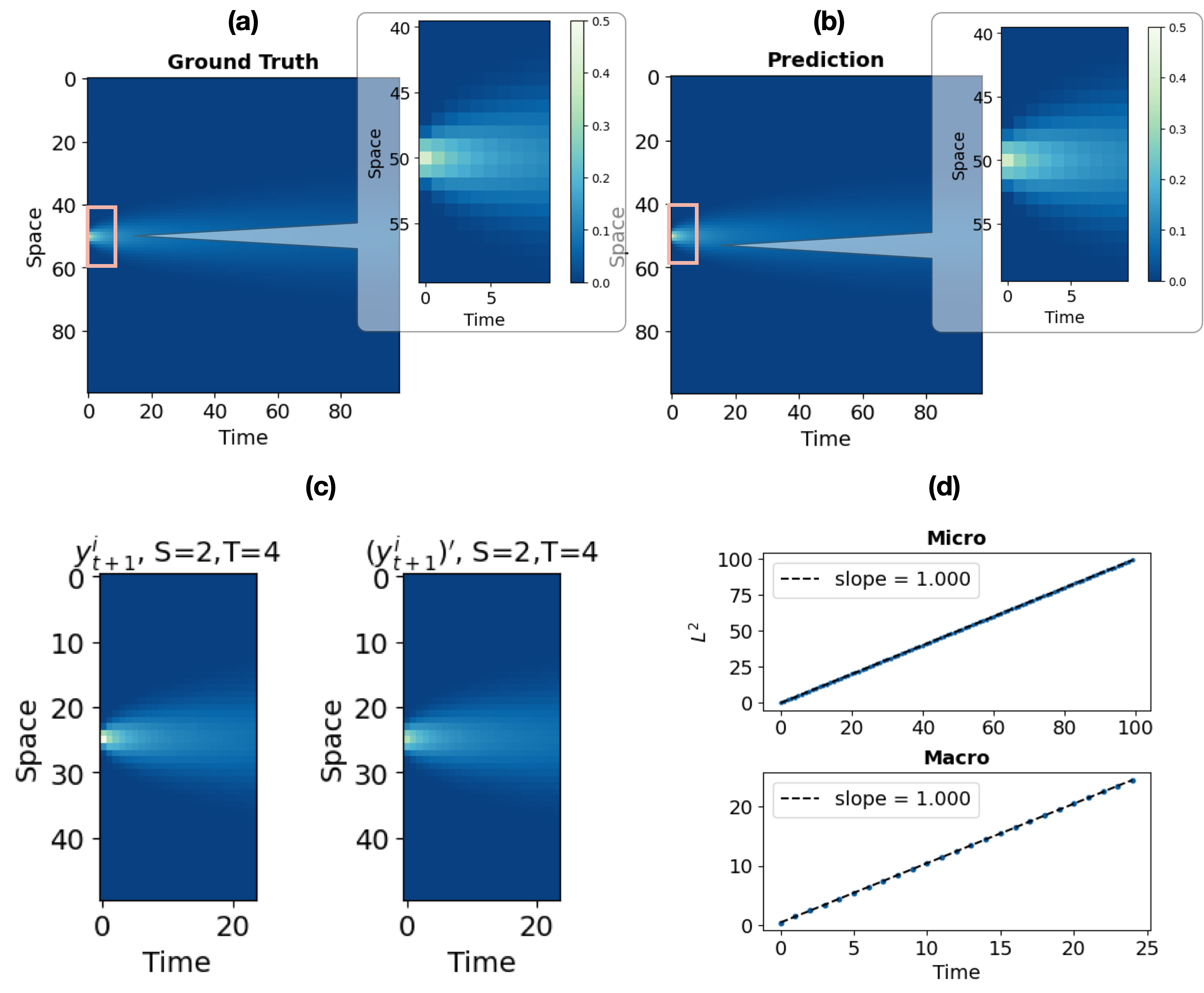
Figure 4: Results of diffusion process. (a) and (b) are ground truth and prediction of microstate, respectively. Subplots are the enlarging version of the red square in order to get more clear visualization. (c) are the verification of self-similarity, same as CA before. We set $S=2$ and $T=4$ as example, while $S=3$ and $T=9$ also have the similar results, which we don’t show here due to space constraints. (d) are the verification of the scaling relationship between time $t$ and average diffusion length $L$ in microstates and macrostates respectively.

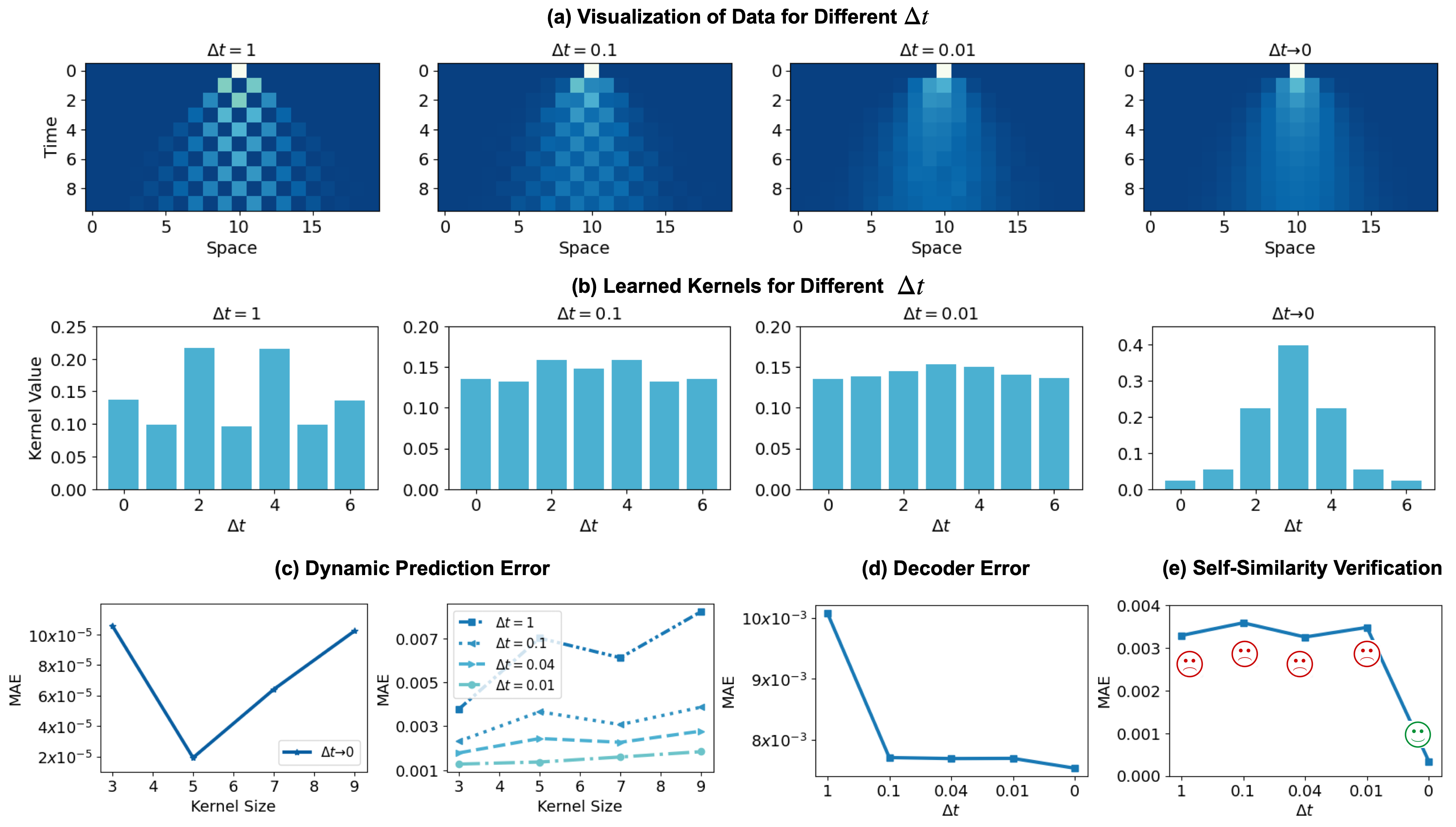
Figure 5: Comparison of different $\Delta t$ and quantitative results. (a) are the visualization of data for different $\Delta t$. (b) are the dynamic kernel learned by the dynamic learner. (c) tests the influence of different kernel sizes on dynamic accuracy. we found for the self-similar dynamic (left), kernel size = 5 and 7 could have the relative great results, while kernel size = 3 and 7 are better for none self-similar dynamic (right). So in the absence of any specific instructions, our experimental setup is kernel size = 7. (d). MAE for decoder module and the decoder error of self-similar dynamics is minimal. (e). Quantitative self-similar verification. We could found our framework is very effective for identifying self-similar dynamics.

4 Conclusion and Discussion

Analyzing complex systems from a multi-scale perspective is what sets them apart from other systems. We often find that fascinating phenomena like emergence are linked to the scale of the system. The motivation behind constructing self-similar dynamics is to find a scale-independent kernel for a dynamics system. Although our exploration is still in its early stages, our model holds significant potential.

In summary, we introduce a multiscale neural network framework that integrates self-similarity priors for modeling complex dynamic systems. We can identify if the dynamic systems are self-similar, whether deterministic or stochastic dynamics. And our framework can automatically capture scale-invariant kernel in dynamics, which means we can use fewer parameters to model the dynamic system. In our experiments, there are only a dozen of parameters in our neural model, but it also can capture the precise dynamics, as well as the reasonable renormalization strategies because of the self-similarity prior knowledge.

Renormalization signifies the alteration of models describing systems as scales vary, with dynamical renormalization focusing on the dynamical models. While physicists have historically achieved noteworthy successes with renormalization in statistical models, recent years have seen substantial progress in marrying machine learning with renormalization frameworks. However, research on dynamical renormalization has often been overly manual, necessitating the search for new appropriate renormalization strategies when faced with a novel system. Our work offers a potential framework for the fusion of dynamical renormalization with machine learning. The incorporation of self-similar prior knowledge suggests we are modeling fixed points in the dynamical parameter space. We firmly believe that data-driven multi-scale modeling approaches will present viable solutions for automating dynamical renormalization, paving a significant avenue for the integration of machine learning and statistical physics.

5 Acknowledgement

We would like to express our gratitude to Swarma Club for their support towards our paper, as well as the constructive discussions contributed by Zhangzhang, Mingzhe Yang, Zhongpu Qiu, Mingze Qi. During the preparation of this work the author(s) used GPT-4 in the process of writing paper in order to make the English expression more accuracy and fluency. After using this tool/service, the author(s) reviewed and edited the content as needed and take(s) full responsibility for the content of the publication.

References

- [1] Franziska Taubert, Rico Fischer, Jürgen Groeneveld, Sebastian Lehmann, Michael S Müller, Edna Rödig, Thorsten Wiegand, and Andreas Huth. Global patterns of tropical forest fragmentation. Nature, 554(7693):519–522, 2018.
- [2] Ole Peters and J. David Neelin. Critical phenomena in atmospheric precipitation. Nature Physics, 2(6):393–396, 2006.
- [3] Reginald D Smith. The dynamics of internet traffic: self-similarity, self-organization, and complex phenomena. Advances in Complex Systems, 14(06):905–949, 2011.
- [4] Daniele Notarmuzi, Claudio Castellano, Alessandro Flammini, Dario Mazzilli, and Filippo Radicchi. 01Universality, criticality and complexity of information propagation in social media. Nature Communications, (2022):1–8, 2021.
- [5] Suzana Herculano-Houzel, Paul R. Manger, and Jon H. Kaas. Brain scaling in mammalian evolution as a consequence of concerted and mosaic changes in numbers of neurons and average neuronal cell size. Frontiers in Neuroanatomy, 8(AUG):1–28, 2014.
- [6] Daria La Rocca, Nicolas Zilber, Patrice Abry, Virginie van Wassenhove, and Philippe Ciuciu. Self-similarity and multifractality in human brain activity: A wavelet-based analysis of scale-free brain dynamics. Journal of Neuroscience Methods, 309(April):175–187, 2018.
- [7] Tiago L. Ribeiro, Dante R. Chialvo, and Dietmar Plenz. Scale-Free Dynamics in Animal Groups and Brain Networks. Frontiers in Systems Neuroscience, 14(January):1–10, 2021.
- [8] George F. Grosu, Alexander V. Hopp, Vasile V. Moca, Harald Bârzan, Andrei Ciuparu, Maria Ercsey-Ravasz, Mathias Winkel, Helmut Linde, and Raul C. Mureşan. The fractal brain: scale-invariance in structure and dynamics. Cerebral Cortex, 33(8):4574–4605, 2023.
- [9] Chaoming Song and Shlomo Havlin. Self-similarity of complex networks. Nature, 433(January):2–5, 2005.
- [10] Filippo Radicchi, José J. Ramasco, Alain Barrat, and Santo Fortunato. Complex networks renormalization: Flows and fixed points. Physical Review Letters, 101(14):3–6, 2008.
- [11] Filippo Radicchi, Alain Barrat, Santo Fortunato, and José J. Ramasco. Renormalization flows in complex networks. Physical Review E, 79(2):1–11, 2009.
- [12] Hernán D. Rozenfeld, Chaoming Song, and Hernán A. Makse. Small-world to fractal transition in complex networks: A renormalization group approach. Physical Review Letters, 104(2):1–4, 2010.
- [13] Guillermo García-Pérez, Marián Boguñá, and M. Ángeles Serrano. Multiscale unfolding of real networks by geometric renormalization. Nature Physics, 14(6):583–589, 2018.
- [14] Dan Chen, Housheng Su, Xiaofan Wang, Gui Jun Pan, and Guanrong Chen. Finite-size scaling of geometric renormalization flows in complex networks. Physical Review E, 104(3):1–12, 2021.
- [15] Dan Chen, Housheng Su, and Zhigang Zeng. Geometric Renormalization Reveals the Self-Similarity of Weighted Networks. IEEE Transactions on Computational Social Systems, 10(2):426–434, 2023.
- [16] Pablo Villegas, Tommaso Gili, Guido Caldarelli, and Andrea Gabrielli. Laplacian renormalization group for heterogeneous networks. Nature Physics, 19(3):445–450, 2023.
- [17] A. C. Antoulas. Approximation of large-scale dynamical systems: An overview. IFAC Proceedings Volumes (IFAC-PapersOnline), 37(11):19–28, 2004.
- [18] Brian Munsky and Mustafa Khammash. The finite state projection approach for the analysis of stochastic noise in gene networks. IEEE Transactions on Automatic Control, 53(SPECIAL ISSUE):201–214, 2008.
- [19] Leo P Kadanoff. Scaling laws for ising models near tc. Physics Physique Fizika, 2(6):263, 1966.
- [20] Kenneth G Wilson. The renormalization group and critical phenomena. Reviews of Modern Physics, 55(3):583, 1983.
- [21] Andrea Pelissetto and Ettore Vicari. Critical phenomena and renormalization-group theory. Physics Reports, 368(6):549–727, 2002.
- [22] Ulrich Schollwöck. The density-matrix renormalization group. Reviews of modern physics, 77(1):259, 2005.
- [23] Tauber. critical dynamics. 2014.
- [24] Andrea Cavagna, Daniele Conti, Chiara Creato, Lorenzo Del Castello, Irene Giardina, Tomas S. Grigera, Stefania Melillo, Leonardo Parisi, and Massimiliano Viale. Dynamic scaling in natural swarms. Nature Physics, 13(9):914–918, 2017.
- [25] M. C. Yalabik and J. D. Gunton. Monte Carlo renornnlization-group studies of kinetic Ising models. Physical Review B, 25(1):2–5, 1982.
- [26] Gene F Mazenko, Jorge E Hirsch, and J Nolan. Real-space dynamic renormalization group. III. Calculation of correlation functions. 23(3):1431–1446, 1981.
- [27] Alessandro Vespignani, Stefano Zapperi, and Pietronero Luciano. 22Renormalization approach to the self-organized critical behavior of sandpile models. Physical Review E, 2(2):243–253, 1995.
- [28] Eugene V. Ivashkevich, Alexander M. Povolotsky, Alessandro Vespignani, and Stefano Zapperi. 22Dynamical real space renormalization group applied to sandpile models. Physical Review E - Statistical Physics, Plasmas, Fluids, and Related Interdisciplinary Topics, 60(2):1239–1251, 1999.
- [29] Chai Yu Lin and Chin Kun Hu. Renormalization-group approach to an Abelian sandpile model on planar lattices. Physical Review E - Statistical Physics, Plasmas, Fluids, and Related Interdisciplinary Topics, 66(2):1–29, 2002.
- [30] Andrea Cavagna, Luca Di Carlo, Irene Giardina, Luca Grandinetti, Tomas S. Grigera, and Giulia Pisegna. 22Dynamical Renormalization Group Approach to the Collective Behavior of Swarms. Physical Review Letters, 123(26):268001, 2019.
- [31] Andrea Cavagna, Luca Di Carlo, Irene Giardina, Luca Grandinetti, Tomas S. Grigera, and Giulia Pisegna. 22Renormalization group crossover in the critical dynamics of field theories with mode coupling terms. Physical Review E, 100(6):1–29, 2019.
- [32] A. Cavagna, P. M. Chaikin, D. Levine, S. Martiniani, A. Puglisi, and M. Viale. Vicsek model by time-interlaced compression: A dynamical computable information density. Physical Review E, 103(6):1–10, 2021.
- [33] George Em Karniadakis, Ioannis G. Kevrekidis, Lu Lu, Paris Perdikaris, Sifan Wang, and Liu Yang. 31.Physics-informed machine learning. Nature Reviews Physics, 3(6):422–440, 2021.
- [34] Logan G. Wright, Tatsuhiro Onodera, Martin M. Stein, Tianyu Wang, Darren T. Schachter, Zoey Hu, and Peter L. McMahon. Deep physical neural networks trained with backpropagation. Nature, 601(7894):549–555, 2022.
- [35] Ricardo Vinuesa and Steven L. Brunton. Enhancing computational fluid dynamics with machine learning. Nature Computational Science, 2(6):358–366, 2022.
- [36] Nicholas Walker, Ka Ming Tam, and Mark Jarrell. Deep learning on the 2-dimensional Ising model to extract the crossover region with a variational autoencoder. Scientific Reports, 10(1):1–12, 2020.
- [37] Kenta Shiina, Hiroyuki Mori, Yusuke Tomita, Hwee Kuan Lee, and Yutaka Okabe. Inverse renormalization group based on image super-resolution using deep convolutional networks. Scientific Reports, 11(1):1–9, 2021.
- [38] Hong Ye Hu, Shuo Hui Li, Lei Wang, and Yi Zhuang You. Machine learning holographic mapping by neural network renormalization group. Physical Review Research, 2(2):23369, 2020.
- [39] Wanda Hou and Yi-Zhuang You. Machine Learning Renormalization Group for Statistical Physics. arXiv preprint, pages 1–13, 2023.
- [40] Dorit Ron, Achi Brandt, and Robert H. Swendsen. Monte Carlo renormalization-group calculation for the d=3 Ising model using a modified transformation. Physical Review E, 104(2), 2021.
- [41] Jui Hui Chung and Ying Jer Kao. Neural Monte Carlo renormalization group. Physical Review Research, 3(2), 2021.
- [42] Shuo Hui Li and Lei Wang. Neural Network Renormalization Group. Physical Review Letters, 121(26):1–10, 2018.
- [43] Patrick M. Lenggenhager, Doruk Efe Gökmen, Zohar Ringel, Sebastian D. Huber, and MacIej Koch-Janusz. Optimal renormalization group transformation from information theory. Physical Review X, 10(1):11037, 2020.
- [44] Satoshi Iso, Shotaro Shiba, and Sumito Yokoo. Scale-invariant feature extraction of neural network and renormalization group flow. Physical Review E, 97(5):1–16, 2018.
- [45] Jiang Zhang and Kaiwei Liu. Neural information squeezer for causal emergence. Entropy, 25(1):26, 2022.
- [46] Navot Israeli and Nigel Goldenfeld. Coarse-graining of cellular automata, emergence, and the predictability of complex systems. Physical Review E - Statistical, Nonlinear, and Soft Matter Physics, 73(2):1–17, 2006.