Lag-Llama: Towards Foundation Models for Probabilistic Time Series Forecasting

Abstract

Over the past years, foundation models have caused a paradigm shift in machine learning due to their unprecedented capabilities for zero-shot and few-shot generalization. However, despite the success of foundation models in modalities such as natural language processing and computer vision, the development of foundation models for time series forecasting has lagged behind. We present Lag-Llama, a general-purpose foundation model for univariate probabilistic time series forecasting based on a decoder-only transformer architecture that uses lags as covariates. Lag-Llama is pretrained on a large corpus of diverse time series data from several domains, and demonstrates strong zero-shot generalization capabilities compared to a wide range of forecasting models on downstream datasets across domains. Moreover, when fine-tuned on relatively small fractions of such previously unseen datasets, Lag-Llama achieves state-of-the-art performance, outperforming prior deep learning approaches, emerging as the best general-purpose model on average. Lag-Llama serves as a strong contender to the current state-of-art in time series forecasting and paves the way for future advancements in foundation models tailored to time series data.

1 Introduction

Probabilistic time series forecasting is an important practical problem arising in a wide range of applications, from finance and weather forecasting to brain imaging and computer systems performance management (Peterson, 2017). Accurate probabilistic forecasting is usually an essential step towards the subsequent decision-making in such practical domains. The probabilistic nature of such forecasting endows decision-makers with a notion of uncertainty, allowing them to consider a variety of future scenarios, along with their respective likelihoods. Various methods have been proposed for this task, ranging from classical autoregressive models (Hyndman & Athanasopoulos, 2021) to the more recent neural forecasting methods based on deep learning architectures (Torres et al., 2021). Note that the overwhelming majority of these previous approaches are focused on building dataset-specific models, i.e. models tested on the same dataset in which training is performed.

Recently, however, machine learning is witnessing a paradigm shift due to the rise of foundation models (Bommasani et al., 2022) — large-scale, general-purpose neural networks pretrained in an unsupervised manner on large amounts of diverse data across various data distributions. Such models demonstrate remarkable few-shot generalization capabilities on a wide range of downstream datasets (Brown et al., 2020a), often outperforming dataset-specific models. Following the successes of foundation models in language and image processing domains(OpenAI, 2023; Radford et al., 2021), we aim to develop foundation models for time series, investigate their behaviour at scale, and push the limits of transfer achievable across diverse time series domains.

In this paper, we present Lag-Llama— a foundation model for probabilistic time series forecasting trained on a large collection of open time series data, and evaluated on unseen time series datasets. We investigate the performance of Lag-Llama across several settings where unseen time series datasets are encountered downstream with different levels of data history being available, and show that Lag-Llama performs comparably or better against state-of-the-art dataset-specific models.

Our contributions:

• We present Lag-Llama, a foundation model for univariate probabilistic time series forecasting based on a simple decoder-only transformer architecture that uses lags as covariates.

• We show that Lag-Llama, when pretrained from scratch on a broad, diverse corpus of datasets, has strong zero-shot performance on unseen datasets, and performs comparably to models trained on the specific datasets.

• Lag-Llama also demonstrates state-of-the-art performance across diverse datasets from different domains after finetuning, and emerges as the best general-purpose model without any knowledge of downstream datasets.

• We demonstrate the strong few-shot adaptation performance of Lag-Llama on previously unseen datasets, across varying fractions of data history being available.

• We investigate the diversity of the pretraining corpus used to train Lag-Llama, and present the scaling laws of Lag-Llama with respect to the pretraining data.

2 Related Work

Statistical models have been the cornerstone of time series forecasting for decades, evolving continuously to address complex forecasting challenges. Traditional models such as ARIMA (Autoregressive Integrated Moving Average) set the foundation by using autocorrelation to forecast future values. ETS (Error, Trend, Seasonality) models advanced this by decomposing a time series into its fundamental components, allowing for more nuanced forecasting that captures trends and seasonal patterns. Theta models, introduced by Assimakopoulos & Nikolopoulos (2000), represented another significant advancement in time series forecasting. By applying a decomposition technique combining both long-term trend and seasonality, these models offer a simple yet effective method for forecasting Despite the success of the considerable successes of these statistical models and more advanced ones (Croston, 1972; Syntetos & Boylan, 2005; Hyndman & Athanasopoulos, 2018), these models share common limitations. Their primary shortfall lies in their inherent assumption of linear relationships and stationarity in time series data, which is often not the case in real-world scenarios marked by abrupt changes and non-linear dynamics. Furthermore, they may require extensive manual tuning and domain knowledge to select appropriate models and parameters for specific forecasting tasks.

Neural forecasting is a rapidly developing research area following the explosion of machine learning (Benidis et al., 2022). Various architectures have been developed for this setting, starting with RNN-based and LSTM-based models (Salinas et al., 2020; Wen et al., 2018). More recently in light of the recent success of transformers (Vaswani et al., 2017) for sequence-to-sequence modelling for natural language processing, many variations of transformers have been proposed for time series forecasting. Different models (Nie et al., 2023a; Wu et al., 2020a, b) process the input time series in different ways to be digestible by a vanilla transformer, then re-process the output of a transformer for a point forecast or a probabilistic forecast. On the other hand, various other works propose alternative strategies to vanilla attention and build off the transformer architecture, for better models tailored for time series (Lim et al., 2021; Li et al., 2023; Ashok et al., 2023; Oreshkin et al., 2020a; Zhou et al., 2021a; Wu et al., 2021; Woo et al., 2023; Liu et al., 2022b; Zhou et al., 2022; Liu et al., 2022a; Ni et al., 2023; Li et al., 2019; Gulati et al., 2020).

Foundation models are an emerging paradigm of self-supervised (or) unsupervised learning on large datasets (Bommasani et al., 2022). Many such models (Devlin et al., 2019; OpenAI, 2023; Chowdhery et al., 2022; Radford et al., 2021; Wang et al., 2022) have demonstrated adaptability across modalities, extending beyond web data to scientific domains such as protein design (Robert Verkuil, 2022). Scaling the model, dataset size and data diversity have also been shown to result in remarkable transfer capabilities and excellent few-shot learning on novel datasets and tasks (Thrun & Pratt, 1998; Brown et al., 2020b). Self-supervised learning techniques have also been proposed for time series (Li et al., 2023; Woo et al., 2022a; Yeh et al., 2023). Most related to our work is Yeh et al. (2023) who train on a corpus of time series datasets. The key difference is that they validate their model only on the downstream classification tasks, and do not validate on forecasting tasks. Works such as Time-LLM (Jin et al., 2023), LLM4TS (Chang et al., 2023), GPT2(6) (Zhou et al., 2023a), UniTime (Liu et al., 2023), and TEMPO (Anonymous, 2024) freeze LLM encoder backbones while simultaneously fine-tuning/adapting the input and distribution heads for forecasting. The main goal of our work is to apply the foundation model approach to time series data and to investigate the extent of the transfer achievable across a wide range of time series domains.

3 Probabilistic Time Series Forecasting

We consider a dataset of $D\geq 1$ univariate time series, $\mathcal{D}_{\mathrm{train}}=\{x_{1:T^{i}}^{i}\}_{i=1}^{D}$ sampled at a specific discrete set of time points $t\in\{1,\ldots,T^{i}\}$ where $T^{i}$ represents the length of the time series $i$. Given this dataset, we aim to train a predictive model that can accurately predict the values at the future $P\geq 1$ time points; we refer to these timesteps of our $D$ time series as to the test dataset, denoted $\mathcal{D}_{\mathrm{test}}=\{x_{T^{i}+1:T^{i}+P}^{i}\}_{i=1}^{D}$.

The univariate probabilistic time series forecasting problem involves modelling an unknown joint distribution of the $P$ future values of a one-dimensional sequence given its observed past until timestep $t$ from which prediction should be performed, and covariates:

$$p_{\mathcal{\phi}}(x_{t+1:t+P}^{i}\mid x_{1:t}^{i},\mathbf{c}^{i}_{1:t+P}).$$ (1)

where $\mathcal{\phi}$ represents the parameters of a parametric distribution. In practice, rather than considering the whole history of each time series $i$, which can vary considerably, we can instead sub-sample fixed context windows of size $C\geq 1$ of our choosing from the complete time series and learn an approximation of the unknown distribution of the next $P$ future values given the covariates:

$$p_{\mathcal{\phi}}(x_{C+1:C+P}^{i}\mid x_{1:C}^{i},\mathbf{c}^{i}_{1:C+P}).$$ (2)

When the distribution is modeled by a neural network with parameters $\theta$, predictions are then conditioned on these (learned) parameters $\theta$. We will approximate the distribution in Eq. 2 by an autoregressive model, using the chain rule of probability as follows:

$$p_{\mathcal{\phi}}(x_{C+1:C+P}^{i}\mid x_{1:C}^{i},\mathbf{c}^{i}_{1:C+P};\theta)=\\ \prod_{t=C+1}^{C+P}p_{\mathcal{\phi}}(x_{t}^{i}\mid x_{1:t-1}^{i},\mathbf{c}^{i}_{1:t-1};\theta).$$

4 Lag-Llama

We present Lag-Llama, a foundation model for univariate probabilistic forecasting. The first step in building such a foundation model for time series is training on a large corpus of diverse time series. When training on heterogenous univariate time series corpora, the frequency of the time series in our corpus varies. Further, when adapting our foundation model to downstream datasets, we may encounter new frequencies and combinations of seen frequencies, which our model should be capable of handling. We now present a general method for tokenizing series from such a dataset, without directly relying on the frequency of any specific dataset, and thus potentially allowing unseen frequencies and combinations of seen frequencies to be used at test time.

4.1 Tokenization: Lag Features

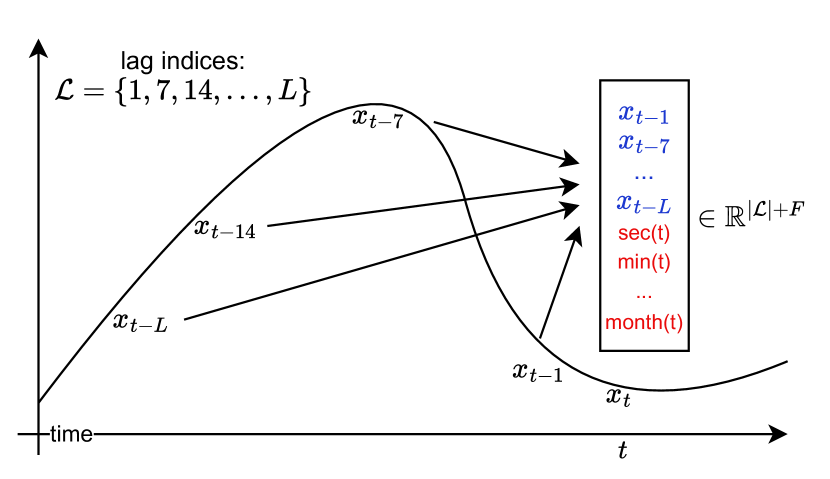
Figure 1: For a time series, we depict the tokenization at the timestep $t$ of the value $x_{t}$ which contains lag features constructed using an example set of lag indices $\mathcal{L}$, where each value in the vector is from the past of $x_{t}$ (in blue), and $F$ possible temporal covariates (date-time features) constructed from timestamp $t$ (red).

The tokenization scheme of Lag-Llama involves constructing lagged features from the prior values of the time series, constructed according to a specified set of appropriate lag indices that include quarterly, monthly, weekly, daily, hourly, and second-level frequencies. Given a sorted set of positive lag indices $\mathcal{L}=\{1,\ldots,L\}$, we define the lag operation on a particular time value as $x_{t}\mapsto\mathbf{k}_{t}\in\mathbb{R}^{|\mathcal{L}|}$ where each entry $j$ of $\mathbf{k}_{t}$ is given by $\mathbf{k}_{t}[j]=x_{t-\mathcal{L}[j]}$. Thus to create lag features for some context-length window $x_{1:C}$ we need to sample a larger window with $L$ more historical points denoted by $x_{-L:C}$. In addition to these lagged features, we add date-time features of all the frequencies in our corpus, namely second-of-minute, hour-of-day, etc. up till the quarter-of-year from the time index $t$. Note that while the primary goal of these date-time features is to provide additional information, for any time series, all except one date-time feature will remain constant from one time-step to the next, and from the model can implicitly make sense of the frequency of the time series as well. Assuming we employ a total of $F$ date-time features, each of our tokens is of size $|\mathcal{L}|+F$. Fig. 1 shows an example tokenization. We note that a downside to using lagged features in tokenization is that it requires an $L$-sized or larger context window.

4.2 Lag-Llama Architecture

Lag-Llama’s architecture is based on the decoder-only transformer-based architecture LLaMA (Touvron et al., 2023).

Fig. 2 shows a general schematic of this model with $M$ decoder layers. A univariate sequence of length $x^{i}_{-L:C}$ along with its covariates is tokenized by concatenating the covariate vectors to a sequence of $C$ tokens $\mathbf{x}^{i}_{1:C}$. These tokens are passed through a shared linear projection layer that maps the features to the hidden dimension of the attention module. Similar to in Touvron et al. (2023), Lag-Llama incorporates pre-normalization via the RMSNorm (Zhang & Sennrich, 2019) and Rotary Positional Encoding (RoPE) (Su et al., 2021) at each attention layer’s query and key representations as in LLaMA (Touvron et al., 2023).

After passing through the causally masked transformer layers, the model predicts the parameters $\phi$ of the forecast distribution of the next timestep, where the parameters are output by a parametric distribution head, as described in Sec. 4.3. The negative log-likelihood of the predicted distribution of all predicted timesteps is minimized.

At inference time, given a time series of size at least $L$, we can construct a feature vector that is passed to the model to obtain the distribution of the next time point. In this fashion, via greedy autoregressive decoding, we can obtain many simulated trajectories of the future up to our chosen prediction horizon $P\geq 1$. From these empirical samples, we can calculate the uncertainty intervals for downstream decision-making tasks and metrics with respect to held-out data.

4.3 Choice of Distribution Head

The last layer of Lag-Llama is a distinct layer known as the distribution head, which projects the model’s features to the parameters of a probability distribution. We can combine different distribution heads with the representational capacity of the model to output the parameters $\phi$ of any parametric probability distribution. For our experiments, we adopt a Student’s $t$-distribution (Student, 1908) and output the three parameters corresponding to this distribution, namely its degrees of freedom, mean, and scale, with appropriate non-linearities to ensure the appropriate parameters stay positive. More expressive choices of distributions, such as normalizing flows (Rasul et al., 2021b) and copulas (Salinas et al., 2019a; Drouin et al., 2022; Ashok et al., 2023) are potential choices of distribution heads, however with the potential overhead of difficulties in model training and optimization. The goal of our work was to keep the model as simple as possible, which led us to adopt a simple parametric distributional head. We leave the exploration of such distribution heads for future work.

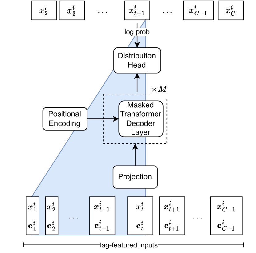
Figure 2: The Lag-Llama architecture. Lag-Llama learns to output a distribution over the values of the next time step based on lagged input features. The input to the model is the token of a univariate time series $i$ at a given timestep, $\mathbf{x}^{i}_{t}$, constructed as described in Sec.4.1. Here, we use $\mathbf{c}_{t}^{i}$ to refer to all additional covariates used along with the value at a timestep $t$, which include the $|\mathcal{L}|$ lags, $F$ date-time features, and summary statistics. The inputs are projected through $M$ masked decoder layers. The features are then passed through the distribution head and trained to predict the parameters of the forecast distribution of the next timestep.

4.4 Value Scaling

When training on a large corpus of time series data from different datasets and domains, each time series can be of different numerical magnitude. Since we pretrain a foundation model over such data, we utilize the scaling heuristic (Salinas et al., 2019b) where for each univariate window, we calculate its mean value $\mu^{i}=\sum_{t=1}^{C}x^{i}_{t}/C$ and variance $\sigma^{i}$. We can then replace the time series $x^{i}_{1:C}$ in the window by $\{(x^{i}_{t}-\mu^{i})/\sigma^{i}\}_{t=1}^{C}$. We also incorporate $\mu^{i}$ and $\sigma^{i}$ as time independent real-valued covariates for each token, to give the model information of the statistics of the inputs, which we call summary statistics.

During training and obtaining likelihood, the values are transformed using the mean and variance, while sampling, every timestep of data that is sampled is de-standardized using the same mean and variance. In practice, instead of the standard scaler, we find the following standardization strategy works well when pretraining our model.

Robust Standardization ensures that our time series processing is robust to outliers. This procedures normalizes the series by removing the median and scaling according to the Interquartile Range (IQR) (Dekking et al., 2005). For a context-window sized series $x_{1:C}=\{x_{1},x_{2},...,x_{C}\}$ we standardize each time point as:

$$x^{\prime}_{t} =\frac{x_{t}-\operatorname{Med}(x_{1:C})}{\operatorname{IQR}(x_{1:C})},\quad\textrm{where}$$ (3)

$$\operatorname{IQR}(x_{1:C}) =\operatorname{Med}(\{x_{\lceil C/2\rceil:C}\})-\operatorname{Med}(\{x_{1:\lfloor C/2\rfloor}\}).$$ (4)

4.5 Training Strategies

We employ a series of training strategies to effectively pretrain Lag-Llama on the corpus of datasets. Firstly, we find that employing a stratified sampling approach where the datasets in the corpus are weighed by the amount of total number of series is useful when sampling random windows from the pretraining corpus. Further, we find that employing time series augmentation techniques of Freq-Mix and Freq-Mask (Chen et al., 2023) serve useful to reduce overfitting. We search the hyperparameters of these augmentation strategies as part of our hyperparameter search.

5 Experimental Setup

5.1 Datasets

We collate a diverse corpus of $27$ time series datasets from several sources across six different semantically grouped domains such as energy, transportation, economics, nature, air quality and cloud operations; each dataset has a different set of characteristics, such as prediction lengths, number of series, lengths of each series, and frequencies.

We leave out a few datasets from each domain for testing the few-shot generalization abilities of the pretrained model, whle using the remaining datasets for pretraining the foundation model. Furthermore, we set aside datasets from entirely different domains to assess our model’s performance on data that may lack any potential similarity to the datasets in pretraining. Such a setup mimics the real-world use of our model, where one may adapt it for datasets that fall closely within the distribution of domains that the model has been trained on, as well as datasets in completely different domains. Our pretraining corpus comprises a total of $7,965$ different univariate time series, each of different lengths, when put together, comprising a total of around $352$ million data windows (tokens) for our model to train on. App. § A lists the datasets we use, along with their sources and properties, their respective domains, and the dataset split used in our experiments.

Note that the term “domain” used here is just a label used to group several datasets, which does not represent a common source or data distribution; each of the pretraining and test datasets possesses very different general characteristics (patterns, seasonalities), apart from having other distinct properties. We use the default prediction length of each dataset for evaluation and ensure that there is a wide variety of prediction horizons in our unseen corpus of datasets, to evaluate models on short-term, medium-term, and long-term forecasting setups. App. § A lists the different datasets used in this work, along with the sources and properties of each dataset. Sec. § 7.1 analyses the diversity of our corpus of datasets.

Table 1: CRPS of Lag-Llama zero-shot and on finetuning on the unseen datasets, compared to supervised baselines trained solely on the respective datasets. Lower is better. A mean or standard deviation of 0.0000 signifies that the first non-zero digit is beyond $3$ decimal places. The best results are in bold, and the second best results are in brown.

Model	Dataset							Average Rank
	weather	ped-counts	ett-m2	platform-delay	requests	beijing-pm2.5	exchange
Supervised
ETSFormer	0.528$\pm$0.175	0.275$\pm$0.024	0.140$\pm$0.002	0.171$\pm$0.025	0.218$\pm$0.070	0.266$\pm$0.099	0.029$\pm$0.014	13.000
NPTS	0.276$\pm$0.000	0.684$\pm$0.006	0.139$\pm$0.000	0.132$\pm$0.001	0.085$\pm$0.001	0.170$\pm$0.003	0.059$\pm$0.001	12.714
OFA	0.265$\pm$0.006	0.605$\pm$0.023	0.130$\pm$0.006	0.213$\pm$0.011	0.121$\pm$0.011	0.130$\pm$0.009	0.015$\pm$0.001	11.357
AutoFormer	0.240$\pm$0.021	0.247$\pm$0.011	0.088$\pm$0.014	0.152$\pm$0.030	0.301$\pm$0.178	0.151$\pm$0.002	0.037$\pm$0.025	11.000
CrostonSBA	0.177$\pm$0.000	0.594$\pm$0.000	0.102$\pm$0.000	0.097$\pm$0.000	0.042$\pm$0.000	0.198$\pm$0.000	0.031$\pm$0.000	9.429
AutoARIMA	0.213$\pm$0.000	0.755$\pm$0.000	nan$\pm$nan	0.112$\pm$0.000	0.076$\pm$0.000	0.110$\pm$0.000	0.009$\pm$0.000	8.333
AutoETS	0.215$\pm$0.000	0.625$\pm$0.000	0.081$\pm$0.000	0.297$\pm$0.000	0.041$\pm$0.000	0.090$\pm$0.000	0.008$\pm$0.000	8.000
DynOptTheta	0.217$\pm$0.000	1.817$\pm$0.000	0.049$\pm$0.000	0.118$\pm$0.000	0.055$\pm$0.000	0.108$\pm$0.000	0.008$\pm$0.000	7.857
Informer	0.172$\pm$0.011	0.223$\pm$0.005	0.070$\pm$0.003	0.106$\pm$0.009	0.104$\pm$0.012	0.057$\pm$0.003	0.017$\pm$0.004	6.429
DeepAR	0.148$\pm$0.004	0.239$\pm$0.002	0.068$\pm$0.003	0.068$\pm$0.003	0.045$\pm$0.009	0.154$\pm$0.000	0.012$\pm$0.000	5.714
PatchTST	0.178$\pm$0.013	0.254$\pm$0.001	0.035$\pm$0.000	0.094$\pm$0.001	0.024$\pm$0.003	0.145$\pm$0.001	0.011$\pm$0.000	5.643
N-BEATS	0.134$\pm$0.003	0.267$\pm$0.018	0.031$\pm$0.005	0.112$\pm$0.007	0.021$\pm$0.005	0.081$\pm$0.004	0.024$\pm$0.004	5.071
TFT	0.151$\pm$0.016	0.268$\pm$0.009	0.030$\pm$0.000	0.099$\pm$0.001	0.015$\pm$0.003	0.156$\pm$0.000	0.008$\pm$0.000	5.000
Zero-shot
Lag-Llama	0.164$\pm$0.001	0.285$\pm$0.033	0.063$\pm$0.002	0.091$\pm$0.002	0.090$\pm$0.015	0.130$\pm$0.009	0.011$\pm$0.001	6.714
Finetuned
Lag-Llama	0.132$\pm$0.001	0.227$\pm$0.010	0.017$\pm$0.001	0.096$\pm$0.002	0.012$\pm$0.002	0.125$\pm$0.021	0.009$\pm$0.000	2.786

5.2 Baselines

We compare the performance of Lag-Llama to that of a large set of baselines, including both standard statistical models, as well as deep neural networks.

Through AutoGluon (Shchur et al., 2023), an AutoML framework for probabilistic time series forecasting, we benchmark against $5$ well-known statistical time series forecasting models: AutoARIMA (Hyndman & Khandakar, 2008) and AutoETS (Hyndman & Khandakar, 2008) which are established statistical models that tune model parameters locally for each time series (Hyndman & Khandakar, 2008), CrostonSBA (Syntetos and Boylan Approximate) (Croston, 1972; Syntetos & Boylan, 2005) an intermittent demand forecasting model using Croston’s model with the Syntetos-Boylan bias correction approach, DynOptTheta (The Dynamically Optimized Theta model) (Box & Jenkins, 1976) a statistical forecasting method that is based on the decomposition of the time series into trend, seasonality and noise, and NPTS (Non-Parametric Time Series Forecaster) (Shchur et al., 2023), a local forecasting method that assumes a non-parametric sampling distribution. We further compare with $3$ strong deep-learning methods through the same AutoGluon framework: DeepAR (Salinas et al., 2020), an autoregressive RNN-based method that has been shown to be a strong contender for probabilistic forecasting (Alexandrov et al., 2020), PatchTST (Nie et al., 2023b) a univariate transformer-based method that uses patching to tokenize time series, TFT (Temporal Fusion Transformer) (Lim et al., 2021), an attention-based architecture with recurrent and feature-selection layers.

We benchmark against $4$ more deep learning models: N-BEATS (Oreshkin et al., 2020b), a neural network architecture that uses a recursive decomposition based on projecting residual signals on learned basis functions, Informer (Zhou et al., 2021c), an efficient autoregressive transformer-based method that uses a ProbSparse self-attention mechanism to handle extremely long sequences, AutoFormer (Wu et al., 2022), a transformer-based architecture with an Auto-Correlation mechanism based on the series periodicity, and ETSFormer (Woo et al., 2022b), a transformer that replaces self-attention with exponential smoothing attention and frequency attention. We finally benchmark against OneFitsAll (Zhou et al., 2023b), a method that leverages a pretrained large language model (LLM) (GPT-2 (Radford et al., 2019)) and finetunes the input and output layers for time series forecasting.

Note that all the methods are compared in the univariate setup, where, similar to Lag-Llama, each time series is treated and forecasted independently. All methods produced using AutoGluon support probabilistic forecasts. All the other models (N-BEATS, Informer, AutoFormer, ETSFormer, and OneFitsAll) were originally designed for point forecasting and clean normalized data; we adapt them for probabilistic forecasting by using a distribution head at the output and endowing them with all the features similar to Lag-Llama such as value scaling.

5.3 Hyperparameter Search and Model Training Setups

We perform a random search of $100$ different hyperparameter configurations and use the validation loss of the pretraining corpus to select our model. We elaborate on our hyperparameter search and model selection in Appendix D. During pretraining, we use the batch size of $256$ and a learning rate of $10^{-4}$. Each epoch consists of $100$ randomly sampled windows, each of length $L+C$ as described in Sec. 4.1. We use an early stopping criterion of $50$ epochs based on the average validation loss of the training datasets in our pretraining corpus. When fine-tuning for a specific dataset, we train our models with the same batch size and learning rate, and each epoch consists of $100$ randomly sampled windows from the specific dataset, each of length $L+(C+P)$, where $P$ now is the prediction length of the specific dataset. Since our model is decoder-only, and since prediction length is not fixed, the model can therefore work for any downstream prediction length. We use an early stopping criterion of $50$ epochs during fine-tuning, based on the validation loss of the dataset being finetuned on. We elaborate on our training procedure in Appendix B. For all the models trained in this paper, we use a single Nvidia Tesla-P100 GPU with 12 GB of memory, 4 CPU cores, and 24 GB of RAM.

Table 2: CRPS of Lag-Llama on few-shot adaptation on the unseen datasets with different amounts of data history being available, compared to supervised baselines trained solely on the respective datasets. Lower is better. A mean or standard deviation of 0.0000 signifies that the first non-zero digit is beyond $3$ decimal places. The best results are in bold.

Data %	Model	Dataset							Average Rank
		weather	ped-counts	exchange-rate	ett-m2	platform-delay	requests	beijing-pm2.5
20 %	DeepAR	0.156$\pm$0.004	0.241$\pm$0.002	0.033$\pm$0.000	0.089$\pm$0.000	0.094$\pm$0.002	0.065$\pm$0.000	0.176$\pm$0.006	3.429
	PatchTST	0.169$\pm$0.017	0.259$\pm$0.008	0.012$\pm$0.000	0.035$\pm$0.001	0.088$\pm$0.001	0.025$\pm$0.000	0.153$\pm$0.003	2.714
	TFT	0.154$\pm$0.002	0.296$\pm$0.027	0.009$\pm$0.000	0.038$\pm$0.000	0.087$\pm$0.002	0.017$\pm$0.000	0.144$\pm$0.004	2.000
	Lag-Llama	0.136$\pm$0.001	0.239$\pm$0.016	0.017$\pm$0.001	0.016$\pm$0.001	0.108$\pm$0.005	0.011$\pm$0.001	0.147$\pm$0.008	1.857
40 %	DeepAR	0.159$\pm$0.022	0.237$\pm$0.022	0.011$\pm$0.002	0.053$\pm$0.000	0.100$\pm$0.000	0.030$\pm$0.003	0.158$\pm$0.000	3.071
	PatchTST	0.171$\pm$0.017	0.253$\pm$0.007	0.011$\pm$0.001	0.035$\pm$0.000	0.092$\pm$0.000	0.025$\pm$0.002	0.162$\pm$0.000	2.929
	TFT	0.156$\pm$0.001	0.269$\pm$0.002	0.008$\pm$0.000	0.036$\pm$0.000	0.104$\pm$0.000	0.014$\pm$0.002	0.150$\pm$0.000	2.500
	Lag-Llama	0.135$\pm$0.000	0.229$\pm$0.003	0.009$\pm$0.001	0.017$\pm$0.002	0.102$\pm$0.002	0.014$\pm$0.001	0.149$\pm$0.011	1.500
60 %	DeepAR	0.158$\pm$0.023	0.234$\pm$0.009	0.011$\pm$0.001	0.049$\pm$0.006	0.114$\pm$0.006	0.026$\pm$0.002	0.157$\pm$0.004	3.071
	PatchTST	0.174$\pm$0.011	0.241$\pm$0.004	0.011$\pm$0.000	0.035$\pm$0.001	0.093$\pm$0.003	0.028$\pm$0.002	0.159$\pm$0.001	2.929
	TFT	0.152$\pm$0.001	0.272$\pm$0.000	0.008$\pm$0.000	0.037$\pm$0.000	0.113$\pm$0.008	0.017$\pm$0.002	0.154$\pm$0.000	2.429
	Lag-Llama	0.133$\pm$0.001	0.246$\pm$0.002	0.009$\pm$0.001	0.016$\pm$0.001	0.099$\pm$0.005	0.012$\pm$0.001	0.133$\pm$0.003	1.571
80 %	DeepAR	0.145$\pm$0.005	0.243$\pm$0.015	0.016$\pm$0.003	0.071$\pm$0.020	0.113$\pm$0.002	0.131$\pm$0.000	0.156$\pm$0.001	3.429
	PatchTST	0.174$\pm$0.033	0.247$\pm$0.015	0.015$\pm$0.002	0.035$\pm$0.000	0.091$\pm$0.003	0.024$\pm$0.000	0.153$\pm$0.002	2.714
	TFT	0.148$\pm$0.004	0.287$\pm$0.013	0.008$\pm$0.000	0.042$\pm$0.008	0.094$\pm$0.001	0.017$\pm$0.000	0.152$\pm$0.006	2.429
	Lag-Llama	0.132$\pm$0.001	0.215$\pm$0.006	0.009$\pm$0.000	0.019$\pm$0.001	0.099$\pm$0.008	0.013$\pm$0.002	0.131$\pm$0.016	1.429

5.4 Inference and Model Evaluation

Inference for a specific dataset is performed by sampling from the Lag-Llama model autoregressively, starting with conditioning on the context of length $C$, until a prediction length $P$, which is defined for a given dataset. We use the Continuous Ranked Probability Score (CRPS) (Gneiting & Raftery, 2007; Matheson & Winkler, 1976), a common metric in the probabilistic forecasting literature (Rasul et al., 2021b, a; Salinas et al., 2019a; Shchur et al., 2023), for evaluating our model’s performance. We use 100 empirical samples and report the CRPS averaged over the prediction horizon and across all the time series of a dataset. We further assess how well each method we benchmark on does as a general-purpose forecasting algorithm, rather than a dataset-specific one, by measuring the average rank of each method, with respect to all others, over all the datasets.

6 Results

We first evaluate zero-shot performance of our pretrained Lag-Llama on the unseen datasets (subsection 6.1), when no samples from the new downstream domain are available for possible fine-tuning of the the model. Note that such zero-shot forecasting scenarios are common in time series forecasting literature (see, for example, the cold-start problem (Wikipedia, 2024; Fatemi et al., 2023)). We then fine-tune our pretrained Lag-Llama on each unseen dataset and evaluate the model after fine-tuning, to study how our pretrained model adapts to different unseen datasets and domains when there is considerable history available in the dataset to train on. We then evaluate the few-shot adaptation performance of our foundation model — a well-known scenario in other modalities (e.g., text) where foundation models are expected to demonstrate strong generalization capabilities. We vary the amount of history available for fine-tuning on each dataset, and present the few-shot adaptation performance of our model at various levels of history (section 6.2).

6.1 Zero-Shot & Finetuning Performance on New Data

Tab. 1 presents the results comparing the performance of supervised baselines trained on specific datasets to the pretrained Lag-Llama zero-shot performance on the unseen datasets, and to finetuned Lag-Llama on the respective unseen datasets. In the zero-shot setting, Lag-Llama achieves comparable performance to all baselines, with an average rank of $6.714$. On fine-tuning, Lag-Llama achieves state-of-the-art performance in $3$ datasets, while performance increases significantly in all other datasets. Most importantly, on fine-tuning, Lag-Llama achieves the best average rank of $2.786$, with a significant difference of $2$ points over the best supervised model, which suggests that if one had to choose a method to use without prior knowledge of the data, Lag-Llama would be the best option. This clearly establishes Lag-Llama as a strong foundation model that can be used on a wide range of downstream datasets, without prior knowledge of these data distribution — a key property that a foundation model should satisfy.

We now take a deeper dive into Lag-Llama’s performance analysis. Evaluated zero-shot, Lag-Llama achieves strong performance, notably in the platform-delay and weather datasets, where it is especially close to baselines. With fine-tuning, Lag-Llama consistently improves performance compared to inferring zero-shot. In $3$ datasets - namely, ETT-M2, weather, and requests — finetuned version of Lag-Llama achieves a significantly lower error than all the baselines, becoming the state-of-the-art. On the exchange-rate dataset coming from an entirely new domain, exhibiting a new unseen frequency, Lag-Llama has comparable zero-shot performance, and when finetuned achieves performance similar to the state-of-the-art. This establishes that Lag-Llama performs well across frequencies and domains from which the model may or may not have seen similar data on during pretraining. Lag-Llama achieves a better average rank both in the zero-shot and finetuned setups compared to the Informer, AutoFormer, and ETSFormer models, all of which use complex inductive biases to model time series, compared to Lag-Llama which uses a simple architecture, lags and covariates, along with large-scale pretraining. Our observations suggest that at scale, when used similarly to Lag-Llama, vanilla decoder-only transformers outperform other transformer architectures. We point out that similar results have been shown in the NLP community (Tay et al., 2022) studying the influence of inductive bias at scale, however, we emphasize that we are the first to point out such a result for time series, potentially opening doors to further studies in time series that analyse the influence of inductive bias at scale. Next, compared to the OneFitsAll model (Zhou et al., 2023b) which adapts a pretrained LLM for forecasting, Lag-Llama achieves significantly better performance in all datasets, except for the dataset beijing-pm2.5, where it performs similarly to the baseline, while achieving a much better average rank than this model. These results demonstrate the potential of foundation models trained from scratch on a large and diverse collection of time series datasets when compared to the adaptation of pretrained LLMs, as in the OneFitsAll model (Zhou et al., 2023b). A detailed investigation of the advantages and disadvantages of adapting LLMs versus training time series foundation models from scratch is left as a direction for future work.

We further visualize the forecasts produced by Lag-Llama on the unseen datasets qualitatively in App. § E. Lag-Llama produces forecasts that closely match the ground truth. Further, comparing the forecasts produced by the model in the zero-shot (Fig. 8) and fine-tuned (Fig. 11) settings, one can clearly see that the quality of forecasts increase significantly when the model is fine-tuned.

6.2 Few-Shot Adaptation Performance on Unseen Data

We restrict the data to only the last $K\%$ of the history from the training set of the datasets, where we set $K$ to $20$, $40$, $60$, $80$ percentages respectively. We train the supervised methods from scratch on the available data, while we fine-tune Lag-Llama. Results are presented in Tab. 2. Across varying levels of history being available for adaptation, Lag-Llama achieves the best average rank across all levels, which establishes Lag-Llama as one with strong adaptation capabilities across all levels of data. As the amount of history available increases, Lag-Llama achieves increasingly better performance across all datasets, and the gap between the rank of Lag-Llama and the baselines widens, as expected. Note, however, that Lag-Llama is most often outperformed by TFT in the exchange-rate dataset, which is from an entirely new domain and has a new unseen frequency. Our observation demonstrates that, in cases where the data is most dissimilar, as compared to the pretraining corpus, Lag-Llama requires increasing amounts of history to train on, and, when given enough history to adapt, performs comparable to state-of-the-art (as discussed in subsection 6.1).

Overall, our empirical results demonstrate that Lag-Llama has strong few-shot adaptation capabilities, and that, based on the characteristics of the downstream dataset, Lag-Llama can adapt and generalize with the appropriate amount of data.

7 Analysis

7.1 Data Diversity

Although loss has been found to scale with pre-training dataset size (Kaplan et al., 2020), it remains unclear what other properties of pre-training datasets lead to desirable model behaviour, despite some initial research in this direction (Chan et al., 2022). Notably, diversity in the pre-training data has contributed to improved zero-shot performance and few-shot adaptation (Brown et al., 2020b), notwithstanding the absence of an adequate definition.

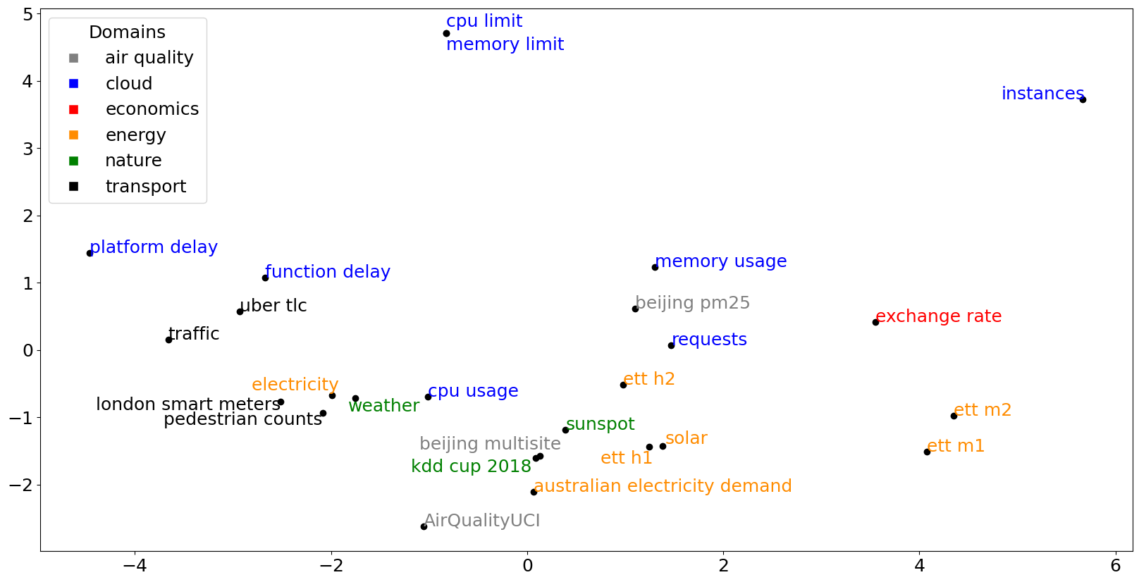
Figure 12: Principal Component Analysis (PCA) on the average catch22 features of each pre-training dataset. We take the average of the catch22 features for each dataset, standardize them, and then perform PCA on those points, such that each point corresponds to one dataset. We then visualize these points projected onto the top 2 components, and we color the name of each dataset according to its domain. The datasets are spread over both components, showing a diversity among the average catch-22 features of the different datasets. Also, datasets from different domains tend to be clustered together, which demonstrates that combining different domains increases pre-training data diversity. Together, these results suggest that combining multiple datasets across different domains increases the diversity of the pre-training data. Under the assumption that diversity in the pre-training data is beneficial for foundation model pre-training (Brown et al., 2020b), pre-training a single time series model on a diverse combination of multiple datasets from multiple domains is beneficial to the foundation model’s zero-shot and few-shot adaptation performance.

To quantify the diversity of the pretraining corpus, we analyze the properties of its datasets through 22 Canonical time series Characteristics (“catch22 features”), a set of quickly computable time series features selected for their classification ability (Lubba et al., 2019) from the features of the Highly Comparable Time Series Analysis (hctsa) library (Fulcher et al., 2013). To assess diversity across datasets, we apply PCA to the features averaged per-dataset and plot the top 2 components . We find that having multiple datasets within domains and across domains increases the diversity of AC22 features in the top 2-component space (see Figure 12 in Appendix).

7.2 Scaling Analysis

Dataset size has been shown empirically to improve performance (Kaplan et al., 2020). Constructing neural scaling laws (Kaplan et al., 2020; Caballero et al., 2023) can help understand how the performance of the model scales with respect to different parameters such as the amount of pretraining data, number of parameters in the model etc. Towards understanding these quantities for models such as Lag-Llama, we fit neural scaling laws (Caballero et al., 2023) to our model’s validation loss and present in App. § F.1 the obtained scaling laws that describe the performance of our model with respect the amount of pretraining data.

8 Discussion

We present Lag-Llama, a foundation model for univariate probabilistic time series forecasting based on a simple decoder-only transformer architecture. We show that Lag-Llama, when pretrained from scratch on a large corpus of datasets, has strong zero-shot generalization performance on unseen datasets, and performs comparably to dataset-specific models. Lag-Llama also demonstrates state-of-the-art performance across diverse datasets from different domains after finetuning, and emerges as the best general-purpose model without any knowledge of downstream datasets. Lag-Llama also demonstrates a strong few-shot adaptation performance across varying amounts of data history being available. Finally, we investigate the diversity of the pretraining corpus used to train Lag-Llama.

Our work opens up several potential directions for future work. For now, collecting and collating a large scale time series corpus of open dataset would be of high value, since the largest time series dataset repositories (Godahewa et al., 2021) are themselves too small. Further, scaling up the models further beyond the model sizes explored in this work using different training strategies constitutes an essential next step towards building even more powerful time series foundation models. Finally, expanding our work from univariate towards multivariate approaches by capturing complex multivariate dynamics of real-world datasets also constitutes an important direction for future work.

9 Impact Statement

The goal of this work is to introduce general-purpose foundation models for time series forecasting. There are many potential societal consequences of such models, including positive impacts on optimizing processes via better decision-making, as well as possible negative impacts.

To the best of our knowledge, none of the datasets used contain nor are linked to any individual or personally identifiable data, and have been sourced from referenced locations.

10 Contributions

Arjun organized, planned, and led the project overall; refined and improved the Lag-Llama architecture by refining key components (lags, sampling of the model), and refining the architecture and training strategies (such as dropout, early stopping, learning rate scheduling), iterated on the dataset choices for Lag-Llama and dataset splitting strategies, fixed issues with data window sampling, ran and iterated on all large-scale pretraining, fine-tuning and few-shot learning experiments for Lag-Llama, and wrote several main parts of the paper.

Kashif wrote the code for the Lag-Llama architecture and training strategies, conducted initial experiments for Lag-Llama and other lag-based architectures that were explored in the project; added Monash time series repository dataset to Hugging Face datasets as well as other datasets; implemented all (but one) transformer-based time series models; worked to merge fixes/features upstream to GluonTS; integrated code with Hugging Face for open-source release; and wrote several main parts of the paper.

Hena added support for time features, updated the alternative Lag-Transformer model for experiments, added support for the key-value cache for faster inference, compiled a list of all GluonTS datasets and their descriptions, and contributed to dataset compilation efforts, added utilities to track per-dataset validation and training loss, worked with the Informer, Autoformer and ETSFormer models for the paper for the large-scale experiments of the paper.

Andrew expanded the empirical design of the paper for the fine-tuning and downstream adaptation settings, ran experiments and contributed to the writing of the first version of the paper, wrote several key sections of the paper, adapted air quality and Huawei datasets, integrated robust scaler for data normalization, worked on the ideation and codebase of the Catch-22 feature-based dataset analysis for the paper.

Rishika ran experiments, and contributed to the writing of the first version of the paper, added all time series augmentations to the codebase of the paper, updated the alternative Lag-Transformer model for new experiments, adapted ETT datasets, Azure/Borg/Alibaba datasets (Cloud datasets), added options for automatic batch size search and plotting forecasts, integrated distribution heads such as IQN for experiments.

Arian ran experiments and contributed to the writing of the first version of the paper, worked with the OneFitsAll model initial code and experiments, and worked with the experiments for the N-BEATS model.

Mohammad worked with all AutoGluon models and experiments, added the option to use Stochastic Weight Averaging (SWA), and brainstormed about early stopping techniques to use when pretraining.

George ran experiments, and contributed to the writing of the first version of the paper, adapting the Electricity Household Consumption Dataset, M5, Walmart, Rossman, and Corporation and Restaurant Datasets used in the experiments of the project and the paper.

Roland worked with the code and experiments of the OneFitsAll model for all large-scale experiments in the paper, and contributed to writing several sections of the paper.

Nadhir integrated the N-BEATS model and worked with it for all large-scale experiments in the paper.

Marin wrote the initial code for sampling windows for the pretraining set and provided feedback with GluonTS code and experimental setups.

Sahil, Anderson, Nicolas, Alexandre, Valentina, and Yuriy advised the project as a whole, provided feedback on the experiments and the paper, and contributed to the writing of several sections of the paper.

Irina advised the project with feedback in several stages, contributing to the writing of the paper, acquisition of the funding for the project, and conceiving and pushing forward the research direction in the early stages of the project.

11 Acknowledgements

We are grateful to Viatcheslav Gurev, for useful discussions during the course of the project. We acknowledge and thank the authors and contributors of all the open-source libraries that were used in this work, especially: GluonTS (Alexandrov et al., 2020), NumPy (Harris et al., 2020), Pandas (Pandas development team, 2020), Matplotlib (Hunter, 2007) and PyTorch (Paszke et al., 2019).

We acknowledge the support from the Canada CIFAR AI Chair Program and from the Canada Excellence Research Chairs (CERC) Program. This project used compute resources provided by the Oak Ridge Leadership Computing Facility at the Oak Ridge National Laboratory, which is supported by the Office of Science of the U.S. Department of Energy under Contract No. DE-AC05-00OR22725. This project further used compute resources provided by ServiceNow, Mila, and Compute Canada.

Appendix A Details of Datasets

Table 3: Datasets used in the pretraining corpus and the unseen datasets on which we evaluate, grouped by the domains they are labelled against.

	Transport & Tourism	Energy	Nature	Air Quality	Cloud	Banking & Econ
Pretraining	San Francisco Traffic	Australian Electricity Demand	KDD Cup 2018	Beijing Multisite	CPU Limit Minute
	Uber TLC Hourly	Electricity Hourly	Sunspot	UCI	CPU Usage Minute
		London Smart Meters			Function Delay Minute
		Solar			Instances Minute
		Wind Farms			Memory Limit Minute
		ETT H1			Memory Usage Minute
		ETT H2
		ETT M1
Unseen	Pedestrian Counts	ETT M2	Weather	Beijing PM2.5	Requests Minute	Exchange Rate
					Platform Delay Minute

Table 4: Statistics of all the datasets used in the paper. Frequencies H stands for Hourly, T for minute, and B for business day. Tokens refers to the total number of windows of size $1$ in the dataset, computed as the aggregate number of timesteps across all series in that dataset.

Dataset	Freq	Domain	Prediction Length	Train split
				Timestamps	# Series	Tokens
Australian Electricity Demand	0.5H	Energy	60	230676	5	1153380
Electricity Hourly	H	Energy	48	26256	321	8428176
London Smart Meters	0.5H	Energy	60	23844	5560	132572640
Solar	10T	Energy	60	52500	137	7192500
Wind Farms	T	Energy	60	526980	339	178646220
Pedestrian Counts	H	Transport	48	84283	66	5562678
Uber TLC Hourly	H	Transport	24	4254	262	1114548
Traffic	H	Transport	24	14036	862	12099032
KDD Cup 2018	H	Nature	48	10850	270	2929500
Sunspot	D	Nature	30	73894	1	73894
Weather	D	Nature	30	695	3010	2091950
Exchange Rate	1B	Economic	30	6071	8	48568
ETT H1	H	Energy	24	8640	1	8640
ETT H2	H	Energy	24	8640	1	8640
ETT M1	15T	Energy	24	34560	1	34560
ETT M2	15T	Energy	24	34560	1	34560
Requests Minute	T	Cloud	60	64800	10	648000
Function Delay Minute	T	Cloud	60	64800	10	648000
Platform Delay Minute	T	Cloud	60	64800	10	648000
CPU Usage Minute	T	Cloud	60	64800	10	648000
Memory Usage Minute	T	Cloud	60	64800	10	648000
CPU Limit Minute	T	Cloud	60	64800	10	648000
Memory Limit Minute	T	Cloud	60	64800	10	648000
Instances Minute	T	Cloud	60	64800	10	648000
UCI	H	Air Quality	24	9357	13	121641
Beijing PM2.5	H	Air Quality	24	43824	8	350592
Beijing Multisite	H	Air Quality	24	35064	132	4628448

Table 5: Hyperparameter choices for Lag-Llama. The values with * represent the optimal values obtained by hyperparameter search.
^† Note that this is just the consecutive context that is sampled for each window; in practice we use a much larger context window due to the use of lags, as described in Sec. § 4.1

Hyperparameter	Lag-Llama
Number of layers	1,2,3,4,5,6,7,8*,9
Number of heads	1,2,3,4,5,6,7,8,9*
Embedding Dimensions per head	16*, 32, 64, 128, 256, 512
Context Length $C$ †	32*, 64, 128, 256, 512, 1024
Augmentation Probability	0,0.25,0.5*,1.0
Frequency Masking Rate	0,0.25,0.5*,1.0
Frequency Mixing Rate	0,0.25*,0.5,1.0
Weight Decay	0*,0.25,0.5,1.0
Dropout	0*,0.25,0.5,1.0

We use the following datasets in our experiments, the statistics of which are in Table 4, and their domains in Table 3. Table 3 further presents if a dataset was present in the pretraining or downstream testing corpora in our work.

The Air Quality UC Irvine Repository dataset (UCI) contains 9358 instances of hourly averaged responses from 5 metal oxide chemical sensors embedded in an Air Quality Chemical Multisensor Device in a polluted area (Vito, 2016).

The Australian Electricity Demand dataset comprises five half-hourly time series of the electricity demand across five Australian states: Victoria, New South Wales, Queensland, Tasmania, and South Australia (Godahewa et al., 2021).

The Beijing PM2.5 dataset contains hourly data of PM2.5 levels recorded by the US Embassy in Beijing. The dataset also includes meteorological data from Beijing Capital International Airport (Chen, 2017).

The Beijing Multi-Site Air-Quality dataset comprises hourly measurements of six primary air pollutants and six corresponding meteorological variables at various locations in Beijing over a period of four years. (Chen, 2019)

The Electricity Hourly dataset captures electricity usage for 321 clients measured at hourly intervals from 2012 to 2014 (Godahewa et al., 2021).

The ETTh1, ETTh2, ETTm1, ETTm2 datasets contain 2 years worth of data obtained from two Electricity Transformers at hourly and 15-minute frequencies curated to help predict if electrical transformers’ oil is at a safe temperature (Zhou et al., 2021b).

The Exchange Rate compilation encompasses the daily exchange rates of eight foreign currencies, namely Australia, the United Kingdom, Canada, Switzerland, China, Japan, New Zealand, and Singapore, spanning the period from 1990 to 2016 (Godahewa et al., 2021).

The Huawei cloud datasets contain serverless traces (Joosen et al., 2023). We select $8$ series containing metrics based on the minute-frequency occurrences of the top 10 functions by median occurrences over 141 days: function delay, platform delay, cpu usage, memory usage, cpu limit, memory limit, instances. platform delay, requests.

The London Smart Meters dataset focuses on electrical consumption readings from smart meters in 5,567 households that participated in the UK Power Networks Low Carbon London project between November 2011 and February 2014 (Godahewa et al., 2021).

The KDD Cup 2018 dataset comprises extensive hourly time series data reflecting air quality levels across 59 stations in Beijing and London from January 2017 to March 2018. Measurements include PM2.5, PM10, NO2, CO, O3, and SO2 (Godahewa et al., 2021).

The Pedestrian Counts dataset (referred to as ped-counts in parts of the text) encompasses hourly pedestrian counts recorded by 66 sensors within the city of Melbourne, commencing in May 2009 (Godahewa et al., 2021).

The Solar dataset comprises 6000 simulated time series for 5-minute solar power and hourly forecasts of photovoltaic power plants in the U.S. in 2006. It includes 137 time series reflecting solar power production every 10 minutes in Alabama during 2006 (Godahewa et al., 2021).

The Sunspot dataset comprises a singular extensive daily time series of sunspot numbers spanning from January 1818 to May 2020 (Godahewa et al., 2021).

The Traffic dataset encompasses 862 hourly time series depicting road occupancy rates on the freeways in the San Francisco Bay area from 2015 to 2016 (Godahewa et al., 2021).

The Uber TLC Hourly dataset consists data of 4.5 million Uber pickups in NYC (April-September 2014) and 14.3 million pickups (January-June 2015). It includes trip details for 10 other for-hire vehicle companies and aggregated data for 329 companies (FiveThirtyEight, ; Godahewa et al., 2021).

The Weather dataset includes time series of hourly climate data near Monash University, Clayton, Victoria, Australia, from January 2010 to May 2021. The data contains series for temperature, dewpoint temperature, wind speed, mean sea level pressure, relative humidity, surface solar radiation, surface thermal radiation, and total cloud cover (Godahewa et al., 2021).

The Wind Farms dataset contains minute-frequency time series data tracking the wind power production of 339 wind farms in Australia (Godahewa et al., 2021).

Appendix B Protocol Details

For all datasets used in the paper, we have a training and test split that are non-overlapping based on the timestamps, as defined in the dataset. During pretraining, for each such dataset, we exclude the $14$ last overlapping windows of the train split, and use it as the dataset’s validation set. When pretraining, we train on a combined dataset formed out of the train split of each dataset, after every epoch, we obtain the validation loss on the validation sets of all datasets used in the pretraining corpus. We use the average validation loss for early stopping criterion (this is referred to as ”validation loss” in the paper). When fine-tuning on a specific dataset, we exclude the single last window of the train split, and use it as the dataset’s validation set. We train on the train split of the dataset, and use the validation split for early stopping. We use the same setup as fine-tuning Lag-Llama, for all supervised baselines that we produce results for in the paper. Following typical evaluation setups (Shchur et al., 2023), all results reported in the paper are on the last prediction window of the test splits defined in App. § A.

Appendix C Additional Empirical Results

C.1 Results on the Pretraining Datasets

A strong foundation model should not just be good at adapting zero-shot and few-shot to unseen distributions of data, but should also perform well in-distribution, i.e. on the datasets that the model has been pretrained on. Therefore, apart from evaluating our model on unseen datasets, we also evaluate our model on those datasets we use for pretraining.

Results are given in Tab. 6, Tab. 7, and Tab. 8. Results on Average Rank on all datasets are given in Tab. 9. The training budget of Lag-Llama was split among all the pretraining datasets, while other supervised models on the dataset do not have that constraint. Thereby, Lag-Llama did not see as much data in each dataset as the other models, and thereby is not expected to perform as well as each supervised model on the specific datasets. This is reflected in the results, as Lag-Llama is not the best performing model in each dataset. Still, Lag-Llama achieves a comparable average rank, and is among the models achieving the top average ranks.

Table 6: CRPS of Lag-Llama on $7$/$20$ datasets in the pretraining corpus, compared to supervised baselines trained solely on the respective datasets. Lower is better. A mean or standard deviation of 0.0000 signifies that the first non-zero digit is beyond $3$ decimal places.

Model	Dataset
	aus-elec-demand	electricity	kdd-cup	london-smart-meters	solar	sunspot	traffic
AutoARIMA	0.065$\pm$0.000	0.098$\pm$0.003	0.552$\pm$0.000	nan$\pm$nan	0.558$\pm$0.000	77.862$\pm$0.000	0.277$\pm$0.000
AutoETS	0.160$\pm$0.000	0.104$\pm$0.000	2.350$\pm$0.000	nan$\pm$nan	0.551$\pm$0.000	171.363$\pm$0.000	0.492$\pm$0.000
CrostonSBA	0.127$\pm$0.000	0.244$\pm$0.000	0.459$\pm$0.000	0.500$\pm$0.000	1.016$\pm$0.000	34.458$\pm$0.000	0.414$\pm$0.000
DeepAR	0.043$\pm$0.000	0.085$\pm$0.005	0.327$\pm$0.014	0.409$\pm$0.000	0.446$\pm$0.002	1.390$\pm$0.000	0.100$\pm$0.000
DynamicOptimize	0.043$\pm$0.000	0.203$\pm$0.000	0.550$\pm$0.000	0.681$\pm$0.000	1.580$\pm$0.000	181.350$\pm$0.000	0.383$\pm$0.000
NPTS	0.098$\pm$0.000	0.139$\pm$0.001	0.346$\pm$0.001	0.464$\pm$0.000	0.404$\pm$0.001	201.558$\pm$10.653	0.191$\pm$0.000
PatchTST	0.056$\pm$0.000	0.088$\pm$0.001	0.432$\pm$0.043	0.375$\pm$0.000	0.734$\pm$0.002	3.083$\pm$0.000	0.153$\pm$0.001
TemporalFusionT	0.041$\pm$0.000	0.100$\pm$0.008	0.411$\pm$0.023	0.343$\pm$0.000	0.443$\pm$0.003	25.675$\pm$0.000	0.108$\pm$0.001
NBEATS	0.032$\pm$0.002	0.072$\pm$0.000	0.435$\pm$0.080	0.453$\pm$0.000	0.655$\pm$0.000	20.089$\pm$20.404	0.116$\pm$0.000
OFA	0.112$\pm$0.003	0.286$\pm$0.040	0.491$\pm$0.034	0.285$\pm$0.046	3.786$\pm$0.234	38.119$\pm$1.536	0.446$\pm$0.009
Informer	0.064$\pm$0.020	0.081$\pm$0.002	0.351$\pm$0.000	0.424$\pm$0.011	0.990$\pm$0.140	4.765$\pm$0.336	0.157$\pm$0.000
AutoFormer	0.090$\pm$0.021	0.102$\pm$0.005	0.451$\pm$0.018	0.383$\pm$0.003	2.107$\pm$0.425	40.456$\pm$12.354	0.185$\pm$0.010
ETSFormer	0.105$\pm$0.011	0.191$\pm$0.026	0.692$\pm$0.071	0.460$\pm$0.009	1.271$\pm$0.086	58.708$\pm$17.080	0.188$\pm$0.008
LagLLama	0.087$\pm$0.018	0.095$\pm$0.013	0.323$\pm$0.004	0.381$\pm$0.003	1.536$\pm$0.237	4.961$\pm$1.912	0.119$\pm$0.001

Table 7: CRPS of Lag-Llama on the $7$/$20$ datasets in the pretraining corpus, compared to supervised baselines trained solely on the respective datasets. Lower is better. A mean or standard deviation of 0.0000 signifies that the first non-zero digit is beyond $3$ decimal places.

Model	Dataset
	uber	windfarms	ETT_h1	ETT_h2	ETT_m1	AirQualityUCI	BeijingMultisite
AutoARIMA	0.322$\pm$0.000	0.084$\pm$0.000	0.120$\pm$0.000	0.095$\pm$0.000	nan$\pm$nan	0.206$\pm$0.000	0.359$\pm$0.000
AutoETS	0.461$\pm$0.000	0.096$\pm$0.000	0.117$\pm$0.000	0.105$\pm$0.000	0.073$\pm$0.000	0.220$\pm$0.000	0.472$\pm$0.000
CrostonSBA	0.427$\pm$0.000	0.130$\pm$0.000	0.123$\pm$0.000	0.112$\pm$0.000	0.094$\pm$0.000	0.237$\pm$0.000	0.400$\pm$0.000
DeepAR	0.170$\pm$0.003	0.070$\pm$0.000	0.105$\pm$0.002	0.082$\pm$0.010	0.074$\pm$0.007	0.195$\pm$0.006	0.282$\pm$0.032
DynamicOptimize	0.433$\pm$0.000	0.060$\pm$0.000	0.117$\pm$0.000	0.085$\pm$0.000	0.070$\pm$0.000	0.216$\pm$0.000	0.394$\pm$0.000
NPTS	0.191$\pm$0.000	0.208$\pm$0.000	0.268$\pm$0.001	0.216$\pm$0.001	0.162$\pm$0.000	0.130$\pm$0.001	0.414$\pm$0.006
PatchTST	0.219$\pm$0.007	0.057$\pm$0.000	0.099$\pm$0.001	0.067$\pm$0.001	0.063$\pm$0.001	0.189$\pm$0.003	0.304$\pm$0.016
TemporalFusionT	0.197$\pm$0.012	0.055$\pm$0.000	0.082$\pm$0.006	0.049$\pm$0.001	0.058$\pm$0.000	0.227$\pm$0.026	0.410$\pm$0.019
NBEATS	0.352$\pm$0.000	0.117$\pm$0.000	0.013$\pm$0.001	0.010$\pm$0.001	0.009$\pm$0.000	0.156$\pm$0.004	0.340$\pm$0.016
OFA	0.424$\pm$0.006	0.190$\pm$0.010	0.172$\pm$0.002	0.148$\pm$0.002	0.146$\pm$0.006	0.201$\pm$0.016	0.362$\pm$0.040
Informer	0.196$\pm$0.003	0.099$\pm$0.014	0.174$\pm$0.003	0.112$\pm$0.014	0.098$\pm$0.008	0.191$\pm$0.024	0.241$\pm$0.016
AutoFormer	0.205$\pm$0.007	0.246$\pm$0.038	0.155$\pm$0.010	0.119$\pm$0.005	0.119$\pm$0.008	0.172$\pm$0.012	0.238$\pm$0.012
ETSFormer	0.313$\pm$0.011	0.588$\pm$0.331	0.142$\pm$0.004	0.102$\pm$0.005	0.108$\pm$0.003	0.197$\pm$0.021	0.481$\pm$0.084
LagLLama	0.168$\pm$0.002	0.145$\pm$0.009	0.104$\pm$0.001	0.073$\pm$0.005	0.068$\pm$0.001	0.138$\pm$0.006	0.340$\pm$0.055

Table 8: CRPS of Lag-Llama on the $6$/$20$ datasets in the pretraining corpus, compared to supervised baselines trained solely on the respective datasets. Lower is better. A mean or standard deviation of 0.0000 signifies that the first non-zero digit is beyond $4$ decimal places.

Model	Dataset
	cpu_limit	cpu_usage	function_delay	instances	memory_limit	memory_usage
AutoARIMA	0.2245$\pm$0.0000	0.0814$\pm$0.0000	0.0936$\pm$0.0000	0.0121$\pm$0.0000	0.2024$\pm$0.0000	0.0326$\pm$0.0000
AutoETS	0.0632$\pm$0.0000	0.0806$\pm$0.0000	nan$\pm$nan	0.0128$\pm$0.0000	0.0632$\pm$0.0000	0.0664$\pm$0.0000
CrostonSBA	0.0278$\pm$0.0000	0.0826$\pm$0.0000	0.0756$\pm$0.0000	0.0318$\pm$0.0000	0.0278$\pm$0.0000	0.0346$\pm$0.0000
DeepAR	0.0004$\pm$0.0001	0.1034$\pm$0.0016	0.1097$\pm$0.0039	0.0179$\pm$0.0054	0.0004$\pm$0.0000	0.0147$\pm$0.0016
DynamicOptimize	0.0012$\pm$0.0000	0.0813$\pm$0.0000	0.0381$\pm$0.0000	0.0140$\pm$0.0000	0.0010$\pm$0.0000	0.0667$\pm$0.0000
NPTS	0.0001$\pm$0.0001	0.1010$\pm$0.0004	0.0808$\pm$0.0008	0.0158$\pm$0.0002	0.0001$\pm$0.0001	0.0164$\pm$0.0002
PatchTST	0.0023$\pm$0.0005	0.0805$\pm$0.0026	0.0571$\pm$0.0000	0.0104$\pm$0.0021	0.0042$\pm$0.0012	0.0172$\pm$0.0042
TemporalFusionT	0.0001$\pm$0.0001	0.0830$\pm$0.0062	0.0552$\pm$0.0030	0.0057$\pm$0.0010	0.0000$\pm$0.0000	0.0113$\pm$0.0013
NBEATS	0.0001$\pm$0.0000	0.0972$\pm$0.0018	0.0502$\pm$0.0030	0.0086$\pm$0.0012	0.0000$\pm$0.0000	0.0121$\pm$0.0009
OFA	0.0004$\pm$0.0003	0.1209$\pm$0.0082	0.1249$\pm$0.0170	0.0235$\pm$0.0019	0.0000$\pm$0.0000	0.0137$\pm$0.0012
Informer	0.0001$\pm$0.0000	0.0986$\pm$0.0040	0.0843$\pm$0.0143	0.0164$\pm$0.0000	0.0000$\pm$0.0000	0.0110$\pm$0.0004
AutoFormer	0.0392$\pm$0.0040	0.1040$\pm$0.0031	0.1652$\pm$0.0328	0.1311$\pm$0.0600	0.1489$\pm$0.0334	0.1301$\pm$0.1235
ETSFormer	0.0021$\pm$0.0015	0.1295$\pm$0.0061	0.2066$\pm$0.0774	0.5406$\pm$0.4268	1.2181$\pm$1.2744	0.0605$\pm$0.0120
LagLLama	0.0001$\pm$0.0000	0.0897$\pm$0.0013	0.0590$\pm$0.0000	0.0062$\pm$0.0010	0.0000$\pm$0.0000	0.0127$\pm$0.0007

Table 9: Average Rank Across all Pre-Training Datasets. Lower is better.

Model	Average Rank
ETSFormer	10.900
AutoETS	10.200
CrostonSBA	10.000
OFA	9.850
AutoFormer	9.550
NPTS	8.350
AutoARIMA	8.333
DynamicOptimize	8.300
Informer	6.025
DeepAR	5.125
PatchTST	4.700
LagLLama	4.625
NBEATS	4.600
TemporalFusionT	3.875

Appendix D Hyperparameters of Lag-Llama

We perform a random search of $100$ different hyperparameter configurations and use the average validation loss over all datasets in the pretraining corpus to select our model.

We list the possible hyperparameters of Lag-Llama and the optimal values obtained by our hyperparameter search in Tab. 5. Our final model obtained by hyperparameter search contains 2,449,299 parameters.

Appendix E Forecast Visualizations

We plot some sample forecasts and highlight the median, 50-th (dark green) and 90-th (light-green) prediction interval; starting from datasets in the pretraining corpus: Electricity Hourly in Figure 3, ETT-H2 in Figure 4, Traffic in Figure 5. The Zero-shot forecasts of Lag-Llama on downstream unseen datasets are highlighted for textttETT-M2 in Figure 6, Pedestrian Counts in Figure 7 and Requests Minute in Figure 8. Finally, forecasts after fine-tuning on these downstream unseen datasets are shown for ETT-M2 in Figure 9, Pedestrian Counts in Figure 10 and Requests Minute in Figure 11. Note in particular the different magnitudes of the sampled values depending on the dataset, via the same shared model.

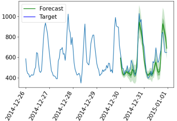
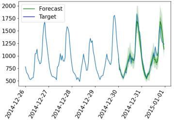
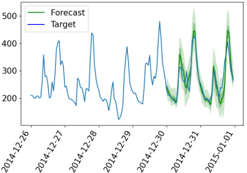
Figure 3: Forecasting examples on the Electricity Hourly dataset

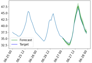
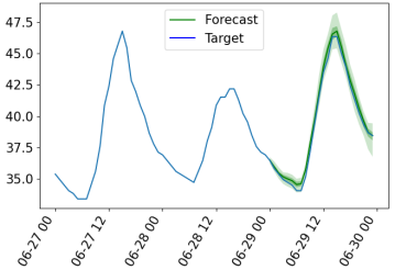
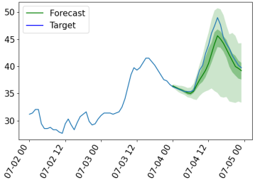
Figure 4: Forecasting examples from ETT-H2 dataset

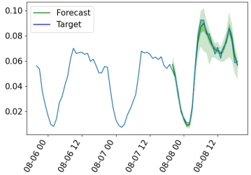
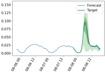
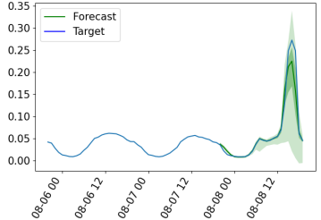
Figure 5: Forecasting examples from Traffic dataset

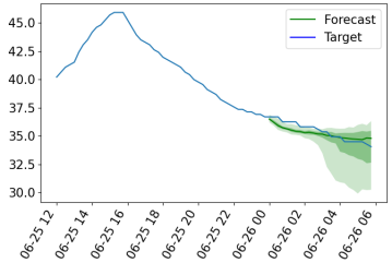
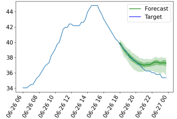
Figure 6: Zero-shot forecasting examples on the unseen downstream ETT-M2 dataset

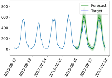
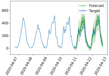
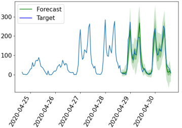
Figure 7: Zero-shot forecasting examples on the unseen downstream Pedestrian Counts dataset

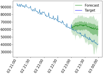
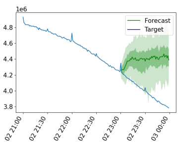
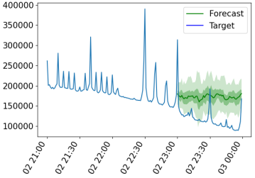
Figure 8: Zero-shot forecasting examples on the unseen downstream Requests Minute dataset

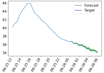
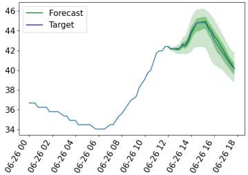
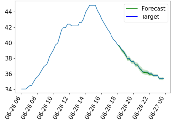
Figure 9: Lag-Llama fine-tuned forecasting examples on the downstream ETT-M2 dataset

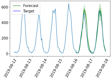
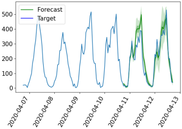
Figure 10: Lag-Llama fine-tuned forecasting examples on the downstream Pedestrian Counts dataset

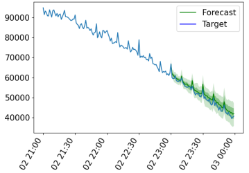
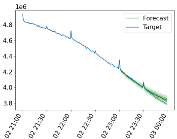
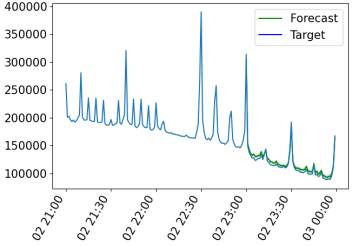
Figure 11: Lag-Llama fine-tuned forecasting examples on the downstream Requests Minute dataset

Appendix F Additional Visualizations

F.1 Neural Scaling Laws

The parameters of the Neural Scaling Law (Caballero et al., 2023) fit in Figure 13 to the validation loss ($y)$ with respect to the pretraining data epochs seen ($x$) (where each epoch is $100$ randomly sampled windows) are given below.

$$y =a+\left(bx^{-c_{0}}\right)\prod_{i=1}^{n}\left(1+\left(\frac{x}{d_{i}}\right)^{1/f_{i}}\right)^{-c_{i}*f_{i}}$$

$$a =-6.1167$$

$$b =8.01589$$

$$c_{0} =0.0155$$

$$c_{1} =-0.1043$$

$$d_{1} =1.6423e-36$$

$$f_{1} =-36.4660$$

With such a law, one can extrapolate the validation loss of the model and predict performance in larger dataset regimes (Figure 13). As efforts progress towards collating better data repositories for time series foundation model training, such laws can help quantify the relations between the data used and the performance of the model.

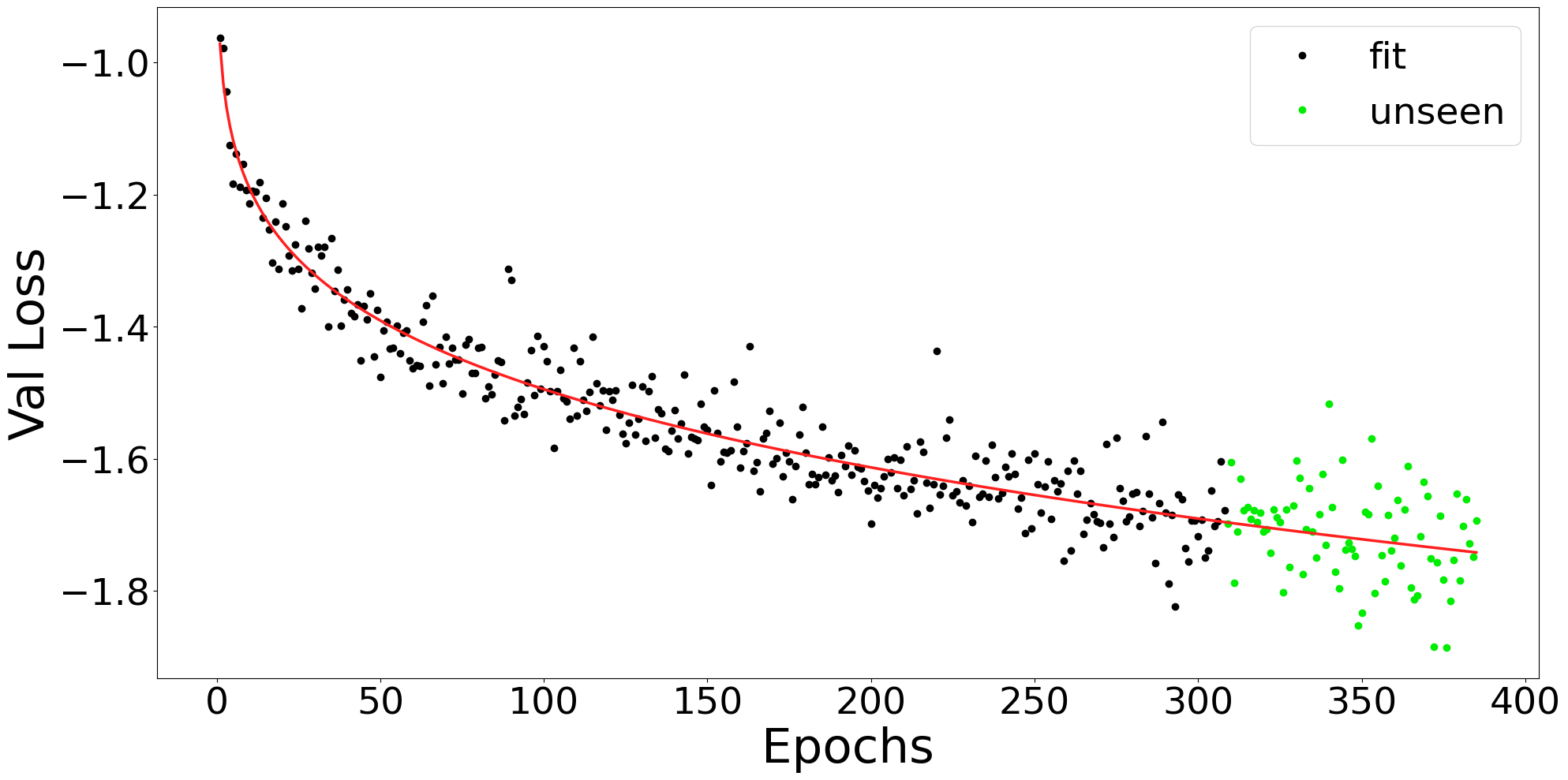
Figure 13: A neural scaling law fit to the validation loss (negative log-likelihood) of our foundation model, averaged across 3 seeds. ”fit” represents points from the validation curve used for constructing the scaling law. ”unseen” represents points of the validation curve that are predicted with the constructed scaling. We use a 60/20/20 train/val/test split to fit our scaling law.

References

- Alexandrov et al. (2020) Alexandrov, A., Benidis, K., Bohlke-Schneider, M., Flunkert, V., Gasthaus, J., Januschowski, T., Maddix, D. C., Rangapuram, S., Salinas, D., Schulz, J., Stella, L., Türkmen, A. C., and Wang, Y. GluonTS: Probabilistic and Neural Time Series Modeling in Python. Journal of Machine Learning Research, 21(116):1–6, 2020. URL http://jmlr.org/papers/v21/19-820.html.
- Anonymous (2024) Anonymous. TEMPO: Prompt-based generative pre-trained transformer for time series forecasting. In The Twelfth International Conference on Learning Representations, 2024. URL https://openreview.net/forum?id=YH5w12OUuU.
- Ashok et al. (2023) Ashok, A., Étienne Marcotte, Zantedeschi, V., Chapados, N., and Drouin, A. Tactis-2: Better, faster, simpler attentional copulas for multivariate time series, 2023.
- Assimakopoulos & Nikolopoulos (2000) Assimakopoulos, V. and Nikolopoulos, K. The theta model: a decomposition approach to forecasting. International Journal of Forecasting, 16(4):521–530, 2000. ISSN 0169-2070. doi: https://doi.org/10.1016/S0169-2070(00)00066-2. URL https://www.sciencedirect.com/science/article/pii/S0169207000000662. The M3- Competition.
- Benidis et al. (2022) Benidis, K., Rangapuram, S. S., Flunkert, V., Wang, Y., Maddix, D., Turkmen, C., Gasthaus, J., Bohlke-Schneider, M., Salinas, D., Stella, L., Aubet, F.-X., Callot, L., and Januschowski, T. Deep learning for time series forecasting: Tutorial and literature survey. ACM Computing Surveys, 55(6):1–36, 12 2022. doi: 10.1145/3533382. URL https://doi.org/10.1145%2F3533382.
- Bommasani et al. (2022) Bommasani, R., Hudson, D. A., Adeli, E., Altman, R., Arora, S., von Arx, S., Bernstein, M. S., Bohg, J., Bosselut, A., Brunskill, E., Brynjolfsson, E., Buch, S., Card, D., Castellon, R., Chatterji, N., Chen, A., Creel, K., Davis, J. Q., Demszky, D., Donahue, C., Doumbouya, M., Durmus, E., Ermon, S., Etchemendy, J., Ethayarajh, K., Fei-Fei, L., Finn, C., Gale, T., Gillespie, L., Goel, K., Goodman, N., Grossman, S., Guha, N., Hashimoto, T., Henderson, P., Hewitt, J., Ho, D. E., Hong, J., Hsu, K., Huang, J., Icard, T., Jain, S., Jurafsky, D., Kalluri, P., Karamcheti, S., Keeling, G., Khani, F., Khattab, O., Koh, P. W., Krass, M., Krishna, R., Kuditipudi, R., Kumar, A., Ladhak, F., Lee, M., Lee, T., Leskovec, J., Levent, I., Li, X. L., Li, X., Ma, T., Malik, A., Manning, C. D., Mirchandani, S., Mitchell, E., Munyikwa, Z., Nair, S., Narayan, A., Narayanan, D., Newman, B., Nie, A., Niebles, J. C., Nilforoshan, H., Nyarko, J., Ogut, G., Orr, L., Papadimitriou, I., Park, J. S., Piech, C., Portelance, E., Potts, C., Raghunathan, A., Reich, R., Ren, H., Rong, F., Roohani, Y., Ruiz, C., Ryan, J., Ré, C., Sadigh, D., Sagawa, S., Santhanam, K., Shih, A., Srinivasan, K., Tamkin, A., Taori, R., Thomas, A. W., Tramèr, F., Wang, R. E., Wang, W., Wu, B., Wu, J., Wu, Y., Xie, S. M., Yasunaga, M., You, J., Zaharia, M., Zhang, M., Zhang, T., Zhang, X., Zhang, Y., Zheng, L., Zhou, K., and Liang, P. On the opportunities and risks of foundation models, 2022.
- Box & Jenkins (1976) Box, G. and Jenkins, G. Time Series Analysis: Forecasting and Control. Holden-Day series in time series analysis and digital processing. Holden-Day, 1976. ISBN 9780816211043. URL https://books.google.ca/books?id=1WVHAAAAMAAJ.
- Brown et al. (2020a) Brown, T., Mann, B., Ryder, N., Subbiah, M., Kaplan, J. D., Dhariwal, P., Neelakantan, A., Shyam, P., Sastry, G., Askell, A., Agarwal, S., Herbert-Voss, A., Krueger, G., Henighan, T., Child, R., Ramesh, A., Ziegler, D., Wu, J., Winter, C., Hesse, C., Chen, M., Sigler, E., Litwin, M., Gray, S., Chess, B., Clark, J., Berner, C., McCandlish, S., Radford, A., Sutskever, I., and Amodei, D. Language models are few-shot learners. In Larochelle, H., Ranzato, M., Hadsell, R., Balcan, M. F., and Lin, H. (eds.), Advances in Neural Information Processing Systems, volume 33, pp. 1877–1901. Curran Associates, Inc., 2020a. URL https://proceedings.neurips.cc/paper/2020/file/1457c0d6bfcb4967418bfb8ac142f64a-Paper.pdf.
- Brown et al. (2020b) Brown, T., Mann, B., Ryder, N., Subbiah, M., Kaplan, J. D., Dhariwal, P., Neelakantan, A., Shyam, P., Sastry, G., Askell, A., et al. Language models are few-shot learners. Advances in neural information processing systems, 33:1877–1901, 2020b.
- Caballero et al. (2023) Caballero, E., Gupta, K., Rish, I., and Krueger, D. Broken neural scaling laws. In The Eleventh International Conference on Learning Representations, 2023. URL https://arxiv.org/abs/2210.14891.
- Chan et al. (2022) Chan, S., Santoro, A., Lampinen, A., Wang, J., Singh, A., Richemond, P., McClelland, J., and Hill, F. Data distributional properties drive emergent in-context learning in transformers. Advances in Neural Information Processing Systems, 35:18878–18891, 2022.
- Chang et al. (2023) Chang, C., Peng, W.-C., and Chen, T.-F. Llm4ts: Two-stage fine-tuning for time-series forecasting with pre-trained llms, 2023.
- Chen et al. (2023) Chen, M., Xu, Z., Zeng, A., and Xu, Q. Fraug: Frequency domain augmentation for time series forecasting, 2023. URL https://openreview.net/forum?id=j83rZLZgYBv.
- Chen (2017) Chen, S. Beijing PM2.5 Data. UCI Machine Learning Repository, 2017. DOI: https://doi.org/10.24432/C5JS49.
- Chen (2019) Chen, S. Beijing Multi-Site Air-Quality Data. UCI Machine Learning Repository, 2019. DOI: https://doi.org/10.24432/C5RK5G.
- Chowdhery et al. (2022) Chowdhery, A., Narang, S., Devlin, J., Bosma, M., Mishra, G., Roberts, A., Barham, P., Chung, H. W., Sutton, C., Gehrmann, S., Schuh, P., Shi, K., Tsvyashchenko, S., Maynez, J., Rao, A., Barnes, P., Tay, Y., Shazeer, N., Prabhakaran, V., Reif, E., Du, N., Hutchinson, B., Pope, R., Bradbury, J., Austin, J., Isard, M., Gur-Ari, G., Yin, P., Duke, T., Levskaya, A., Ghemawat, S., Dev, S., Michalewski, H., Garcia, X., Misra, V., Robinson, K., Fedus, L., Zhou, D., Ippolito, D., Luan, D., Lim, H., Zoph, B., Spiridonov, A., Sepassi, R., Dohan, D., Agrawal, S., Omernick, M., Dai, A. M., Pillai, T. S., Pellat, M., Lewkowycz, A., Moreira, E., Child, R., Polozov, O., Lee, K., Zhou, Z., Wang, X., Saeta, B., Diaz, M., Firat, O., Catasta, M., Wei, J., Meier-Hellstern, K., Eck, D., Dean, J., Petrov, S., and Fiedel, N. Palm: Scaling language modeling with pathways, 2022.
- Croston (1972) Croston, J. D. Forecasting and stock control for intermittent demands. Operational Research Quarterly (1970-1977), 23(3):289–303, 1972. ISSN 00303623. URL http://www.jstor.org/stable/3007885.
- Dekking et al. (2005) Dekking, F. M., Kraaikamp, C., Lopuhaä, H. P., and Meester, L. E. A Modern Introduction to Probability and Statistics: Understanding why and how, volume 488. Springer, 2005.
- Devlin et al. (2019) Devlin, J., Chang, M.-W., Lee, K., and Toutanova, K. BERT: Pre-training of deep bidirectional transformers for language understanding. In Proceedings of the 2019 Conference of the North American Chapter of the Association for Computational Linguistics: Human Language Technologies, Volume 1 (Long and Short Papers), pp. 4171–4186, Minneapolis, Minnesota, June 2019. Association for Computational Linguistics. doi: 10.18653/v1/N19-1423. URL https://aclanthology.org/N19-1423.
- Drouin et al. (2022) Drouin, A., Marcotte, E., and Chapados, N. TACTiS: Transformer-attentional copulas for time series. In Chaudhuri, K., Jegelka, S., Song, L., Szepesvari, C., Niu, G., and Sabato, S. (eds.), Proceedings of the 39th International Conference on Machine Learning, volume 162 of Proceedings of Machine Learning Research, pp. 5447–5493. PMLR, 07 2022. URL https://proceedings.mlr.press/v162/drouin22a.html.
- Fatemi et al. (2023) Fatemi, Z., Huynh, M.-T. T., Zheleva, E., Syed, Z., and Di, X. Mitigating cold-start forecasting using cold causal demand forecasting model. ArXiv, abs/2306.09261, 2023. URL https://api.semanticscholar.org/CorpusID:259164537.
- (22) FiveThirtyEight. Uber tlc foil response. https://github.com/fivethirtyeight/uber-tlc-foil-response.
- Fulcher et al. (2013) Fulcher, B. D., Little, M. A., and Jones, N. S. Highly comparative time-series analysis: the empirical structure of time series and their methods. Journal of the Royal Society Interface, 10(83):20130048, 2013.
- Gneiting & Raftery (2007) Gneiting, T. and Raftery, A. E. Strictly proper scoring rules, prediction, and estimation. Journal of the American Statistical Association, 102(477):359–378, 2007. doi: 10.1198/016214506000001437. URL https://doi.org/10.1198/016214506000001437.
- Godahewa et al. (2021) Godahewa, R., Bergmeir, C., Webb, G. I., Hyndman, R. J., and Montero-Manso, P. Monash time series forecasting archive. In Neural Information Processing Systems Track on Datasets and Benchmarks, 2021.
- Gulati et al. (2020) Gulati, A., Qin, J., Chiu, C.-C., Parmar, N., Zhang, Y., Yu, J., Han, W., Wang, S., Zhang, Z., Wu, Y., and Pang, R. Conformer: Convolution-augmented transformer for speech recognition, 2020.
- Harris et al. (2020) Harris, C. R., Millman, K. J., van der Walt, S. J., Gommers, R., Virtanen, P., Cournapeau, D., Wieser, E., Taylor, J., Berg, S., Smith, N. J., Kern, R., Picus, M., Hoyer, S., van Kerkwijk, M. H., Brett, M., Haldane, A., del R’ıo, J. F., Wiebe, M., Peterson, P., G’erard-Marchant, P., Sheppard, K., Reddy, T., Weckesser, W., Abbasi, H., Gohlke, C., and Oliphant, T. E. Array programming with NumPy. Nature, 585(7825):357–362, September 2020. doi: 10.1038/s41586-020-2649-2. URL https://doi.org/10.1038/s41586-020-2649-2.
- Hunter (2007) Hunter, J. D. Matplotlib: A 2D graphics environment. Computing in Science & Engineering, 9(3):90–95, 2007. doi: 10.1109/MCSE.2007.55.
- Hyndman & Athanasopoulos (2018) Hyndman, R. and Athanasopoulos, G. Forecasting: Principles and Practice. OTexts, Australia, 2nd edition, 2018.
- Hyndman & Athanasopoulos (2021) Hyndman, R. and Athanasopoulos, G. Forecasting: Principles and practice. OTexts, 2021. ISBN 978-0987507136.
- Hyndman & Khandakar (2008) Hyndman, R. J. and Khandakar, Y. Automatic time series forecasting: The forecast package for R. J. Stat. Soft., 27(3):1–22, 2008. ISSN 1548-7660. doi: 10.18637/jss.v027.i03. URL https://doi.org/10.18637/jss.v027.i03.
- Jin et al. (2023) Jin, M., Wang, S., Ma, L., Chu, Z., Zhang, J. Y., Shi, X., Chen, P.-Y., Liang, Y., Li, Y.-F., Pan, S., and Wen, Q. Time-llm: Time series forecasting by reprogramming large language models, 2023.
- Joosen et al. (2023) Joosen, A., Hassan, A., Asenov, M., Singh, R., Darlow, L., Wang, J., and Barker, A. How does it function? characterizing long-term trends in production serverless workloads. In Proceedings of the 2023 ACM Symposium on Cloud Computing, SoCC ’23, pp. 443–458, New York, NY, USA, 2023. Association for Computing Machinery. ISBN 9798400703874. doi: 10.1145/3620678.3624783. URL https://doi.org/10.1145/3620678.3624783.
- Kaplan et al. (2020) Kaplan, J., McCandlish, S., Henighan, T., Brown, T. B., Chess, B., Child, R., Gray, S., Radford, A., Wu, J., and Amodei, D. Scaling laws for neural language models. arXiv preprint arXiv:2001.08361, 2020.
- Li et al. (2019) Li, S., Jin, X., Xuan, Y., Zhou, X., Chen, W., Wang, Y.-X., and Yan, X. Enhancing the locality and breaking the memory bottleneck of transformer on time series forecasting. In Wallach, H., Larochelle, H., Beygelzimer, A., d'Alché-Buc, F., Fox, E., and Garnett, R. (eds.), Advances in Neural Information Processing Systems, volume 32. Curran Associates, Inc., 2019. URL https://proceedings.neurips.cc/paper_files/paper/2019/file/6775a0635c302542da2c32aa19d86be0-Paper.pdf.
- Li et al. (2023) Li, Z., Wang, P., Rao, Z., Pan, L., and Xu, Z. Ti-MAE: Self-supervised masked time series autoencoders, 2023. URL https://openreview.net/forum?id=9AuIMiZhkL2.
- Lim et al. (2021) Lim, B., Arık, S. O., Loeff, N., and Pfister, T. Temporal fusion transformers for interpretable multi-horizon time series forecasting. International Journal of Forecasting, 37(4):1748–1764, 2021. ISSN 0169-2070. doi: https://doi.org/10.1016/j.ijforecast.2021.03.012. URL https://www.sciencedirect.com/science/article/pii/S0169207021000637.
- Liu et al. (2022a) Liu, S., Yu, H., Liao, C., Li, J., Lin, W., Liu, A. X., and Dustdar, S. Pyraformer: Low-complexity pyramidal attention for long-range time series modeling and forecasting. In International Conference on Learning Representations, 2022a. URL https://openreview.net/forum?id=0EXmFzUn5I.
- Liu et al. (2023) Liu, X., Hu, J., Li, Y., Diao, S., Liang, Y., Hooi, B., and Zimmermann, R. Unitime: A language-empowered unified model for cross-domain time series forecasting, 2023.
- Liu et al. (2022b) Liu, Y., Wu, H., Wang, J., and Long, M. Non-stationary transformers: Exploring the stationarity in time series forecasting. In Oh, A. H., Agarwal, A., Belgrave, D., and Cho, K. (eds.), Advances in Neural Information Processing Systems, 2022b. URL https://openreview.net/forum?id=ucNDIDRNjjv.
- Lubba et al. (2019) Lubba, C. H., Sethi, S. S., Knaute, P., Schultz, S. R., Fulcher, B. D., and Jones, N. S. catch22: Canonical time-series characteristics: Selected through highly comparative time-series analysis. Data Mining and Knowledge Discovery, 33(6):1821–1852, 2019.
- Matheson & Winkler (1976) Matheson, J. E. and Winkler, R. L. Scoring Rules for Continuous Probability Distributions. Management Science, 22(10):1087–1096, 1976.
- Ni et al. (2023) Ni, Z., Yu, H., Liu, S., Li, J., and Lin, W. Basisformer: Attention-based time series forecasting with learnable and interpretable basis. In Thirty-seventh Conference on Neural Information Processing Systems, 2023. URL https://openreview.net/forum?id=xx3qRKvG0T.
- Nie et al. (2023a) Nie, Y., H. Nguyen, N., Sinthong, P., and Kalagnanam, J. A time series is worth 64 words: Long-term forecasting with transformers. In International Conference on Learning Representations, 2023a.
- Nie et al. (2023b) Nie, Y., Nguyen, N. H., Sinthong, P., and Kalagnanam, J. A time series is worth 64 words: Long-term forecasting with transformers. In The Eleventh International Conference on Learning Representations, 2023b. URL https://openreview.net/forum?id=Jbdc0vTOcol.
- OpenAI (2023) OpenAI. Gpt-4 technical report, 2023.
- Oreshkin et al. (2020a) Oreshkin, B. N., Carpov, D., Chapados, N., and Bengio, Y. N-beats: Neural basis expansion analysis for interpretable time series forecasting. In International Conference on Learning Representations, 2020a. URL https://openreview.net/forum?id=r1ecqn4YwB.
- Oreshkin et al. (2020b) Oreshkin, B. N., Carpov, D., Chapados, N., and Bengio, Y. N-BEATS: Neural basis expansion analysis for interpretable time series forecasting. In International Conference on Learning Representations, 2020b. URL https://openreview.net/forum?id=r1ecqn4YwB.
- Pandas development team (2020) Pandas development team, T. pandas-dev/pandas: Pandas, February 2020. URL https://doi.org/10.5281/zenodo.3509134.
- Paszke et al. (2019) Paszke, A., Gross, S., Massa, F., Lerer, A., Bradbury, J., Chanan, G., Killeen, T., Lin, Z., Gimelshein, N., Antiga, L., Desmaison, A., Kopf, A., Yang, E., DeVito, Z., Raison, M., Tejani, A., Chilamkurthy, S., Steiner, B., Fang, L., Bai, J., and Chintala, S. PyTorch: An imperative style, high-performance deep learning library. In Wallach, H., Larochelle, H., Beygelzimer, A., d’Alché Buc, F., Fox, E., and Garnett, R. (eds.), Advances in Neural Information Processing Systems 32, pp. 8026–8037. Curran Associates, Inc., 2019.
- Peterson (2017) Peterson, M. An Introduction to Decision Theory. Cambridge Introductions to Philosophy. Cambridge University Press, second edition, 2017. doi: 10.1017/9781316585061.
- Radford et al. (2019) Radford, A., Wu, J., Child, R., Luan, D., Amodei, D., and Sutskever, I. Language models are unsupervised multitask learners. 2019.
- Radford et al. (2021) Radford, A., Kim, J. W., Hallacy, C., Ramesh, A., Goh, G., Agarwal, S., Sastry, G., Askell, A., Mishkin, P., Clark, J., Krueger, G., and Sutskever, I. Learning transferable visual models from natural language supervision, 2021.
- Rasul et al. (2021a) Rasul, K., Seward, C., Schuster, I., and Vollgraf, R. Autoregressive denoising diffusion models for multivariate probabilistic time series forecasting. In Meila, M. and Zhang, T. (eds.), Proceedings of the 38th International Conference on Machine Learning, volume 139 of Proceedings of Machine Learning Research, pp. 8857–8868. PMLR, 18–24 Jul 2021a. URL https://proceedings.mlr.press/v139/rasul21a.html.
- Rasul et al. (2021b) Rasul, K., Sheikh, A.-S., Schuster, I., Bergmann, U. M., and Vollgraf, R. Multivariate probabilistic time series forecasting via conditioned normalizing flows. In International Conference on Learning Representations, 2021b. URL https://openreview.net/forum?id=WiGQBFuVRv.
- Robert Verkuil (2022) Robert Verkuil, Ori Kabeli, Y. D. e. a. Language models generalize beyond natural proteins, 2022.
- Salinas et al. (2019a) Salinas, D., Bohlke-Schneider, M., Callot, L., Medico, R., and Gasthaus, J. High-dimensional multivariate forecasting with low-rank Gaussian copula processes. In Advances in Neural Information Processing Systems, volume 32, pp. 6827–6837, 2019a.
- Salinas et al. (2019b) Salinas, D., Flunkert, V., Gasthaus, J., and Januschowski, T. DeepAR: Probabilistic forecasting with autoregressive recurrent networks. International Journal of Forecasting, 2019b. ISSN 0169-2070. URL http://www.sciencedirect.com/science/article/pii/S0169207019301888.
- Salinas et al. (2020) Salinas, D., Flunkert, V., Gasthaus, J., and Januschowski, T. DeepAR: Probabilistic forecasting with autoregressive recurrent networks. International Journal of Forecasting, 36(3):1181–1191, 2020.
- Shchur et al. (2023) Shchur, O., Turkmen, A. C., Erickson, N., Shen, H., Shirkov, A., Hu, T., and Wang, B. Autogluon–timeseries: AutoML for probabilistic time series forecasting. In AutoML Conference 2023 (ABCD Track), 2023. URL https://openreview.net/forum?id=XHIY3cQ8Tew.
- Student (1908) Student. The probable error of a mean. Biometrika, pp. 1–25, 1908.
- Su et al. (2021) Su, J., Lu, Y., Pan, S., Wen, B., and Liu, Y. Roformer: Enhanced transformer with rotary position embedding, 2021.
- Syntetos & Boylan (2005) Syntetos, A. A. and Boylan, J. E. The accuracy of intermittent demand estimates. International Journal of Forecasting, 21(2):303–314, 2005. ISSN 0169-2070. doi: https://doi.org/10.1016/j.ijforecast.2004.10.001. URL https://www.sciencedirect.com/science/article/pii/S0169207004000792.
- Tay et al. (2022) Tay, Y., Dehghani, M., Abnar, S., Chung, H. W., Fedus, W., Rao, J., Narang, S., Tran, V. Q., Yogatama, D., and Metzler, D. Scaling laws vs model architectures: How does inductive bias influence scaling?, 2022.
- Thrun & Pratt (1998) Thrun, S. and Pratt, L. Learning to Learn: Introduction and Overview, pp. 3–17. Kluwer Academic Publishers, USA, 1998. ISBN 0792380479.
- Torres et al. (2021) Torres, J. F., Hadjout, D., Sebaa, A., Martínez-Álvarez, F., and Troncoso, A. Deep learning for time series forecasting: a survey. Big Data, 9(1):3–21, 2021.
- Touvron et al. (2023) Touvron, H., Lavril, T., Izacard, G., Martinet, X., Lachaux, M.-A., Lacroix, T., Rozière, B., Goyal, N., Hambro, E., Azhar, F., Rodriguez, A., Joulin, A., Grave, E., and Lample, G. Llama: Open and efficient foundation language models. arXiv preprint arXiv:2302.13971, 2023.
- Vaswani et al. (2017) Vaswani, A., Shazeer, N., Parmar, N., Uszkoreit, J., Jones, L., Gomez, A. N., Kaiser, L., and Polosukhin, I. Attention is all you need. In Guyon, I., Luxburg, U. V., Bengio, S., Wallach, H., Fergus, R., Vishwanathan, S., and Garnett, R. (eds.), Advances in Neural Information Processing Systems, volume 30. Curran Associates, Inc., 2017. URL https://proceedings.neurips.cc/paper/2017/file/3f5ee243547dee91fbd053c1c4a845aa-Paper.pdf.
- Vito (2016) Vito, S. Air Quality. UCI Machine Learning Repository, 2016. DOI: https://doi.org/10.24432/C59K5F.
- Wang et al. (2022) Wang, W., Bao, H., Dong, L., Bjorck, J., Peng, Z., Liu, Q., Aggarwal, K., Mohammed, O. K., Singhal, S., Som, S., and Wei, F. Image as a foreign language: Beit pretraining for all vision and vision-language tasks, 2022.
- Wen et al. (2018) Wen, R., Torkkola, K., Narayanaswamy, B., and Madeka, D. A multi-horizon quantile recurrent forecaster, 2018.
- Wikipedia (2024) Wikipedia. Cold start (recommender systems) — Wikipedia, the free encyclopedia. http://en.wikipedia.org/w/index.php?title=Cold%20start%20(recommender%20systems)&oldid=1172519745, 2024. [Online; accessed 01-February-2024].
- Woo et al. (2022a) Woo, G., Liu, C., Sahoo, D., Kumar, A., and Hoi, S. CoST: Contrastive learning of disentangled seasonal-trend representations for time series forecasting. In International Conference on Learning Representations, 2022a. URL https://openreview.net/forum?id=PilZY3omXV2.
- Woo et al. (2022b) Woo, G., Liu, C., Sahoo, D., Kumar, A., and Hoi, S. Etsformer: Exponential smoothing transformers for time-series forecasting, 2022b.
- Woo et al. (2023) Woo, G., Liu, C., Sahoo, D., Kumar, A., and Hoi, S. ETSformer: Exponential smoothing transformers for time-series forecasting, 2023. URL https://openreview.net/forum?id=5m_3whfo483.
- Wu et al. (2021) Wu, H., Xu, J., Wang, J., and Long, M. Autoformer: Decomposition transformers with auto-correlation for long-term series forecasting. In Beygelzimer, A., Dauphin, Y., Liang, P., and Vaughan, J. W. (eds.), Advances in Neural Information Processing Systems, 2021. URL https://openreview.net/forum?id=J4gRj6d5Qm.
- Wu et al. (2022) Wu, H., Xu, J., Wang, J., and Long, M. Autoformer: Decomposition transformers with auto-correlation for long-term series forecasting, 2022.
- Wu et al. (2020a) Wu, N., Green, B., Ben, X., and O’Banion, S. Deep transformer models for time series forecasting: The influenza prevalence case, 2020a.
- Wu et al. (2020b) Wu, S., Xiao, X., Ding, Q., Zhao, P., Wei, Y., and Huang, J. Adversarial sparse transformer for time series forecasting. In Larochelle, H., Ranzato, M., Hadsell, R., Balcan, M., and Lin, H. (eds.), Advances in Neural Information Processing Systems, volume 33, pp. 17105–17115. Curran Associates, Inc., 2020b. URL https://proceedings.neurips.cc/paper_files/paper/2020/file/c6b8c8d762da15fa8dbbdfb6baf9e260-Paper.pdf.
- Yeh et al. (2023) Yeh, C.-C. M., Dai, X., Chen, H., Zheng, Y., Fan, Y., Der, A., Lai, V., Zhuang, Z., Wang, J., Wang, L., and Zhang, W. Toward a foundation model for time series data, 2023.
- Zhang & Sennrich (2019) Zhang, B. and Sennrich, R. Root mean square layer normalization. In Wallach, H., Larochelle, H., Beygelzimer, A., d'Alché-Buc, F., Fox, E., and Garnett, R. (eds.), Advances in Neural Information Processing Systems, volume 32. Curran Associates, Inc., 2019. URL https://proceedings.neurips.cc/paper_files/paper/2019/file/1e8a19426224ca89e83cef47f1e7f53b-Paper.pdf.
- Zhou et al. (2021a) Zhou, H., Zhang, S., Peng, J., Zhang, S., Li, J., Xiong, H., and Zhang, W. Informer: Beyond efficient transformer for long sequence time-series forecasting. Proceedings of the AAAI Conference on Artificial Intelligence, 35(12):11106–11115, May 2021a. URL https://ojs.aaai.org/index.php/AAAI/article/view/17325.
- Zhou et al. (2021b) Zhou, H., Zhang, S., Peng, J., Zhang, S., Li, J., Xiong, H., and Zhang, W. Informer: Beyond efficient transformer for long sequence time-series forecasting. In The Thirty-Fifth AAAI Conference on Artificial Intelligence, AAAI 2021, Virtual Conference, volume 35, pp. 11106–11115. AAAI Press, 2021b.
- Zhou et al. (2021c) Zhou, H., Zhang, S., Peng, J., Zhang, S., Li, J., Xiong, H., and Zhang, W. Informer: Beyond efficient transformer for long sequence time-series forecasting, 2021c.
- Zhou et al. (2022) Zhou, T., Ma, Z., Wen, Q., Wang, X., Sun, L., and Jin, R. FEDformer: Frequency enhanced decomposed transformer for long-term series forecasting. In Chaudhuri, K., Jegelka, S., Song, L., Szepesvari, C., Niu, G., and Sabato, S. (eds.), Proceedings of the 39th International Conference on Machine Learning, volume 162 of Proceedings of Machine Learning Research, pp. 27268–27286. PMLR, 17–23 Jul 2022. URL https://proceedings.mlr.press/v162/zhou22g.html.
- Zhou et al. (2023a) Zhou, T., Niu, P., Wang, X., Sun, L., and Jin, R. One fits all:power general time series analysis by pretrained lm, 2023a.
- Zhou et al. (2023b) Zhou, T., Niu, P., Wang, X., Sun, L., and Jin, R. One fits all: Power general time series analysis by pretrained LM. In Thirty-seventh Conference on Neural Information Processing Systems, 2023b. URL https://openreview.net/forum?id=gMS6FVZvmF.