Five years of 6.7 GHz methanol maser monitoring with Irbene radio telescopes

Abstract

We present the results of a 5-year monitoring program of 42 sources targeted at 6.7 GHz methanol masers, conducted from March 2017 to October 2022 using the Irbene 32 and 16 meter radio telescopes. Sources were observed with irregular intervals where time between two consecutive observation ranged from twenty four hours to thirty five days. We found that more than 55 per cent of the sources showed significant variability, but often only one or a few spectral features were varying significantly. Numerous type of variability were found in our sample: low-variable, periodic, irregular, synchronised and anti-correlated between features and steadily raising or falling flux. Our analysis techniques also uncover new variability trends for several sources. The maser monitoring program is one of the first single-dish science initiatives at the Irbene radio telescope complex, initiated shortly after the instrument’s reconstruction and upgrades. Our findings unequivocally demonstrate its suitability for maser research purposes.

1 Introduction

The formation of high-mass stars is still a challenging topic in modern astrophysics with a key question being, how a massive star attains its ultimate mass. Two prevailing theories that tackle this issue are ‘global collapse’ and ‘competitive accretion’ (e.g. Zinnecker & Yorke 2007, for review). Studying high-mass star-forming regions (HMSFRs) through observations poses significant challenges due to their typically large distances, obscuration caused by interstellar dust, and rapid evolution. Recently, 6.7 GHz methanol masers have emerged as a unique and valuable tool for studying HMSFRs, as they serve as prominent signposts of the radiative conditions these regions (e.g., Menten 1991). The spectral features of these masers are remarkably bright and narrow. Methanol maser emission has been suggested to appear during the early stages of protostellar evolution (Walsh et al., 1998). Most of the observed 6.7 GHz methanol masers are associated with protostellar discs (van der Walt et al., 2007), although several cases where the masers trace outflows has also been reported (Goddi et al., 2011).

Early insights into 6.7 GHz methanol maser variability were gleaned from surveys focused on discovering new masers. A notable study by Caswell et al. (1995) involved observing a sample of 245 sources 4 to 5 times over a 1.5-year period. The results indicated that only 48 sources from the 245 sample showed significant variability, and often only one or several spectral components in these variable sources exhibited high variability. Two epoch (separated by 2 years) multi-beam survey found that 5 to 7 per cent of a 972 source sample showed flux density changes by a factor of two or more (Breen et al., 2015).

The two largest long term methanol maser monitoring surveys according to our knowledge ware conducted by Goedhart et al. (2004) and Szymczak et al. (2018). Goedhart et al. (2004) reported 6.7 GHz maser flux density changes of 54 sources over a duration of 4.2 years, monitoring with 2 – 4 observations per month, transitioning to daily observation for rapidly variable sources. Szymczak et al. (2018) conducted a 3.7–year monitoring campaign of 166 sources with 2 – 4 observations per week. Goedhart et al. (2004) classified spectral features as variable if the derived variability index (see section 2.4, equation (1)) was higher than 0.5. Szymczak et al. (2018) used a different approach based on the variability properties on individual spectral features (see section 2.4 of their paper). Nevertheless, Szymczak et al. (2018) found that fractions of low-variable (and non-variable) sources in both samples are very similar – 19 and 21 percent accordingly. Furthermore they (Goedhart et al. 2004 and Szymczak et al. 2018) concluded that there are two different kinds of the 6.7 GHz methanol maser line variability: flaring (which refers to fastest flux increases in a short time, e.g. flux increase by factor of two in two weeks) and gradual (including periodic) changes of flux densities.

We would like to highlight the Ibaraki 6.7 GHz Methanol Maser Monitoring (iMet) program by Yonekura et al. (2016). The Japanese team conducts regular monitoring of 442 sources, making it the largest sample for a monitoring campaign by far. Furthermore, they consistently publish their 6.7 GHz methanol maser flux measurements in an open-access database. To our knowledge, only a summary of periodic methanol maser variability has been published (Sugiyama et al., 2019a).

The discovery of periodic variability came as an unexpected finding, with known periods ranging from 24 to 600 days, observed in some or all features. Furthermore, researchers have noticed phase-lags between individual maser lines (Goedhart et al. 2004; Goedhart et al. 2014; Fujisawa et al. 2014a and Szymczak et al. 2016). The majority of theoretical models addressing periodic masers involve a binary nature of the central object, where the observed changes in maser flux density are modulated by periodic variations of pumping radiation, in response to orbital movements (Araya et al. 2010; van der Walt 2011; and Parfenov & Sobolev 2014). However, as one exception, Inayoshi et al. (2013) proposed a model suggesting periodic pulsations of young stars due to mass growth during rapid accretion periods.

Maser flares display significantly more rapid variability, with flux increasing several times over a short period. It is worth noting that there is no agreed-upon threshold of variability to define as flare among radio astronomers. Among the most remarkable and extensively studied flares are the methanol maser outbursts caused by accretion bursts in sources like S255IR$-$NIRS3 and G358.93$-$0.03 (Caratti o Garatti et al. 2017; Stecklum et al. 2021). Monitoring efforts by single-dish radiotelescopes has proven to be an effective tool for identifying these extraordinary events (Fujisawa et al. 2015; Szymczak et al. 2018; MacLeod et al. 2018 and Burns et al. 2020).

The causes of variability in 6.7 GHz methanol masers continue to be a prominent area of research. Caswell et al. (1995) proposed that maser variations are a result of changes in the gain path length caused by large-scale gas motions. In periodic 6.7 GHz sources, a strong correlation between maser and infrared flux densities has been observed (e.g., Olech et al. 2020, 2022; Kobak et al. 2023), indicating that the pumping rate plays a dominant role. A series of studies that combine single-dish time series with high angular resolution Very Large Baseline interferometry (VLBI) data have shown that most of the 6.7 GHz methanol maser variability is caused by variations in pumping rates (e.g., Szymczak et al. 2014; Moscadelli et al. (2017); Olech et al. 2019 and Durjasz et al. 2019).

In this paper, we present the results of a flux density monitoring for 42 methanol maser sources, spanning up to 5 years. This program’s initial goals and source list was firstly presented in Aberfelds et al. (2017). Our main motivation was to investigate maser variability and assess the capabilities of the Irbene facility for maser observations and highlighting the importance of maser monitoring. Previously mentioned extraordinary methanol maser outburst (S255IR$-$NIRS3 and G358.93$-$0.03 Fujisawa et al. 2015; Sugiyama et al. 2019b) have been detected by medium-size radiotelescopes, very similar to those in Irbene. The Irbene facility has a rich and unusual history. After the downfall of the Soviet Union, these military severance antennas were left in poor technical condition for two decades. However, between 2014 and 2016, the radiotelescopes underwent reconstruction, upgrades, and were equipped to modern standards, making scientific studies finally feasible with this instrument. As a relatively recent asset to the broader radio-astronomy community, several scientific programs have been realised. Including studies of Solar Corona activities, Active Galactic Nuclei (AGN) monitoring, the maser monitoring program presented in this study, monitoring of fast radio bursts (FRBs) under the framework of PRECISE project, and participation in the European VLBI Network (EVN) (Sukharev et al. 2022, Younes et al. 2022, and Ryabov & Vrublevskis 2023 as examples). Parts of monitoring results for separate methanol maser sources are reported in Salii et al. (2022); Aberfelds et al. (2021) and Aberfelds et al. (2023). This is the first proper reporting of a complete set of our 6.7 GHz methanol maser monitoring results.

2 Observations

2.1 Instrumentation and methods

The 32 m and 16 m radio telescopes (RT–32 and RT–16, respectively) operated by Ventspils International Radio Astronomy Center (VIRAC), located in Irbene, Latvia were used for the monitoring of the 6668.519 MHz methanol maser transition. The flux density was sampled with irregular frequency, but typically, each source in our 42 source sample was observed once every 5 to 7 days. Sources exhibiting noticeably faster variability (e.g., more than a 33 percent flux difference for a spectral component between two observations) were selected for daily observations in order to delineate periods of enhanced activity. There are several up to thirty–day gaps in moitoring observations due to scheduling constraints and a few instances when both telescopes were not operational. Around 95 per cent of measurements were carried out on the RT–16.

Both telescopes are equipped with broad band 4.5 – 8.8 GHz dual–polarisation receivers. The signal chains for both telescopes are identical. The wide-band feed-horns are optimised for each telescope’s geometry, and both are calibrated and operated in the same manner. The RT–32 has a half-power beam-width (HPBW) of 6 arcmin but it suffers from relatively strong side lobes which may cause confusion, the HPBW of the RT–16 is 12 arcmin. The best practically achievable pointing accuracy is 30 arcsec for both telescopes. Estimated telescope efficiencies are  0.4 and  0.8 for RT-32 and RT–16, respectively. Surface accuracy (rms) of RT–32 primary mirror is around 3.2 mm and 635 $\mu$m for RT–16. Both telescopes use a noise diode with generated signal of (T_cal) of 3.82 K. Elevation depended Degrees Per Flux Units (DPFU) at zenith are 0.086 K Jy^-1 and 0.046 K Jy^-1, for RT–32 and RT–16, respectively (Bleiders et al., 2017). Both telescopes use fast Fourier transform (FFT) back-end spectrometers based on the Ettus Research USRP X300 software-defined radio (SDR) platform (Bleiders et al., 2020). Standard setup parameters for monitoring observations were 4096 channels per 1.5625 MHz band giving 0.017 km s^-1 spectral resolution. Frequency switching mode (Winkel et al., 2012) was used with four 15 sec long integration stages (first pair with noise diode off, last pair with noise diode on). Typical on–source integration times were 15 min averaging multiple foursome stages together. Stages that produced unsatisfactory results can be omitted from the averaging if needed.

Systems were regularly calibrated using stable continuum sources obtained from Perley & Butler (2013) and by stable maser sources like G32.744–0.076; G69.540-0.976 and G75.782+0.34 (Szymczak et al., 2018). For adequate pointing accuracy, we employed antenna Field System (FS) (Himwich, 2000) pointing models, which are regularly calibrated by observing strong continuum sources. Under good observation conditions, the system temperatures were 28 K and 33 K for the RT–32 and RT–16, respectively. Data processing was done using an in–house developed software package maser-data-processing-suite (mdps) described in detail by Steinbergs et al. (2021).

2.2 Source selection

Sources were selected from the Torun methanol source catalogue (Szymczak et al., 2012) with the following criteria: declination above -10^∘ and peak flux density above 3 Jy. A significant portion of our selected sources have been extensively studied in the past, enabling comparison of our results with those of previous research. Several sources were added later, as follow up observations in reaction to alerts of heightened maser activity from the Maser Monitoring Organization. The complete list of targets is given in Table 1. The source names are given according to their Galactic coordinates, their coordinates and systemic radial velocities (V_lsr) are obtained from Szymczak et al. (2012) with the exception of G85.411+0.002 for which observation parameters were provided by private communication with the Maser Monitoring Organization.

Table 1: Methanol maser sources monitored at 6.7 GHz, under our monitoring program.

Source	RA(J2000)	Dec(J2000)	Vlsr
	(h m s)	(o ’ ")	(km s-1)
G22.357+0.066	18 31 44.12	-09 22 12.3	79.4
G24.33+0.14	18 35 08.09	-07 35 03.6	112.0
G25.709+0.044	18 38 03.15	-06 24 14.9	95.5
G25.64+1.05	18 34 21.99	-05 59 38.6	41.0
G30.99-0.08	18 48 10.80	-01 45 39.3	77.8
G32.04+0.06	18 49 36.6	-00 45 45.6	92.7
G32.744-0.076	18 51 21.87	-00 12 05.3	35.0
G33.641-0.228	18 53 32.56	00 31 39.2	60.0
G35.20-1.74	19 01 46.90	01 13 07.5	44.0
G34.396+0.222	18 53 18.00	01 25 24.55	60.0
G36.705+0.096	18 57 59.123	03 24 06.11	62.2
G37.479-0.105	19 00 07.14	03 59 53.3	59.1
G37.43+01.51	18 54 14.23	04 41 41.1	41.3
G37.55+0.20	18 59 09.986	04 12 15.6	85.0
G43.149+0.013	19 10 11.05	09 05 20.4	15.0
G43.796-0.12	19 11 54.016	09 35 49.46	40.0
G45.071+0.132	19 13 22.129	10 50 53.11	57.8
G49.04-1.08	19 25 22.30	13 47 20.1	37.1
G196.454-01.677	06 14 37.03	13 49 36.6	14.7
G49.490-0.388	19 23 43.96	14 30 35.0	57.9
G192.60-0.05	06 12 54.02	17 59 23.3	6.5
G189.030+0.784	06 08 40.67	21 31 06.9	9.6
G59.783+0.065	19 43 11.25	23 44 03.3	19.5
G69.540-0.976	20 10 09.074	31 31 35.95	7.5
G174.20-0.08	05 30 48.01	33 47 54.6	3.5
G173.482+2.446	05 39 13.06	35 45 51.3	-12.0
G73.06+1.80	20 08 10.20	35 59 23.7	6.1
G75.782+0.34	20 21 44.20	37 26 36.7	-0.5
G78.122+3.633	20 14 25.88	41 13 36.87	-6.5
G81.88+0.78	20 38 36.45	42 37 36.1	5.5
G188.95+0.89	06 08 53.34	42 37 36.1	10.5
G85.411+0.002	20 54 13.689	44 54 07.686	-29.4
G90.92+1.49	21 09 12.60	50 01 02.9	-69.2
G94.602$-$1.796	21 39 58.26	50 14 20.9	-43.0
G123.066-6.309	00 52 24.20	56 33 43.2	-31.0
G111.26-0.77	23 16 10.00	59 55 31.3	-37.0
G111.542+0.777	23 13 45.36	61 28 10.6	-56.2
G133.947+1.064	02 27 03.82	61 52 25.4	-43.0
G109.871+2.114	22 56 17.90	62 01 49.7	-3.5
G121.298+0.659	00 36 47.35	63 29 02.2	-25.8
G107.298+5.639	22 21 26.81	63 51 37.14	-8.5
G108.184+5.519	22 28 51.41	64 13 41.3	-11.0

2.3 Error evaluation

As mentioned above, both instruments were calibrated and operated identically. Long-term pointing precision control suggest an average target offset of 2 arcmin for RT–16 and 1.1 arcmin for RT–32 corresponding to 92 per cent of normalized power. System temperature stability estimations suggest this contributes as a relatively minor (no more than 5 per cent) cause of amplitude error (Antyufeyev et al., 2020). Individual measurement error was estimated as two times the noise signal standard deviation $\sigma$ (with average values of 1.9 and 0.9 Jy for RT–16 and RT–32, respectively) plus signal amplitude $A$ multiplied by relative error $\eta$ (ranging from 7 to 22 per cent) i.e. $2\sigma+A\eta$. Relative error was estimated from the comparison of multiple intrinsically low-variable source flux measurements with their corresponding mean flux densities. Observational data with clearly excessive noise levels, abnormally high system temperature or spectra with bad baseband slopes were discarded to maintain the integrity of the final averaged results. Overall, we conclude that absolute amplitude uncertainty is around 20 per cent. To avoid falsely interpreting instrumental effects as source variability, we took several actions: observations were scheduled at as consistent as possible elevation angles for a given source, avoiding observations during strong winds and rain, and by conducting regular calibration sessions.

2.4 Variability parameters

From the obtained source spectra, the tracked flux densities of the components (as shown in light curves and used for variability analysis) are measured at their corresponding peak channels. In other words, each spectral line has a specific radial velocity, and we report the flux from the channel with the highest intensity. Doppler correction for local standard of rest frame was used to align measurements at different epochs. Since methanol as a paramagnetic molecule shows a only weak polarisation distribution (Gray, 2012), to increase the signal-to-noise (S/N) ratio for further analysis we used a flux value averaged over both polarisations.

To characterise variability of a spectral feature, the same statistical tools e.g. variability index, were employed, as done by Szymczak et al. (2018) and Goedhart et al. (2004). The variability index, originally introduced by Stetson (1996), but reintroduced in a more usable form by Aller et al. (2003) is:

$$VI=\frac{(S_{max}-\sigma_{max})-(S_{min}+\sigma_{min})}{(S_{max}-\sigma_{max})+(S_{min}+\sigma_{min})}$$ (1)

Here, $S_{max}$ and $S_{min}$ are highest and lowest flux density values, respectively, and $\sigma_{max}$ and $\sigma_{min}$ are absolute flux uncertainties in these measurements. $VI$ values range from 0 for non–variable behaviour to 1 for strongly variable lines. Occasionally value can be negative, indicating that measurement uncertainty is larger than the measurement value itself. It should be noted that $VI$ is also significantly affected by outliers, as, in essence, only two measurement values are used.

Introduced by Aller et al. (2003), the fluctuation index, in our opinion, provides a better statistical tool to characterise low signal-to-noise spectral features and low-amplitude variability. It also has the advantage of a lower sensitivity to outliers. Fluctuation index measures spread versus the mean flux density value.

$$FI=\left[\frac{N}{\sum_{i=1}^{N}\sigma_{i}^{2}}\left(\frac{\sum_{i=1}^{N}S_{i}^{2}\sigma_{i}^{2}-\overline{S}\sum_{i=1}^{N}S_{i}\sigma_{i}^{2}}{N-1}-1\right)\right]^{0.5}/\overline{S}$$ (2)

Here, $S_{i}$ is an individual flux density measured in specific epoch $i$, $\overline{S}$ is the average flux density over the time interval under evaluation, $\sigma_{i}$ is the individual measurement uncertainty and $N$ is the number of measurements.

Following Szymczak et al. (2018), we also included the $\chi^{2}_{r}$ parameter as our final metric for evaluating variability:

$$\chi^{2}_{r}=\frac{1}{N-1}\sum_{i=1}^{N}\left(\frac{S_{i}-\overline{S}}{\sigma_{i}}\right)^{2}$$ (3)

For intrinsically non-variable sources this parameter will be close to unity.

2.5 Wavelet analyses

Wavelet spectral analysis has emerged as a new and powerful tool for studying monitoring data. We used open source script pycwt (Sebastian et al., 2023) which follows the approach suggested by Torrence & Compo (1998) and Liu et al. (2007) for time series analyses. Time series input, script parameters and visualisation suggestions are made following pycwt documentation and examples there. Wavelet transformation requires input data to be sampled at regular intervals which is not typically the case for maser monitoring observations, thus data re-sampling is necessary. For this purpose a linear interpolation function interp1d from scipy (Virtanen et al., 2020) was used. These re-sampled data sets were normalised by standard deviation and de-trended by linear a function. Global Wavelet Spectra in combination with Fast Fourier Transformation (FFT) using re-sampled and de-trended data, and Lomb-Scargle periodogram (Scargle, 1982) using the original data set, were used to search for periodicity signals in the maser time series.

Wavelet analysis plots (e.g. Figure 2.) show: panel a), obtained light curve denoted with red dots, overlaid with linearly interpolated time series, shown as a black line. Panel b) shows the Wavelet Power spectrum of time series in which the x and y axes represent time and period, and colour indicates the strength or power of the signal’s frequency components at that particular time and frequency (Torrence & Compo, 1998). More intense colours indicate higher power or stronger presence of periodicity at a particular frequency. The crossed out area represents combinations of time and signal periods which are affected by boundary effects i.e. the cone of influence. Panel c) shows the global wavelet power spectrum, which represents the overall presence of a particular frequency in the entire time span, overlaid with the FFT spectra and Lomb-Scargle periodogram. Here also a 95 per cent confidence level for significant frequency components in the time series are presented. Note that the y axes of b) and c) panels have logarithmic scale and trivial relations between frequency and period are used. We consider a source to have a statistically significant period in their time series if global wavelet power spectra, FFT and Lomb-Scargle periodogram display agreement and show a clear signal over 95 per cent confidence.

3 Results

We have conducted extensive flux monitoring for forty-two 6.7 GHz methanol masers, spanning up to five years. During the observing program, we noticed various maser variability types. The summary of source variability by types, described below, are presented in Table 2.

Low–variable. We categorise a maser source as having low variability when the variability indexes for all its spectral components are below 0.25. In this category are 21 per cent sources from our sample. Note, G133.947+1.064/W3(OH) two low-intensity lines at -41.8 and -42.2 km s^-1, which, due to significant blending, are excluded from our analyses, despite their variability.

Moderately variable. The variability index of the most variable component falls between 0.26 and 0.5. This variability type constitutes 26 percent of all sources.

Highly variable. A source is classified as highly variable if the variability index of at least one of its spectral components is above 0.5. This criterion was met for 55 percent of the sources in our study.

Correlated fluctuations. In this category, sources with two or more spectral features whose variability time series show a high (>0.7) positive correlation coefficient. Only sources with notable variability (variability index >0.25) are considered, we found that 19 per cent of sources have this variability type.

Anti–correlated fluctuations. Similar to the above but for spectral features exhibiting high (<-0.7) negative correlation coefficient. For example: in G33.641-0.228 the feature pair at 59.6 and 59.3 km s^-1 are anti-correlated with features at 63.2 and 62.7 km s^-1; in G109.871+2.114/Cepheus A, the feature at -2.1 km s^-1 is strongly anti - correlated with features at -3.7, -4.0 and -4.7 km s^-1. Only 7 per cent of our sources have this type of variability.

Velocity drifting. Refers to a continuous change in the radial velocity of a spectral line, with a drift of at least several spectral channels (>0.07 km s^-1) of the observed maximum velocity of the line. In our sample, only a single source (G121.298+0.659 see Figure 8.), or 2 percent, exhibited this kind of behaviour.

Cyclical variability. This category comprises sources with statistically probable periodical variability. In this work we used wavelet analyses and the Lomb-Scargle periodogram to identify statistical probable (wavelet spectrum, FFT and Lomb-Scargle all agrees and show clear signal over 95 percent confidence, see section 2.5) periodic signals. In this category are 19 per cent of sources from our sample. Parameters of sources with this variability type are summarised in Table 3. We show: the approximate period of variability, observed amount of flux change cycles, flux variation range (typical minimum and maximum flux levels for the spectral line), percentage of relative flux increase from the minimum and we provide a bibliographic references for previously identified periodicity in known sources.

Raising. A source is considered to be rising if its flux density steadily increases by more than 50 percent over a period of 100 days. We observed this rising flux trend in 7 percent of the sources in our sample.

Falling. Similarly, if a spectral feature steadily loses flux by more than 50 percent in less than 100 days, we classify it as a falling flux source. We observed this type of flux decrease in 10 percent of sources. Importantly, there is a significant overlap between the rising and falling flux sources, where the flux density of the same spectral components alternately and steadily increases or decreases.

Flaring. As mentioned before a flare is a rapid increase in maser flux density. We propose identifying a flux increase as a flare when the flux density exceeds above a rolling mean flux and five times the statistical standard deviation of the flux within that time span. More details on our flare definition are given in Section 4. If the period of increased flux extends beyond 25 days, we further classify it as a long flare. Conversely, if the flux returns to its usual levels in less than 25 days, we categorize it as a short flare. After a flare, we see that the flux usually returns to its pre-flare intensity, but the rise and decline profiles of flare are often source-distinctive, as noted by Szymczak et al. (2018). We detected flaring activity in 10 percent of the sources in our sample.

The mean values of variability parameters in our sample are 0.33 for the variability index, 0.54 for the fluctuation index and 4.66 for the $\chi^{2}_{r}$ parameter. The highest variability index in our sample was found to be 0.99 for the periodically flaring G107.298+5.63. This maser source also has the highest fluctuation index and $\chi^{2}_{r}$ parameter ($FI$ = 6.76 and $\chi^{2}_{r}$ = 307.6). Overall, all spectral components of G107.298+5.639 have highly variable parameters, indicating that it is the most variable source in our sample. Most of the identified variable lines with a variability index above 0.5 are found in low flux (S_P $\leqslant$ 30 Jy) maser features. Similar relations were found with the fluctuation index and $\chi^{2}_{r}$ parameter, which aligns with the findings of Goedhart et al. (2004) and Szymczak et al. (2018). There is a clear positive correlation trend between the variability index, fluctuation index, and the $\chi^{2}_{r}$ parameter. In total, we found 54 out of 190 spectral features to be highly variable ($VI$ > 0.5), belonging to 24 different sources, with 15 of them being faint features.

Table 2: Detected variability types

Source	Variability type
G22.357+0.066	Highly variable; Correlated fluctuations; Cyclical
G24.33+0.14	Highly variable; Long flare
G25.709+0.044	Low–variable
G25.64+1.05	Moderately variable
G30.99-0.08	Highly variable
G32.04+0.06	Moderately variable; Cyclical
G32.744-0.076	Low–variable
G33.641-0.228	Highly variable; Correlated fluctuations; Long flare
	Anti–correlated fluctuations; Short flare; Cyclical
G35.20-1.74	Highly variable; Correlated fluctuations; Falling
G34.396+0.222	Moderately variable
G36.705+0.096	Low–variable
G37.479-0.105	Low–variable
G37.43+01.51	Low–variable
G37.55+0.20	Moderately variable; Correlated fluctuations; Cyclical
G43.149+0.013	Low–variable
G43.796-0.12	Low–variable; Correlated fluctuations
G45.071+0.132	Low–variable
G49.04-1.08	Highly variable
G196.454-01.677	Highly variable; Correlated fluctuations; Cyclical
G49.490-0.388	Moderately variable
G192.60-0.05	Highly variable; Cyclical
G189.030+0.784	Highly variable
G59.783+0.065	Highly variable; Raising; Falling;
	Anti–correlated fluctuations
G69.540-0.976	Moderately variable
G174.20-0.08	Highly variable; Falling
G173.482+2.446	Moderately variable
G73.06+1.80	Highly variable; Cyclical
G75.782+0.34	Highly variable
G78.122+3.633	Highly variable; Falling;
	Raising; Correlated fluctuations
G81.88+0.78	Moderately variable
G188.95+0.89	Highly variable
G85.411+0.002	Moderately variable; Long flare
G90.92+1.49	Moderately variable
G94.602$-$1.796	Highly variable
G123.066-6.309	Highly variable
G111.26-0.77	Highly variable
G111.542+0.777	Moderately variable
G133.947+1.064	Low–variable
G109.871+2.114	Highly variable; Correlated fluctuations;
	Anti–correlated fluctuations
G121.298+0.659	Highly variable; Raising; Falling; Velocity drifting
G107.298+5.639	Highly variable; Short flare; Cyclical
G108.184+5.519	Highly variable

Table 3: Parameters of periodic (cyclical) sources. The variation range displays the typical minimum and maximum flux densities within a cycle. In the case of several spectral lines following the same periodic pattern, we utilized the parameters of the most intense lines. The relative increase indicates the percentage by which the minimum amplitude increased during the cycle.

Source	Approximate Period	Observed number of	Variation	Relative	Reference
	days	cycles	range (Jy)	Increase (%)
G22.357+0.066	170	9.2	11-37	240	Szymczak et al. (2011)
G32.04+0.06	57	11	108-200	90	This work
G33.641-0.228	500	4.4	5-55	100	Olech et al. (2019)
G33.641-0.228	115	7	40-95	130	This work
G37.55+0.20	250	5.2	3-13	330	Araya et al. (2010)
G73.06+1.80	123	5	4-14	250	Szymczak et al. (2015)
G192.60-0.05	235	5.5	60-120	100	This work
G196.454-01.67	110	7	5-32	600	Szymczak et al. (2018)
G107.298+5.63	34.4	43	*-250	$>2.5\times 10^{4}$	Szymczak et al. (2016)
* Flux regularly fell bellow our detection level.

Time series for selected sources whose high variability and interesting trends merit additional discussion are presented in Figure 1. Variability parameters for these three sources are summarised in Table 4, and for all monitored sources in our sample in Table B. Variability analyses for G78.122$+$3.633, G90.925$+$1.486 and G94.602$-$1.796 are presented in Aberfelds et al. (2023).

Table 4: Statistics of the maser line variability time-series. Here, V_P(km s^-1) is a spectral feature’s velocity at LSR, S_P(Jy) is mean flux density value for given spectral component, $VI$ and $FI$ – variability and fluctuation indexes and $\chi^{2}_{r}$ parameter. MJD_s is the start time of observations in Modified Julian Date, $T\textsubscript{s}$ is the total time-span of observation in years, $N$ - number of observations.

VP(km s-1)	SP(Jy)	$VI$	$FI$	$\chi^{2}_{r}$
G107.298+5.639 (MJDs=58298, $T\textsubscript{s}$= 4.285 y, $N$=1823)
-16.7	1.71	0.91	3.09	1.96
-11.0	1.53	0.61	0.81	1.10
-9.2	7.46	0.98	6.76	23.56
-8.6	4.30	0.88	1.76	8.21
-7.4	27.04	0.99	4.81	307.60
G33.641-0.228 (MJDs=57821, $T\textsubscript{s}$= 5.707 y, $N$=1136)
59.3	18.78	0.83	1.05	17.86
59.6	15.40	0.73	0.77	2.18
60.3	161.73	0.21	0.50	2.66
61.0	49.98	0.49	0.65	4.56
62.7	18.39	0.32	0.18	0.56
63.2	15.21	0.39	0.16	0.28
G192.60-0.05 (MJDs=57856, $T\textsubscript{s}$= 5.476 y, $N$=368)
2.3	7.47	0.92	2.52	8.66
4.2	7.19	0.67	0.78	1.68
4.8	15.75	0.63	0.74	2.52
5.9	176.91	0.37	0.52	3.07
6.3	161.27	0.81	1.59	17.11
7.5	4.48	0.97	4.24	6.27

Variability parameters for all sources are presented in Table B.

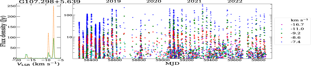
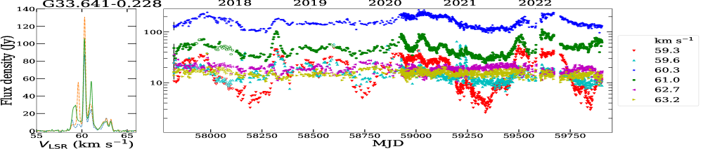
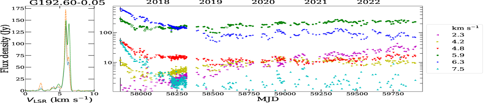
Figure 1: Spectra and light curves of the 6.7 GHz maser emission in the selected objects. Left-hand panels: maximum (orange), minimum (blue) and some average (green) spectra that, we think, best represents usual flux densities. Right-hand panels: light curves of main features. The filled and empty symbols represent the data from the 16-m and 32-m telescopes, respectively. Typical measurement uncertainty is shown by the bar for the first data point, calculated as stated in section 2.3. Note logarithmic scale.

3.1 G107.298+5.639

G107.298+5.639 is a very variable source with periodical flares, between which maser emission is under our detection level (Figure 1. top). In total, we have observed 43 flares of all spectral features during the 4.3 years, and according to their expected period of 34.4 days (Szymczak et al., 2016), only 2 flares are missing in our time series due to gaps. The rate of observations was increased from once a week to several observations per hour. The overall observed variability is consistent with the results of Szymczak et al. (2016). The spectral feature at -7.4 km s^-1 is always the most intense, and its peak intensity may vary up to a factor of ten from flare to flare. There are noticeable time lags, for example the spectral feature at -8.6 km s^-1 peaks around 2.2 days before the -7.4 and -9.2 km s^-1 features (see Figure 3.) and these delays between components’ peak flux moments are consistent flare to flare. Wavelet analyses of the -7.4 km s^-1 spectral feature’s time series are presented in Figure 2. Where panel a) shows original data (red dots) overlaid with re-sampled, de-trended and normalised time series (black line). Panel b) shows a Morlet Wavelet power spectrum and panel c) shows the Global Wavelet powers spectrum overlaid with the FFT spectrum and Lomb-Scargle periodogram. Figure 2 clearly shows a significant 35 day periodic signal, which is consistent with the results of Szymczak et al. (2016). Overall the wavelet analyses method produces expected results.

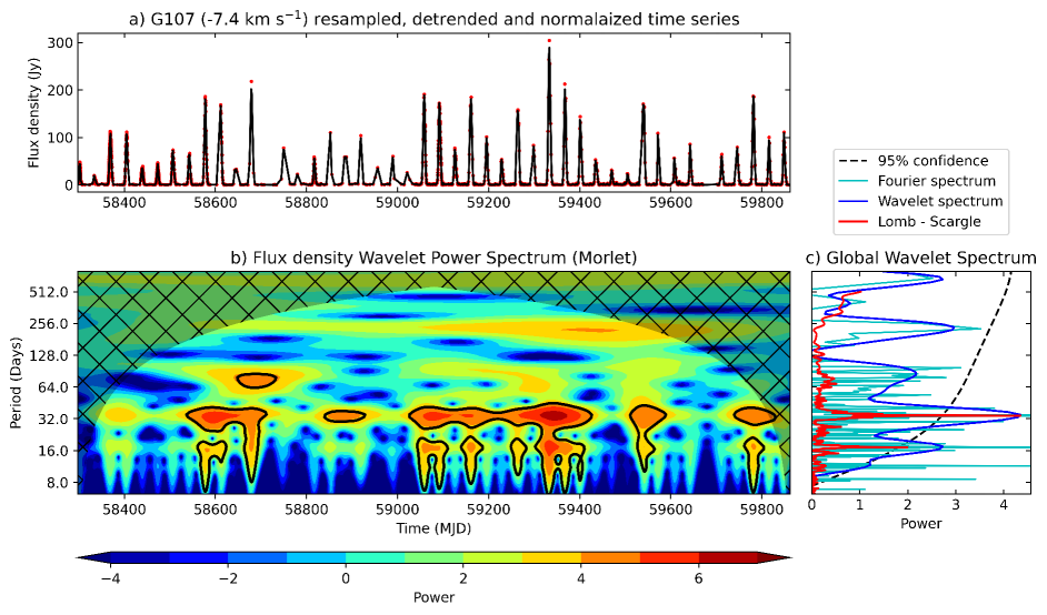
Figure 2: a) Original G107.298+5.639 -7.4 km s^-1 data denoted with red dots overlaid with regularly re-sampled, de-trended and normalised time series black line. b) Morlet wavelet power spectrum. c) Global wavelet power spectrum with significance level, additionally Fourier spectrum and Lomb - Scargle periodigram is also shown.

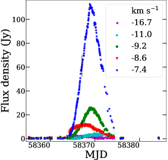
Figure 3: Example of one G107.298+5.639 flare, demonstrating time lags between spectral components, a result made possible by the high–cadence observations. During the flare, flux density was sampled every 15 minutes.

3.2 G33.641-0.22

At the beginning, our target was to observe G33.641-0.22 once per every 4 days but, starting from 58929 MJD (March 2020), we switched to daily observations in response to it’s high variability. Features at 59.3 and 59.6 km s^-1 are strongly correlated and simultaneously anti-correlated with features at 62.7 and 63.2 km s^-1. During the observation campaign we detected several flicker-like bursts similar to those previously reported by Fujisawa et al. (2014b). According to our observations, new flares happened at 58153, 58167, 58601, 58895, 59015, 59103, 59170, 59216, 59241, 59264 MJD. Two additional bursts of feature at 61.0 km s^-1 were detected, from 58270 to 58371 (Jun to September 2018) and 59460 to 59550 MJD (September to December 2021). Figure 4 highlights the regularities found in the time series. There is a strong indication of long-duration period of 500 days which is in agreement with the findings of Olech et al. (2019). Additionally, there is a tentative detection of a shorter, approximately 115-day, periodic fluctuation, which coexists with other variability patterns. Note that these shorter period fluctuations are noticeable (have high power spectra) only in three periods: from 58150 to 58550 MJD (February 2018 to March 2019); from 58815 to 59180 MJD (full year from Decembers 2019 to 2020) and from 59350 to 59750 MJD (May 2021 to Jun 2022), coinciding with high flux density phases of this component (see Figure 4.).

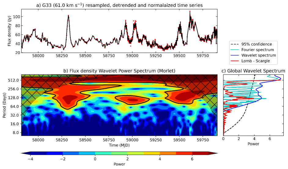
Figure 4: Same as Figure 2., but for the G33.641-0.22 61.0 km s^-1 line.

3.3 G192.60-0.05

G192.60-0.05 is also know as S255IR. This source was extensively studied during its massive flare event (Fujisawa et al. 2015 and Moscadelli et al. 2017). Our methanol maser monitoring program started monitoring in February 2017 when the S255IR maser flare was already in its declining stage. Spectral features with high flux density (5.9 and 6.3 km s^-1) continued to dim until 58325 MJD (July 2018), by a factor of 6, before becoming mostly stable, around 58600 MJD (April 2019). Starting from around 58600 MJD, the 6.3 km s^-1 line may exhibit semi–regular fluctuations (Figure 5.). Notably, the wavelet power spectra indicates periodic fluctuations with increasing duration which may explain why Lomb - Scargle and other the methods do not agree well for the most probable length of periodicity (170 and 235 days respectively). Other spectral components do not show such fluctuations. The spectral line at 7.6 km s^-1 faded down to our measurement noise level at around 58200 MJD (March 2018). Around 58000 MJD (September 2017), a new spectral feature at 2.3 km s^-1 appeared.

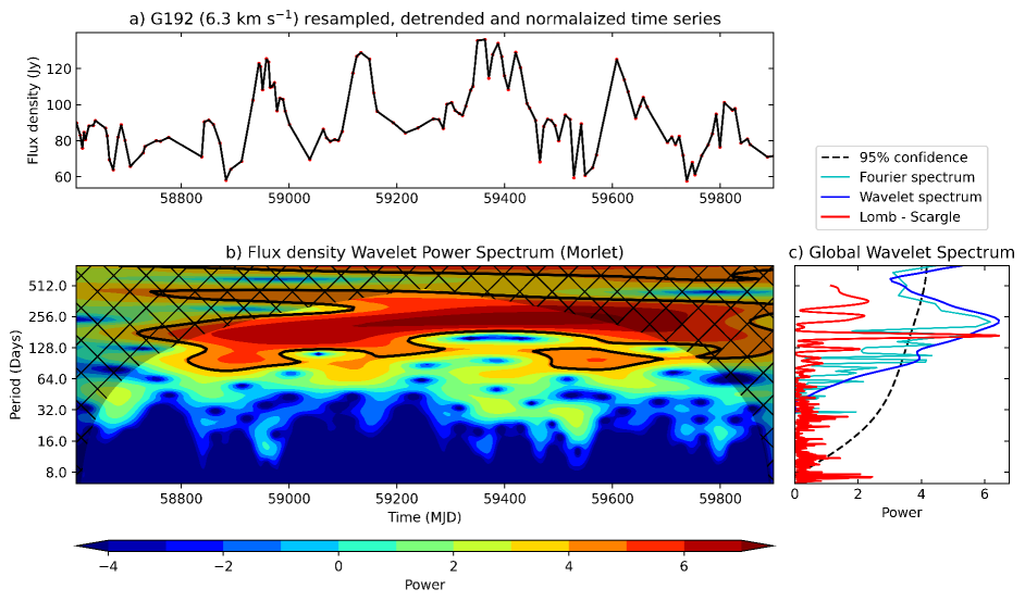
Figure 5: Same as Figure 2., but for the G192.60-0.05 6.3 km s^-1 line. Note, only data obtained alter 58600 (March 2018) MJD were used.

4 DISCUSSION

4.1 Comparison with relevant studies

The variability of 6.7 GHz methanol masers has been a focal point in multiple studies. However, these studies often focus on one or a few sources (e.g. Araya et al. 2010; Szymczak et al. 2016; Olech et al. 2019) or are large surveys that observe each source only a handful of times (e.g. Caswell et al. 1995 and Breen et al. 2015). As previously mentioned, the two most significant long-term studies on 6.7 GHz methanol maser variability, in our opinion, have been conducted by Goedhart et al. (2004) and Szymczak et al. (2018).

In our opinion, only these studies (Goedhart et al. 2004; Yonekura et al. 2016; Szymczak et al. 2018) with their corresponding methanol maser programs are reasonably comparable to ours based on both the large number of target sources and the comparatively high average observation cadence. A comparison with these studies is summarised in Table 5. There is practically no time overlap between all four studies, although it is likely that all teams are continuing 6.7 GHz methanol maser monitoring programs, and, in the future, direct time series comparisons and combinations will be possible. A high percentage of our sample sources were also monitored by Szymczak et al. (2018) and Yonekura et al. (2016), with Goedhart et al. (2004) having a comparably smaller overlap percentage due to Hartebeesthoek radio observatory being located far South.

Our methanol maser monitoring program has a comparable average observation cadence to (Yonekura et al., 2016) and an observation cadence 1.5 to 6 times more frequent than Goedhart et al. (2004) and Szymczak et al. (2018). There is a notable difference in the percentage of detected highly-variable spectral components which have a variability index above 0.5 (see Table 5, eighth line), but this difference can be explained by selection effects; we favoured high flux density sources, which tend to be less variable, according to Szymczak et al. (2018). Concluding, the quantitative characteristics of maser variability are in agreement with Goedhart et al. (2004) and Szymczak et al. (2018), and our work and theirs are complementary.

Table 5: Comparison with the studies by Goedhart et al. (2004); Szymczak et al. (2018) and Sugiyama et al. (2019a).

	Goedhart et al. (2004)	Szymczak et al. (2018)	Sugiyama et al. (2019a)	This work
Start of monitoring program	Jan 1999	Jun 2009	Dec 2012	Mar 2017
End of the examined period	Mar 2003	Feb 2013	Nov 2016	Oct 2022
Duration of monitoring (yr)	4.2	3.7	3.9	5.3
Number of sources	54	137	442	42
Percentage of sample overlap to ours	24	90	97	-
Average observation cadence per month	2-4	1	6-8	6.5
Percentage of periodic sources	13	7	10	19
Percentage of high variable features	55	54	*	28
Percentage of low-variable sources	19	21	*	21

* Unknown value

4.2 Instrument performance

We the utilised ample availability of telescope time to obtain densely sampled time series data for particularly intriguing maser sources. Our high cadence even permitted obtaining four flux density measurements in one hour for a full-week (Figure 3.), which maybe challenging or impossible for many other radio observatories. As mentioned before, the vast majority (95 per cent) of the observations where made with the RT–16. Although telescope parameters are good for a 16 meter antenna, it cannot mach Torun’s 32 meter telescope (Szymczak et al., 2018) in sensitivity. Our monitoring results for sources with low fluxes are more affected by scattering caused by a lower signal to noise ratio.

Our calibration error is comparably high, with relative amplitude precision around 20 per cent. In our view, these variations are not attributed to major flaws in the employed methods or instruments, but rather stems from specific challenges posed by seasonal weather conditions. Irbene is situated a mere 4.2 km from the Baltic Sea, causing rapid fluctuations in telescope gain due to changing weather patterns. The winter season presents the most dynamic and demanding conditions, as the Baltic Sea remains ice-free, and prevailing winds come from the sea, resulting in nearly 100 percent humidity for several months. These periods of high scattering can be noticed in all of the obtained time series. Inability to rapidly and accurately compensate for a changing signal gain is the main factor of high amplitude errors. Due to sporadic results of gain measurements in bad weather conditions, average values were used. Data suffering large deviations from expected gain values were discarded.

4.3 Source variability

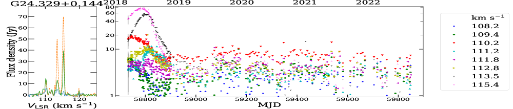
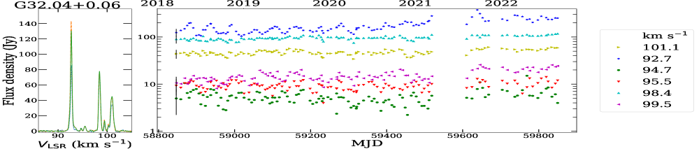
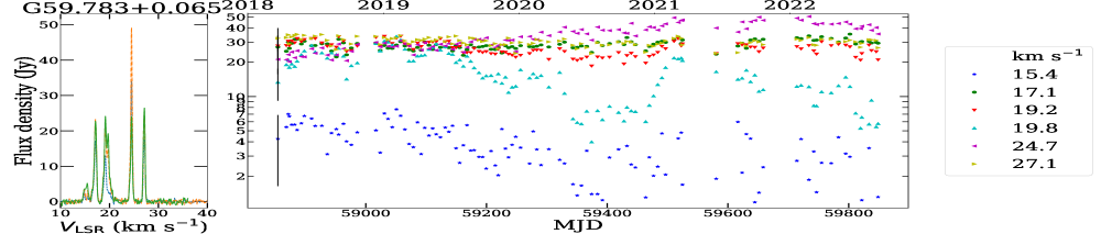
Figure 6: Same as Figure 1., but for the G24.329+0.144; G32.04+0.06 and G59.783+0.065.

No new types of variability were discovered in our observation sample; however, it is worth noting that several sources exhibited changes in their typical variability behaviour. Even sources that were previously considered stable can quickly become variable (e.g., G78.122+3.633/IRAS 20126+410 after a 500-day quiescence period, as shown in Aberfelds et al. 2023) and, conversely, highly variable sources (like G192.60-0.05/S255IR see Figure 1, bottom) can transition to a low-variability state. Notably, the three components of G59.783+0.065 (Figure 6, bottom) became significantly variable after a year-long period of low variability, displaying distinct variability profiles. It is important to emphasise that the variability changes discussed in this paragraph are not related to flares.

4.4 Periodic masers

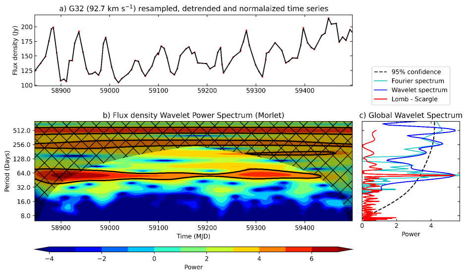
Figure 7: Same as Figure 2., but for the G32.04+0.06 92.7 km s^-1 line. Note, only data obtained until 59500 MJD (October 2021) were used.

Eight sources from our sample (19 percent) exhibit noticeable periodic (cyclic) variations in flux density, but most of them have been previously identified by different research groups (see summary in Table 3.). Our results for the G192.60-0.05 6.3 km s^-1 line (Figure 1, bottom and Figure 5.) and G32.04+0.06 92.7 km s^-1 line (Figure 6, middle and Figure 7.), and G33.641-0.228 61.0 km s^-1 line (Figure 1. middle and Figure 4.), may indicate regularities (periods), previously not reported in the literature. Notably, these potential periodic signals arise from individual spectral features, which is somewhat rarer than the periodic variability of an entire source’s spectra. Additionally, their relative flux increase (percentage by which minimal amplitude increased during cycle) are comparatively lower compared to already known periodic sources (see Table 3.). This highlights that a high observation cadence combined with methods like wavelet analysis, FFT, and the Lomb-Scargle periodogram may enable the detection of period signals with lower relative flux increases compared to already known periods reported in the literature regarding 6.7 GHz methanol maser variability.

The longest cycle of a periodic signal we observed was 500 days (G33.641-0.228). Results of even longer-period variability in G33.641-0.228; G196.454-01.67 and G188.95+0.89/S252 were previously noted in the literature (Goedhart et al. 2004; Olech et al. 2019); however, we didn’t see concrete evidence of these during our observations. The shortest cyclic behaviour was 34.4 days (Figures 1, top and 2.) for G107.298+5.63, which is a well–studied source (Szymczak et al., 2016). We would like to add that sources exhibiting alternately raising and dimming flux densities may indicate long-period cyclical variability. However, to confirm any hypothesis of this pattern, much longer monitoring over an extended time span would be necessary.

4.5 Maser flares

Flares were detected in 10 per cent of sources from our sample (see examples in Figure 1, top and middle and Figure 6, top), all which are already identified events in the literature. New short flaring (flickering) events for the G33.641-0.228 59.6 km s^-1 line (Figure 1, middle) were detected and continued during our monitoring program, although frequency and amplitudes were typically lower than was reported by Fujisawa et al. (2014b). We did daily observations during the G24.329+0.144 flare (Wolak et al., 2019) (see Figure 6, top). During the flare, all spectral components exhibited elevated flux levels by factors from 3 to 10. As noted previously, this flare was similar to the one observed 8 years before (Szymczak et al., 2018), making the G24.329+0.144 an interesting case – which, to our knowledge, is the first object where a strong, long lasting flare has repeated. This source is of great interest for the Maser Monitoring Organization, and follow–up publications using different data from arrays, like Hirota et al. (2022) and Kobak et al. (2023) hopefully will follow.

Most of the periodic and flaring sources in our sample exhibit time lags between different spectral components. This phenomenon is most prominent close to maximum and minimum points. In our sample this is best illustrated in Figures 3. and 6, top.

To identify plausible flares, we suggest the following criteria: the flux measurement should exceed the rolling mean flux (excluding flux measurement’s at suspected flare) by at least five standard deviations (4). Here, $S$ represents the flux, $\overline{S}_{r}$ stands for the rolling mean flux, and $\sigma_{r}$ represents the standard deviation for rolling data. Potential flares can be selected manually or by applying a Z-score test, which involves selecting measurements with scores exceeding 3. Alternatively, other outlier-detection methods may also prove useful. The optimal number of data points to use for calculating the rolling mean and standard deviation can vary depending on the observation intervals and the length of the time series. However, we recommend a minimum of 4 data points, and based on our sample, we have found that using 8 to 14 points demonstrates a high success of identifying maser flares in our sample without giving a false positive for periodic sources.

$$\centering S>\overline{S}_{r}+5\sigma_{r}\@add@centering$$ (4)

To identify the onset of a current flare (one occurring at the present moment), the approach described may not be the most suitable, as it lacks information about the duration and magnitude of the flux increase, and there is no data available for post-flare conditions. In this regard, an empirical approach that defines a flare as a rapid and substantial increase in flux can be more useful. In our opinion, the threshold for identifying a flare can still be determined using the suggested approach by evaluating whether the flux increase still exceeds the recent mean flux density and is five times its standard deviation.

4.6 Velocity drift masers

Only a single source, G121.298+0.659, shows a noticeable velocity drift of the spectral components in the obtained variability time series (Figure 8.). We observed the spectral component at -25.8 km s^-1 drifting towards the -24.9 km s^-1 line and merging with it. This process took approximately 500 days, during which the peak flux of the resulting spectral line increased by 30 to 50 percent compared to the initial peak flux density. This may indicate that we observed only the addition of fluxes from individual maser clouds in the velocity domain and not their amplification by positional alignment along the line of sight in the spatial domain (like observed in Orion KL Shimoikura et al. 2005 and G25.65+1.05 Burns et al. 2019).

Overall, all used variability parameters (variability index, fluctuation index, and $\chi^{2}_{r}$ parameter) show a noticeable positive correlation. In other words, the most variable sources (with high variability indexes) also exhibit the highest fluctuations and possess high $\chi^{2}_{r}$ parameters. Source flux density is negatively correlated with variability parameters, meaning that brighter sources tend to be less variable. This result was expected and is in agreement with Szymczak et al. (2018). Variability amplitudes and trends in maser sources appear to be equally frequently shared among all spectral components or are equally often unique to individual lines. Typically, prolonged periods of flux decline or increase occur alternately, possibly indicating long source cycles. The findings of our results, including high variability with practically the same spectral components, time delays between light curve extremes, and nearly unnoticeable spectral line velocity changes over five years, strongly support the consensus idea that most of the observed 6.7 GHz methanol maser variability is caused by variations in pumping rates.

5 Conclusions

We present the results of a 5-year maser monitoring campaign for 42 sources of 6.7 GHz methanol masers, observed with two radio telescopes located in North West Latvia. Our data on well–known sources show mostly a continuation of previously identified variability trends. Several new variability trends for separate sources were found: possibly periodic fluctuations of G192.60-0.05 and G32.04+0.06; initiation of rapid variability in G78.122+3.633 and G59.783+0.065. Summarising the data also highlighted particular seasonal weather challenges, which are not fully compensated with methods we employed. Due to these limitations, only high amplitude ($\geq 30$ per cent) variability can reliably be studied with our telescopes. Our team is committed to enhance the capabilities and accuracy of our facility. These maser monitoring results can be used to select potentially interesting sources for detailed studies using VLBI techniques.

Data Availability

All source spectra with reasonable request can obtained thought private communication with corresponding author. Time series plots for all other sources are available in the article and in its online supplementary material.

Appendix A Additional time series

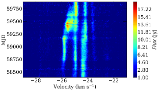
Figure 8: Dynamic spectra of G121.298+0.659 illustrating velocity drifting.

Appendix B Full variability parameter table

Full table of maser line variability parameters, same information as in Table 4 V_P(km s^-1) S_P(Jy) $VI$ $FI$ $\chi^{2}_{r}$
Continued from previous column
V_P(km s^-1) S_P(Jy) $VI$ $FI$ $\chi^{2}_{r}$
Continued on next column
Concluded l c c c l G22.357+0.066 (MJD_s=58220, $T\textsubscript{s}$= 4.462 y, $N$=202)
78.7 2.60 0.74 0.70 0.84
80.1 18.49 0.40 0.46 1.11
88.3 2.83 0.58 0.53 0.59
G24.329+0.144 (MJD_s=58731, $T\textsubscript{s}$= 3.060 y, $N$=236)
108.2 2.12 0.19 0.64 0.37
109.4 2.82 0.47 0.57 0.42
110.2 9.30 0.73 0.49 1.96
111.2 4.70 0.61 0.66 1.05
111.8 4.13 0.76 0.41 0.36
112.8 5.58 0.80 0.62 1.22
113.5 18.73 0.94 1.50 33.70
115.4 23.76 0.88 1.90 58.40
G25.709+0.044 (MJD_s=58846, $T\textsubscript{s}$= 2.751 y, $N$=108)
89.8 50.14 0.04 0.09 0.15
91.3 12.65 0.16 0.22 0.27
92.0 26.63 0.07 0.14 0.20
93.3 43.55 -0.05 0.17 0.28
94.0 64.57 -0.03 0.12 0.24
95.5 321.65 -0.04 0.06 0.22
95.7 328.85 -0.01 0.07 0.17
97.9 7.48 0.12 0.28 0.15
G25.64+1.05 (MJD_s=58024, $T\textsubscript{s}$= 5.003 y, $N$=253)
38.6 2.42 0.43 0.89 0.34
40.3 4.38 0.15 0.56 0.34
41.8 129.75 0.07 0.17 0.99
42.5 3.06 0.35 0.58 0.36
G30.99-0.08 (MJD_s=57950, $T\textsubscript{s}$= 5.202 y, $N$=248)
74.8 7.91 0.01 0.36 0.81
77.8 12.69 0.45 0.59 3.48
88.4 4.87 0.63 0.61 1.55
G32.04+0.06 (MJD_s=58846, $T\textsubscript{s}$= 2.748 y, $N$=117)
101.1 47.37 0.10 0.16 0.35
92.7 172.25 0.40 0.50 2.50
94.7 5.36 0.47 0.51 0.45
95.5 9.30 0.23 0.28 0.39
98.4 96.06 0.07 0.07 0.28
99.5 15.12 0.25 0.38 0.76
G32.744-0.076 (MJD_s=57825, $T\textsubscript{s}$= 5.596 y, $N$=1016)
30.5 15.01 -0.04 0.14 0.15
32.1 30.67 0.15 0.06 0.43
33.5 38.56 0.01 0.08 0.23
38.1 37.89 0.09 0.11 0.26
38.3 40.43 0.10 0.04 0.21
38.5 42.97 0.03 0.07 0.26
39.2 16.88 0.09 0.07 0.17
G33.641-0.228 (MJD_s=57821, $T\textsubscript{s}$= 5.707 y, $N$=1136)
59.3 18.78 0.83 1.05 17.86
59.6 15.40 0.73 0.77 2.18
60.3 161.73 0.21 0.50 2.66
61.0 49.98 0.49 0.65 4.56
62.7 18.39 0.32 0.18 0.56
63.2 15.21 0.39 0.16 0.28
G35.20-1.74 (MJD_s=57956, $T\textsubscript{s}$= 5.186 y, $N$=277)
41.0 3.11 0.81 0.58 1.50
43.1 23.70 0.19 0.30 0.66
43.8 14.15 0.62 0.45 5.42
44.1 11.79 0.52 0.34 2.08
44.6 35.31 0.08 0.18 0.33
44.9 25.62 0.14 0.18 0.73
45.3 17.51 0.02 0.26 0.54
G34.396+0.222 (MJD_s=58312, $T\textsubscript{s}$= 4.210 y, $N$=204)
55.6 24.10 0.42 0.52 2.34
62.5 5.55 0.17 0.27 0.25
G36.705+0.096 (MJD_s=58289, $T\textsubscript{s}$= 4.273 y, $N$=191)
62.2 2.56 0.25 0.43 0.41
G37.479-0.105 (MJD_s=57881, $T\textsubscript{s}$= 5.393 y, $N$=256)
50.0 2.58 -0.31 0.17 0.55
52.3 1.87 -0.51 0.54 0.41
56.9 9.47 -0.06 0.18 0.32
58.3 4.85 -0.07 0.05 0.47
59.3 4.90 -0.16 0.25 0.24
60.1 1.99 0.21 0.46 0.29
62.0 9.11 0.13 0.35 0.28
62.5 7.38 -0.06 0.38 0.26
G37.43+1.52 (MJD_s=58846, $T\textsubscript{s}$= 2.748 y, $N$=111)
41.3 360.69 0.03 0.10 0.21
G37.55+0.20 (MJD_s=58298, $T\textsubscript{s}$= 4.246 y, $N$=198)
83.8 6.25 0.40 0.56 1.13
84.8 5.81 0.20 0.42 0.73
86.4 3.60 0.28 0.34 0.51
G43.149+0.013 (MJD_s=57881, $T\textsubscript{s}$= 5.398 y, $N$=265)
13.2 16.11 -0.04 0.15 0.18
18.9 20.51 -0.06 0.14 0.30
19.6 12.24 0.16 0.32 0.33
20.2 8.53 0.03 0.23 0.28
8.4 16.17 -0.02 0.22 0.23
9.3 37.00 0.03 0.19 0.29
G43.796-0.127 (MJD_s=58319, $T\textsubscript{s}$= 4.189 y, $N$=204)
39.6 15.97 0.18 0.16 0.41
40.0 16.71 0.14 0.15 0.47
40.4 19.48 0.00 0.08 0.30
43.0 15.27 0.03 0.15 0.23
G45.071+0.013 (MJD_s=58854, $T\textsubscript{s}$= 2.724 y, $N$=112)
57.8 40.06 -0.12 0.10 0.16
G49.04-1.08 (MJD_s=58389, $T\textsubscript{s}$= 1.251 y, $N$=61)
35.6 14.25 0.14 0.20 0.95
36.5 8.49 0.24 0.13 0.46
37.1 13.47 0.46 0.34 2.96
38.4 4.53 0.65 1.12 5.25
39.2 5.99 0.57 0.65 3.96
40.9 1.43 0.53 0.67 1.10
G196.454-01.67 (MJD_s=58842, $T\textsubscript{s}$= 2.774 y, $N$=88)
14.7 13.85 0.60 0.76 2.85
15.2 10.64 0.35 0.42 0.89
15.5 10.26 0.52 0.59 1.56
G49.490-0.388 (MJD_s=57885, $T\textsubscript{s}$= 5.388,
$N$=297, $C(month^{-1})$=4.594)
50.1 11.87 0.19 0.23 0.21
51.8 55.05 0.03 0.22 0.34
56.2 39.85 0.04 0.25 0.44
57.9 128.99 0.22 0.22 1.61
58.3 147.05 0.02 0.23 0.83
58.8 274.17 0.41 0.49 5.37
59.3 842.08 0.00 0.14 0.49
G192.60-0.05 (MJD_s=57856, $T\textsubscript{s}$= 5.476 y, $N$=368)
2.3 7.28 0.92 2.52 8.39
4.2 7.17 0.67 0.79 1.71
4.8 15.74 0.63 0.75 2.56
5.9 176.49 0.37 0.52 3.05
6.3 162.01 0.81 1.59 17.18
7.5 4.51 0.97 4.24 6.32
G189.030+0.784 (MJD_s=57839, $T\textsubscript{s}$= 2.567 y, $N$=155)
8.8 16.80 0.55 0.12 1.03
9.6 14.55 0.28 0.28 2.48
G59.783+0.065 (MJD_s=58854, $T\textsubscript{s}$= 2.724 y, $N$=113)
15.4 3.62 0.56 0.60 0.98
17.1 28.46 -0.05 0.12 0.14
19.2 26.52 -0.02 0.26 0.31
19.8 16.44 0.59 0.79 4.60
24.7 33.57 0.21 0.38 1.17
27.1 30.28 -0.08 0.15 0.13
G69.540-0.976 (MJD_s=57832, $T\textsubscript{s}$= 5.530 y, $N$=206)
0.0 6.54 0.42 0.19 0.47
1.3 3.95 0.16 0.51 0.35
14.6 112.12 0.15 0.16 0.44
G174.20-0.08 (MJD_s=57832, $T\textsubscript{s}$= 5.542 y, $N$=261)
1.4 43.69 0.50 0.37 3.88
3.8 9.27 0.60 0.56 3.30
4.6 5.19 0.15 0.24 0.40
G173.482+2.446 (MJD_s=57821, $T\textsubscript{s}$= 5.572 y, $N$=250)
-11.8 6.78 0.18 0.40 0.49
-13.0 25.46 0.36 0.29 1.57
-13.8 18.91 0.15 0.43 1.02
-7.5 9.86 0.41 0.73 3.78
G73.06+1.80 (MJD_s=58859, $T\textsubscript{s}$= 2.709 y, $N$=137)
-2.7 1.65 0.68 0.76 0.67
6.0 7.42 0.36 0.55 1.20
G75.782+0.343 (MJD_s=57885, $T\textsubscript{s}$= 5.379 y, $N$=313)
-0.1 4.86 0.68 0.58 2.18
-0.4 6.68 0.35 0.28 0.92
-2.6 63.86 0.14 0.04 0.69
0.7 25.71 0.42 0.22 2.35
G78.122+3.633 (MJD_s=57832, $T\textsubscript{s}$= 5.549 y, $N$=882)
-6.1 27.70 0.24 0.20 0.61
-6.7 29.15 0.74 0.67 11.66
-7.0 18.42 0.62 0.64 4.87
-7.7 24.06 0.97 2.48 65.51
G81.88+0.78 (MJD_s=57834, $T\textsubscript{s}$= 5.525 y, $N$=300)
3.5 83.53 0.33 0.42 1.34
4.1 219.65 0.38 0.47 1.92
4.6 311.00 0.16 0.27 0.80
5.2 105.18 0.17 0.22 0.57
5.8 99.84 0.15 0.24 0.62
7.3 264.17 0.34 0.37 1.92
9.5 36.10 0.52 0.66 2.87
G188.95+0.89 (MJD_s=57993, $T\textsubscript{s}$= 5.101 y, $N$=223)
10.5 478.64 0.28 0.23 1.60
10.8 868.89 0.11 0.32 1.30
11.6 13.51 0.46 0.37 1.18
11.8 8.32 0.71 0.52 2.88
8.5 6.88 0.17 0.28 0.36
9.7 39.52 0.06 0.29 0.75
G85.411+0.002 (MJD_s=58842, $T\textsubscript{s}$= 2.832 y, $N$=698)
-28.6 5.15 0.34 0.38 0.38
-29.4 84.99 0.01 0.16 0.21
-30.8 3.98 0.36 0.37 0.32
-31.6 90.06 0.40 0.38 3.08
-33.0 2.42 0.04 0.60 0.40
G90.925+1.486 (MJD_s=57885, $T\textsubscript{s}$= 5.379 y, $N$=305)
-69.2 61.49 0.36 0.44 3.99
-70.4 29.79 0.37 0.39 1.60
G94.602-1.796 (MJD_s=58027, $T\textsubscript{s}$= 4.996 y, $N$=351)
-40.9 5.30 0.14 0.45 0.68
-43.0 2.88 0.73 0.26 0.43
-43.7 3.74 0.43 0.47 0.59
G173.482+2.446 (MJD_s=57821, $T\textsubscript{s}$= 5.572 y, $N$=250)
-11.8 6.78 0.18 0.40 0.49
-13.0 25.46 0.36 0.29 1.57
-13.8 18.91 0.15 0.43 1.02
-7.5 9.86 0.41 0.73 3.78
G111.26-0.77 (MJD_s=57828, $T\textsubscript{s}$= 5.535 y, $N$=315)
-36.0 0.68 0.76 1.36 0.35
-38.0 1.64 0.59 0.66 0.69
G111.542+0.777 (MJD_s=57832, $T\textsubscript{s}$= 5.541 y, $N$=276)
-48.2 10.62 0.34 0.39 1.03
-48.8 9.82 0.40 0.40 1.15
-56.1 74.46 0.37 0.26 3.11
-56.8 103.97 0.14 0.31 0.62
-57.6 177.57 0.16 0.35 1.14
-58.0 247.68 0.19 0.31 0.72
-60.7 130.11 0.11 0.29 0.56
-61.3 165.87 0.20 0.44 1.70
G133.947+1.064 (MJD_s=57841, $T\textsubscript{s}$= 5.520 y, $N$=297)
-41.8 40.17 0.41 0.49 2.13
-42.2 289.10 0.62 1.25 10.33
-42.6 1376.89 0.29 0.33 2.45
-43.0 2230.47 0.12 0.36 1.25
-43.5 2800.11 0.11 0.33 1.15
-44.6 3366.63 0.11 0.33 1.14
-45.1 2612.50 0.12 0.35 1.27
-45.5 2090.53 0.09 0.29 1.02
G109.871+2.114 (MJD_s=57829, $T\textsubscript{s}$= 5.684 y, $N$=1504)
-1.8 225.67 0.45 0.72 18.04
-2.4 1026.05 0.59 0.83 50.19
-3.7 265.84 0.41 0.43 5.41
-4.0 418.37 0.18 0.30 1.17
-4.7 23.86 0.85 0.89 15.04
G121.298+0.659 (MJD_s=57841, $T\textsubscript{s}$= 5.605 y, $N$=289)
-22.4 1.86 0.67 0.44 0.64
-24.4 8.08 0.44 0.51 1.36
-24.9 7.72 0.85 1.00 10.55
-25.8 5.09 0.87 1.74 6.74
-27.0 1.70 0.34 0.51 0.39
-27.5 1.43 0.64 0.43 0.57
G107.298+5.639 (MJD_s=58298, $T\textsubscript{s}$= 4.285 y, $N$=1823)
-11.0 1.53 0.61 0.81 1.10
-16.7 1.71 0.91 3.09 1.96
-7.4 27.04 0.99 4.81 307.60
-8.6 4.30 0.88 1.76 8.21
-9.2 7.46 0.98 6.76 23.56
G108.184+5.519 (MJD_s=57839, $T\textsubscript{s}$= 5.523 y, $N$=282)
-10.0 17.20 0.58 0.36 4.33
-10.8 33.57 0.40 0.18 3.65
-12.7 15.56 0.36 0.47 1.12

References

- Aberfelds et al. (2017) Aberfelds A., Shmeld I., Berzins K., 2017, Proceedings of the International Astronomical Union, 13, 277
- Aberfelds et al. (2021) Aberfelds A., Steinbergs J., Shmeld I., Bartkiewicz A., 2021, Astronomical and Astrophysical Transactions, 32, 383
- Aberfelds et al. (2023) Aberfelds A., Bartkiewicz A., Szymczak M., Šteinbergs J., Surcis G., Kobak A., Durjasz M., Shmeld I., 2023, MNRAS, 524, 599
- Aller et al. (2003) Aller M. F., Aller H. D., Hughes P. A., 2003, ApJ, 586, 33–51
- Antyufeyev et al. (2020) Antyufeyev O., et al., 2020, Astronomical and Astrophysical Transactions, 32, 23
- Araya et al. (2010) Araya E. D., Hofner P., Goss W. M., Kurtz S., Richards A. M. S., Linz H., Olmi L., Sewiło M., 2010, ApJ, 717, L133
- Bleiders et al. (2017) Bleiders M., Bezrukovs V., Orbidans A., 2017, Latvian Journal of Physics and Technical Sciences, 54, 42
- Bleiders et al. (2020) Bleiders M., Antyufeyev O., Patoka O., Orbidans A., Aberfelds A., Steinbergs J., Bezrukovs V., Shmeld I., 2020, Journal of Astronomical Instrumentation, 09, 2050009
- Breen et al. (2015) Breen S. L., et al., 2015, MNRAS, 450, 4109
- Burns et al. (2019) Burns R. A., et al., 2019, Monthly Notices of the Royal Astronomical Society, 491, 4069
- Burns et al. (2020) Burns R. A., et al., 2020, Nature Astronomy, 4, 506
- Caratti o Garatti et al. (2017) Caratti o Garatti A., et al., 2017, Nature Physics, 13, 276
- Caswell et al. (1995) Caswell J. L., Vaile R. A., Ellingsen S. P., 1995, Publ. Astron. Soc. Australia, 12, 37
- Durjasz et al. (2019) Durjasz M., Szymczak M., Olech M., 2019, MNRAS, 485, 777
- Fujisawa et al. (2014a) Fujisawa K., et al., 2014a, PASJ, 66, 78
- Fujisawa et al. (2014b) Fujisawa K., et al., 2014b, PASJ, 66
- Fujisawa et al. (2015) Fujisawa K., Yonekura Y., Sugiyama K., Horiuchi H., Hayashi T., Hachisuka K., Matsumoto N., Niinuma K., 2015, The Astronomer’s Telegram, 8286, 1
- Goddi et al. (2011) Goddi C., Moscadelli L., Sanna A., 2011, A&A, 535, L8
- Goedhart et al. (2004) Goedhart S., Gaylard M. J., van der Walt D. J., 2004, MNRAS, 355, 553
- Goedhart et al. (2014) Goedhart S., Maswanganye J. P., Gaylard M. J., van der Walt D. J., 2014, MNRAS, 437, 1808
- Gray (2012) Gray M., 2012, Maser Sources in Astrophysics. Cambridge Astrophysics, Cambridge University Press, doi:10.1017/CBO9780511977534
- Himwich (2000) Himwich E., 2000, in Takahashi F., ed., International VLBI Service for Geodesy and Astrometry 2000 General Meeting Proceedings. pp 86–90
- Hirota et al. (2022) Hirota T., et al., 2022, PASJ, 74, 1234
- Inayoshi et al. (2013) Inayoshi K., Sugiyama K., Hosokawa T., Motogi K., Tanaka K. E. I., 2013, ApJ, 769, L20
- Kobak et al. (2023) Kobak A., et al., 2023, A&A, 671, A135
- Liu et al. (2007) Liu Y., San Liang X., Weisberg R. H., 2007, Journal of Atmospheric and Oceanic Technology, 24, 2093
- MacLeod et al. (2018) MacLeod G. C., et al., 2018, MNRAS, 478, 1077
- Menten (1991) Menten K. M., 1991, ApJ, 380, L75
- Moscadelli et al. (2017) Moscadelli L., et al., 2017, A&A, 600, L8
- Olech et al. (2019) Olech M., Szymczak M., Wolak P., Sarniak R., Bartkiewicz A., 2019, MNRAS, 486, 1236
- Olech et al. (2020) Olech M., Szymczak M., Wolak P., Gérard E., Bartkiewicz A., 2020, A&A, 634, A41
- Olech et al. (2022) Olech M., Durjasz M., Szymczak M., Bartkiewicz A., 2022, A&A, 661, A114
- Parfenov & Sobolev (2014) Parfenov S. Y., Sobolev A. M., 2014, MNRAS, 444, 620
- Perley & Butler (2013) Perley R. A., Butler B. J., 2013, A&AS, 204, 19
- Ryabov & Vrublevskis (2023) Ryabov B., Vrublevskis A., 2023, Latvian Journal of Physics and Technical Sciences, 60, 52
- Salii et al. (2022) Salii S. V., Zinchenko I. I., Liu S.-Y., Sobolev A. M., Aberfelds A., Su Y.-N., 2022, MNRAS, 512, 3215
- Scargle (1982) Scargle J. D., 1982, ApJ, 263, 835
- Sebastian et al. (2023) Sebastian K., Nabil F., Alexey B., Christopher T., Gilbert P. C., 2023, PyCWT, https://github.com/regeirk/pycwt
- Shimoikura et al. (2005) Shimoikura T., Kobayashi H., Omodaka T., Diamond P. J., Matveyenko L. I., Fujisawa K., 2005, The Astrophysical Journal, 634, 459
- Stecklum et al. (2021) Stecklum B., et al., 2021, A&A, 646, A161
- Steinbergs et al. (2021) Steinbergs J., Aberfelds A., Bleiders M., Shmeld I., 2021, VIRAC maser data processing suite, https://doi.org/10.17184/eac.5643
- Stetson (1996) Stetson P. B., 1996, PASP, 108, 851
- Sugiyama et al. (2019a) Sugiyama K., et al., 2019a, Journal of Physics: Conference Series, 1380, 012057
- Sugiyama et al. (2019b) Sugiyama K., Saito Y., Yonekura Y., Momose M., 2019b, The Astron. Telegr., 12446, 1
- Sukharev et al. (2022) Sukharev A., Ryabov M., Bezrukovs V., Orbidans A., 2022, Astronomical and Astrophysical Transactions, 33, 149
- Szymczak et al. (2011) Szymczak M., Wolak P., Bartkiewicz A., van Langevelde H. J., 2011, A&A, 531, L3
- Szymczak et al. (2012) Szymczak M., Wolak P., Bartkiewicz A., Borkowski K. M., 2012, Astronomische Nachrichten, 333, 634
- Szymczak et al. (2014) Szymczak M., Wolak P., Bartkiewicz A., 2014, MNRAS, 439, 407
- Szymczak et al. (2015) Szymczak M., Wolak P., Bartkiewicz A., 2015, MNRAS, 448, 2284
- Szymczak et al. (2016) Szymczak M., Olech M., Wolak P., Bartkiewicz A., Gawroński M., 2016, MNRAS, 459, L56–L60
- Szymczak et al. (2018) Szymczak M., Olech M., Sarniak R., Wolak P., Bartkiewicz A., 2018, MNRAS, 474, 219
- Torrence & Compo (1998) Torrence C., Compo G. P., 1998, Bulletin of the American Meteorological Society, 79, 61
- Virtanen et al. (2020) Virtanen P., et al., 2020, Nature Methods, 17, 261
- Walsh et al. (1998) Walsh A. J., Burton M. G., Hyland A. R., Robinson G., 1998, MNRAS, 301, 640
- Winkel et al. (2012) Winkel B., Kraus A., Bach U., 2012, A&A, 540, A140
- Wolak et al. (2019) Wolak P., Olech M., Szymczak M., Bartkiewicz A., Durjasz M., 2019, The Astronomer’s Telegram, 13080, 1
- Yonekura et al. (2016) Yonekura Y., et al., 2016, Publications of the Astronomical Society of Japan, 68, 74
- Younes et al. (2022) Younes G., et al., 2022, ApJ, 924, 136
- Zinnecker & Yorke (2007) Zinnecker H., Yorke H. W., 2007, ARA&A, 45, 481
- van der Walt (2011) van der Walt D. J., 2011, ApJ, 141, 152
- van der Walt et al. (2007) van der Walt D. J., Sobolev A. M., Butner H., 2007, A&A, 464, 1015