Variant Codes Based on A Special Polynomial Ring and Their Fast Computations

Abstract

In this paper, we propose two new classes of binary array codes, termed V-ETBR and V-ESIP codes, by reformulating and generalizing the variant technique of deriving the well-known generalized row-diagonal parity (RDP) codes [1] from shortened independent parity (IP) codes [2]. The V-ETBR and V-ESIP codes are both based on binary parity-check matrices and are essentially variants of two classes of codes over a special polynomial ring (termed ETBR and ESIP codes in this paper).

To explore the conditions that make the variant codes binary Maximum Distance Separable (MDS) array codes that achieve optimal storage efficiency, this paper derives the connections between V-ETBR/V-ESIP codes and ETBR/ESIP codes. These connections are beneficial for constructing various forms of the variant codes. By utilizing these connections, this paper also explicitly presents the constructions of V-ETBR and V-ESIP MDS array codes with any number of parity columns $r$, along with their fast syndrome computations. In terms of construction, all proposed MDS array codes have an exponentially growing total number of data columns with respect to the column size, while alternative codes have that only with linear order. In terms of computation, the proposed syndrome computations make the corresponding encoding/decoding asymptotically require $\lfloor\lg r\rfloor+1$ XOR (exclusive OR) operations per data bit, when the total number of data columns approaches infinity. This is also the lowest known asymptotic complexity in MDS codes [3].

I Introduction

Modern distributed storage systems require data redundancy to maintain data reliability and durability in the presence of unpredictable failures. Replications and erasure codes are two typical redundancy mechanisms [4]. Compared to the former, erasure codes only need less data redundancy to attain the same level of data protection [5]. One well-known class of erasure codes is binary array codes [6, 2, 1, 7]. Their coding procedures involve only XOR (exclusive OR) and cyclic shift operations, which enables simple and efficient implementations in both software and hardware [8]. This paper focuses on such codes.

Binary array codes have been widely used in storage systems, such as RAID (Redundant Array of Independent Disks) [9]. With the development of distributed storage systems in recent years, they have also been used as the basis for developing other erasure codes, such as locally repairable codes [8, 10, 4, 11] and regenerating codes [12, 13, 14]. For an $\ell\times(k+r)$ binary array code, any codeword can be viewed as an $\ell\times(k+r)$ array of bits, where $k$ columns store all information bits to form $k$ information columns, and the remaining columns store all the parity bits encoded from information bits to form $r$ parity columns. The column size $\ell$ generally depends on the code construction. In coding theory, maximum distance separable (MDS) codes reach optimal storage efficiency [15] and each of their codewords consists of information and parity symbols, such that any subset of symbols in the codeword with the same number as information symbols can recover the entire codeword. Binary MDS array codes have the same property by treating each column as a symbol. More precisely, for an $\ell\times(k+r)$ binary MDS array code, any $k$ out of $k+r$ columns suffice to decode (reconstruct) all $k$ information columns. Some well-known examples of binary array codes are EVENODD [16], row-diagonal parity (RDP) [17], STAR [18], and triple-fault-tolerance codes [19]. These codes are all binary MDS array codes for the case of two or three parity columns. Examples of binary array codes with more parity columns are Blaum-Roth (BR) [6], Independent-Parity (IP) [2], generalized RDP codes [1], and the codes in [20]. Although they are not always binary MDS array codes, the conditions that render them such codes can be found in the corresponding literature.

The new binary array codes proposed in this paper target an arbitrary number of parity columns, and their constructions are closely related to the above-mentioned BR, IP, and generalized RDP codes. Note that BR and IP codes are both constructed by parity-check matrices over an all-one polynomial (AOP) ring $\frac{\mathbb{F}_{2}[x]}{\langle\sum_{i=0}^{p-1}x^{i}\rangle}$, where $\mathbb{F}_{2}$ denotes a binary field and $p$ is a prime number [6, 2]. Generalized RDP codes can be regarded as a variant of shortened IP codes [1], and they possess lower encoding/decoding complexity [21]. In this paper, we reformulate the generalized RDP codes, and then one can intuitively understand the essence of the generalized RDP codes being more computationally superior. Briefly, when computing syndromes (which dominates the overall computational complexity of encoding/decoding when code rate $k/(k+r)$ is close to one), codes over $\frac{\mathbb{F}_{2}[x]}{\langle\sum_{i=0}^{p-1}x^{i}\rangle}$ are first calculated in an auxiliary polynomial ring $\frac{\mathbb{F}_{2}[x]}{\langle x^{p}+1\rangle}$, where multiplying $x$ only requires performing a simple cyclic-shift operation, and then all results are reduced to the original ring [6, 2]. As a variant, the generalized RDP codes are derived from the shortened IP codes in such a way that bits exceeding the number of bits in each symbol over the original ring are always not processed. Therefore, two operations of the shortened IP codes are eliminated in the generalized RDP codes. One is the processing for one fixed bit in each symbol, and the other is the modulo operation for reducing to the original ring. A binary parity-check matrix for the generalized RDP codes is explicitly provided in this paper (see (11)), which is not given in other literature.

This paper generalizes the above variant technique so that the new codes based on binary parity-check matrices can be easily obtained from the codes over the special polynomial ring $\frac{\mathbb{F}_{2}[x]}{\langle\sum_{i=0}^{p-1}x^{i\tau}\rangle}$, where $p$ is an odd number and $\tau$ is a power of two. The generalization means that $\tau$ is not limited to one, and the parity-check matrices of codes over polynomial rings can be determined not only by the Vandermonde matrices containing only monomials (such as BR, IP codes) but also by a wider range of parameters. In this paper, the codes defined in $\frac{\mathbb{F}_{2}[x]}{\langle\sum_{i=0}^{p-1}x^{i\tau}\rangle}$ are referred to as ETBR and ESIP codes, which can be regarded as extensions of BR and shortened IP codes, respectively. Correspondingly, the variants of ETBR and ESIP codes are referred to as V-ETBR and V-ESIP codes, respectively. The main contributions of this paper are enumerated as follows:

1. This paper reformulates and generalizes the variant technology of deriving generalized RDP codes from shortened IP codes, and then proposes two new classes of binary array codes (i.e., V-ETBR and V-ESIP codes), which are both based on binary parity-check matrices.

2. To obtain the conditions for the new codes to be binary MDS array codes, this paper presents the connections between them and the codes over special polynomial rings (i.e., ETBR and ESIP codes). Note that these connections are built on the foundation that all parity-check matrices have a sufficiently flexible form. This provides convenience for constructing binary MDS array codes.

3. This paper explicitly presents the constructions for the V-ETBR and V-ESIP MDS array codes, both with any number of parity columns $r$. This leads to the corresponding MDS codes over polynomial rings being directly available as by-products. In particular, compared to existing binary MDS array codes, the constructed codes have significantly more data columns for a given design parameter $p$, as well as a more flexible column size $\ell$.

4. This paper also proposes two fast syndrome computations, which respectively corresponds to the constructed V-ETBR MDS array codes with any $r\geq 2$ and the constructed V-ESIP MDS array codes with $r=4$. Both of them make the corresponding encoding/decoding procedure require asymptotically $\lfloor\lg r\rfloor+1$ XORs per data bit when the total number of data columns approaches infinity. This is also the lowest known asymptotic computational complexity in MDS codes [3].

Note that the fast syndrome computations proposed in this paper can be easily adjusted to be suitable for the corresponding codes over polynomial rings. To avoid tediousness, this paper will not repeat the presentation. It is worth mentioning that compared to the ETBR/ESIP codes over polynomial rings, the variant codes (i.e., V-ETBR/V-ESIP codes) have the following two advantages in calculations. One is that the variant technology brings strictly fewer operations in syndrome computations, as described earlier regarding generalized RDP codes. The other is that all variant codes are based on binary parity-check matrices, leading to easy implementation through the use of existing open-source libraries for matrix operations over $\mathbb{F}_{2}$, such as M4RI [22]. Furthermore, it is possible that many existing scheduling algorithms for matrix operations over $\mathbb{F}_{2}$ can be utilized to improve computational efficiency, such as those proposed in [23, 24]. In contrast, the arithmetic implementation of polynomial rings is complex. Recently, [8, 25] proposed some binary array codes that are essentially V-ETBR/V-ESIP codes. However, there are significant differences between their work and that of this paper:

1. This paper clearly reveals the relationship between V-ETBR/V-ESIP codes and the well-known generalized RDP codes, as the former is a generalization of the variant technique implied by the latter. This is not pointed out in [8, 25].

2. In [8, 25], the proposed V-ETBR/V-ESIP codes consider only parity-check matrices determined by Vandermonde matrices. In contrast, the parity-check matrices for V-ETBR/V-ESIP codes have a more flexible form in this paper, of which the Vandermonde matrix is just a special instance. This can facilitate the construction of more variant codes.

3. [8] and [25] focus on V-ETBR/V-ESIP codes alone, without discussing their connections with the codes over polynomial rings. In this paper, we consider these connections and show that, based on them, some new MDS codes over polynomial rings can be directly obtained as by-products.

4. In terms of construction, all V-ETBR and V-ESIP MDS array codes proposed in [8, 25] and this paper can have a total number of data columns far exceeding the design parameter $p$. However, the feasible number of parity columns $r$ for the V-ESIP MDS array codes in [8, 25] is three, while that in this paper is any size.

5. In terms of computation, the fast syndrome computation proposed in [8, 25] is for $2\leq r\leq 3$, whereas that proposed in this paper is for arbitrary $r\geq 2$. The former is actually a special case of the latter.

The remainder of this paper is organized as follows. Section II introduces all necessary preliminaries, including some existing well-known binary array codes and important notations. Section III provides the specific definitions of V-ETBR/V-ESIP and ESIP/ESIP codes. Section IV first presents the connections for V-ETBR/V-ESIP and ESIP/ESIP codes, and then constructs the V-ETBR/V-ESIP MDS array codes. In Section V, some fast syndrome computations for the constructed codes are proposed. Section VI concludes this paper.

II Preliminaries

This section describes some existing well-known classes of array codes, i.e., BR codes [6], IP codes [2], and generalized RDP codes [1]. To begin with, let

$$\mathbb{R}_{p,\tau}:=\frac{\mathbb{F}_{2}[x]}{\langle f_{p,\tau}(x)\rangle}$$ (1)

denote a binary polynomial ring, where

$$f_{p,\tau}(x)=1+x^{\tau}+\cdots+x^{(p-1)\tau}$$ (2)

with two positive integers $p,\tau$. The identity that $x^{p\tau}+1=(x^{\tau}+1)\cdot f_{p,\tau}(x)$ leads to that operations in $\mathbb{R}_{p,\tau}$ can be performed first in polynomial ring

$$\mathbb{R}:=\frac{\mathbb{F}_{2}[x]}{\langle x^{p\tau}+1\rangle},$$ (3)

and then, all results should be reduced modulo $f_{p,\tau}(x)$. Since multiplying by $x$ in $\mathbb{R}$ is equivalent to performing a one-bit cyclic shift on a vector with $p\tau$ bits, the above realization for the operations in $\mathbb{R}_{p,\tau}$ is simple and efficient [6, 2].

II-A BR codes

BR codes are constructed in polynomial ring $\mathbb{R}_{p,1}$ [6], where $p$ is a prime number. Given the value of $p$, the BR$(p,r<p)$ is defined as the set of $(p-1)\times p$ arrays (denoted by $[x_{i,j}]$, where $x_{i,j}\in\{0,1\}$, the first $p-r$ data columns are information columns and others are parity columns). For $\ell=0,1,\cdots,p-1$, the $\ell$-th column of a $(p-1)\times p$ array can be viewed as a binary polynomial $D_{\ell}=\sum_{i=0}^{p-2}x_{i,\ell}\cdot x^{i}\in\mathbb{R}_{p,1}$. The BR$(p,r)$ requires that $0=H_{BR}\cdot(D_{0},D_{1},\cdots,D_{p})^{\mathrm{T}}$, where $H_{BR}\in\mathbb{R}_{p,1}^{r\times n}$ is the Vandermonde parity-check matrix given by

$$H_{BR}=\left(\begin{array}[]{ccccc}1&1&1&\cdots&1\\ 1&x&x^{2}&\cdots&x^{p-1}\\ \vdots&\vdots&\vdots&\ddots&\vdots\\ 1&x^{r-1}&x^{2(r-1)}&\cdots&x^{(r-1)(p-1)}\end{array}\right).$$ (4)

BR codes have an intuitive graphical representation. Figure 2 provides an example of BR$(5,3)$ to demonstrate it. In Figure 2, the last row is imaginary to facilitate operations, the leftmost two data columns are information columns of the BR$(5,3)$, and the rightmost three data columns are all parity columns. According to the identity $0=H_{BR}\cdot(D_{0},D_{1},\cdots,D_{p-1})^{\mathrm{T}}$, the result obtained by bit-wise XORing all data columns is an all-zero column. By following the realization in $\mathbb{R}_{p,1}$ mentioned above, which involves first performing operations in $\mathbb{R}$ and then reducing to $\mathbb{R}_{p,1}$, the above result is either an all-zero column or an all-one column if each column has been subjected to down-cyclic shifts according to the corresponding column index size. This is also true if the number of down-cyclic shifts is twice the size of the corresponding column index. One can know from [6] that BR codes are always binary MDS array codes.

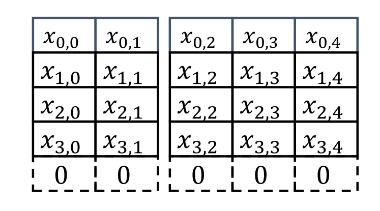
Figure 1: Diagram of the BR code with $p=5$ and $r=3$.

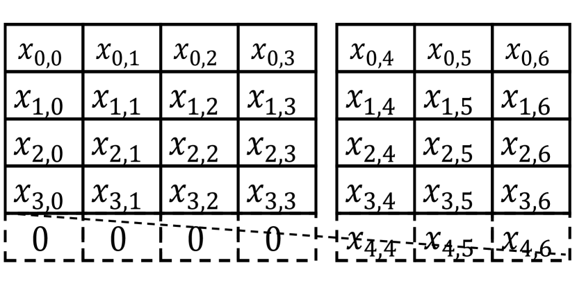
Figure 2: Diagram of the generalized RDP code with $p=5$ and $r=3$.

II-B IP codes

IP codes are also constructed in $\mathbb{R}_{p,1}$, but all parity columns are independent of each other, leading to a minimization of the number of parity updates when a data bit is updated [16, 2, 10]. Precisely, given the prime number $p$ and a positive integer $r$, the IP$(p+r,r)$ is defined as the set of $(p-1)\times(p+r)$ arrays of bits. In the same way as the BR codes, each column of the array forms a binary polynomial, then the parity-check matrix of the IP$(p+r,r)$ is $H_{IP}=\left(H_{BR}|I_{r}\right),$ where $H_{BR}$ is shown in (4) and $I_{r}$ is an $r\times r$ identity matrix. The matrix $H_{IP}$ implies that IP codes also have an intuitive graphical representation similar to that shown in BR codes. Contrary to BR codes, IP codes are not always binary MDS array codes. The conditions for making IP codes to be MDS array codes can be found in [2, 7].

II-C Generalized RDP codes

In [17], the authors presented a binary MDS array code with two parity columns, i.e., RDP codes. This code was generalized to support more parity columns in [1]. Generalized RDP codes are not directly constructed by parity-check matrices over $\mathbb{R}_{p,1}$ like the two codes introduced above. Given a prime number $p$ and a positive integer $r$, the generalized RDP$(p+r-1,r)$ code is defined as the set of $(p-1)\times(p+r-1)$ arrays (denoted by $[x_{i,j}]$, where $x_{i,j}\in\{0,1\}$, the first $p-1$ data columns are information columns, and others are parity columns). From [1], it satisfies the following encoding equations:

$$x_{i,p-1}=\sum_{j=0}^{p-2}x_{i,j}~{}\text{for}~{}0\leq i\leq p-2,$$ (5)

and $$x_{i,p-1+j}=\sum_{\ell=0}^{p-1}x_{i-j\ell,\ell}~{}\text{for}~{}{0\leq i\leq p-2,\atop 1\leq j\leq r-1},$$ (6)

where addition is performed through XOR, all subscripts in the right-hand side of equal signs are modulo $p$, and $x_{p-1,j}=0$ for $j=0,1,\cdots,p-1$.

Similar to BR and IP codes, the generalized RDP codes have an intuitive graphical representation. Figure 2 shows an example of $p=5$ and $r=3$, where the leftmost four data columns are information columns and the last row is imaginary. Clearly, the first parity column, i.e., $\{x_{i,4}\}_{i=0}^{4}$, is obtained by bit-wise XORing the first 4 columns. The second parity column, i.e., $\{x_{i,5}\}_{i=0}^{4}$, is obtained by bit-wise XORing the first 5 columns after each column has been subjected to down-cyclic shifts according to the corresponding column index size. The third parity column is similar to the second, but the number of down-cyclic shifts in each column becomes twice the corresponding column index size. The three parity columns of the generalized RDP$(7,3)$ code are obtained by directly deleting the imaginary row.

Generalized RDP codes are not always binary MDS array codes [1], as are IP codes. Conditions that make generalized RDP codes to be binary MDS array codes can be found in [1]. In particular, there is a connection between generalized RDP and shortened IP codes as follows [1]:

Theorem 1.

([1]) The generalized RDP$(p+r-1,r)$ is a binary MDS array code if the shortened IP$(p+r-1,r)$ with the following parity-check matrix over $\mathbb{R}_{p,1}$ is a binary MDS array code

$$H_{SIP}=\left(H_{BR}\quad\begin{array}[]{|cccccc}0&0&\cdots&0\\ 1&0&\cdots&0\\ 0&1&\cdots&0\\ \vdots&\vdots&\ddots&\vdots\\ 0&0&\cdots&1\end{array}\right).$$ (7)

The encoding of the shortened IP code with (7) can be analogized from the BR code in Section II-A. It is easy to see that the process is similar to that in the generalized RDP$(p+r-1,r)$. The only difference is that the latter does not need to calculate the last bit in each parity column and modulo $f_{p,1}(x)$.

II-D Notations

Throughout this paper, the set $\{0,1,2,3,\cdots\}$ is denoted by $\mathbb{N}$ and the set $\{i,i+1,\cdots,j-1\}$ is denoted by $[i,j)$, where $i\in\mathbb{N},j\in\mathbb{N}$ with $i<j$. The transpose of a matrix or vector is marked with the notation $\mathrm{T}$ in the upper right-hand corner. Unless otherwise stated, suppose that

$$m=p\tau,\qquad\tau=2^{s},$$ (8)

where $p>1$ is an odd number and $s\in\mathbb{N}$. Note that $p$ and $\tau$ are determined if $m$ is given. In addition, $f_{p,\tau}(x)=f_{p,1}^{\tau}(x)$.

Some special mappings are defined below. For any $i\in\mathbb{N},j\in\mathbb{N}$ and $a=\sum_{i=0}^{m-1}a_{i}\cdot x^{i}\in\mathbb{R}$, define a mapping $\mathcal{A}_{i,j}:\mathbb{R}\rightarrow\mathbb{F}_{2}^{(m-i)\times(m-j)}$ by letting $\mathcal{A}_{i,j}(a)$ be the resultant $(m-i)\times(m-j)$ binary matrix after deleting the last $i$ rows and last $j$ columns of the following $m\times m$ binary circulant matrix

$$\left(\begin{array}[]{ccccc}a_{0}&a_{1}&a_{2}&\cdots&a_{m-1}\\ a_{m-1}&a_{0}&a_{1}&\cdots&a_{m-2}\\ \vdots&\vdots&\vdots&\ddots&\vdots\\ a_{1}&a_{2}&a_{3}&\cdots&a_{0}\end{array}\right).$$ (9)

From [26], one can see that $\mathcal{A}_{0,0}$ is an isomorphic mapping. Moreover, for $i\in\mathbb{N}$, $\mathcal{A}_{i,i}(0)$ is the $(m-i)\times(m-i)$ zero matrix and $\mathcal{A}_{i,i}(1)$ is an $(m-i)\times(m-i)$ identity matrix. For any $\ell_{0}\in\mathbb{N}$ and $\ell_{1}\in\mathbb{N}$, we define a mapping from the set consisting of all $\ell_{0}\times\ell_{1}$ matrices over $\mathbb{R}$ to the set consisting of all $\ell_{0}(m-\tau)\times\ell_{1}(m-\tau)$ matrices over $\mathbb{F}_{2}$, i.e.,

$$\mathcal{T}_{\ell_{0},\ell_{1},m}:M_{\ell_{0}\times\ell_{1}}(\mathbb{R})\rightarrow M_{\ell_{0}(m-\tau)\times\ell_{1}(m-\tau)}(\mathbb{F}_{2})$$ (10)

by letting $\mathcal{T}_{\ell_{0},\ell_{1},m}(B)=\overline{B}$, where $B=[b_{i,j}]\in\mathbb{R}^{\ell_{0}\times\ell_{1}}$ and $\overline{B}=[\mathcal{A}_{\tau,\tau}(b_{i,j})]\in\mathbb{F}_{2}^{\ell_{0}(m-\tau)\times\ell_{1}(m-\tau)}$.

In this paper, the code with $\mathcal{T}_{\ell_{0},\ell_{1},m}(B)$ as the parity-check matrix has a binary codeword of size $\ell_{1}\cdot(m-\tau)$, where $\ell_{0}<\ell_{1}$. By default, the codeword is arranged in an $(m-\tau)\times\ell_{1}$ array of bits in column-first order, and we refer to this code as a binary array code. Also, we refer to this code as a binary MDS array code if each codeword can be restored by any $\ell_{1}-\ell_{0}$ columns.

III Definitions of Variant codes

This section defines two new classes of binary array codes (i.e., V-ETBR and V-ESIP codes), which both are variants of codes over the polynomial ring $\mathbb{R}_{p,\tau}$. All variant codes are based on binary parity-check matrices. One can see that the generalized RDP codes in Section II-C are a special case of the V-ESIP codes.

To begin with, we define two codes over the polynomial ring $\mathbb{R}_{p,\tau}$ as follows:

Definition 1.

(ETBR Codes) Let $2\leq r<n$, and $H=[h_{i,j}]_{0\leq i<r,0\leq j<n}\in\mathbb{R}^{r\times n}$. Define ETBR$(n,r,m=p\tau,H)$ as a code over $\mathbb{R}_{p,\tau}$ determined by the parity-check matrix $H$ that is reduced to over $\mathbb{R}_{p,\tau}$, where each element in $H$ over $\mathbb{R}$ is modulo $f_{p,\tau}(x)$ to be an element over $\mathbb{R}_{p,\tau}$.

Remark 1.

In Definition 1, the form of $H$ is not fixed and covers $H_{BR}$ in (4), so we refer to ETBR$(n,r,m,H)$ as an extended BR code.

Definition 2.

(ESIP Codes) Let $n\geq 2,r\geq 2$, and $H^{\prime}=[H|\widehat{I}]\in\mathbb{R}^{r\times(n+r-1)}$, where the definition of $H$ is the same as in Definition 1 and $\widehat{I}$ is the matrix after removing the first column of the $r\times r$ identity matrix. Define ESIP$(n,r,m=p\tau,H^{\prime})$ as a code over $\mathbb{R}_{p,\tau}$ determined by the parity-check matrix $H^{\prime}$ that is reduced to over $\mathbb{R}_{p,\tau}$, where each element in $H$ over $\mathbb{R}$ is modulo $f_{p,\tau}(x)$ to be an element over $\mathbb{R}_{p,\tau}$.

Remark 2.

In Definition 2, the ESIP$(n,r,m=p,H^{\prime})$ is exactly the shortened IP code given by (7) if $H=H_{BR}$. Obviously, $H^{\prime}$ has a wider range of parameters so that the ESIP codes can be regarded as an extension of shortened IP codes.

The variant codes corresponding to ETBR and ESIP codes, i.e., V-ETBR and V-ESIP codes, are defined below. When we refer to ETBR/ESIP codes and V-ETBR/V-ESIP codes as corresponding, it means that they are determined by the same matrix $H$ or $H^{\prime}$ over $\mathbb{R}$.

Definition 3.

(V-ETBR Codes) Define V-ETBR$(n,r,m=p\tau,H)$ as a binary array code whose parity-check matrix is $\mathcal{T}_{r,n,m}(H)$, where $2\leq r<n$, $\mathcal{T}_{r,n,m}$ is defined in (10), and the definition of $H$ is the same as that in Definition 1.

Definition 4.

(V-ESIP Codes) Define V-ESIP$(n,r,m=p\tau,H^{\prime})$ as a binary array code whose parity-check matrix is $\mathcal{T}_{r,n+r-1,m}(H^{\prime})$, where $n\geq 2,r\geq 2$, $\mathcal{T}_{r,n+r-1,m}$ is defined in (10), and the definition of $H^{\prime}$ is the same as that in Definition 2.

Conventionally, the last $r$ columns of the array corresponding to the codeword in the above codes are referred to as parity columns and all other columns are referred to as information columns. We have the following relationship.

Lemma 1.

Let $H^{\prime}$ in Definition 4 be determined by a Vandermonde matrix $H$ such that $h_{1,j}=x^{p-j}$ and $h_{i,j}=h_{1,j}^{i}$ for $2\leq i<r,0\leq j<p$, and $p$ is a prime number. Then V-ESIP$(p,r,m=p,H^{\prime})$ is exactly the generalized RDP$(p+r-1,r)$ described in Sec. II-C.

Proof.

From Definition 4, $\mathcal{T}_{r,p+r-1,p}(H^{\prime})$ is the parity-check matrix of the V-ESIP$(p,r,m=p,H^{\prime})$ and is given by (11) at the top of this page.

$$\mathcal{T}_{r,p+r-1,p}(H^{\prime})=\left(\begin{array}[]{cccccccc}I_{p-1}&I_{p-1}&I_{p-1}&\cdots&I_{p-1}&&&\\ I_{p-1}&\mathcal{A}_{1,1}(x^{p-1})&\mathcal{A}_{1,1}(x^{p-2})&\cdots&\mathcal{A}_{1,1}(x)&I_{p-1}&&\\ \vdots&\vdots&\vdots&\ddots&\vdots&&\ddots&\\ I_{p-1}&\mathcal{A}_{1,1}(x^{(p-1)(r-1)})&\mathcal{A}_{1,1}(x^{(p-2)(r-1)})&\cdots&\mathcal{A}_{1,1}(x^{r-1})&&&I_{p-1}\\ \end{array}\right).$$ (11)

Let $\mathbf{b}_{0},\mathbf{b}_{1},\cdots,\mathbf{b}_{p-2}\in\mathbb{F}_{2}^{p-1}$ denote all $p-1$ information columns in the codewrod. We next show that any parity column generated by the V-ESIP code is the same as that in the generalized RDP code described in Sec. II-C.

Let $\mathbf{b}_{p-1},\mathbf{b}_{p},\cdots,\mathbf{b}_{p+r-2}\in\mathbb{F}_{2}^{p-1}$ denote all $r$ parity columns of the V-ESIP code. One can easily know from (11) that $\mathbf{b}_{p-1}$ is obtained by bit-wise XORing all $p-1$ information columns. For any $i\in[1,r)$, the $i$-th parity column of the V-ESIP code is obtained by

$$\mathbf{b}_{p-1+i}^{\mathrm{T}}=\sum_{j=0}^{p-1}\mathcal{A}_{1,1}(x^{(p-j)i})\cdot\mathbf{b}_{j}^{\mathrm{T}}=\sum_{j=0}^{p-1}\mathcal{A}_{1,0}(x^{(p-j)i})\cdot(\mathbf{b}_{j},0)^{\mathrm{T}}.$$ (12)

We remark that calculating $\mathcal{A}_{1,0}(x^{(p-j)i})\cdot(\mathbf{b}_{j},0)^{\mathrm{T}}$ is equivalent to removing the last element from the result of $\mathcal{A}_{0,0}(x^{(p-j)i})\cdot(\mathbf{b},0)^{\mathrm{T}}$. Furthermore, $\mathcal{A}_{0,0}(x^{p-j})$ can be regarded as the operator of performing $j$ times down-cyclic shift on a vector and $\mathcal{A}_{0,0}(x^{(p-j)i})=\left(\mathcal{A}_{0,0}(x^{p-j})\right)^{i}$. Assume that each data column has an imaginary bit attached at the end, thus, (12) indicates that each $\mathbf{b}_{p-1+i},i\in[1,r)$ can be obtained by bit-wise XORing the first $p$ columns after each column has been subjected to down-cyclic shifts according to $i$ times the corresponding column index size. Each parity column needs to remove the last bit in the result. The above is consistent with the graphical representation of the generalized RDP code, as shown in Fig. 2. This completes the proof. ∎

Lemma 1 explicitly provides a binary parity-check matrix for the generalized RDP$(p+r-1,r)$, which was not given in other literature. From the perspective of the binary parity-check matrix, all fast computations about the generalized RDP codes, such as those proposed in [21, 27], can be regarded as scheduling schemes for matrix operations over binary fields. Furthermore, any existing scheduling algorithm for general matrix operations over binary fields can be used to accelerate the computation of generalized RDP codes.

Recall that Theorem 1 established a connection between generalized RDP codes and shortened IP codes, which can be viewed as a special case of the connection between V-ESIP codes and ESIP codes. It remains an open problem whether there exists a general connection between V-ESIP and ESIP codes, as well as between V-ETBR and ETBR codes. The next section is devoted to these issues.

IV Connections & explicit constructions

This section presents the general connections between the variant codes defined above and their corresponding codes over polynomial rings. Some explicit constructions for the V-ETBR/V-ESIP MDS array codes are then proposed.

IV-A General connections

This subsection starts by exploring the conditions of V-ETBR/V-ESIP codes to be binary MDS array codes. We first analyze the rank of the square matrix $\mathcal{T}_{\ell,\ell,m}(V)$. The following lemma is useful.

Lemma 2.

Assume that $\ell_{0}\geq 2,\ell_{1}\geq 2$, $x^{\tau}+1|a_{i,j}+a_{i,k}$ with $a_{i,j},a_{i,k}\in\mathbb{R},i\in[0,\ell_{0}),j,k\in[0,\ell_{1})$. Let each $\mathbf{a}_{i,j}$ denote the binary coefficient vector of $a_{i,j}$, i.e., $a_{i,j}=\mathbf{a}_{i,j}\cdot(1,x,\cdots,x^{m-1})^{\mathrm{T}}$, and let $\overline{\mathbf{a}}_{i,j}$ denote the vector after $\mathbf{a}_{i,j}$ deletes the last $\tau$ elements. If all vectors in the set $\{\left(\overline{\mathbf{a}}_{i,0},\cdots,\overline{\mathbf{a}}_{i,\ell_{1}-1}\right)\in\mathbb{F}_{2}^{1\times(m-\tau)\ell_{1}}\}_{i=0}^{\ell_{0}-1}$ are $\mathbb{F}_{2}$-linearly dependent, i.e., $\sum_{i=0}^{\ell_{0}-1}c_{i}\cdot\left(\overline{\mathbf{a}}_{i,0},\cdots,\overline{\mathbf{a}}_{i,\ell_{1}-1}\right)=\mathbf{0}_{1\times(m-\tau)\ell_{1}}$, where each $c_{i}\in\mathbb{F}_{2}$ and $c_{0},c_{1},\cdots,c_{\ell_{0}-1}$ are not all zero, then the result of $\sum_{i=0}^{\ell_{0}-1}c_{i}\cdot\left({\mathbf{a}}_{i,0},\cdots,{\mathbf{a}}_{i,\ell_{1}-1}\right)$ must have the form of $(\mathbf{0}_{1\times(m-\tau)},\mathbf{u}|\mathbf{0}_{1\times(m-\tau)},\mathbf{u},|\cdots|\mathbf{0}_{1\times(m-\tau)},\mathbf{u}),$ where $\mathbf{u}\in\mathbb{F}_{2}^{1\times\tau}$.

Proof.

From the condition, we immediately have

$$\sum_{i=0}^{\ell_{0}-1}c_{i}\cdot\left({\mathbf{a}}_{i,0},\cdots,{\mathbf{a}}_{i,\ell_{1}-1}\right)$$ (13)

$$= (\mathbf{0}_{1\times(m-\tau)},\mathbf{u}_{0}|\mathbf{0}_{1\times(m-\tau)},\mathbf{u}_{1},|\cdots|\mathbf{0}_{1\times(m-\tau)},\mathbf{u}_{\ell_{1}-1})$$

where each $\mathbf{u}_{i}\in\mathbb{F}_{2}^{1\times\tau}$. In the above formula, the sum of any two parts is $(\mathbf{0}_{1\times(m-\tau)},\mathbf{u}_{j}+\mathbf{u}_{k})=\sum_{i=0}^{\ell_{0}-1}c_{i}\cdot(\mathbf{a}_{i,j}+\mathbf{a}_{i,k})$, where $0\leq j<k<\ell_{1}$. Since $x^{\tau}+1|a_{i,j}+a_{i,k}$, then the sum $(\mathbf{0}_{1\times(m-\tau)},\mathbf{u}_{j}+\mathbf{u}_{k})$ is a binary coefficient vector of the polynomial that is a multiple of $x^{\tau}+1$. However, $\mathbf{u}_{j}+\mathbf{u}_{k}$ contains only $\tau$ elements. This results in $\mathbf{u}_{j}+\mathbf{u}_{k}$ having to be zero vector. Therefore, we have $\mathbf{u}_{j}=\mathbf{u}_{k}$ with $j\neq k$. This completes the proof. ∎

Remark 3.

From the proof of Lemma 2, one can readily know that $\mathbf{u}=\mathbf{0}_{1\times\tau}$ in Lemma 2, if $x+1|a_{i,j},i\in[0,\ell_{0}),j\in[0,\ell_{1})$.

TABLE I defines some important symbols to be used later. The following lemmas hold.

TABLE I: Important symbols used in Section IV

Symbol	Definition
$\ell$	a positive number not less than two.
$V$	$V=[v_{i,j}]$ is an $\ell\times\ell$ square matrix over $\mathbb{R}$.
$\mathcal{B}(i,j)$	$\mathcal{B}(i,j)=\left(\mathcal{A}_{\tau,0}(v_{i,0}),\cdots,\mathcal{A}_{\tau,0}(v_{i,j-1})\right)$, $i\in[0,\ell),j\in[1,\ell+1)$.
$\mathcal{B}_{\tau}(i,j)$	$\mathcal{B}_{\tau}(i,j)=\left(\mathcal{A}_{\tau,\tau}(v_{i,0}),\cdots,\mathcal{A}_{\tau,\tau}(v_{i,j-1})\right)$, $i\in[0,\ell),j\in[1,\ell+1)$.
$\overline{\mathbf{v}}_{i,j}$	a non-zero codeword with vector form that generated by generator matrix $\mathcal{B}_{\tau}(i,j)$.
${\mathbf{v}}_{i,j}$	the non-zero codeword with vector form that generated by generator matrix $\mathcal{B}(i,j)$ and corresponds to $\overline{\mathbf{v}}_{i,j}$.

Lemma 3.

The square matrix $\mathcal{T}_{\ell,\ell,m}(V)$ has full rank if the following conditions are satisfied:

1. $V$ has full rank over $\mathbb{R}_{p,\tau}$, i.e., $\gcd(|V|,f_{p,\tau}(x))=1$, where $|V|$ is the determinant of $V$.

2. For any $0\leq i<\ell$, then $\mathcal{B}_{\tau}(i,\ell)$ in TABLE I has full row rank over $\mathbb{F}_{2}$.

3. For any $0\leq i<\ell,0\leq j<\ell$, then $x^{\tau}+1|v_{i,j}$.

When $v_{0,j}=1,\forall j\in[0,\ell)$, 3) is relaxed to

1. For any $1\leq i<\ell,0\leq j<k<\ell$, then $x^{\tau}+1|v_{i,j}+v_{i,k}$.

Proof.

According to TABLE I, $\mathcal{T}_{\ell,\ell,m}(V)$ is composed of $\mathcal{B}_{\tau}(0,\ell),\mathcal{B}_{\tau}(1,\ell),\cdots,\mathcal{B}_{\tau}(\ell-1,\ell)$. Since each $\mathcal{B}_{\tau}(i,\ell),i\in[0,\ell)$, has full row rank, we only need to prove that there are no $\overline{\mathbf{v}}_{0,\ell},\overline{\mathbf{v}}_{1,\ell},\cdots,\overline{\mathbf{v}}_{\ell-1,\ell}$, which are $\mathbb{F}_{2}$-linearly dependent. By contradiction, assume that there exists $\overline{\mathbf{v}}_{0,\ell},\overline{\mathbf{v}}_{1,\ell},\cdots,\overline{\mathbf{v}}_{\ell-1,\ell}$ such that they are $\mathbb{F}_{2}$-linearly dependent, i.e., $\sum_{i=0}^{\ell-1}c_{i}\overline{\mathbf{v}}_{i,\ell}=\mathbf{0}_{1\times(m-\tau)\ell}$ where each $c_{i}\in\mathbb{F}_{2}$ and $c_{0},c_{1},\cdots,c_{\ell-1}$ are not all zero.

We first consider the third condition of $x^{\tau}+1|v_{i,j}$. According to Remark 3 and the facts that $x^{\tau}+1|v_{i,j}$, each ${\mathbf{v}}_{i,\ell}$ is the vector consisting of the binary coefficient vectors in $q_{i,\ell}\cdot(v_{i,0},v_{i,1},\cdots,v_{i,\ell-1})$, where $q_{i,\ell}\in\mathbb{R}\setminus\{0\}$ and $\deg(q_{i,\ell})<m-\tau$. then $\sum_{i=0}^{\ell-1}c_{i}{\mathbf{v}}_{i,\ell}=(\mathbf{0}_{1\times m},\cdots,\mathbf{0}_{1\times m})$ Therefore, we have $\sum_{i=0}^{\ell-1}c_{i}q_{i,\ell}\cdot v_{i,j}=0\mod x^{m}+1$ for $j\in[0,\ell)$. By taking $j=0,1,\cdots,\ell-1$, the above equations can be converted into

$$\Gamma_{0}\cdot\begin{pmatrix}c_{0}\cdot q_{0,\ell}\\ c_{1}\cdot q_{1,\ell}\\ \vdots\\ c_{\ell-1}\cdot q_{\ell-1,\ell}\end{pmatrix}=\mathbf{0}^{\mathrm{T}},$$ (14)

where $\mathbf{0}$ is a zero-row vector and

$$\Gamma_{0}=\left(\begin{array}[]{cccc}v_{0,0}&v_{1,0}&\cdots&v_{\ell-1,0}\\ v_{0,1}&v_{1,1}&\cdots&v_{\ell-1,1}\\ \vdots&\vdots&\ddots&\vdots\\ v_{0,\ell-1}&v_{1,\ell-1}&\cdots&v_{\ell-1,\ell-1}\end{array}\right).$$ (15)

In (14), all operations are performed in $\mathbb{R}$. Note that each $c_{i}\in\mathbb{F}_{2}$ and $\deg(q_{i,\ell})<m-\tau$, we can solve the above linear equations in $\mathbb{R}_{p,\tau}$. Since $|\Gamma_{0}|=|V|$ is invertible over $\mathbb{R}_{p,\tau}$, then $c_{0}q_{0,\ell}\cdots,c_{\ell-1}q_{\ell-1,\ell}$ in (14) must all be zero according to Cramer’s rule. Moreover, each $q_{i,\ell}\neq 0$ with $\deg(q_{i,\ell})<m-\tau$, so that $c_{0}=c_{1}=\cdots=c_{\ell-1}=0$. This contradicts the assumption at the beginning.

Consider the third condition of $x^{\tau}+1|v_{i,j}+v_{i,k}$ instead, then Lemma 3 gives $\sum_{i=0}^{\ell-1}c_{i}{\mathbf{v}}_{i,\ell}=(\mathbf{0}_{1\times(m-\tau)},\mathbf{u}|\cdots|\mathbf{0}_{1\times(m-\tau)},\mathbf{u})$, where $\mathbf{u}\in\mathbb{F}_{2}^{m-\tau}$. Since $v_{0,j}=1,\forall j\in[0,\ell)$, we have

$$\sum_{i=1}^{\ell-1}c_{i}{\mathbf{v}}_{i,\ell}$$ (16)

$$= c_{0}\cdot\mathbf{v}_{0,\ell}+(\mathbf{0}_{1\times(m-\tau)},\mathbf{u}|\cdots|\mathbf{0}_{1\times(m-\tau)},\mathbf{u})=(\mathbf{u}^{\prime}|\cdots|\mathbf{u}^{\prime}),$$

where $\mathbf{u}^{\prime}\in\mathbb{F}_{2}^{m}$. Based on the fact that any two part of the form in (16) sum to zero, we have $\sum_{i=1}^{\ell-1}c_{i}q_{i,\ell}\cdot(v_{i,j}+v_{i,k})=0\mod x^{m}+1$ for $0\leq j<k<\ell$. By taking $(j,k)=(0,1),(0,2),\cdots,(0,\ell-1)$, the above equations can be converted into

$$\Gamma_{1}\cdot\begin{pmatrix}c_{1}\cdot q_{1,\ell}\\ c_{2}\cdot q_{2,\ell}\\ \vdots\\ c_{\ell-1}\cdot q_{\ell-1,\ell}\end{pmatrix}=\mathbf{0}^{\mathrm{T}},$$ (17)

where $\mathbf{0}$ is a zero-row vector and

$$\Gamma_{1}=\begin{pmatrix}v_{1,0}+v_{1,1}&\cdots&v_{\ell-1,0}+v_{\ell-1,1}\\ v_{1,0}+v_{1,2}&\cdots&v_{\ell-1,0}+v_{\ell-1,2}\\ \vdots&\ddots&\vdots\\ v_{1,0}+v_{1,\ell-1}&\cdots&v_{\ell-1,0}+v_{\ell-1,\ell-1}\\ \end{pmatrix}.$$ (18)

In (17), all operations are performed in $\mathbb{R}$. Note that each $c_{i}\in\mathbb{F}_{2}$ and $\deg(q_{i,\ell})<m-\tau$, we next solve the above linear equations in $\mathbb{R}_{p,\tau}$. One can know that the determinant of $\Gamma_{1}$ is equal

$$\left|\begin{array}[]{cccc}1&0&\cdots&0\\ 1&v_{1,0}+v_{1,1}&\cdots&v_{\ell-1,0}+v_{\ell-1,1}\\ \vdots&\vdots&\ddots&\vdots\\ 1&v_{1,0}+v_{1,\ell-1}&\cdots&v_{\ell-1,0}+v_{\ell-1,\ell-1}\\ \end{array}\right|$$ (19)

$$= \left|\begin{array}[]{cccc}1&v_{1,0}&\cdots&v_{\ell-1,0}\\ 1&v_{1,1}&\cdots&v_{\ell-1,1}\\ \vdots&\vdots&\ddots&\vdots\\ 1&v_{1,\ell-1}&\cdots&v_{\ell-1,\ell-1}\end{array}\right|=|V|,$$

where the first equality is obtained by subtracting the appropriate multiple of the first column from all other columns. Thus, $|\Gamma_{1}|=|V|$ is also invertible over $\mathbb{R}_{p,\tau}$. Then $c_{1}q_{1,\ell}\cdots,c_{\ell-1}q_{\ell-1,\ell}$ in (14) must all be zero according to Cramer’s rule. Similarly, note that each $q_{i,\ell}\neq 0$ with $\deg(q_{i,\ell})<m-\tau$, so we must have that $c_{1}=\cdots=c_{\ell-1}=0$, then $c_{0}=0$. This contradicts the assumption at the beginning. This completes the proof. ∎

In Lemma 3, the latter two conditions are easily met. More precisely, the third condition only requires that any $v_{i,j}$ is a multiple of $x^{\tau}+1$, and the second condition can be satisfied by the following lemma, which is easily obtained through the proof of Proposition 6 in [25].

Lemma 4.

([25]) If $\gcd(a,x^{m}+1)=x^{\tau}+1$ or $\gcd(a+b,x^{m}+1)=x^{\tau}+1$, where $a,b\in\mathbb{R}$, then $\mathcal{A}_{\tau}(a,b)$ has full row rank over $\mathbb{F}_{2}$.

We now present the connection between V-ETBR/V-ESIP codes and ETBR/ESIP codes.

Corollary 1.

(Connection) V-ETBR$(n,r,m=p\tau,H)$ is a binary MDS array code if

1. The corresponding ETBR$(n,r,m,H)$ is an MDS code over $\mathbb{R}_{p,\tau}$.

2. For any $0\leq i<r,0\leq j<n$, then $\gcd(h_{i,j},x^{m}+1)=x^{\tau}+1$.

When $h_{0,j}=1,\forall j\in[0,n)$, the above last condition is replaced with

1. For any $1\leq i<r,0\leq j,k<n$ and $j\neq k$, then $\gcd(v_{i,j},x^{m}+1)=x^{\tau}+1$ or $\gcd(v_{i,j}+v_{i,k},x^{m}+1)=x^{\tau}+1$.

Proof.

We only need to prove that any $\mathcal{T}_{\ell\times\ell}(V)$ for $\ell=r$ has full rank, where all elements in $V$ are determined by $H$. This is easily derived from Lemma 3 and 4.

∎

Corollary 2.

(Connection) When the first row of $H$ in $H^{\prime}$ is an all-one row, the V-ESIP$(n,r,m=p\tau,H^{\prime})$ is a binary MDS array code if

1. The corresponding ESIP$(n,r,m,H^{\prime})$ is an MDS code over $\mathbb{R}_{p,\tau}$.

2. For any $1\leq i<r$ and $0\leq j<k<n$, then $x^{\tau}+1|h_{i,j}+h_{i,k}$.

Proof.

Without loss of generality, we only need to prove $\mathcal{T}_{\ell,\ell,m}(V)$ for any $1<\ell\leq r$ has full rank, where elements in $\mathcal{T}_{\ell,\ell,m}(V)$ are determined by $H^{\prime}$ and $\{v_{0,j}=1\}_{j=0}^{\ell-1}$. We prove this via Lemma 3. First, the first condition of Lemma 3 is satisfied since the corresponding ESIP$(n,r,m,H^{\prime})$ is an MDS code over $\mathbb{R}$. Furthermore, the fact that $V$ with $\ell=2$ have full rank over $\mathbb{R}_{p,\tau}$ leads to $\gcd(h_{i,j}+h_{i,k},f_{p,\tau}(x))=1,1\leq i<r,0\leq j<k<n$. Recall that the condition of $x^{\tau}+1|h_{i,j}+h_{i,k}$, then we have $\gcd(h_{i,j}+h_{i,k},x^{m}+1)=x^{\tau}+1$. One can easily see from Lemma 4 that the second condition of Lemma 3 is thus satisfied. The latter third condition of Lemma 3 is obviously satisfied. This completes the proof. ∎

Remark 4.

Now, the correctness of Theorem 1 can be readily proven by Corollary 2, just by setting $\tau=1$. Theorem 1 requires $p$ to be an odd prime number for shortened IP codes. Corollary 2 provides additional clarification by demonstrating that $p$ only needs to be odd.

In Corollary 2, the rightmost end of $H^{\prime}$ is not necessarily an identity matrix. Since the existence of an identity matrix can simplify encoding, we consider the following case. Note that the following case does not require the first row of $H$ to be an all-one row, only the last column to be constrained.

Corollary 3.

(Connection) Assuming the rightmost end of $H^{\prime}$ is an $r\times r$ identity matrix, i.e., the last column of $H$ is $(1,0,0,\cdots,0)^{\mathrm{T}}$, then the V-ESIP$(n,r,m=p\tau,H^{\prime})$ is a binary MDS array code if

1. The corresponding ESIP$(n,r,m,H^{\prime})$ is an MDS code over $\mathbb{R}_{p,\tau}$.

2. For any $0\leq i<r$ and $0\leq j<n-1$, then $\gcd(h_{i,j},x^{m}+1)=x^{\tau}+1$.

Proof.

Without loss of generality, we only need to prove $\mathcal{T}_{\ell,\ell,m}(V)$ for any $1\leq\ell\leq r$ has full rank, where elements in $\mathcal{T}_{\ell,\ell,m}(V)$ are determined by $H$ after removing the last column. Similarly, we prove this via Lemma 3. First, the first condition of Lemma 3 is satisfied since the corresponding ESIP$(n,r,m,H^{\prime})$ is an MDS code over $\mathbb{R}$. Lemma 4 and $\gcd(h_{i,j},x^{m}+1)=x^{\tau}+1$ leads to that the second condition of Lemma 3 holds. Finally, the former third condition of Lemma 3 obviously holds. This completes the proof. ∎

IV-B Explicit constructions

We next present some explicit constructions for the V-ETBR/V-ESIP MDS array codes. To begin with, suppose that $f_{p,1}(x)$ in (2) can be completely factorized into $f_{p,1}(x)=f_{0}(x)\cdot f_{1}(x)\cdots f_{\mu-1}(x),$ where each $f_{i}(x)$ is irreducible polynomial over $\mathbb{F}_{2}[x]$ and $\lambda=deg(f_{0}(x))\leq deg(f_{1}(x))\leq\cdots\leq deg(f_{\mu-1}(x))$. Note that $\lambda=p-1$ if $2$ is a primitive element in $p$-ary finite field $\mathbb{F}_{p}$ [2]. Then we have the following construction for the V-ESIP MDS array codes with any number of parity numbers, based on Cauchy matrices.

Construction 1.

(V-ESIP MDS array codes with $r\geq 2$) Let $\{a_{0},\cdots,a_{r-1}\}$ and $\{b_{0},\cdots,b_{n-2}\}$ are two sets of elements from $\mathbb{R}$, where $\deg(a_{i})<\lambda,\deg(b_{j})<\lambda$ and $a_{i}\neq b_{j}$ for any $i,j$, then the V-ESIP$(n,r\geq 2,m=p\tau,H^{\prime}=[H_{I}|I_{r\times r}])$ is a binary MDS array code, where $H_{I}=[({x^{\tau}+1})\cdot g_{i}]\in\mathbb{R}^{r\times(n-1)}$ and $g_{i}$ denotes the inverse of ${a_{i}+b_{j}}$ over $\mathbb{R}_{p,\tau}$ that always exists due to the degree of ${a_{i}+b_{j}}$ less than $\lambda$.

Proof.

We prove this via Corollary 3. Let $H_{I}^{\prime}=[g_{i}=\frac{1}{a_{i}+b_{j}}]\in\mathbb{R}_{p,\tau}^{r\times(n-1)}$ be a Cauchy matrix. Obviously, the determinant of any square sub-matrix of $H_{I}^{\prime}$ is invertible over $\mathbb{R}_{p,\tau}$, since it is the product of some elements in the sets $\{a_{i}+a_{j}\}_{i\neq j},\{b_{i}+b_{j}\}_{i\neq j},\{\frac{1}{a_{i}+b_{j}}\}$ [28], where any $a_{i},b_{j}$ has the degree less than $\lambda$. Note that the determinant of the corresponding square sub-matrix of $H_{I}$ is $x^{\tau}+1$ times the above result, and $\gcd(x^{\tau}+1,f_{p,\tau}(x))=1$. This results in the determinant of any square sub-matrix of $H_{I}$ having to be invertible over $\mathbb{R}_{p,\tau}$. Thus, the first condition of Corollary 3 is satisfied. Furthermore, we have $\gcd({(x^{\tau}+1)}g_{i},f_{p,\tau}(x))=1$, leading to the second condition of Corollary 3 holds. This completes the proof. ∎

Based on Vandermonde matrices, the following provides the construction of the V-ETBR MDS array codes with any number of parity columns. Note that this construction can also be found in [25]. For completeness, a different proof is provided based on the connection between V-ETBR and ETBR codes in Corollary 1. From the proof of any construction proposed in this paper, one can see that the codes over $\mathbb{R}_{p,\tau}$ corresponding to the variant codes are also MDS codes. In addition, [25] provided a fast scheduling scheme for the syndrome computation of the Vandermonde-based V-ETBR MDS array codes with $r\leq 3$. The next section of this paper will propose the generalization of this scheme suitable for any size of $r$.

To simplify the representation of elements in the Vandermonde matrix $H$, we let $h_{0,i}=1,\forall i\in[0,n),$ and $h_{i}:=h_{1,i},\forall i\in[0,n),$ such that $h_{j,i}=h_{i}^{j},\forall j\in[1,r),i\in[0,n)$.

Construction 2.

(V-ETBR MDS array codes with $r\geq 2$) Let $H\in\mathbb{R}^{r\times n}$ be a Vandermonde matrix, $n=2^{n_{0}},n_{0}\leq\lambda,$ and $h_{i}=(1+x^{\tau})\cdot h_{i}^{\prime},\forall i\in[0,n)$, where $\{h_{i}^{\prime}\}_{0\leq i<n}$ is given by $h_{0}^{\prime}=0$ and $h_{i+2^{j}}^{\prime}=h_{i}^{\prime}+x^{j},{0\leq j<n_{0},0\leq i<2^{j}}.$ Then the V-ETBR$(n,2\leq r<n,m=p\tau,H)$ is a binary MDS array code.

Proof.

We prove this via Corollary 1. Since the degree of any $h_{i}^{\prime}$ is less than $\lambda$, we have $gcd(h_{i}^{j},x^{m}+1)=(x^{\tau}+1)\cdot gcd((h_{i}^{\prime})^{j},f_{p,1}^{\tau}(x))=x^{\tau}+1$, where $1\leq i<r$ and $0\leq j<k<n$. This results in that the latter second condition of Corollary 1 holds. For the first condition of Corollary 1, we have $gcd(h_{j}+h_{k},f_{p,\tau}(x))=gcd(h_{j}^{\prime}+h_{k}^{\prime},f_{p,1}^{\tau}(x))=1$, where $0\leq j<k<n$. Then any $r\times r$ Vandermonde sub-matrix of $H$ is invertible over $\mathbb{R}_{p,\tau}$, leading to the ETBR$(n,r,m=p\tau,H)$ being MDS code over $\mathbb{R}_{p,\tau}$. This completes the proof. ∎

According to Corollary 2, it is not difficult to check that the V-ESIP$(n,r=3,m=p\tau,H^{\prime})$ is also a binary MDS array code if $H^{\prime}$ is determined by $H$ in Construction 2. The code has a systematic parity-check matrix that contains a $3\times 3$ identity matrix and has been focused on in [25]. The following provides the Vandermonde matrix-based construction for the V-ESIP MDS array code with $r=4$.

Construction 3.

(V-ESIP MDS array codes with $r=4$) Let $H\in\mathbb{R}^{r\times n}$ be a Vandermonde matrix, $n=2^{n_{1}}+1,n_{1}\leq w=\lfloor\frac{\lambda-1}{2}\rfloor$, $h_{n-1}=0$, and $h_{i}=(h_{i}^{\prime}+x^{w})\cdot(1+x^{\tau})$, where $i\in[0,2^{n_{1}})$ and $\{h_{i}^{\prime}\}_{0\leq i<2^{n_{1}}}$ is given by $h_{0}^{\prime}=0,h_{i+2^{j}}^{\prime}=h_{i}^{\prime}+x^{j},{0\leq j<n_{1},0\leq i<2^{j}}.$ Then the V-ESIP$(n,r=4,m=p\tau,H^{\prime})$ is a systematic binary MDS array code.

Proof.

We prove this via Corollary 2. The second condition in Corollary 2 obviously holds. For the first condition in Corollary 2, we only need to prove that any $4\times 4$ sub-matrix of $H^{\prime}$ is invertible over $\mathbb{R}_{p,\tau}$. Specifically, we first consider any $4\times 4$ sub-matrix of $H$ in $H^{\prime}$, which is a Vandermonde square matrix. Clearly, for any $0\leq i<j<n-1$, we have that $gcd(h_{i}+h_{j},f_{p,\tau}(x))=gcd(h_{i}^{\prime}+h_{j}^{\prime},f_{p,\tau}^{\tau}(x))$ and $gcd(h_{i}+h_{n-1},f_{p,1}^{\tau}(x))=gcd(h_{i}^{\prime}+x^{w},f_{p,1}^{\tau}(x))$. Since each $deg(h_{i}^{\prime})<w<\lambda$, then $gcd(h_{i}+h_{j},f_{p,\tau}(x))=1,\forall 0\leq i<j<n$. This indicates that any $4\times 4$ sub-matrix of $H$ is invertible over $\mathbb{R}_{p,\tau}$. Next, we focus on the remaining cases. We only need to determine if the following matrices are invertible over $\mathbb{R}_{p,\tau}$,

$$\begin{pmatrix}1&1\\ h_{i}^{3}&h_{j}^{3}\end{pmatrix},\quad\begin{pmatrix}1&1&1\\ h_{i}&h_{j}&h_{k}\\ h_{i}^{3}&h_{j}^{3}&h_{k}^{3}\end{pmatrix},\quad\begin{pmatrix}1&1&1\\ h_{i}^{2}&h_{j}^{2}&h_{k}^{2}\\ h_{i}^{3}&h_{j}^{3}&h_{k}^{3}\end{pmatrix},$$ (20)

where $0\leq i<j<k<n$. According to generalized Vandermonde determinants [29], the determinants of the above three matrices are respectively (let $h_{n-1}^{\prime}=0$)

$$h_{i}^{3}+h_{j}^{3}=(h_{i}+h_{j})(1+x^{\tau})^{2}\cdot\left((h_{i}^{\prime})^{2}+h_{i}^{\prime}h_{j}^{\prime}+(h_{j}^{\prime})^{2}\right.$$ (21)

$$\qquad\qquad\left.+(h_{i}^{\prime}+h_{j}^{\prime})x^{w}+x^{2w}\right),$$

$$h_{i}+h_{j}+h_{k}=(1+x^{\tau})(h_{i}^{\prime}+h_{j}^{\prime}+h_{k}^{\prime}+x^{w}),$$

$$h_{i}h_{j}+h_{i}h_{k}+h_{j}h_{k}=(1+x^{\tau})^{2}$$

$$\qquad\qquad\cdot(h_{i}^{\prime}h_{j}^{\prime}+h_{i}^{\prime}h_{k}^{\prime}+h_{j}^{\prime}h_{k}^{\prime}+x^{2w}),$$

where $0\leq i<j<k<n$. Since all $h_{i}^{\prime},h_{j}^{\prime},h_{k}^{\prime}$ have degree less than $w$, the above three values are not zero. Furthermore, due to $2w<\lambda$, it is not difficult to see that they are all coprime with $f_{p,\tau}(x)$. Then all the matrices in (20) are invertible over $\mathbb{R}_{p,\tau}$. This completes the proof. ∎

Remark 5.

It is clear that all the codes in Construction 1, 2 and 3 allow the total number of data columns to reach the exponential size with respect to the design parameter $p$. This is suitable for the needs of large-scale storage systems [25]. In addition, it is possible to construct the new codes using other matrices, such as Moore matrices [30] and some matrices searched by computers. All proposed connections in Section IV-A offer great flexibility in constructing the variant codes.

V Fast Computations

This section presents fast computations for the V-ETBR MDS array codes in Construction 2 and the V-ESIP MDS array codes in Construction 3. One can know from coding theory that the product of any parity-check matrix and its corresponding codeword is zero [31]. Formally, $\mathbf{0}^{\mathrm{T}}=\widehat{H}\cdot\widehat{\mathbf{x}}^{\mathrm{T}}$, where $\mathbf{0}$ denotes a zero vector, $\widehat{H}$ denotes a binary parity-check matrix, and $\widehat{\mathbf{x}}$ denotes the corresponding codeword. It follows that $\widehat{H}\cdot\mathbf{x}^{\mathrm{T}}=\widehat{H}_{e}\cdot\mathbf{e}^{\mathrm{T}}$, where $\mathbf{x}$ denotes the codeword after all erased symbols are set to zero, $\mathbf{e}$ denotes the vector consisting of all erased symbols, and $\widehat{H}_{e}$ denotes the sub-matrix of $\widehat{H}$ corresponding to $\mathbf{e}$. The above leads to the following common framework for encoding and decoding procedures [32, 3]: (when encoding, all parity symbols can be regarded as erased symbols.)

1. Compute syndrome $\mathbf{s}^{\mathrm{T}}:=\widehat{H}\cdot\mathbf{x}^{\mathrm{T}}$.

2. Solve linear equations $\mathbf{s}^{\mathrm{T}}=\widehat{H}_{e}\cdot\mathbf{e}^{\mathrm{T}}$.

V-A For Construction 2

Here, $\widehat{H}=\mathcal{T}_{r,n,m}(H)$, then the syndrome computation is $\mathbf{s}^{\mathrm{T}}=\mathcal{T}_{r,n,m}(H)\cdot\mathbf{x}^{\mathrm{T}}$. Let $\mathbf{x}=(\mathbf{x}_{0},\cdots\mathbf{x}_{n-1})$ and $\mathbf{s}=(\mathbf{s}_{0},\cdots\mathbf{s}_{r-1})$ with each $\mathbf{x}_{i}\in\mathbb{F}_{2}^{m-\tau},\mathbf{s}_{i}\in\mathbb{F}_{2}^{m-\tau}$.

V-A1 Syndrome computation

For any $i\in[0,r)$, we have

$$\mathbf{s}_{i}^{\mathrm{T}}= \sum_{j=0}^{2^{n_{0}}-1}\mathcal{A}_{\tau,\tau}(h_{j}^{i})\cdot\mathbf{x}_{j}^{\mathrm{T}}$$ (22)

$$= \sum_{j=0}^{2^{n_{0}}-1}\mathcal{A}_{\tau,\tau}\left((h_{j}^{\prime})^{i}\cdot(1+x^{\tau})^{i}\right)\cdot\mathbf{x}_{j}^{\mathrm{T}}.$$

The following is dedicated to demonstrating that when $n_{0}$ approaches infinity, $\mathbf{s}$ can be calculated with the asymptotic complexity of $\lfloor\lg r\rfloor+1$ XORs per data bit.

We first focus on the auxiliary calculation, i.e., $(\mathbf{s}_{i}^{*})^{\mathrm{T}}=\sum_{j=0}^{2^{n_{0}}-1}\mathcal{A}_{0,0}\left((h_{j}^{\prime})^{i}\cdot(1+x^{\tau})^{i}\right)\cdot(\mathbf{x}_{j}^{*})^{\mathrm{T}},$ where $i\in[0,r)$, $\mathbf{s}_{i}^{*}\in\mathbb{F}_{2}^{m}$ and $\mathbf{x}_{i}^{*}=(\mathbf{x}_{i},{0,0,\cdots,0})\in\mathbb{F}_{2}^{m}$. Obviously, for any $i\in[0,r)$, the first $m-\tau$ symbols in $\mathbf{s}_{i}^{*}$ exactly form $\mathbf{s}_{i}$. Note that the auxiliary calculation can be converted into $(\mathbf{s}_{i}^{*})^{\mathrm{T}}=\mathcal{A}_{0,0}\left((1+x^{\tau})^{i}\right)\cdot\sum_{j=0}^{2^{n_{0}}-1}\mathcal{A}_{0,0}\left((h_{j}^{\prime})^{i}\right)\cdot(\mathbf{x}_{j}^{*})^{\mathrm{T}},$ since $\mathcal{A}_{0,0}$ is an isomorphic mapping. After that, we have

$$(\mathbf{s}_{i})^{\mathrm{T}}=\mathcal{A}_{\tau,0}\left((1+x^{\tau})^{i}\right)\cdot P(i,\{\mathbf{x}_{j}^{*}\}_{j=0}^{2^{n_{0}}-1}),$$ (23)

where $i\in[0,r)$ and

$$P(i,\{\mathbf{x}_{j}^{*}\}_{j=0}^{2^{n_{0}}-1}):=\sum_{j=0}^{2^{n_{0}}-1}\mathcal{A}_{0,0}\left((h_{j}^{\prime})^{i}\right)\cdot(\mathbf{x}_{j}^{*})^{\mathrm{T}}.$$ (24)

Formula (24) can be calculated via Lemma 5.

Lemma 5.

Let $\mathbf{y}^{\mathrm{T}}=(\mathbf{y}_{0},\mathbf{y}_{1},\cdots,\mathbf{y}_{2^{n_{0}}-1})^{\mathrm{T}}=(R_{n_{0}}\otimes I_{m})\cdot(\mathbf{x}_{0}^{*},\mathbf{x}_{1}^{*},\cdots,\mathbf{x}_{2^{n_{0}}-1}^{*})^{\mathrm{T}},$ where each $\mathbf{y}_{i}\in\mathbb{F}_{2}^{m},\mathbf{x}_{i}^{*}\in\mathbb{F}_{2}^{m}$, $\otimes$ denotes Kronecker product, $I_{m}$ denotes an $m\times m$ identity matrix, and $R_{n_{0}}$ is a Reed-Muller matrix defined by $R_{0}=(1)$ and $R_{i+1}=\begin{pmatrix}R_{i}&R_{i}\\ &R_{i}\end{pmatrix},\forall i\in\mathbb{N}.$ Then (24) can be quickly calculated via (25), which is given at the bottom of this page.

$$P(i,\{\mathbf{x}_{j}^{*}\}_{j=0}^{2^{n_{0}}-1})=\begin{cases}\mathbf{y}_{0}^{\mathrm{T}},&i=0,\\ \sum_{t=1}^{b(i)}\sum_{n_{0}>\ell_{0}>\ell_{1}>\cdots>\ell_{t-1}\geq 0}\mathcal{A}_{0,0}\left(\delta(i;t;\ell_{0},\ell_{1},\cdots,\ell_{t-1})\right)\cdot\mathbf{y}_{\sum_{\ell=0}^{t-1}2^{\ell_{\ell}}}^{\mathrm{T}},&\forall i\in[1,r).\end{cases}$$ (25)

In (25), $b(i)$ is the number of 1’s in the binary representation of $i$,

$$\delta(i;t;\ell_{0},\ell_{1},\cdots,\ell_{t-1})$$ (26)

$$= \begin{cases}x^{\ell_{0}i_{0}},&\text{if}~{}t=1,\\ \sum_{i_{1}\in C_{i_{0}}^{\prime},i_{2}\in C_{i_{1}}^{\prime},\atop\cdots,i_{t-1}\in C_{i_{t-2}}^{\prime}}x^{\ell_{0}i_{0}+\sum_{\xi=1}^{t-1}(\ell_{\xi}-\ell_{\xi-1})\cdot i_{\xi}},&\text{if}~{}t>1,\end{cases}$$

where $i_{0}=i$, $C_{i}$ is the set consisting of the positions of non-zero bits in the binary representation of $i$, i.e., $i=\sum_{j\in C_{i}}2^{j}$, and $C_{i}^{\prime}=\{j|0<j<i,C_{j}\subset C_{i}\}$.

Proof.

Please see Appendix VI for the details. ∎

From Lemma 5, the syndrome computation in (23) can be completed through the following steps (pre-processing: calculate all required parameters $\delta$ according to (26)):

1. Calculate $\{\mathbf{y}_{i}|i\in[0,2^{n_{0}}),b(i)\leq\lfloor\lg r\rfloor\}$ via the Reed-Muller transform with input $(\mathbf{x}_{0}^{*},\cdots,\mathbf{x}_{2^{n_{0}}-1}^{*})$ and transform matrix $R_{n_{0}}\otimes I_{m}$. Note that $\lfloor\lg r\rfloor=\max\{b(i)|i\in[1,r)\}$.

2. Calculate $\{P(i,\{\mathbf{x}_{j}^{*}\}_{j=0}^{2^{n_{0}}-1})\}_{i=0}^{r-1}$ according to (25).

3. Calculate $\{\mathbf{s}_{i}\}_{i=0}^{r-1}$ according to (23).

$$\sum_{j=0}^{2^{n_{1}}-1}\mathcal{A}_{0,0}\left((h_{j}^{\prime}+x^{w})^{i}\right)\cdot(\mathbf{x}_{j}^{*})^{\mathrm{T}}=\begin{cases}P(0,\{\mathbf{x}_{j}^{*}\}_{j=0}^{2^{n_{1}}-1}),&i=0,\\ P(i,\{\mathbf{x}_{j}^{*}\}_{j=0}^{2^{n_{1}}-1})+\mathcal{A}_{0,0}\left(x^{iw}\right)\cdot P(0,\{\mathbf{x}_{j}^{*}\}_{j=0}^{2^{n_{1}}-1}),&i=1,2,\\ {\begin{aligned} &P(3,\{\mathbf{x}_{j}^{*}\}_{j=0}^{2^{n_{1}}-1})+\mathcal{A}_{0,0}\left(x^{w}\right)\cdot P(2,\{\mathbf{x}_{j}^{*}\}_{j=0}^{2^{n_{1}}-1})\\ &+\mathcal{A}_{0,0}\left(x^{2w}\right)\cdot P(1,\{\mathbf{x}_{j}^{*}\}_{j=0}^{2^{n_{1}}-1})+\mathcal{A}_{0,0}\left(x^{3w}\right)\cdot P(0,\{\mathbf{x}_{j}^{*}\}_{j=0}^{2^{n_{1}}-1})\end{aligned}},&i=3.\end{cases}$$ (27)

In Step 2, the operation of multiplying $\mathcal{A}_{0,0}(\delta(\bullet))$ by a vector can be simplified when $r<8$ due to the fact that $\delta(\bullet)$ is the sum of at most two monomials in this case. Specifically, we have $\mathcal{A}_{0,0}(x^{i}+x^{j})=\mathcal{A}_{0,0}(x^{i})+\mathcal{A}_{0,0}(x^{j})$ for all $i,j\in\mathbb{N}$, and each $\mathcal{A}_{0,0}(x^{i})$ can be viewed as a cyclic-shift operator that shifts a vector by $i$ bits. Therefore, when $r<8$, the multiplication of $\mathcal{A}_{0,0}(\delta(\bullet))$ by a vector can be easily implemented using at most one vector addition and one circular shift. When $r\geq 8$, it is best to use matrix-vector multiplication for this operation. This is because $\delta(\bullet)$ contains many monomials that need to be summed, and there exist scheduling algorithms that can reduce the complexity of matrix-vector multiplications, such as those described in [23, 24]. In Step 3, we have $\mathcal{A}_{\tau,0}\left((1+x^{\tau})^{i}\right)=\mathcal{A}_{\tau,0}(1)\cdot\Pi_{j\in C_{i}}\mathcal{A}_{0,0}(1+x^{\tau 2^{j}})$, leading to Step 3 being completed in the same way as above.

V-A2 Complexity analysis

In the above process, Step 1 requires only a portion of the Reed-Muller transform, and one can know from [3] that it produces XORs with the number of $(m-\tau)\cdot\left((\lfloor\lg r\rfloor+1)n+\small{o}(n)\right)$ [3], where little-o notation is used to describe an upper bound that cannot be tight. Step 2 produces matrix-vector multiplications and vector additions that are both $\sum_{i=1}^{r-1}\sum_{t=1}^{b(i)}\binom{n_{0}}{t}-r+1$. When $r$ is a constant, it is not difficult to check that $\lim_{n_{0}\rightarrow\infty}\frac{\sum_{i=1}^{r-1}\sum_{t=1}^{b(i)}\binom{n_{0}}{t}}{2^{n_{0}}/n_{0}}=0$. Thus, the total number of XORs required for Step 2 is $m^{2}\cdot\small{o}(2^{n_{0}}/n_{0})$. Step 3 produces $r-1$ matrix-vector multiplications. In summary, when $r$ and $\tau$ are constants and $n=2^{n_{0}}$ approaches infinity, the asymptotic complexity of the above syndrome computation is dominated by Step 1, and requires $\lfloor\lg r\rfloor+1$ XORs per data bit. Note that $m=p\tau$ and $p=\Theta(n_{0})$, where big-$\Theta$ notation is used to describe a bound within a constant factor. For visualization, TABLE II lists the total computational complexities required for the proposed syndrome computation with different parameters. It can be observed that the numerical results are close to the theoretical ones, especially when $n_{0}$ is large enough. Indeed, the syndrome computation proposed in [25], which reaches an asymptotic complexity of two XORs per data bit, is a special case of the above scheme at $r=3$.

V-B For Construction 3

Here, let $\mathbf{x}=(\mathbf{x}_{0},\cdots\mathbf{x}_{n+3})$ of each $\mathbf{x}_{i}\in\mathbb{F}_{2}^{m-\tau}$ be a codeword, and $\mathbf{s}=(\mathbf{s}_{0},\cdots\mathbf{s}_{3})$ of each $\mathbf{s}_{i}\in\mathbb{F}_{2}^{m-\tau}$ the corresponding syndrome. Note that in Construction 3, $n=2^{n_{1}}+1$ and the parity-check matrix $\mathcal{T}_{r,n,m}(H^{\prime})$ is systematic.

V-B1 Syndrome computation

For any $i\in[0,4)$, we have

$$\mathbf{s}_{i}^{\mathrm{T}}=\mathbf{x}_{2^{n_{1}}+i}^{\mathrm{T}}+\sum_{j=0}^{2^{n_{1}}-1}\mathcal{A}_{\tau,\tau}(h_{j}^{i})\cdot\mathbf{x}_{j}^{\mathrm{T}}$$ (28)

$$= \mathbf{x}_{2^{n_{1}}+i}^{\mathrm{T}}+\sum_{j=0}^{2^{n_{1}}-1}\mathcal{A}_{\tau,0}\left((h_{j}^{\prime}+x^{w})^{i}(1+x^{\tau})^{i}\right)\cdot(\mathbf{x}_{j}^{*})^{\mathrm{T}}$$

$$= \mathbf{x}_{2^{n_{1}}+i}^{\mathrm{T}}+\mathcal{A}_{\tau,0}\left((1+x^{\tau})^{i}\right)\sum_{j=0}^{2^{n_{1}}-1}\mathcal{A}_{0,0}\left((h_{j}^{\prime}+x^{w})^{i}\right)\cdot(\mathbf{x}_{j}^{*})^{\mathrm{T}},$$

where each $\mathbf{x}_{j}^{*}=(\mathbf{x}_{i},{0,0,\cdots,0})\in\mathbb{F}_{2}^{m}$. In the above formula, we can derive (27), which is shown in the bottom of the previous page. This means that this syndrome computation can also be accelerated by the calculation of (24). From the above, the syndrome computation can be completed through the following steps:

1. Calculate $\{\mathbf{y}_{i}|i\in[0,2^{n_{1}}),b(i)\leq 2\}$ via the Reed-Muller transform with input $(\mathbf{x}_{0}^{*},\cdots,\mathbf{x}_{2^{n_{1}}-1}^{*})$ and transform matrix $R_{n_{1}}\otimes I_{m}$.

2. Calculate $\{P(i,\{\mathbf{x}_{j}^{*}\}_{j=0}^{2^{n_{1}}-1})\}_{i=0}^{3}$ according to (25).

3. Calculate (28) according to (27).

TABLE II: Computational complexity of the syndrome computation
in the constructed V-ETBR$(n=2^{n_{0}},r,m=p,H)$

Number of XORs per data bit
$p$	11 $(\lambda=10)$			13$(\lambda=12)$			17$(\lambda=8)$	Theoretical
$n_{0}$	8	9	10	8	9	10	8	Results
$r=3$	2.026	2.015	2.008	2.027	2.015	2.008	2.028	2
$r=4$	3.112	3.070	3.043	3.117	3.073	3.045	3.123	3
$r=5$	3.145	3.088	3.053	3.150	3.091	3.055	3.156	3
$r=6$	3.376	3.234	3.143	3.384	3.240	3.146	3.395	3
$r=7$	3.607	3.380	3.232	3.619	3.387	3.237	3.635	3
$r=8$	5.795	5.223	4.807	5.874	5.283	4.848	5.995	4

V-B2 Complexity analysis

It is clear that Step 3 only requires few vector additions and circular shifts. When $r,\tau$ are constants and $n_{0}$ approaches infinity, the asymptotic complexity of the above is dominated by the first two steps, and it is obviously the same as that in Sec. V-A2, i.e., $\lfloor\lg r\rfloor+1=3$ XORs per data bit.

V-C Comparison with existing codes

We have proposed fast syndrome computations for the new binary MDS array codes. In the remaining step of the encoding/decoding process, i.e., solving linear equations, the inverse of the coefficient matrix only needs to be calculated once in practice to handle a large amount of data. This results in the computational complexity of solving linear equations being dominated by matrix-vector multiplication, which requires at most $r^{2}(m-\tau)^{2}$ XORs. If $r,\tau$ are constants, then $\lim_{n\rightarrow\infty}\frac{r^{2}(m-\tau)^{2}}{(m-\tau)n}=0$, where $m=p\tau$ and $p=\Theta(\lg n)$. Thus, in asymptotic analysis, the total computational complexity of encoding/decoding is dominated by syndrome computation. TABLE III lists the asymptotic complexities of different MDS array codes. The fourth column shows the maximum number of data columns for each code, and the fifth column shows the asymptotic complexities of encoding and decoding, both of which are equal. It can be observed that the proposed codes not only have more flexible column size and design parameter $p$, but also has exponentially growing total number of data columns with respect to $p$ and minimal asymptotic encoding/decoding complexity.

TABLE III: Asymptotic complexities of encoding/decoding when $r,\tau$ are constants and
the total number of data columns approaches infinity (Per data bit).

MDS array codes	Column size	Parity columns	Data columns	# of XORs	Note
BR code [6, 34]	$p-1$	$2\leq r<p$	$p$	$r$	$p$ odd prime
IP code [2, 27]	$p-1$	$r\geq 2$	$p+r$	$r$	$p$ odd prime
Generalized RDP code [1, 27]	$p-1$	$r\geq 2$	$p+r-1$	$r$	$p$ odd prime
Rabin-Like Code [35]	$p-1$	$2\leq r<p$	$p$	$2r$	$p$ odd prime
Circulant Cauchy code [36]	$p-1$	$2\leq r\leq p$	$p+1$	$3r-2$	$2$ primitive element in $\mathbb{F}_{p}$
V-ETBR code in Construction 2	$(p-1)\tau$	$2\leq r<2^{\lambda}$	$2^{\lambda}$	$\lfloor\lg r\rfloor+1$	$p$ odd number
V-ESIP code in Construction 3	$(p-1)\tau$	$r=4$	$2^{\lfloor\frac{\lambda-1}{2}\rfloor}+4$	3	$p$ odd number

It is worth mentioning that the asymptotic complexities of the proposed codes are the same as those of the RS codes proposed in [3], which are the lowest asymptotic complexities known in the literature for MDS codes. However, the proposed codes require only XORs and circular shifts, whereas the RS codes require inefficient field multiplications. Furthermore, in the proposed codes, the operation of cyclically shifting an $m$-element vector and then XORing it bit-wise with another $m$-element vector can be accomplished with only $m$ XORs. This results in the fact that the proposed syndrome computation requires a small number of XORs at $r<8$. For instance, with the number of information and parity columns being 128 and 4 respectively, the proposed V-ETBR and V-ESIP MDS array codes require 3.22 and 3.17 XORs per data bit to complete the syndrome computations. In contrast, even if field multiplication is implemented with the same efficiency as field addition, the corresponding RS codes in [3] require 3.35 XORs per data bit.

VI Conclusion

This paper reformulates and generalizes the variant technology of deriving generalized RDP codes from shortened IP codes, and then proposes two new classes of binary array codes, termed V-ETBR and V-ESIP codes. In particular, the connections between V-ETBR/V-ESIP codes and the codes over a special polynomial ring are presented. Based on these connections, V-ETBR and V-ESIP MDS array codes with any number of parity columns are explicitly provided. To improve encoding/decoding efficiency, this paper also proposes two fast syndrome computations that correspond to the constructed V-ETBR and V-ESIP MDS array codes. Compared to existing MDS array codes, the proposed codes can not only have a significantly larger total number of data columns when the design parameters $r,\tau$ are given, but also have the lowest asymptotic encoding/decoding complexity. More precisely, the asymptotic encoding/decoding complexity is $\lfloor\lg r\rfloor+1$ XORs per data bit when $r,\tau$ are constants and the total number of data columns approaches infinity. This is also the lowest known asymptotic complexity in MDS codes [3].

$$P(i,\{\mathbf{x}_{j}^{*}\}_{j=0}^{2^{n_{0}}-1})=\sum_{\ell_{0}=0}^{n_{0}-1}\mathcal{A}_{0,0}\left(x^{\ell_{0}\cdot i}\right)\cdot\mathbf{y}_{2^{\ell_{0}}}^{\mathrm{T}}+\sum_{\ell_{0}=0}^{n_{0}-1}\sum_{i_{1}\in C_{i}^{\prime}}\mathcal{A}_{0,0}\left(x^{\ell_{0}\cdot(i-i_{1})}\right)$$ (29)

$$\cdot\left(\sum_{\ell_{1}=0}^{\ell_{0}-1}\mathcal{A}_{0,0}\left(x^{\ell_{1}\cdot i_{1}}\right)\cdot\mathbf{y}_{2^{\ell_{0}}+2^{\ell_{1}}}^{\mathrm{T}}+\sum_{\ell_{1}=0}^{\ell_{0}-1}\sum_{i_{2}\in C_{i_{1}}^{\prime}}\mathcal{A}_{0,0}\left(x^{\ell_{1}\cdot(i_{1}-i_{2})}\right)\cdots\right)$$

$$=\sum_{t=1}^{b(i)}\sum_{n_{0}>\ell_{0}>\ell_{1}>\cdots>\ell_{t-1}\geq 0}\mathcal{A}_{0,0}\left(\delta(i;t;\ell_{0},\ell_{1},\cdots,\ell_{t-1})\right)\cdot\mathbf{y}_{\sum_{\ell=0}^{t-1}2^{\ell_{\ell}}}^{\mathrm{T}}.$$

[Proof of Lemma 5] The sum in (24) can be divided into two parts, i.e.,

$$P(i,\{\mathbf{x}_{j}^{*}\}_{j=0}^{2^{n_{0}}-1})=\sum_{j=0}^{2^{n_{0}-1}-1}\mathcal{A}_{0,0}\left((h_{j}^{\prime})^{i}\right)\cdot(\mathbf{x}_{j}^{*})^{\mathrm{T}}$$ (30)

$$+\sum_{j=0}^{2^{n_{0}-1}-1}\mathcal{A}_{0,0}\left((h_{2^{n_{0}-1}+j}^{\prime})^{i}\right)\cdot(\mathbf{x}_{2^{n_{0}-1}+j}^{*})^{\mathrm{T}}.$$

From Construction 2, $(h_{2^{n_{0}-1}+j}^{\prime})^{i}$ in (30) can be converted into

$$(h_{2^{n_{0}-1}+j}^{\prime})^{i}=(h_{j}^{\prime}+x^{{n_{0}}-1})^{\sum_{\xi\in C_{i}}2^{\xi}}$$ (31)

$$= \Pi_{\xi\in C_{i}}(h_{j}^{\prime}+x^{{n_{0}}-1})^{2^{\xi}}$$

$$= \Pi_{\xi\in C_{i}}\left((h_{j}^{\prime})^{2^{\xi}}+x^{({n_{0}}-1)\cdot 2^{\xi}}\right)$$

$$= (h_{j}^{\prime})^{i}+x^{(n_{0}-1)i}+\sum_{\xi\in C_{i}^{\prime}}\left((h_{j}^{\prime})^{\xi}\cdot x^{({n_{0}}-1)\cdot(i-\xi)}\right)$$

where $C_{i}^{\prime}$ is defined in Lemma 5. Using the above formula, (30) can be reformulated as

$$P(i,\{\mathbf{x}_{j}^{*}\}_{j=0}^{2^{n_{0}}-1})=P(i,\{\mathbf{x}_{j}^{*}+\mathbf{x}_{2^{n_{0}-1}+j}^{*}\}_{j=0}^{2^{n_{0}-1}-1})$$ (32)

$$+\mathcal{A}_{0,0}(x^{(n_{0}-1)\cdot i})\cdot\sum_{j=0}^{2^{n_{0}-1}-1}(\mathbf{x}_{2^{n_{0}-1}+j}^{*})^{\mathrm{T}}$$

$$+\sum_{i_{1}\in C_{i}^{\prime}}\mathcal{A}_{0,0}(x^{({n_{0}}-1)(i-i_{1})})\sum_{j=0}^{2^{n_{0}-1}-1}\mathcal{A}_{0,0}((h_{j}^{\prime})^{i_{1}})\mathbf{x}_{2^{n_{0}-1}+j}^{\mathrm{T}}$$

$$= P(i,\{(\mathbf{x}_{j}^{*})^{(1)}\}_{j=0}^{2^{n_{0}-1}-1})$$

$$+\mathcal{A}_{0,0}\left(x^{(n_{0}-1)\cdot i}\right)\cdot\sum_{j=0}^{2^{n_{0}-1}-1}(\mathbf{x}_{2^{n_{0}-1}+j}^{*})^{\mathrm{T}}$$

$$+\sum_{i_{1}\in C_{i}^{\prime}}\mathcal{A}_{0,0}\left(x^{({n_{0}}-1)\cdot(i-i_{1})}\right)\cdot P(i_{1},\{\mathbf{x}_{2^{n_{0}-1}+j}^{*}\}_{j=0}^{2^{n_{0}-1}-1})$$

where $0\leq i<r$ and each $(\mathbf{x}_{j}^{*})^{(1)}=\mathbf{x}_{j}^{*}+\mathbf{x}_{n/2+j}^{*}$. In the above formula, the first and third terms can be calculated recursively. In particular, $\sum_{j=0}^{2^{n_{0}-1}-1}(\mathbf{x}_{2^{n_{0}-1}+j}^{*})^{\mathrm{T}}$ in (32) can be calculated by the Reed-Muller transform with input $\mathbf{x}^{*}=(\mathbf{x}^{*}_{0},\mathbf{x}^{*}_{1},\cdots,\mathbf{x}^{*}_{2^{n_{0}}-1})$. Let the Reed-Muller transform be $\mathbf{y}^{\mathrm{T}}=(\mathbf{y}_{0},\mathbf{y}_{1},\cdots,\mathbf{y}_{2^{n_{0}}-1})^{\mathrm{T}}=(R_{n_{0}}\otimes I_{m})\cdot(\mathbf{x}^{*})^{\mathrm{T}},$ we have $P(0,\{\mathbf{x}_{j}^{*}\}_{j=0}^{2^{n_{0}}-1})=\mathbf{y}_{0}^{\mathrm{T}}$, and (32) for $i\geq 1$ can be completely expanded as (29), which is given at the bottom of this page. In (29), $b(i)$ and $\delta(i;t;\ell_{0},\ell_{1},\cdots,\ell_{t-1})$ are defined in Lemma 5. This completes the proof.

References

• [1] M. Blaum, “A family of MDS array codes with minimal number of encoding operations,” in 2006 IEEE International Symposium on Information Theory.   IEEE, 2006, pp. 2784–2788.
• [2] M. Blaum, J. Bruck, and A. Vardy, “MDS array codes with independent parity symbols,” IEEE Transactions on Information Theory, vol. 42, no. 2, pp. 529–542, 1996.
• [3] L. Yu, S.-J. Lin, H. Hou, and Z. Li, “Reed-Solomon coding algorithms based on Reed-Muller transform for any number of parities,” IEEE Transactions on Computers, pp. 2677–2688, 2023.
• [4] H. Hou, Y. S. Han, P. P. Lee, Y. Wu, G. Han, and M. Blaum, “A generalization of array codes with local properties and efficient encoding/decoding,” IEEE Transactions on Information Theory, vol. 69, no. 1, pp. 107–125, 2022.
• [5] J. D. Cook, R. Primmer, and A. de Kwant, “Compare cost and performance of replication and erasure coding,” hitachi Review, vol. 63, p. 304, 2014.
• [6] M. Blaum and R. M. Roth, “New array codes for multiple phased burst correction,” IEEE Transactions on Information Theory, vol. 39, no. 1, pp. 66–77, 1993.
• [7] H. Hou, K. W. Shum, and H. Li, “On the MDS condition of Blaum–Bruck–Vardy codes with large number parity columns,” IEEE Communications Letters, vol. 20, no. 4, pp. 644–647, 2016.
• [8] J. Lv, W. Fang, B. Chen, S.-T. Xia, and X. Chen, “New constructions of binary MDS array codes and locally repairable array codes,” in 2022 IEEE International Symposium on Information Theory (ISIT).   IEEE, 2022, pp. 2184–2189.
• [9] D. A. Patterson, P. Chen, G. Gibson, and R. H. Katz, “Introduction to redundant arrays of inexpensive disks (RAID),” in COMPCON Spring 89.   IEEE Computer Society, 1989, pp. 112–113.
• [10] M. Blaum and S. R. Hetzler, “Array codes with local properties,” IEEE Transactions on Information Theory, vol. 66, no. 6, pp. 3675–3690, 2019.
• [11] M. Blaum, J. L. Hafner, and S. Hetzler, “Partial-MDS codes and their application to RAID type of architectures,” IEEE Transactions on Information Theory, vol. 59, no. 7, pp. 4510–4519, 2013.
• [12] K. W. Shum, H. Hou, M. Chen, H. Xu, and H. Li, “Regenerating codes over a binary cyclic code,” in 2014 IEEE International Symposium on Information Theory.   IEEE, 2014, pp. 1046–1050.
• [13] M. Ye and A. Barg, “Explicit constructions of MDS array codes and RS codes with optimal repair bandwidth,” in 2016 IEEE International Symposium on Information Theory (ISIT).   IEEE, 2016, pp. 1202–1206.
• [14] H. Hou, Y. S. Han, B. Bai, and G. Zhang, “Towards efficient repair and coding of binary MDS array codes with small sub-packetization,” in 2022 IEEE International Symposium on Information Theory (ISIT).   IEEE, 2022, pp. 3132–3137.
• [15] Z. Shen and J. Shu, “Hv code: An all-around MDS code to improve efficiency and reliability of Raid-6 systems,” in 2014 44th Annual IEEE/IFIP International Conference on Dependable Systems and Networks.   IEEE, 2014, pp. 550–561.
• [16] M. Blaum, J. Brady, J. Bruck, and J. Menon, “EVENODD: An efficient scheme for tolerating double disk failures in RAID architectures,” IEEE Transactions on computers, vol. 44, no. 2, pp. 192–202, 1995.
• [17] P. Corbett, B. English, A. Goel, T. Grcanac, S. Kleiman, J. Leong, and S. Sankar, “Row-diagonal parity for double disk failure correction,” in Proceedings of the 3rd USENIX Conference on File and Storage Technologies.   San Francisco, CA, 2004, pp. 1–14.
• [18] C. Huang and L. Xu, “STAR: An efficient coding scheme for correcting triple storage node failures,” IEEE Transactions on Computers, vol. 57, no. 7, pp. 889–901, 2008.
• [19] H. Hou, P. P. Lee, Y. S. Han, and Y. Hu, “Triple-fault-tolerant binary MDS array codes with asymptotically optimal repair,” in 2017 IEEE International Symposium on Information Theory (ISIT).   IEEE, 2017, pp. 839–843.
• [20] H. Hou, K. W. Shum, M. Chen, and H. Li, “New MDS array code correcting multiple disk failures,” in 2014 IEEE Global Communications Conference.   IEEE, 2014, pp. 2369–2374.
• [21] Z. Huang, H. Jiang, and K. Zhou, “An improved decoding algorithm for generalized RDP codes,” IEEE Communications Letters, vol. 20, no. 4, pp. 632–635, 2016.
• [22] M. Albrecht and G. Bard, “The M4RI library–version 20121224,” The M4RI Team, vol. 105, p. 109, 2012.
• [23] J. S. Plank, C. D. Schuman, and B. D. Robison, “Heuristics for optimizing matrix-based erasure codes for fault-tolerant storage systems,” in IEEE/IFIP International Conference on Dependable Systems and Networks (DSN 2012).   IEEE, 2012, pp. 1–12.
• [24] C. Huang, J. Li, and M. Chen, “On optimizing XOR-based codes for fault-tolerant storage applications,” in 2007 IEEE Information Theory Workshop.   IEEE, 2007, pp. 218–223.
• [25] J. Lv, W. Fang, X. Chen, J. Yang, and S.-T. Xia, “New constructions of q-ary MDS array codes with multiple parities and their effective decoding,” IEEE Transactions on Information Theory, 2023.
• [26] R. C. Subroto, “An algebraic approach to symmetric linear layers in cryptographic primitives,” Cryptography and Communications, pp. 1–15, 2023.
• [27] H. Hou, Y. S. Han, K. W. Shum, and H. Li, “A unified form of EVENODD and RDP codes and their efficient decoding,” IEEE Transactions on Communications, vol. 66, no. 11, pp. 5053–5066, 2018.
• [28] J. Blomer, “An xor-based erasure-resilient coding scheme,” Technical report at ICSI, 1995.
• [29] N. Kolokotronis, K. Limniotis, and N. Kalouptsidis, “Lower bounds on sequence complexity via generalised Vandermonde determinants,” in SETA.   Springer, 2006, pp. 271–284.
• [30] U. Martínez-Peñas, “A general family of MSRD codes and PMDS codes with smaller field sizes from extended Moore matrices,” SIAM Journal on Discrete Mathematics, vol. 36, no. 3, pp. 1868–1886, 2022.
• [31] R. M. Roth, “Introduction to coding theory,” IET Communications, vol. 47, no. 18-19, p. 4, 2006.
• [32] L. Yu, Z. Lin, S.-J. Lin, Y. S. Han, and N. Yu, “Fast encoding algorithms for Reed–Solomon codes with between four and seven parity symbols,” IEEE Transactions on Computers, vol. 69, no. 5, pp. 699–705, 2020.
• [33] A. V. Aho and J. E. Hopcroft, The design and analysis of computer algorithms.   Pearson Education India, 1974.
• [34] P. Subedi and X. He, “A comprehensive analysis of xor-based erasure codes tolerating 3 or more concurrent failures,” in 2013 IEEE International Symposium on Parallel & Distributed Processing, Workshops and Phd Forum.   IEEE, 2013, pp. 1528–1537.
• [35] H. Hou and Y. S. Han, “A new construction and an efficient decoding method for Rabin-like codes,” IEEE Transactions on Communications, vol. 66, no. 2, pp. 521–533, 2017.
• [36] C. Schindelhauer and C. Ortolf, “Maximum distance separable codes based on circulant Cauchy matrices,” in International Colloquium on Structural Information and Communication Complexity.   Springer, 2013, pp. 334–345.