Change point detection in dynamic heterogeneous networks via subspace tracking

Abstract

Dynamic networks consist of a sequence of time-varying networks, and it is of great importance to detect the network change points. Most existing methods focus on detecting abrupt change points, necessitating the assumption that the underlying network probability matrix remains constant between adjacent change points. This paper introduces a new model that allows the network probability matrix to undergo continuous shifting, while the latent network structure, represented via the embedding subspace, only changes at certain time points. Two novel statistics are proposed to jointly detect these network subspace change points, followed by a carefully refined detection procedure. Theoretically, we show that the proposed method is asymptotically consistent in terms of change point detection, and also establish the impossibility region for detecting these network subspace change points. The advantage of the proposed method is also supported by extensive numerical experiments on both synthetic networks and a UK politician social network.

KEYWORDS: Change point detection, latent factor model, minimax optimality, network embedding, stochastic block model

1 Introduction

Network provides a versatile framework for depicting pairwise interactions among various entities, such as social networks (Barabási et al., 2002; Chen et al., 2022), biological networks (Voytek and Knight, 2015; Ozdemir et al., 2017), and economical networks (Frank H et al., 2005; Farrell and Newman, 2019). When interactions among entities are documented with time stamps, it gives rise to dynamic networks, where one of the central challenges is to detect time points when network structure changes substantially.

Extensive research has been dedicated to detecting change points in dynamic networks. A commonly adopted approach is to simply convert networks into high-dimensional vectors and then apply classical vector-based change points detection algorithms, such as Bhattacharyya et al. (2020), Wang et al. (2021) and Chen et al. (2022). Another popular route assumes some specific network generative models, such as the random dot product model (Padilla et al., 2022), the graphon-based model (Zhao et al., 2019) or the stochastic block model (SBM; Bhattacharjee et al. (2020); Cong and Lee (2022)). In all the aforementioned works, the underlying network probability matrices are assumed to remain unchanged between any two adjacent change points, and thus piece-wise constant over time. This assumption can be stringent in many real-world applications, since the network probability matrices may change continuously, even though the network structure often remains unchanged for a period of time (Weaver et al., 2018; Ozdemir et al., 2017; Cheung et al., 2020; Zhang et al., 2020). For instance, Figure 1 displays the social networks among 516 UK politicians over 6 weeks (Weaver et al., 2018), where the community formations are stable but the network connection probabilities appear to be fairly versatile.

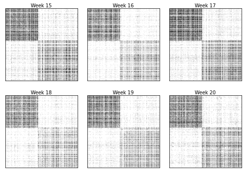
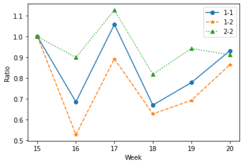
Figure 1: The left panel displays the adjacency matrices of 516 UK politicians over 6 weeks, where the structure with two communities is clear and stable. We then fit a multi-layer SBM model (Lei and Lin, 2022) and obtain the underlying network probability matrix $\bm{\widehat{P}}_{t}$ for each week. The right panel displays the ratios between each element of $\bm{\widehat{P}}_{t}$ over that of the first week. It is clear that $\bm{\widehat{P}}_{t}$ changes substantially from week to week.

In this paper, we consider dynamic networks with continuously changing connection probabilities, where the change points are defined as those when network structure changes substantially. In literature, only a few approaches (Cribben and Yu, 2017; Ozdemir et al., 2017; Cheung et al., 2020) are developed to detect such change points in dynamic networks, yet most are algorithm-based and lack theoretical justification. Specifically, Cheung et al. (2020) and Cribben and Yu (2017) need to estimate the community membership over a large number of sub-intervals, leading to heavy computational burden; and Ozdemir et al. (2017) requires several stringent and rather unrealistic constraints on the evolution of network subspace, which largely restricts its applicability.

We develop a change point detection method via subspace tracking, where each network layer is embedded in a low-dimensional subspace, and the network change points are detected by tracking the changes of the embedding subspace. Particularly, we introduce two novel detection statistics to jointly detect the subspace change points, one focusing on the bases of the subspaces and the other on their ranks. A refined detection algorithm is built upon these two detection statistics as well as some fine tuning to attain both theoretical guarantees and superior numerical performance in detecting the network subspace change points. To the best of our limited knowledge, the proposed method is the first network subspace change point detection method with theoretical guarantees. More convincingly, we also establish the impossibility region for detecting the network subspace change points for a minimax perspective, which essentially demonstrates that the proposed method is theoretically optimal up to a logarithm factor.

The rest of the paper is organized as follows. Section 2 presents the proposed method for detecting network subspace change points, and elucidates the detection algorithms. Section 3 establishes the asymptotic consistency of our proposed method and establishes the impossibility region for detecting the network subspace change points. Section 4 examines the numerical performance of the proposed method on both synthetic and real-world networks, and compares it against some existing competitors. A brief discussion is contained in Section 5, and the technical proofs are contained in the Appendix. The auxiliary lemmas can be found in the Supplementary Materials.

Notations.

For any positive integer $K$, denote $\{1,\ldots,K\}$ as $[K]$ for short. For any sequences $\{a_{n}\}_{n=1}^{\infty}$ and $\{b_{n}\}_{n=1}^{\infty}$, we write $a_{n}\prec b_{n}$ if $a_{n}=o(b_{n})$ and $a_{n}\preceq b_{n}$ if $a_{n}=O(b_{n})$. Further, if $a_{n}=O(b_{n})$ and $b_{n}=O(a_{n})$, we write $a_{n}\simeq b_{n}$. Denote by $e_{k}(K)$ the $k$-th standard orthonormal basis of $\mathbb{R}^{K}$, and $\bm{1}_{K}$ the $K$-dimensional vector of ones. For a square matrix $\bm{A}\in\mathbb{R}^{n\times n}$, its rank is denoted as $\text{rank}(\bm{A})$, its trace is denoted as $\text{tr}(\bm{A})$, and its eigenvalues can be sorted in a descending order $\lambda_{\max}\big{(}\bm{A}\big{)}=\lambda_{1}\big{(}\bm{A}\big{)}\geq\lambda_{2}\big{(}\bm{A}\big{)}\geq\cdots\geq\lambda_{n}\big{(}\bm{A}\big{)}=\lambda_{\min}\big{(}\bm{A}\big{)}$. Similarly, we also sort its singular value in a descending order $\sigma_{\max}\big{(}\bm{A}\big{)}=\sigma_{1}\big{(}\bm{A}\big{)}\geq\sigma_{2}\big{(}\bm{A}\big{)}\geq\cdots\geq\sigma_{n}\big{(}\bm{A}\big{)}=\sigma_{\min}\big{(}\bm{A}\big{)}$. Let $\bm{A}_{S,S^{\prime}}$ denote a submatrix of $\bm{A}$ with row indices in $S$ and column indices in $S^{\prime}$. For an orthonormal matrix $\bm{V}\in\mathbb{R}^{n\times m}$ with $n>m$, a basis of its orthogonal complement is denoted as $\bm{V}_{\perp}$.

2 Proposed method

For dynamic network $\{{\cal G}_{t}\}_{t=1}^{T}$, its symmetric adjacency matrix for each network layer is denoted as $\bm{A}_{t}\in\{0,1\}^{n\times n}$ with $\bm{P}_{t}=E(\bm{A}_{t})\in[0,1]^{n\times n}$. We consider a low-rank network embedding model (Arroyo et al., 2021),

$$\bm{P}_{t}=\rho_{n,T}\bm{V}_{t}\bm{M}_{t}\bm{V}_{t}^{\top},$$

where $\rho_{n,T}=\max_{t\in[T]}\|\bm{P}_{t}\|_{\max}$ controls the network sparsity that may vanish with $n$ and $T$, $\bm{M}_{t}\in\mathbb{R}^{R\times R}$ is a full-rank matrix, and $\bm{V}_{t}\in\mathbb{R}^{n\times R}$ is an orthonormal matrix. Apparently, $\bm{P}_{t}$ lies in the subspace spanned by the columns of $\bm{V}_{t}$, and it is identifiable up to an orthogonal transformation due to the full-rank $\bm{M}_{t}$.

Suppose there are a total of $K$ change points in $\{\bm{P}_{t}\}_{t=1}^{T}$, denoted as $\Gamma=\{\tau_{k}\}_{k=1}^{K}$ with $1=\tau_{0}<\tau_{1}<\cdots<\tau_{K}<\tau_{K+1}=T$, where

$${\bm{P}}_{t}=\rho_{n,T}\bm{V}^{(k)}\bm{M}_{t}(\bm{V}^{(k)})^{\top},$$ (1)

for any $t\in[\tau_{k-1},\tau_{k})$, and $\min_{k\in[K]}\|\bm{V}^{(k)}(\bm{V}^{(k)})^{\top}-\bm{V}^{(k+1)}(\bm{V}^{(k+1)})^{\top}\|_{F}>0$. It is important to remark that ${\bm{P}}_{t}$ may change continuously over time, whereas the latent subspace defined by $\bm{V}$ can only change at each $\tau_{k}$. A special case of (1) has been considered in Cheung et al. (2020), assuming $\bm{P}_{t}=\rho_{n,T}\bm{Z}^{(k)}\bm{B}_{t}(\bm{Z}^{(k)})^{\top}$ for any $t\in[\tau_{k-1},\tau_{k})$, where $\bm{Z}^{(k)}\in\{0,1\}^{n\times R}$ denotes the community membership. We term the change points defined in (1) as the network subspace change points, which are in sharp contrast to the network probability change points in literature (Wang et al., 2017; Bhattacharjee et al., 2020; Wang et al., 2021), which assumes that ${\bm{P}}_{t}$ can only change at each $\tau_{k}$ and otherwise remains constant within each $[\tau_{k-1},\tau_{k})$.

2.1 Two detection statistics

We first introduce two statistics to jointly detect the subspace change points of $\{\bm{P}_{t}\}_{t=1}^{T}$. The following auxiliary lemma is necessary.

Lemma 1.

Let $\bm{U}\in\mathbb{R}^{n\times R_{u}}$ and $\bm{V}\in\mathbb{R}^{n\times R_{v}}$ be two orthognormal matrices with $R_{u}+R_{v}\prec n$. It holds true for any $\bm{Q}\in\mathbb{R}^{R_{v}\times R_{v}}$ that

$$\|{\bm{U}}_{\perp}^{\top}\bm{V}\|_{2}^{2} \geq\big{(}R_{v}-R_{u}+\|\bm{U}\bm{U}^{\top}-\bm{V}\bm{V}^{\top}\|_{F}^{2}\big{)}/(2R_{v}),$$

$$\big{\|}{\bm{U}}_{\perp}^{\top}{\bm{V}}\bm{Q}\bm{V}^{\top}\big{\|}_{2} \geq\sigma_{\min}\big{(}\bm{Q}\big{)}\sqrt{\big{(}R_{v}-R_{u}+\|\bm{U}\bm{U}^{\top}-\bm{V}\bm{V}^{\top}\|_{2}^{2}\big{)}/(2R_{v})}.$$

Let $\Delta_{\min}=\min_{k\in[K+1]}(\tau_{k}-\tau_{k-1})$ denote the minimum distance between two adjacent change points. We examine the behavior of $\sum_{t=l-L+1}^{l}\bm{P}_{t}^{2}$ and $\sum_{t=l}^{l+L-1}\bm{P}_{t}^{2}$ with $L\leq\Delta_{\min}/3$, where summing up squared probability matrices has been proven to be effective in summarizing signals from multiple layers (Lei and Lin, 2022). Particularly, for any $\tau_{k-1}+2L\leq l<\tau_{k}+2L$, the first detection statistic measures the signal strength of projecting $\sum_{t=l-L+1}^{l}\bm{P}_{t}^{2}$ onto $\bm{V}_{\perp}^{(k)}$, defined as

$$\Pi_{proj}(l)=\Big{\|}(\bm{V}_{\perp}^{(k)})^{\top}\sum_{t=l-L+1}^{l}\bm{P}_{t}^{2}\Big{\|}_{2}.$$ (2)

It behaves differently before and after $\tau_{k}$, as long as $\text{rank}(\bm{V}^{(k+1)})\geq\text{rank}(\bm{V}^{(k)})$. Note that the scenario with $\text{rank}(\bm{V}^{(k+1)})<\text{rank}(\bm{V}^{(k)})$ also indicates a clear network subspace change point. Thus, with $R^{k}=\text{rank}(\bm{V}^{(k)})$, the second statistic is defined as

$$\Pi_{eig}(l)=\lambda_{R^{(k)}}\Big{(}\sum_{t=l}^{l+L-1}\bm{P}_{t}^{2}\Big{)}.$$ (3)

These two detection statistics can work jointly to detect the network subspace change points in $\{\bm{P}_{t}\}_{t=1}^{T}$. Specifically, when $\tau_{k-1}+2L\leq l<\tau_{k}$, we have $\sum_{t=l-L+1}^{l}\bm{P}_{t}^{2}=\sum_{t=l-L+1}^{l}\bm{V}^{(k)}\bm{M}_{t}^{2}(\bm{V}^{(k)})^{\top}$, which lies in the column space of $\bm{V}^{(k)}$ and thus is orthogonal to $\bm{V}^{(k)}_{\perp}$. Moreover, as $\bm{M}_{t}$ is full rank, we have

$$\lambda_{R^{(k)}}\Big{(}\sum_{t=l}^{l+L-1}\bm{P}_{t}^{2}\Big{)}\geq\lambda_{R^{(k)}}\Big{(}\sum_{t=l}^{\min\{l+L-1,\tau_{k}-1\}}\bm{M}_{t}^{2}\Big{)}>0,$$

It thus holds true that $\Pi_{proj}(l)=0$ and $\Pi_{eig}(l)>0$ when $\tau_{k-1}+2L\leq l<\tau_{k}$. When $\tau_{k}\leq l<\tau_{k}+2L$, it follows from Lemma 1 that

$$\Pi_{proj}(l) =\Big{\|}(\bm{V}_{\perp}^{(k)})^{\top}\sum_{t=l-L+1}^{l}\bm{P}_{t}^{2}\Big{\|}_{2}=\rho_{n,T}^{2}\Big{\|}(\bm{V}_{\perp}^{(k)})^{\top}\bm{V}^{(k+1)}\sum_{t=\max\{\tau_{k},l-L+1\}}^{l}\bm{M}_{t}^{2}(\bm{V}^{(k+1)})^{\top}\Big{\|}_{2}$$

$$\geq\rho_{n,T}^{2}\lambda_{\min}\Big{(}\sum_{t=\max\{\tau_{k},l-L+1\}}^{l}\bm{M}_{t}^{2}\Big{)}\sqrt{(R^{(k+1)}-R^{(k)}+\delta^{k+1})/(2R^{(k+1)})}.$$

It immediately implies that $\Pi_{proj}(l)>0$ as long as $R^{(k+1)}-R^{(k)}\geq 0$. On the other hand, if $R^{(k)}>R^{(k+1)}$, then

$$\Pi_{eig}(l)=\lambda_{R^{(k)}}\Big{(}\sum_{t=l}^{l+L-1}\bm{P}_{t}^{2}\Big{)}=\lambda_{R^{(k)}}\Big{(}\bm{V}^{(k+1)}\sum_{t=l}^{l+L-1}\bm{M}_{t}^{2}(\bm{V}^{(k+1)})^{\top}\Big{)}=0.$$

Therefore, a time point $l$ is a network subspace change point if $\Pi_{proj}(\cdot)$ rises from $0$ at $l$ or $\Pi_{eig}(\cdot)$ drops to $0$ at $l$.

We now illustrate the utility of the two statistics for jointly detecting the network subspace change points in a toy example with $n=100$, $T=400$, and $\Gamma=\{101,201,301\}$. We generate $\bm{V}^{(1)},\ldots,\bm{V}^{4}$ such that $\text{rank}(\bm{V}^{(1)})>\text{rank}(\bm{V}^{(2)})<\text{rank}(\bm{V}^{(3)})=\text{rank}(\bm{V}^{(4)})$, so that the subspace ranks decrease, increase or remain unchanged at the three change points, respectively. We simply set $L=20$ and calculate the two statistics over the time interval $[41,340]$. The values of both statistics are summarized in Figure 2. It is clear that $\Pi_{eig}(l)$ drops towards 0 at $l=101$, and $\Pi_{proj}(l)$ rises away from 0 after $l=201$ and $301$, respectively. Therefore all three change points can be perfectly identified by examining the behavior of $\Pi_{proj}(l)$ and $\Pi_{eig}(l)$.

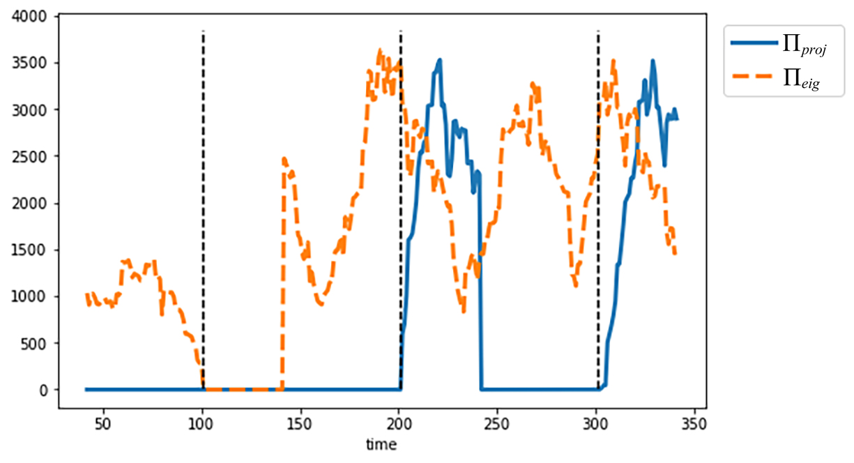
Figure 2: The curves of $\Pi_{proj}(l)$ and $\Pi_{eig}(l)$ for $l\in[41,340]$, and the dashed vertical lines mark the true change points at 101, 201, and 301.

2.2 Detection algorithm

The two proposed detection statistics in Section 2.1 lead to a simple recursive algorithm for detecting network subspace change points. Particularly, we first set $\widetilde{\tau}_{0}=1$. Given $\widetilde{\tau}_{k-1}$, for $l=\widetilde{\tau}_{k-1}+2L,\widetilde{\tau}_{k-1}+2L+1,\ldots$, we compute

$$\widehat{\Pi}_{proj}(l)=\Big{\|}(\widehat{\bm{V}}^{(k)}_{\perp})^{\top}\sum_{t=l-L+1}^{l}\big{(}\bm{A}_{t}^{2}-\bm{D}_{t}\big{)}\Big{\|}_{2}\ \ \mbox{and}\ \ \widehat{\Pi}_{eig}(l)=\lambda_{\text{rank}(\widehat{\bm{V}}^{(k)})}\bigg{(}\sum_{t=l}^{l+L-1}\bm{A}_{t}^{2}-\bm{D}_{t}\bigg{)}.$$ (4)

In both detection statistics, the unknown term $\bm{P}_{t}^{2}$ is replaced by its estimate $\bm{A}_{t}^{2}-\bm{D}_{t}$ with $\bm{D}_{t}=\text{diag}(\bm{A}_{t}\mathbf{1}_{n})$ (Lei and Lin, 2022), and $\widehat{\bm{V}}^{(k)}$ contains the leading eigenvectors of $\sum_{t=\widetilde{\tau}_{k-1}+L}^{\widetilde{\tau}_{k-1}+2L-1}(\bm{A}_{t}^{2}-\bm{D}_{t})$ with eigenvalues larger than a pre-specified thresholding value $b_{n,T}$. The first $l$ such that $\widehat{\Pi}_{proj}(l)>(1+\sqrt{2})b_{n,T}$ or $\widehat{\Pi}_{eig}(l)<b_{n,T}$ is set as the next estimated change point $\widetilde{\tau}_{k}$, and we repeat the above procedure for $l=\widetilde{\tau}_{k}+2L,\widetilde{\tau}_{k}+2L+1,\ldots$. The whole procedure continues until $l$ reaches $T-L$, and the resultant estimated change points are denoted as $\widetilde{\Gamma}=\{\widetilde{\tau}_{k}\}_{k=1}^{\widetilde{K}}$.

Note that these estimates rely heavily on the pre-specified threshold $b_{n,T}$, and thus an appropriate $b_{n,T}$ may yield sub-optimal detection of the network subspace change points in practice if the chosen $b_{n,T}$ is not suitable. We propose to further refine the detection algorithm, to be more robust against the choice of $b_{n,T}$. A universal eigenvalue threshold operator is defined as

$$\text{UEVT}\big{(}\bm{G},h\big{)}=\sum_{i:\lambda_{i}(\bm{G})>h}\lambda_{i}\big{(}\bm{G}\big{)}\bm{u}_{i}\bm{u}_{i}^{\top},$$

where $\bm{G}=\sum_{i=1}^{n}\lambda_{i}\big{(}\bm{G}\big{)}\bm{u}_{i}\bm{u}_{i}^{\top}$ denotes the standard eigen-decomposition of $\bm{G}$, and $h$ is a generic thresholding value. The UEVT operator constructs a low-rank approximation of $\bm{G}$ by excluding small eigenvalues and their associated eigenvectors. We consider a low-rank estimate for $\sum_{t=l-L+1}^{l}\bm{P}_{t}^{2}$,

$$\bm{\bar{P}}^{(l)}=\text{UEVT}\Big{(}\sum_{t=l-L+1}^{l}(\bm{A}_{t}^{2}-\bm{D}_{t}),b_{n,T}\Big{)},$$

whose rank is the cardinality of $\big{\{}i:\lambda_{i}\big{(}\sum_{t=l-L+1}^{l}(\bm{A}_{t}^{2}-\bm{D}_{t})\big{)}>b_{n,T}\big{\}}$. Then we introduce two additional statistics,

$$\widehat{\Pi}_{ref1}(l)=\text{tr}\big{(}\widehat{\bm{U}}_{\perp}^{(l-1)}(\widehat{\bm{U}}_{\perp}^{(l-1)})^{\top}\bar{\bm{P}}^{(l+L-1)}\big{)}\text{, and }\widehat{\Pi}_{ref2}(l)=\text{tr}\big{(}\widehat{\bm{U}}_{\perp}^{(l+L-1)}(\widehat{\bm{U}}_{\perp}^{(l+L-1)})^{\top}\bar{\bm{P}}^{(l-1)}\big{)},$$ (5)

where $\widehat{\bm{U}}^{(l-1)}$ and $\widehat{\bm{U}}^{(l+L-1)}$ contain the eigenvectors corresponding to the nonzero eigenvalues of $\text{UEVT}(\sum_{t=l-L}^{l-1}\bm{A}_{t}^{2}-\bm{D}_{t},b_{n,T})$ and $\text{UEVT}(\sum_{t=l}^{l+L-1}\bm{A}_{t}^{2}-\bm{D}_{t},b_{n,T})$, respectively.

For each $k\in[\widetilde{K}]$, we can refine the estimation of the change points by maximizing $\widehat{\Pi}_{ref1}(l)$ or $\widehat{\Pi}_{ref2}(l)$ based on the comparison of $\widehat{R}^{(k)}$ and $\widehat{R}^{(k+1)}$ in some range of $l$. Specifically, if $\widehat{R}^{(k)}<\widehat{R}^{(k+1)}$, it can be shown that the real change point $\tau_{k}^{*}$ is contained in $[\widetilde{\tau}_{k}-L+1,\widetilde{\tau}_{k}]$ with high probability. Then we denote the refined estimate as $\widehat{\tau}_{k}=\arg\max_{l\in[\widetilde{\tau}_{k}-L+1,\widetilde{\tau}_{k}]}\widehat{\Pi}_{ref1}(l)$. If $\widehat{R}^{(k)}>\widehat{R}^{(k+1)}$, it can be shown that $\tau_{k}^{*}$ is contained in $[\widetilde{\tau}_{k},\widetilde{\tau}_{k}+L-1]$ with high probability. Thus, we denote the refined estimate as $\widehat{\tau}_{k}=\arg\max_{l\in[\widetilde{\tau}_{k},\widetilde{\tau}_{k}+L-1]}\widehat{\Pi}_{ref2}(l)$. If $\widehat{R}^{(k)}=\widehat{R}^{(k+1)}$, we denote the first $l\in\{\widetilde{\tau}_{k}-1,\widetilde{\tau}_{k}-2,\cdots\}$ satisfying $\|(\widehat{\bm{V}}_{\perp}^{(k+1)})^{\top}\sum_{t=l}^{l+L-1}(\bm{A}_{t}^{2}-\bm{D}_{t})\|_{2}>(1+\sqrt{2})b_{n,T}$ as $\check{\tau}_{k}$. It can be shown that $\tau_{k}^{*}$ is contained in $[\check{\tau}_{k},\widetilde{\tau}_{k}]$ with high probability. Therefore, we set the refined estimate as $\widehat{\tau}_{k}=\arg\max_{l\in[\check{\tau}_{k},\widetilde{\tau}_{k}]}\widehat{\Pi}_{ref1}(l)$. The detailed detection algorithm is summarized in Algorithm 1.

Input: $b_{n,T}$ and $L$

1 Set $k=0$, $\widehat{\tau}_{k}=0$ and $l=2L+1$

2Set $\widehat{\bm{V}}_{\perp}^{(k+1)}$ as the eigenvectors of $\sum_{t=L+1}^{2L}(\bm{A}_{t}^{2}-\bm{D}_{t})$ with eigenvalues not larger than $b_{n,T}$

3while $l\leq T-L$  do

4       Calculate $\widehat{\Pi}_{proj}(l)$ and $\widehat{\Pi}_{eig}(l)$ by Eq.(4)

5      if $\widehat{\Pi}_{proj}(l)>(1+\sqrt{2})b_{n,T}$ or $\widehat{\Pi}_{eig}(l)<b_{n,T}$ then

6             Set $k=k+1$ and $\widetilde{\tau}_{k}=l$

7            Obtain $\widehat{\bm{V}}_{\perp}^{(k+1)}$ by selecting the eigenvectors of $\sum_{t=\widetilde{\tau}_{k}+L}^{\widetilde{\tau}_{k}+2L-1}(\bm{A}_{t}^{2}-\bm{D}_{t})$ with eigenvalues not larger than $b_{n,T}$

8            Set $l=\widetilde{\tau}_{k}+2L$

9      else

10            Set $l=l+1$

11      

12for $m=1,2,\cdots,\widehat{K}$ do

13       if $\text{rank}(\widehat{\bm{V}}^{m})<\text{rank}(\widehat{\bm{V}}^{m+1})$ then

14             Denote $\widehat{\tau}_{m}=\arg\max_{s\in[\widetilde{\tau}_{m}-L+1,\widetilde{\tau}_{m}]}\widehat{\Pi}_{ref1}(s)$, where $\widehat{\Pi}_{ref1}(s)$ is defined in Eq.(5)

15      if $\text{rank}(\widehat{\bm{V}}^{m})>\text{rank}(\widehat{\bm{V}}^{m+1})$ then

16             Denote $\widehat{\tau}_{m}=\arg\max_{s\in[\widetilde{\tau}_{m},\widetilde{\tau}_{m}+L-1]}\widehat{\Pi}_{ref2}(s)$, where $\widehat{\Pi}_{ref2}(s)$ is defined in Eq.(5)

17      if $\text{rank}(\widehat{\bm{V}}^{m})=\text{rank}(\widehat{\bm{V}}^{m+1})$ then

18             for $\check{\tau}_{m}=\widetilde{\tau}_{m}-1,\widetilde{\tau}_{m}-2,\cdots,\widehat{\tau}_{m-1}+1$ do

19                   if $\big{\|}(\widehat{\bm{V}}_{\perp}^{m+1})^{\top}\sum_{t=\check{\tau}_{m}}^{\check{\tau}_{m}+L-1}(\bm{A}_{t}^{2}-\bm{D}_{t})\big{\|}_{2}>(1+\sqrt{2})b_{n,T}$ then

20                        break

21                  

22            Denote $\widehat{\tau}_{m}=\arg\max_{s\in[\check{\tau}_{m},\widetilde{\tau}_{m}]}\widehat{\Pi}_{ref1}(s)$

23      

Output: $\widetilde{\Gamma}=\{\widetilde{\tau}_{1},\dots,\widetilde{\tau}_{\widetilde{K}}\}$ and $\widehat{\Gamma}=\{\widehat{\tau}_{1},\dots,\widehat{\tau}_{\widehat{K}}\}$ with $\widehat{K}=\widetilde{K}$

Algorithm 1 Subspace change point detection in dynamic networks

3 Theory

Let the true underlying probability matrices be $\{\bm{P}_{t}^{*}\}_{t=1}^{T}$, and the true change points be $\Gamma^{*}=\{\tau_{k}^{*}\}_{k=1}^{K^{*}}$ with $1=\tau_{0}^{*}<\tau_{1}^{*}<\cdots<\tau_{K^{*}}^{*}<\tau_{K^{*}+1}^{*}=T$. Then, for any $t\in[\tau_{k-1}^{*},\tau_{k}^{*})$, we have

$${\bm{P}}_{t}^{*}=\rho_{n,T}\bm{V}^{*(k)}\bm{M}_{t}^{*}(\bm{V}^{*(k)})^{\top}.$$

Denote the minimum distance $\Delta_{\min}^{*}=\min_{k\in[K^{*}+1]}(\tau_{k}^{*}-\tau_{k-1}^{*})$, and the minimum change magnitude $\delta_{\min}^{*}=\min_{k\in[K^{*}]}\delta^{*(k)}$ with $\delta^{*(k)}=\|\bm{V}^{*(k+1)}(\bm{V}^{*(k+1)})^{\top}-\bm{V}^{*(k)}(\bm{V}^{*(k)})^{\top}\|_{F}^{2}$. Note that $\delta_{\min}^{*}\leq 2\max_{k}R^{*(k)}\preceq 1$, where $R^{*(k)}=\text{rank}(\bm{V}^{*(k)})$. The following technical assumptions are made.

Assumption 1.

There exists a sequence $\alpha_{n}\preceq 1$ such that $\sigma_{\max}(\bm{M}_{t}^{*})\simeq\sigma_{\min}(\bm{M}_{t}^{*})\geq n\alpha_{n}$ for any $t\in[T]$.

Assumption 1 assures that $\bm{M}_{t}^{*}$ possesses balanced singular values, and its minimum singular value is asymptotically lowered bounded by $n\alpha_{n}$, where $\alpha_{n}$ may diminish to zero with $n$. This assumption is weaker than some commonly employed assumptions in network literature (Chen and Lei, 2018; Lei and Lin, 2022), which essentially implies Assumption 1 with $\alpha_{n}\simeq 1$.

Assumption 2.

(1) For dynamic networks with sparsity $\rho_{n,T}\succ 1/n$,

$$n\rho_{n,T}\alpha_{n}^{4}\Delta_{\min}^{*}\delta^{*}_{\min}\succ\big{(}\log(n+T)\big{)}^{2}.$$

(2) For dynamic networks with sparsity $\rho_{n,T}\preceq 1/n$,

$$n^{2}\rho_{n,T}^{2}\alpha_{n}^{4}\Delta_{\min}^{*}\delta^{*}_{\min}\succ\big{(}\log(n+T)\big{)}^{2}.$$

Assumption 2 specifies the required signal-to-noise ratio for the proposed method. Particularly, when the dynamic network is sparse with $\rho_{n,T}\simeq\log(n+T)/n$ and $\alpha_{n}\simeq 1$, Assumption 2 simplifies to $\Delta_{\min}^{*}\delta_{\min}^{*}\succ\log(n+T)$. Note that $\Delta_{\min}^{*}\delta_{\min}^{*}$ is a popular quantity to measure the difficulty of a change point detection problem (Yu, 2020). If we further require $\delta_{\min}^{*}\simeq 1$, then our proposed method only requires $\Delta_{\min}^{*}$ to be slightly larger than $\log(n+T)$, which is equivalent to the requirement in Wang et al. (2021) on network probability change point. When the dynamic network is extremely sparse with $\rho_{n,T}\simeq 1/n$ and $\alpha_{n}\simeq 1$, Assumption 2 simplifies to $\Delta_{\min}^{*}\delta_{\min}^{*}\succ\big{(}\log(n+T)\big{)}^{2}$, which is slightly stronger compared with the requirement when $\rho_{n,T}\simeq\log(n+T)/n$. In fact, our proposed method is still applicable even when $\rho_{n,T}\succ\log(n+T)/(n\sqrt{T})$, provided that $\alpha_{n}\simeq 1$, $\Delta_{\min}^{*}\simeq T$ and $\delta_{\min}^{*}\simeq 1$. This sparsity requirement matches up with some of the latest results in the literature of multi-layer stochastic block model (Lei et al., 2020; Lei and Lin, 2022).

Proposition 1.

Suppose Assumption 2 holds, then for any $l\in[T]\setminus[L]$ with $\Delta_{\min}^{*}\preceq L\leq\Delta_{\min}^{*}/3$, there exists positive constants $c_{1}$, $c_{2}$, and $c_{3}$ such that with probability at least $1-c_{1}(n+T)^{-2}$,it holds true that

$$\Big{\|}\sum_{t=l-L+1}^{l}\big{(}\bm{A}_{t}^{2}-\bm{D}_{t}-(\bm{P}_{t}^{*})^{2}\big{)}\Big{\|}_{2} \leq\frac{b_{n,T}}{\sqrt{\log(n+T)}},\text{ and }$$

$$\big{\|}\sum_{t=l-L+1}^{l}(\bm{P}_{t}^{*})^{2}-\bar{\bm{P}}^{(l)}\big{\|}_{F} \leq 4\max_{k\in[K^{*}+1]}\sqrt{R^{*(k)}}b_{n,T},$$

when $n+T$ is large enough, where $b_{n,T}=c_{2}\big{(}Ln\rho_{n,T}^{2}+L^{1/2}n\rho_{n,T}\sqrt{\max\{c_{3},n\rho_{n,T}\}}\big{)}\log(n+T)$.

Proposition 1 extends Theorem 3 and 5 in Lei and Lin (2022) to the context of dynamic networks with change points. It demonstrates that both $\sum_{t=l-L+1}^{l}(\bm{A}_{t}^{2}-\bm{D}_{t})$ and $\bar{\bm{P}}^{(l)}$ are good estimates of $\sum_{t=l-L+1}^{l}(\bm{P}_{t}^{*})^{2}$ under the spectral norm, whose estimation errors are controlled by the threshold $b_{n,T}$. These error bounds pave the theoretical foundation for quantifying the asymptotic behavior of the proposed methods.

Theorem 1.

Suppose Assumption 1 and all assumptions in Proposition 1 hold, and $n\succeq T$. Then it holds true that

$$\max_{k\in[K^{*}]}\frac{|\widehat{\tau}_{k}-{\tau}_{k}^{*}|}{\Delta_{\min}^{*}}\stackrel{{\scriptstyle p}}{{\rightarrow}}0.$$

Theorem 1 shows that the estimate $\widehat{\Gamma}$, with appropriate choices of $L$ and $b_{n,T}$, is a consistent estimate of $\Gamma^{*}$ in terms of both change point number and locations. Particularly, the larger $L$ is, the more network layers are integrated to calculate the detection statistics, yet it also increases bias in estimating $\widehat{\bm{V}}^{(k)}$, as the interval $[\widetilde{\tau}_{k}+L,\widetilde{\tau}_{k}+2L-1]$ may include networks from both sides of a change point $\tau_{k}^{*}$. Also, the value of $b_{n,T}$ depends on the network sparsity. When the networks are relatively dense with $n\rho_{n,T}\succ 1$, we shall set $b_{n,T}$ at the same magnitude of $L^{1/2}(n\rho_{n,T})^{3/2}\log(n+T)$; when the networks are extremely sparse with $n\rho_{n,T}\preceq 1$, $b_{n,T}$ shall be set at the same magnitude of $L^{1/2}n\rho_{n,T}\log(n+T)$.

Then, we establish an impossible regime in terms of $(\alpha_{n},\rho_{n,T},\Delta_{\min}^{*},\delta_{\min}^{*})$, where no change point detection algorithm is consistent in detecting $\{\tau_{k}^{*}\}_{k=1}^{K^{*}}$.

Theorem 2.

Let $\mathcal{Q}$ denote the class consisting of all multivariate Bernoulli distribution of $\{\bm{A}_{t}\}_{t=1}^{T}$. For any $Q\in\mathcal{Q}$, its corresponding probability matrices $\{\bm{P}_{t}^{(q)}\}_{t=1}^{T}$ must conform to Assumption 1, and the associated parameters satisfy $n\rho_{n,T}^{(q)}(\alpha_{n}^{(q)})^{4}\Delta_{\min}^{(q)}\delta_{\min}^{(q)}\simeq(\log(n+T))^{-1}$. Then there exists a sufficiently large $n_{0}$ and a positive constant $c_{4}$ such that for all $n\geq n_{0}$

$$\inf_{\check{\Gamma}}\sup_{Q\in\mathcal{Q}}\mathbb{E}_{Q}\Big{(}\frac{H\big{(}\check{\Gamma},\Gamma(Q)\big{)}}{\Delta_{\min}^{(q)}}\Big{)}\geq c_{4},$$

where $\check{\Gamma}$ can be any change point estimate, $\Gamma(Q)$ denotes the true network subspace change points under $Q\in\mathcal{Q}$, and $H(\cdot,\cdot)$ denotes the Hausdorff distance,

$$H\big{(}\check{\Gamma},\Gamma(Q)\big{)}=\max\Big{\{}\max_{\tau^{1}\in\Gamma(Q)}\min_{\tau^{2}\in\check{\Gamma}}|\tau^{1}-\tau^{2}|,\ \max_{\tau^{2}\in\check{\Gamma}}\min_{\tau^{1}\in\Gamma(Q)}|\tau^{1}-\tau^{2}|\Big{\}}.$$

Theorem 2 shows that, from a minimax perspective, there is no consistent change point detection algorithm if the parameters of the true underlying probability matrices $\{\bm{P}_{t}^{*}\}_{t=1}^{T}$ satisfy $n\rho_{n,T}\alpha_{n}^{4}\Delta_{\min}^{*}\delta_{\min}^{*}\preceq(\log(n+T))^{-1}$. It is interesting to remark that the proposed method is asymptotically consistent when $n\rho_{n,T}\succeq 1$ and $n\rho_{n,T}\alpha_{n}^{4}\Delta_{\min}^{*}\delta_{\min}^{*}\succ\big{(}\log(n+T)\big{)}^{2}$, which is optimal up to a logarithm factor in view of the impossible regime above.

Remark 1.

When $n\rho_{n,T}\prec 1$, Assumption 2 shall require an additional $(n\rho_{n,T})^{-1}$ term than the impossibility regime, which is possibly due to inherent challenge of estimating $\sum_{t=l-L+1}^{l}(\bm{P}_{t}^{*})^{2}$ and is a price to pay for not assuming the layer-wise positivity (Lei and Lin, 2022). If we further assume that all $\bm{P}_{t}^{*}$’s are non-negative definite, a slightly modified algorithm will exhibit consistency over the region complementary to the impossibility regime. Because we can replace the $\sum_{t=l-L+1}^{l}(\bm{P}_{t}^{*})^{2}$ with $\sum_{t=l-L+1}^{l}\bm{P}_{t}^{*}$ in (2) and (3), which can be accurately estimated using $\sum_{t=l-L+1}^{l}\bm{A}_{t}$ (Jing et al., 2021; Paul and Chen, 2020).

4 Numerical experiments

This section examines the numerical performance of the proposed method in various simulated examples and a real-life dynamic social media network dataset, and compare it against three existing methods, including a tensor subspace tracking approach (Ozdemir et al., 2017), a slightly modified spectral clustering method (Cribben and Yu, 2017) and a minimum description length based method (Cheung et al., 2020). For simplicity, we denote our proposed method as SCP, its refined version as rSCP, and the three competing methods as TST, SCM, and MDL, respectively. The tuning parameters of TST, SCM and MDL are set as in $\widehat{\tau}_{k}<\tau_{k}^{*}$, Cribben and Yu (2017) and Cheung et al. (2020), whereas the tuning parameters of SCP and rSCP are set following the theoretical results in Section 3. Particularly, we set $L=\lfloor T/20\rfloor$ and $b_{n,T}=\big{(}Ln\check{\rho}_{n,T}^{2}+L^{1/2}n\check{\rho}_{n,T}\sqrt{\max\{50,n\rho_{n,T}\}}\big{)}\log(n+T)/30$, where $\check{\rho}_{n,T}=\max\big{\{}\sum_{t=1}^{T}A_{ijt}/T,1\leq i<j\leq n\big{\}}$.

The numerical performance of each method is measured via its accuracy in estimating the number and locations of the true subspace change points. Specifically, for any change point set $\Gamma$ with cardinality $K$, its estimation accuracy is measured by $|K-K^{*}|$ and the Hausdorff distance.

4.1 Simulation

In all simulated examples, a total of $T$ networks are generated from the dynamic stochastic block model with three change points, denoted as $\Gamma^{*}=\{sT,1/2T,3/4T\}$, where $s\in[0,1/4]$ controls the minimum distance $\Delta_{\min}^{*}$, and $\Delta_{\min}^{*}$ will be larger when $s$ increases. For each sub-interval, we generate $\bm{P}_{t}^{*}=\rho_{n,T}\bm{Z}^{(k)}\bm{B}_{t}(\bm{Z}^{(k)})^{\top}$ for $k=1,\ldots,4$, where $\bm{Z}^{(k)}\in\{0,1\}^{n\times R^{k}}$ represents the cluster membership matrix, $\bm{B}_{t}\in[0,1]^{R^{k}\times R^{k}}$ represents the connectivity matrix, and $\rho_{n,T}$ controls the sparsity of the network. To construct $\bm{Z}^{(1)}$, we randomly assign the $n$ nodes into three clusters, where each cluster consists of $0.3n$, $0.3n$, and $0.4n$ nodes, respectively. Next, we randomly choose $q$ percent of the $n$ nodes and reassign them to a different cluster to create $\bm{Z}^{(2)}$. To construct $\bm{Z}^{(3)}$, we remove the smallest cluster from $\bm{Z}^{(2)}$ and reassign its nodes into the remaining two clusters. Finally, we set $\bm{Z}^{(4)}=\bm{Z}^{(2)}$. For any $t\in[T]\setminus[\tau_{2}^{*},\tau_{3}^{*})$, we randomly choose $\bm{B}_{t}$ in $\{\bm{B}^{1},\bm{B}^{2}\}$ with

$$\bm{B}^{1}=\bm{W}_{1}\text{diag}(1,0.5,0.5)\bm{W}_{1}^{T}\text{, and }\bm{B}^{2}=\bm{W}_{2}\text{diag}(1,0.5,-0.5)\bm{W}_{2}^{T},$$

where

$$\bm{W_{1}}=\left[\begin{array}[]{ccc}3/4&1/4&\sqrt{6}/4\\ 1/2&3/4&-\sqrt{6}/4\\ \sqrt{6}/4&-\sqrt{6}/4&-1/2\\ \end{array}\right]\text{, and }\bm{W_{2}}=\left[\begin{array}[]{ccc}1/2&1/2&-\sqrt{2}/2\\ 1/2&1/2&\sqrt{2}/2\\ \sqrt{2}/2&-\sqrt{2}/2&0\\ \end{array}\right].$$

For $t\in[\tau_{2}^{*},\tau_{3}^{*})$, we randomly choose $\bm{B}_{t}$ from $(\bm{B}^{1})_{[2],[2]}$ or $(\bm{B}^{2})_{[2],[2]}$, which are the $2\times 2$ upper left sub-matrices of $\bm{B}^{1}$ or $\bm{B}^{2}$. We consider three scenarios with various values of $\rho_{n,T}$, $q$ and $s$ to evaluate the performance of the proposed method in different aspects.

Scenario I: We fix $\rho_{n,T}=1$, $q=0.5$, but vary the minimum distance $s$ in $\{1/10,1/15,1/20\}$.

Scenario II: We fix $\rho_{n,T}=1$, $s=1/4$, but vary the minimum change magnitude $q$ in $\{0.3,0.2,0.1\}$.

Scenario III: We fix $q=0.5$, $s=1/4$, but vary network sparsity $\rho_{n,T}$ in $\{80/n,50/n,30/n\}$.

In each scenario, we present the averaged estimated change point numbers and the averaged Hausdorff distances obtained by different methods across 50 independent replications in Tables 1(b)-3(b). The symbol ‘/’ is used to signify that a method fails to produce any results within 24 hours.

Table 1: Averaged performance of different methods for estimating the number and locations of change points over 50 independent replications in Scenario I. The best performer is boldfaced.

(a) Number

	$s$	SCP	rSCP	SCM	TST	MDL
$n=100$ $T=200$	$1/10$	$\bm{0.00(0.00)}$	$\bm{0.00(0.00)}$	$6.48(0.48)$	$0.98(0.12)$	$0.80(0.12)$
	$1/15$	$\bm{0.00(0.00)}$	$\bm{0.00(0.00)}$	$8.78(0.56)$	$1.16(0.12)$	$0.52(0.08)$
	$1/20$	$\bm{0.00(0.00)}$	$\bm{0.00(0.00)}$	$9.58(0.59)$	$1.20(0.15)$	$0.84(0.10)$
$n=200$ $T=200$	$1/10$	$\bm{0.00(0.00)}$	$\bm{0.00(0.00)}$	$5.98(0.50)$	$0.98(0.10)$	$0.84(0.14)$
	$1/15$	$\bm{0.00(0.00)}$	$\bm{0.00(0.00)}$	$8.70(0.54)$	$0.96(0.07)$	$0.82(0.10)$
	$1/20$	$\bm{0.00(0.00)}$	$\bm{0.00(0.00)}$	$9.80(0.57)$	$0.92(0.07)$	$0.82(0.10)$
$n=400$ $T=300$	$1/10$	$\bm{0.00(0.00)}$	$\bm{0.00(0.00)}$	/	$0.92(0.08)$	/
	$1/15$	$\bm{0.00(0.00)}$	$\bm{0.00(0.00)}$	/	$0.84(0.05)$	/
	$1/20$	$\bm{0.00(0.00)}$	$\bm{0.00(0.00)}$	/	$0.88(0.07)$	/

(b) Location

	$s$	SCP	rSCP	SCM	TST	MDL
$n=100$ $T=200$	$1/10$	$2.56(0.08)$	$\bm{0.10(0.04)}$	$27.32(0.89)$	$28.36(1.73)$	$15.82(1.62)$
	$1/15$	$7.00(0.00)$	$\bm{0.38(0.14)}$	$28.94(1.00)$	$29.12(1.68)$	$15.08(1.55)$
	$1/20$	$10.00(0.00)$	$\bm{2.88(0.09)}$	$31.00(1.01)$	$29.54(1.70)$	$15.36(1.44)$
$n=200$ $T=200$	$1/10$	$1.74(0.06)$	$\bm{0.04(0.03)}$	$27.80(0.97)$	$32.52(1.66)$	$21.82(1.94)$
	$1/15$	$7.00(0.00)$	$\bm{0.08(0.04)}$	$30.60(0.93)$	$32.40(1.74)$	$22.82(1.69)$
	$1/20$	$10.00(0.00)$	$\bm{2.02(0.02)}$	$31.70(0.98)$	$34.00(1.62)$	$21.40(2.32)$
$n=400$ $T=300$	$1/10$	$1.28(0.06)$	$\bm{0.00(0.00)}$	/	$54.44(3.02)$	/
	$1/15$	$10.00(0.00)$	$\bm{0.10(0.04)}$	/	$55.88(2.82)$	/
	$1/20$	$15.00(0.00)$	$\bm{2.00(0.00)}$	/	$52.78(3.28)$	/

Table 2: Averaged performance of different methods for estimating the number and locations of change points over 50 independent replications in Scenario II. The best performer is boldfaced.

(a) Number

	$q$	SCP	rSCP	SCM	TST	MDL
$n=100$ $T=50$	$0.3$	$\bm{0.00(0.00)}$	$\bm{0.00(0.00)}$	$2.48(0.11)$	$0.42(0.07)$	$0.72(0.09)$
	$0.2$	$\bm{0.00(0.00)}$	$\bm{0.00(0.00)}$	$2.50(0.09)$	$0.46(0.07)$	$0.82(0.09)$
	$0.1$	$\bm{0.02(0.02)}$	$\bm{0.02(0.02)}$	$2.78(0.07)$	$0.48(0.07)$	$0.88(0.11)$
$n=200$ $T=100$	$0.3$	$\bm{0.00(0.00)}$	$\bm{0.00(0.00)}$	$1.46(0.13)$	$0.86(0.05)$	$0.72(0.08)$
	$0.2$	$\bm{0.00(0.00)}$	$\bm{0.00(0.00)}$	$1.40(0.14)$	$0.64(0.07)$	$0.82(0.13)$
	$0.1$	$\bm{0.00(0.00)}$	$\bm{0.00(0.00)}$	$1.92(0.14)$	$0.84(0.05)$	$0.52(0.09)$
$n=100$ $T=500$	$0.3$	$\bm{0.00(0.00)}$	$\bm{0.00(0.00)}$	/	$1.24(0.15)$	/
	$0.2$	$\bm{0.00(0.00)}$	$\bm{0.00(0.00)}$	/	$1.26(0.17)$	/
	$0.1$	$\bm{0.00(0.00)}$	$\bm{0.00(0.00)}$	/	$1.26(0.14)$	/

(b) Location

	$q$	SCP	rSCP	SCM	TST	MDL
$n=100$ $T=50$	$0.3$	$0.94(0.04)$	$\bm{0.16(0.05)}$	$20.44(0.88)$	$9.48(0.10)$	$7.90(0.48)$
	$0.2$	$1.04(0.04)$	$\bm{0.04(0.03)}$	$19.94(0.89)$	$9.54(0.07)$	$7.86(0.53)$
	$0.1$	$1.64(0.25)$	$\bm{0.46(0.32)}$	$22.88(0.65)$	$9.52(0.07)$	$8.00(0.53)$
$n=200$ $T=100$	$0.3$	$1.06(0.03)$	$\bm{0.02(0.02)}$	$25.30(1.36)$	$14.52(0.54)$	$13.86(1.04)$
	$0.2$	$1.18(0.05)$	$\bm{0.00(0.00)}$	$28.54(1.64)$	$13.62(0.57)$	$13.12(0.95)$
	$0.1$	$1.76(0.06)$	$\bm{0.00(0.00)}$	$32.82(1.90)$	$14.30(0.58)$	$11.50(0.89)$
$n=100$ $T=500$	$0.3$	$6.34(0.13)$	$\bm{0.02(0.02)}$	/	$58.78(6.30)$	/
	$0.2$	$7.14(0.16)$	$\bm{0.02(0.02)}$	/	$55.86(6.14)$	/
	$0.1$	$9.02(0.18)$	$\bm{0.00(0.00)}$	/	$54.76(5.92)$	/

Table 3: Averaged performance of different methods for estimating the number and locations of change points over 50 independent replications in Scenario III. The best performer is boldfaced.

(a) Number

	$\rho_{n,T}$	SCP	rSCP	SCM	TST	MDL
$n=100$ $T=150$	$80/n$	$\bm{0.00(0.00)}$	$\bm{0.00(0.00)}$	$2.28(0.26)$	$1.08(0.13)$	$1.36(0.17)$
	$50/n$	$\bm{0.00(0.00)}$	$\bm{0.00(0.00)}$	$2.24(0.32)$	$2.40(0.17)$	$1.06(0.15)$
	$30/n$	$\bm{0.02(0.02)}$	$\bm{0.02(0.02)}$	$2.20(0.30)$	$4.24(0.15)$	$1.28(0.14)$
$n=100$ $T=300$	$80/n$	$\bm{0.00(0.00)}$	$\bm{0.00(0.00)}$	$3.96(0.41)$	$2.10(0.20)$	$1.30(0.20)$
	$50/n$	$\bm{0.00(0.00)}$	$\bm{0.00(0.00)}$	$4.18(0.42)$	$3.50(0.25)$	$2.14(0.25)$
	$30/n$	$\bm{0.00(0.00)}$	$\bm{0.00(0.00)}$	$3.82(0.42)$	$4.48(0.33)$	$2.94(0.31)$
$n=400$ $T=400$	$80/n$	$\bm{0.00(0.00)}$	$\bm{0.00(0.00)}$	/	$1.54(0.18)$	/
	$50/n$	$\bm{0.00(0.00)}$	$\bm{0.00(0.00)}$	/	$2.84(0.27)$	/
	$30/n$	$\bm{0.00(0.00)}$	$\bm{0.00(0.00)}$	/	$9.20(0.46)$	/

(b) Location

	$\rho_{n,T}$	SCP	rSCP	SCM	TST	MDL
$n=100$ $T=150$	$80/n$	$2.36(0.07)$	$\bm{0.16(0.06)}$	$27.40(1.69)$	$24.20(1.32)$	$15.88(1.20)$
	$50/n$	$3.42(0.09)$	$\bm{0.40(0.09)}$	$30.04(1.33)$	$21.48(1.06)$	$14.68(1.29)$
	$30/n$	$5.54(0.41)$	$\bm{1.02(0.18)}$	$29.90(1.83)$	$23.66(0.82)$	$15.20(1.14)$
$n=100$ $T=300$	$80/n$	$4.08(0.07)$	$\bm{0.18(0.05)}$	$46.32(2.50)$	$27.50(1.69)$	$18.64(1.68)$
	$50/n$	$5.30(0.11)$	$\bm{0.26(0.07)}$	$45.08(2.33)$	$32.22(1.98)$	$25.86(2.10)$
	$30/n$	$7.40(0.14)$	$\bm{0.84(0.16)}$	$51.08(2.30)$	$36.58(2.22)$	$29.34(2.54)$
$n=400$ $T=400$	$80/n$	$6.42(0.14)$	$\bm{0.30(0.07)}$	/	$24.78(2.22)$	/
	$50/n$	$9.26(0.15)$	$\bm{0.20(0.06)}$	/	$35.16(2.71)$	/
	$30/n$	$15.02(0.24)$	$\bm{0.48(0.09)}$	/	$83.76(0.76)$	/

It is evident from Table 1(b)-3(b) that SCP and rSCP perform significantly better than the other three methods in terms of both change point number and location recovery. More importantly, our refined estimate consistently outperforms the original one across all scenarios, exhibiting a significant improvement ranging from $72\%$ to $100\%$ in terms of location estimation errors. When $n$ and $T$ are held constant, we observe that the performance of SCP deteriorates as $s$, $q$, or $\rho_{n,T}$ decreases. This degradation can be attributed primarily to the increased difficulty of the problem. Compared to SCP, rSCP demonstrates greater resilience to variations in these three parameters in most scenarios, validating the robustness of our refined procedure. In Table 1(b), we observe that rSCP clearly benefits from the increasing of node number $n$. In Table 2(b) and 3(b), especially when $q$ or $\rho_{n,T}$ is extremely small, rSCP can locate the change point more accurately under larger $T$. This demonstrates the importance of effectively integrating the information across network layers and boosting the signal, which is largely overlooked by the other three comparison methods. Generally speaking, MDL performs slightly better than SCM and TST. However, its computational complexity is exceedingly high, resulting in computation times that are hundreds of times longer than our methods.

4.2 UK politician social network

We now apply the proposed rSCP method to detect change points in the dynamic social networks of UK politicians (Weaver et al., 2018). It collects Twitter interactions among 648 UK politicians, including both Members of Parliament and British Members of the European Parliament, during December 12, 2014 to August 8, 2016. Each layer of network records whether the politicians interact with each other within a one-week interval, leading to a dynamic network with 85 layers. Among the politicians, 516 of them were from the Conservative or Labour parties, who had connected with others at least once within the whole 85 weeks.

Our method detects six change points, summarized in Figure LABEL:fig:change_point. The second, third, fourth and sixth detected change points well align with the major political events: the 2015 General Election, the 2015 Labour Leadership Voting, and the announcement and conclusion of the 2016 European Union membership referendum (EU referendum).

It is also interesting to remark that the politicians do not interact much on Twitter before the first change point, and the rank of the estimated network subspace is just one. Soon after, as it is approaching the 2015 General Election day, the politicians leading left or right had started to interact within their communities. The rank of the estimated network subspace increases to two, and the estimated two communities agree with the political affiliations of politicians: $90\%$ of the members in the first community belong to the Conservative party, and the second community consists of Labour party members only. It is evident that the social separation between the Conservative and Labour party had become clearer after the first change point.

The fifth change point marks the time that the 2016 European Union membership referendum had become a dominant topic among UK politicians. Before the fifth change point, the estimated two communities primarily reflects the conflicts between the two parties. More specifically, approximately $85\%$ of the members in the first community are affiliated with the Conservative party, while the second community consists of the Labour Party members only. Notice that only seven Labour Party members voted ‘Leave’ in the EU referendum, and six of them are assigned to the first community, as the Conservative Party remains neutral during the EU referendum. As the referendum drawing became close, the three estimated communities are no longer associated with party affiliations, but significantly influenced by the politician’s stance on the referendum. Within the first community, labeled as ‘Leave’, $93.2\%$ of the politicians voted ‘Leave’ and $5.1\%$ voted ’Remain’. Within the second community, labeled as ‘Remain’, $9.2\%$ politicians voted ‘Leave’ and $87.7\%$ voted ‘Remain’. The third community, labeled as ‘Wavering’, interacts much more frequently with the other two communities rather than within itself.

As an interesting by-product, we observe that politicians within the ‘Leave’ community exhibit more intense interactions among themselves compared with the other two communities. We calculate the average internal density (Cong and Lee, 2022; Yang and Leskovec, 2012) for each community,

$$Acc_{k}=\sum_{\bm{c}_{i}=\bm{c}_{j}=k}\sum_{t=\widehat{\tau}_{5}}^{\widehat{\tau}_{6}-1}\frac{A_{t(i,j)}}{N_{k}(\widehat{\tau}_{6}-\widehat{\tau}_{5})},$$

where $k\in[3]$, $\bm{c}\in[3]^{512}$ represents the cluster membership and $N_{k}$ denotes the total number of the $k$-th community. The average internal density of the ‘Leave’ community is 0.6, which is notably higher than that of the other two communities, $0.27$ for ‘Remain’ and $0.16$ for ‘Wavering’. Moreover, we also calculate Cohen’s $\kappa$ index for each pair of the nodes under different snapshots, which is widely used to measure the similarity of node pairs (Hoffman et al., 2015, 2018). The indices are displayed in Figure 4, revealing that politicians within the ‘Leave’ community share more similar behaviors compared to the other two communities. Members of the ‘Leave’ community display higher levels of engagement in providing reciprocal support on social media, which offers some interesting insights into their success in the referendum.

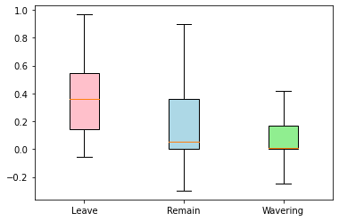
Figure 4: Boxplots of the Cohen’s $\kappa$ indices between node pairs within each community.

5 Conclusion

This article proposes a novel change point detection model for dynamic heterogeneous networks, which focuses on the alternation of the latent subspace but permits a continuous shift of the probability matrix. A sliding window algorithm with a refined procedure has been proposed to tackle this problem, where we define several novel statistics to quantify the subspace change. The effectiveness of our method is supported by various numerical experiments and asymptotic consistency in terms of change point detection. Particularly, the theoretical result can be established under nearly all parameters scaling for which this task is feasible. We believe this new change point detection model has broad application potential and can be extended to many more scenarios. One possible extension is to consider the node degree heterogeneity, which can continuously evolve over time.

Appendix A: Technical proofs

Proof of Lemma 1. Note that

$$\|\bm{UU}^{\top}-\bm{VV}^{\top}\|_{F}^{2} =\operatorname{tr}(\bm{UU}^{\top}+\bm{VV}^{\top}-\bm{UU}^{\top}\bm{VV}^{\top}-\bm{VV}^{\top}\bm{UU^{\top}})$$

$$=R_{u}+R_{v}-2\operatorname{tr}(\bm{V}^{\top}\bm{UU}^{\top}\bm{V}).$$ (6)

Then we have

$$\|\bm{U}_{\perp}^{\top}\bm{V}\|_{F}^{2}=\operatorname{tr}(\bm{V}^{\top}\bm{U}_{\perp}\bm{U}_{\perp}^{\top}\bm{V}) =\operatorname{tr}(\bm{V}^{\top}\bm{V})-\operatorname{tr}(\bm{V}^{\top}\bm{UU}^{\top}\bm{V})$$

$$=R_{v}-\big{(}R_{u}+R_{v}-\|\bm{UU}^{\top}-\bm{VV}^{\top}\|_{F}^{2}\big{)}/2$$

$$=\big{(}R_{v}-R_{u}+\|\bm{UU}^{\top}-\bm{VV}^{\top}\|_{F}^{2}\big{)}/2,$$

which directly leads to

$$\|\bm{U}_{\perp}^{\top}\bm{V}\|_{2}^{2}\geq\|\bm{U}_{\perp}^{\top}\bm{V}\|_{F}^{2}/R_{v}=\big{(}R_{v}-R_{u}+\|\bm{UU}^{\top}-\bm{VV}^{\top}\|_{F}^{2}\big{)}/(2R_{v}),$$

where the first inequality follows from the assumption that $R_{v}\prec n-R_{u}$.

We then turn to bound $\|\bm{U_{\perp}}^{\top}\bm{VQV}^{\top}\|_{2}$. First, we have

$$\|\bm{U_{\perp}}^{\top}\bm{VQV}^{\top}\|_{F}^{2} =\operatorname{tr}(\bm{U}_{\perp}^{\top}\bm{VQ}^{2}\bm{V}^{\top}\bm{U}_{\perp})=\operatorname{tr}\big{(}\bm{O}\text{diag}\big{(}\lambda_{1}\bm{(Q^{2})},\cdots,\lambda_{R_{v}}(\bm{Q^{2}})\big{)}\bm{O}^{\top}\bm{V}^{\top}\bm{U}_{\perp}\bm{U}_{\perp}^{\top}\bm{V}\big{)}$$

$$=\operatorname{tr}\big{(}\text{diag}\big{(}\lambda_{1}\bm{(Q^{2})},\cdots,\lambda_{R_{v}}(\bm{Q^{2}})\big{)}\bm{O}^{\top}\bm{V}^{\top}\bm{U}_{\perp}\bm{U}_{\perp}^{\top}\bm{VO}\big{)}$$

$$\geq\lambda_{\min}(\bm{Q}^{2})\operatorname{tr}\big{(}\bm{O}^{\top}\bm{V}^{\top}\bm{U}_{\perp}\bm{U}_{\perp}^{\top}\bm{VO}\big{)}=\lambda_{\min}(\bm{Q}^{2})\|\bm{U}_{\perp}^{\top}\bm{V}\|_{F}^{2},$$ (7)

where $\bm{O}\text{diag}\big{(}\lambda_{1}\bm{(Q^{2})},\cdots,\lambda_{R_{v}}(\bm{Q^{2}})\big{)}\bm{O}^{\top}$ is the eigen-decomposition of $\bm{Q}^{2}$. It then follows that

$$\big{\|}{\bm{U}}_{\perp}^{\top}{\bm{V}}\bm{Q}\bm{V}^{\top}\big{\|}_{2}\geq R_{v}^{-1/2}\big{\|}{\bm{U}}_{\perp}^{\top}{\bm{V}}\bm{Q}\bm{V}^{\top}\big{\|}_{F}\geq\sigma_{\min}\big{(}\bm{Q}\big{)}\sqrt{\big{(}R_{v}-R_{u}+\|\bm{U}\bm{U}^{\top}-\bm{V}\bm{V}^{\top}\|_{F}^{2}\big{)}/(2R_{v})}.$$

This completes the proof of Lemma 1. $\blacksquare$

Proof of Proposition 1. First, it follows from the triangle inequality that

$$\ \Big{\|}\sum_{t=l-L+1}^{l}\big{(}\bm{A}_{t}^{2}-\bm{D}_{t}-(\bm{P}_{t}^{*})^{2}\big{)}\Big{\|}_{2}$$

$$= \Big{\|}\sum_{t=l-L+1}^{l}\big{(}(\bm{A}_{t}-\bm{P}_{t}^{*})^{2}+\bm{A}_{t}\bm{P}_{t}^{*}+\bm{P}_{t}^{*}\bm{A}_{t}-2(\bm{P}_{t}^{*})^{2}-\bm{D}_{t}\big{)}\Big{\|}_{2}$$

$$\leq \ 2\Big{\|}\sum_{t=l-L+1}^{l}(\bm{A}_{t}-\bm{P}_{t}^{*})\bm{P}_{t}^{*}\Big{\|}_{2}+\Big{\|}\sum_{t=l-L+1}^{l}\text{diag}\big{(}(\bm{A}_{t}-\bm{P}_{t}^{*})^{2}\big{)}-\bm{D}_{t}\Big{\|}_{2}$$

$$\hskip 110.00017pt+\Big{\|}\sum_{t=l-L+1}^{l}(\bm{A}_{t}-\bm{P}_{t}^{*})^{2}-\text{diag}\big{(}(\bm{A}_{t}-\bm{P}_{t})^{2}\big{)}\Big{\|}_{2}.$$ (8)

Since $\alpha_{n}\preceq 1$, $\delta_{\min}^{*}\preceq 1$ and $\Delta_{\min}^{*}\preceq L$, it then follows from Assumption 2 that $n\rho_{n,T}\sqrt{L}\succeq n\rho_{n,T}\alpha_{n}^{2}\sqrt{\Delta_{\min}^{*}}\delta_{\min}^{*}\succ\log(n+T)$, when $\rho_{n,T}\preceq 1/n$. When $n\rho_{n,T}\succ 1$, we also have $n\rho_{n,T}\sqrt{L}\succ\max\{\sqrt{\Delta_{\min}^{*}},\big{(}\log(n+T)\big{)}^{2}/\sqrt{\Delta_{\min}^{*}}\}\succeq\log(n+T)$. Then, with probability at least $1-c_{1}(n+T)^{-2}$, it holds true that

$$\Big{\|}\sum_{t=l-L+1}^{l}(\bm{A}_{t}-\bm{P}_{t}^{*})\bm{P}_{t}^{*}\Big{\|}_{2} \leq\frac{c_{2}}{4}(n\rho_{n,T})^{3/2}\sqrt{L\log(n+T)},$$

$$\Big{\|}\sum_{t=l-L+1}^{l}\text{diag}\big{(}(\bm{A}_{t}-\bm{P}_{t})^{2}\big{)}-\bm{D}_{t}\Big{\|}_{2} \leq c_{2}Ln\rho_{n,T}^{2},\ \mbox{and}$$

$$\Big{\|}\sum_{t=l-L+1}^{l}(\bm{A}_{t}-\bm{P}_{t})^{2}-\text{diag}\big{(}(\bm{A}_{t}-\bm{P}_{t})^{2}\big{)}\Big{\|}_{2} \leq\frac{c_{2}}{4}n\rho_{n,T}(\sqrt{n\rho_{n,T}}+c_{3})\sqrt{L\log(n+T)},$$

where the first two inequalities directly follow from Appendix C of Lei and Lin (2022), and the last inequality follows from (A.13)-(A.15) in Appendix B of Lei and Lin (2022) with slight modification. The first desired inequality in Proposition 1 then follows immediately.

Next, we turn to derive the second inequality on $\big{\|}\sum_{t=l-L+1}^{l}(\bm{P}_{t}^{*})^{2}-\bar{\bm{P}}^{(l)}\big{\|}_{F}$, which can be upper bounded by $\sqrt{\text{rank}\big{(}\sum_{t=l-L+1}^{l}(\bm{P}_{t}^{*})^{2}\big{)}+\text{rank}\big{(}\bar{\bm{P}}^{(l)}\big{)}}\big{\|}\sum_{t=l-L+1}^{l}(\bm{P}_{t}^{*})^{2}-\bar{\bm{P}}^{(l)}\big{\|}_{2}$. Since $L<\Delta_{\min}^{*}$, there exists at most one change point in $[l-L+1,l]$ resulting in $\text{rank}\big{(}\sum_{t=l-L+1}^{l}(\bm{P}_{t}^{*})^{2}\big{)}\leq 2\max_{k\in[K^{*}+1]}R^{*(k)}$. Following from Weyl’s inequality, with probability at least $1-c_{1}(n+T)^{-2}$, it holds true that

$$\lambda_{2\max_{k\in[K^{*}+1]}R^{*(k)}+1}\Big{(}\sum_{t=l-L+1}^{l}\big{(}\bm{A}_{t}^{2}-\bm{D}_{t}\big{)}\Big{)}$$

$$\leq\ \lambda_{2\max_{k\in[K^{*}+1]}R^{*(k)}+1}\Big{(}\sum_{t=l-L+1}^{l}(\bm{P}_{t}^{*})^{2}\Big{)}+\Big{\|}\sum_{t=l-L+1}^{l}\big{(}\bm{A}_{t}^{2}-\bm{D}_{t}-(\bm{P}_{t}^{*})^{2}\big{)}\Big{\|}_{2}<b_{n,T},$$

which further implies that the rank of $\bar{\bm{P}}^{(l)}$ is at most $2\max_{k\in[K^{*}+1]}R^{*(k)}$. Then, we have

$$\Big{\|}\sum_{t=l-L+1}^{l}(\bm{P}_{t}^{*})^{2}-\bar{\bm{P}}^{(l)}\Big{\|}_{F}\leq 2\max_{k\in[K^{*}+1]}\sqrt{R^{*(k)}}\Big{\|}\sum_{t=l-L+1}^{l}(\bm{P}_{t}^{*})^{2}-\bar{\bm{P}}^{(l)}\Big{\|}_{2}$$

$$\leq\ 2\max_{k\in[K^{*}+1]}\sqrt{R^{*(k)}}\bigg{(}\Big{\|}\sum_{t=l-L+1}^{l}\big{(}\bm{A}_{t}^{2}-\bm{D}_{t}\big{)}-\bar{\bm{P}}^{(l)}\Big{\|}_{2}+\Big{\|}\sum_{t=l-L}^{l}\big{(}\bm{A}_{t}^{2}-\bm{D}_{t}-(\bm{P}_{t}^{*})^{2}\big{)}\Big{\|}_{2}\bigg{)}$$

$$\leq\ 4\max_{k\in[K^{*}+1]}\sqrt{R^{*(k)}}b_{n,T}.$$

This completes the proof of Proposition 1. $\blacksquare$

Proof of Theorem 1. For $L\leq l\leq T-L+1$, we consider the event

$$\mathcal{B}_{l}=\bigg{\{}\Big{\|}\sum_{t=l-L+1}^{l}\big{(}\bm{A}_{t}^{2}-\bm{D}_{t}-(\bm{P}_{t}^{*})^{2}\big{)} \Big{\|}_{2}\leq b_{n,T}/\sqrt{\log(n+T)},$$

$$\text{and }\Big{\|}\sum_{t=l-L+1}^{l}(\bm{P}_{t}^{*})^{2}-\bar{\bm{P}}^{(l)}\Big{\|}_{F}\leq 4\max_{k\in[K^{*}+1]}\sqrt{R^{*(k)}}b_{n,T}\bigg{\}}.$$

By Proposition 1, we have $\mathbb{P}\big{(}\mathcal{B}_{l}\big{)}\geq 1-c_{1}(n+T)^{-2}$ for each $l$. Define the event $\mathcal{B}$ to be the intersection of $\{\mathcal{B}_{l}\}_{l=L}^{T-L+1}$, and then

$$\mathbb{P}\big{(}\mathcal{B}\big{)}=1-\mathbb{P}\big{(}\mathcal{B}^{c}\big{)}=\mathbb{P}\big{(}\cup_{l\in[L,T-L+1]}\mathcal{B}_{l}^{c}\big{)}\geq 1-\sum_{l\in[L,T-L+1]}\mathbb{P}\big{(}\mathcal{B}_{l}^{c}\big{)}\geq 1-c_{1}(n+T)^{-1}.$$

We then proceed to prove Theorem 1 conditional on the event $\mathcal{B}$.

For any $k\in[K^{*}]$, we first consider the scenario with $R^{*(k)}<R^{*(k+1)}$. Under event $\mathcal{B}$, Lemma 2 implies that $\widetilde{\tau}_{k}\geq\tau_{k}^{*}$ and $|\widetilde{\tau}_{k}-\tau_{k}^{*}|\prec L$. As a consequence, if $\widehat{\tau}_{k}\geq\tau_{k}^{*}$, we immediately have $\widehat{\tau}_{k}-\tau_{k}^{*}\leq\widetilde{\tau}_{k}-\tau_{k}^{*}\prec L$. If $\widehat{\tau}_{k}<\tau_{k}^{*}$, for any $l\in[\widetilde{\tau}_{k}-L+1,\tau_{k}^{*}]$, it can be shown conditional on $\mathcal{B}$ that

$$\lambda_{R^{*(k)}}\bigg{(}\sum_{t=l-L}^{l-1}\bm{A}_{t}^{2}-\bm{D}_{t}\bigg{)} \geq\lambda_{R^{*(k)}}\bigg{(}\sum_{t=l-L}^{l-1}(\bm{P}_{t}^{*})^{2}\bigg{)}-\bigg{\|}\sum_{t=l-L}^{l-1}\big{(}\bm{A}_{t}^{2}-\bm{D}_{t}-(\bm{P}_{t}^{*})^{2}\big{)}\bigg{\|}_{2}$$

$$\geq Ln^{2}\alpha_{n}^{2}\rho_{n,T}^{2}-b_{n,T}/\sqrt{\log(n+T)},$$

where the second inequality follows from Assumption 1 and Proposition 1. Further,

$$\frac{b_{n,T}}{Ln^{2}\alpha_{n}^{2}\rho_{n,T}^{2}} =\frac{c_{2}\left(Ln\rho_{n,T}^{2}+\sqrt{L}n\rho_{n,T}\max\left\{\sqrt{n\rho_{n,T}},c_{3}\right\}\right)\log(n+T)}{Ln^{2}\alpha_{n}^{2}\rho_{n,T}^{2}}$$

$$\preceq\frac{\sqrt{L}n\rho_{n,T}\log(n+T)}{Ln^{2}\alpha_{n}^{2}\rho_{n,T}^{2}}+\frac{\sqrt{L}n^{3/2}\rho_{n,T}^{3/2}\log(n+T)}{Ln^{2}\alpha_{n}^{2}\rho_{n,T}^{2}}$$

$$\preceq\frac{\log(n+T)}{\sqrt{\Delta_{\min}^{*}}n\rho_{n,T}\alpha_{n}^{2}}+\frac{\log(n+T)}{\sqrt{\Delta_{\min}^{*}n\rho_{n,T}}\alpha_{n}^{2}}\prec 1,$$ (9)

where the first inequality follows from $Ln\rho_{n,T}^{2}\preceq\sqrt{L}n\rho_{n,T}\max\{\sqrt{n\rho_{n,T}},c_{3}\}$ when $n\succeq T$, and the second inequality is due to the fact that $\Delta_{\min}^{*}\preceq L\leq\Delta_{\min}^{*}/3$, and the last inequality follows from Assumption 2 and the fact that $\delta_{\min}^{*}\preceq 1$. Therefore, we have $\lambda_{R^{*(k)}}\Big{(}\sum_{t=l-L}^{l-1}\bm{A}_{t}^{2}-\bm{D}_{t}\Big{)}\succ b_{n,T}$. However, conditional on event $\mathcal{B}$, we also have

$$\lambda_{R^{*(k)}+1}\bigg{(}\sum_{t=l-L}^{l-1}\bm{A}_{t}^{2}-\bm{D}_{t}\bigg{)}\leq\lambda_{R^{*(k)}+1}\bigg{(}\sum_{t=l-L}^{l-1}(\bm{P}_{t}^{*})^{2}\bigg{)}+\bigg{\|}\sum_{t=l-L}^{l-1}\big{(}\bm{A}_{t}^{2}-\bm{D}_{t}-(\bm{P}_{t}^{*})^{2}\big{)}\bigg{\|}_{2}\prec b_{n,T}.$$

It follows immediately that $\text{rank}\big{(}\widehat{\bm{U}}^{(l-1)}\big{)}=R^{*(k)}$. By the variant of Davis-Khan Theorem (Yu et al., 2015) , we further have

$$\big{\|}\widehat{\bm{U}}_{\perp}^{(l-1)}(\widehat{\bm{U}}_{\perp}^{(l-1)})^{\top} -\bm{V}_{\perp}^{*(k)}(\bm{V}_{\perp}^{*(k)})^{\top}\big{\|}_{F}=\sqrt{2}\big{\|}(\widehat{\bm{U}}_{\perp}^{(l-1)})^{\top}\bm{V}^{*(k)}\big{\|}_{F}$$

$$\leq\frac{2\sqrt{2R^{*(k)}}\Big{\|}\sum_{t=l-L}^{l-1}\big{(}\bm{A}_{t}^{2}-\bm{D}_{t}-(\bm{P}_{t}^{*})^{2}\big{)}\Big{\|}_{2}}{\lambda_{R^{*(k)}}\big{(}\sum_{t=l-L}^{l-1}(\bm{P}_{t}^{*})^{2}\big{)}}\prec\frac{b_{n,T}}{Ln^{2}\alpha_{n}^{2}\rho_{n,T}^{2}}.$$

Let $\Pi_{ref1}(l)=\text{tr}\Big{(}\bm{U}_{\perp}^{*(l-1)}(\bm{U}_{\perp}^{*(l-1)})^{\top}\sum_{t=l}^{l+L-1}(\bm{P}_{t}^{*})^{2}\Big{)}$, where $\bm{U}^{*(l-1)}$ and $\bm{U}^{*(l+L-1)}$ denotes the eigenvectors corresponding to the nonzero eigenvalues of $\sum_{t=l-L}^{l-1}(\bm{P}_{t}^{*})^{2}$. Then, we can establish an upper bound on the difference between $\widehat{\Pi}_{ref1}(l)$ and $\Pi_{ref1}(l)$ by

$$\big{|}\widehat{\Pi}_{ref1}(l)-\Pi_{ref1}(l)\big{|}$$

$$=\ \Big{|}\text{tr}\big{(}(\widehat{\bm{U}}_{\perp}^{(l-1)})^{\top}\bar{\bm{P}}^{(l+L-1)}\widehat{\bm{U}}_{\perp}^{(l-1)}\big{)}-\text{tr}\big{(}(\bm{V}_{\perp}^{*(k)})^{\top}\sum_{t=l}^{l+L-1}(\bm{P}_{t}^{*})^{2}\bm{V}_{\perp}^{*(k)}\big{)}\Big{|}$$

$$=\ \Big{|}\text{tr}\big{(}(\widehat{\bm{U}}_{\perp}^{(l-1)})^{\top}\big{(}\bar{\bm{P}}^{(l+L-1)}-\sum_{t=l}^{l+L-1}(\bm{P}_{t}^{*})^{2}\big{)}\widehat{\bm{U}}_{\perp}^{(l-1)}\big{)}+\text{tr}\big{(}(\widehat{\bm{U}}_{\perp}^{(l-1)}(\widehat{\bm{U}}_{\perp}^{(l-1)})^{\top}-\bm{V}_{\perp}^{*(k)}(\bm{V}_{\perp}^{*(k)})^{\top})\sum_{t=l}^{l+L-1}(\bm{P}_{t}^{*})^{2}\big{)}\Big{|}$$

$$\leq\ 2\max_{k\in K^{*}}R^{*(k)}\Big{(}\big{\|}\bar{\bm{P}}^{(l+L-1)}-\sum_{t=l}^{l+L-1}(\bm{P}_{t}^{*})^{2}\big{\|}_{2}+\big{\|}\widehat{\bm{U}}_{\perp}^{(l-1)}(\widehat{\bm{U}}_{\perp}^{(l-1)})^{\top}-\bm{V}_{\perp}^{*(k)}(\bm{V}_{\perp}^{*(k)})^{\top}\big{\|}_{2}\big{\|}\sum_{t=l}^{l+L-1}(\bm{P}_{t}^{*})^{2}\big{\|}_{2}\Big{)}$$

$$\preceq\ b_{n,T},$$

where the first inequality follows from the fact that $\max\big{\{}\text{rank}\big{(}\bar{\bm{P}}^{(l+L-1)}\big{)},\text{rank}\big{(}\sum_{t=l}^{l+L-1}(\bm{P}_{t}^{*})^{2}\big{)}\big{\}}\leq 2\max_{k\in K^{*}}R^{*(k)}$, and the last inequality is a direct result from $\big{\|}\bar{\bm{P}}^{(l+L-1)}-\sum_{t=l}^{l+L-1}(\bm{P}_{t}^{*})^{2}\big{\|}_{2}\preceq b_{n,T}$ given the event $\mathcal{B}$ and the fact that

$$\big{\|}\widehat{\bm{U}}_{\perp}^{(l-1)}(\widehat{\bm{U}}_{\perp}^{(l-1)})^{\top} -\bm{V}_{\perp}^{*(k)}(\bm{V}_{\perp}^{*(k)})^{\top}\big{\|}_{2}\big{\|}\sum_{t=l}^{l+L-1}(\bm{P}_{t}^{*})^{2}\big{\|}_{2}$$

$$\preceq Ln^{2}\alpha_{n}^{2}\rho_{n,T}^{2}\big{\|}\widehat{\bm{U}}_{\perp}^{(l-1)}(\widehat{\bm{U}}_{\perp}^{(l-1)})^{\top}-\bm{V}_{\perp}^{*(k)}(\bm{V}_{\perp}^{*(k)})^{\top}\big{\|}_{F}\prec b_{n,T}.$$

Moreover, we have

$$\Pi_{ref1}(\tau_{k}^{*})-\Pi_{ref1}(\widehat{\tau}_{k})\leq\Pi_{ref1}(\tau_{k}^{*})-\widehat{\Pi}_{ref1}({\tau}_{k}^{*})+\widehat{\Pi}_{ref1}(\widehat{\tau}_{k})-\Pi_{ref1}(\widehat{\tau}_{k})\preceq b_{n,T}.$$ (10)

Note that $R^{*(k+1)}-R^{*(k)}+\delta^{*(k+1)}\geq 1$ when $R^{*(k+1)}>R^{*(k)}$. For any $l\in[\widetilde{\tau}_{k}-L+1,\tau_{k}^{*})$, the difference between $\Pi_{ref1}(\tau_{k}^{*})$ and $\Pi_{ref1}(l)$ can be lower bounded by

$$\Pi_{ref1}(\tau_{k}^{*})-\Pi_{ref1}(l)=\text{tr}\Big{(}\bm{V}_{\perp}^{*(k)}(\bm{V}_{\perp}^{*(k)})^{\top}\sum_{t=\tau_{k}^{*}}^{\tau_{k}^{*}+L-1}(\bm{P}_{t}^{*})^{2}\Big{)}-\text{tr}\Big{(}\bm{V}_{\perp}^{*(k)}(\bm{V}_{\perp}^{*(k)})^{\top}\sum_{t=\tau_{k}}^{l+L-1}(\bm{P}_{t}^{*})^{2}\Big{)}$$

$$= \text{tr}\Big{(}(\bm{V}_{\perp}^{*(k)})^{\top}\sum_{t=l+L}^{\tau_{k}^{*}+L-1}(\bm{P}_{t}^{*})^{2}\bm{V}_{\perp}^{*(k)}\Big{)}=\rho_{n,T}^{2}\Big{\|}(\bm{V}_{\perp}^{*(k)})^{\top}\bm{V}^{*(k+1)}\Big{(}\sum_{t=l+L}^{\tau_{k}^{*}+L-1}\bm{M}_{t}^{2}\Big{)}^{1/2}(\bm{V}^{*(k+1)})^{\top}\Big{\|}_{F}^{2}$$

$$\geq \frac{\rho_{n,T}^{2}\lambda_{\min}\Big{(}\sum_{t=l+L}^{\tau_{k}^{*}+L-1}(\bm{M}_{t}^{*})^{2}\Big{)}(R^{*(k+1)}-R^{*(k)}+\delta^{*(k)})}{2}\succeq(\tau_{k}^{*}-l)n^{2}\alpha_{n}^{2}\rho_{n,T}^{2},$$ (11)

where the first inequality follows from Lemma 1. When $\widehat{\tau}_{k}<\tau_{k}^{*}$, combining (10) and (11) yields that

$$\tau_{k}^{*}-\widehat{\tau}_{k}\preceq\frac{b_{n,T}}{n^{2}\alpha_{n}^{2}\rho_{n,T}^{2}}\prec\frac{Ln^{2}\alpha_{n}^{2}\rho_{n,T}^{2}\sqrt{\delta_{\min}^{*}}}{n^{2}\alpha_{n}^{2}\rho_{n,T}^{2}}\preceq L,$$

where the second inequality follows from a similar treatment in deriving (9).

When $R^{*(k)}>R^{*(k+1)}$, we have $\widetilde{\tau}_{k}\leq\tau_{k}^{*}$ and $|\widetilde{\tau}_{k}-\tau_{k}^{*}|\prec L$. Similar to the above analysis, we can prove that $|\widehat{\tau}_{k}-\tau_{k}^{*}|\prec L$. When $R^{*(k)}=R^{*(k+1)}$, following the proof of Lemma 2, $\check{\tau}_{k}$ is a consistent estimate of $\tau_{k}^{*}$ and locates on the left side of $\tau_{k}^{*}$ with high probability. It is clear that the estimation error of $\widehat{\tau}_{k}$ is controlled by $\max\big{\{}|\check{\tau}_{k}-\tau_{k}^{*}|,|\widetilde{\tau}_{k}-\tau_{k}^{*}|\big{\}}$. This completes the proof of Theorem 1. $\blacksquare$

Proof of Theorem 2. We prove Theorem 2 via Le Cam’s method. First, we construct two sequences of probability matrices $\{\bm{P}_{t}^{(1)}\}_{t=1}^{T}$ and $\{\bm{P}_{t}^{(2)}\}_{t=1}^{T}$, which share the same network sparsity $\bar{\rho}_{n,T}$ and minimum distance $\bar{\Delta}_{\min}^{*}$ between adjacent change points, under the condition that $n\bar{\rho}_{n,T}\bar{\Delta}_{\min}^{*}\simeq\big{(}\log(n+T)\big{)}^{-1}$. Particularly, for any $t\in[T]\setminus[\bar{\Delta}_{\min}^{*}]$, we let $\bm{P}_{t}^{(1)}=\widetilde{\bm{P}}=\bar{\rho}_{n,T}\widetilde{\bm{Z}}\widetilde{\bm{B}}\widetilde{\bm{Z}}^{\top}$, where $\widetilde{\bm{Z}}\in\{0,1\}^{n\times m^{(1)}}$ with $m^{(1)}>1$ denotes the community membership matrix, $\mathcal{N}_{m}=\{i:\widetilde{\bm{Z}}_{im}=1\}$ denotes the $m$-th community with $\min_{m\in[m^{(1)}]}|\mathcal{N}_{m}|\simeq n$, and $\widetilde{\bm{B}}\in[0,1]^{m^{(1)}\times m^{(1)}}$ denotes the connecting probability matrix, with $\widetilde{\bm{B}}_{-m^{(1)},-m^{(1)}}=\frac{m^{(1)}-1}{m^{(1)}}\text{diag}(\bm{1}_{m^{(1)}-1})+\frac{1}{m^{(1)}}\bm{1}_{m^{(1)}-1}\bm{1}_{m^{(1)}-1}^{\top}$ and $\widetilde{\bm{B}}_{m^{(1)}\cdot}=e_{m^{(1)}}$. For any $t\in[\bar{\Delta}_{\min}^{*}]$, we let $\bm{P}_{t}^{(1)}=\bm{P}^{(1)}=\bar{\rho}_{n,T}\bm{Z}^{(1)}\bm{B}(\bm{Z}^{(1)})^{\top}$, where $\bm{B}=\bigg{(}\begin{array}[]{cc}\widetilde{\bm{B}}_{-m^{(1)},-m^{(1)}}&0\\ 0&\frac{4}{3}\bm{M}\end{array}\bigg{)}$ with $\bm{M}=(\bm{I}_{2}+\bm{1}_{2}\bm{1}_{2}^{\top})/2$, and $\bm{Z}^{(1)}\in\{0,1\}^{n\times(m^{(1)}+1)}$ is defined as

$$(\bm{Z}_{i\cdot}^{(1)})^{\top}=\left\{\begin{array}[]{ll}b_{i}^{(1)}(\widetilde{\bm{Z}}_{i\cdot},0)^{\top}+(1-b_{i}^{(1)})\bm{e}_{m^{(1)}+1}(m^{(1)}+1),&\text{if }i\in\mathcal{N}_{m^{(1)}};\\ (\widetilde{\bm{Z}}_{i\cdot},0)^{\top},&\text{Otherwise},\end{array}\right.$$

with $b_{i}^{(1)}\sim\text{Bern}(0.5)$. On the other hand, we let $\bm{P}_{t}^{(2)}=\widetilde{\bm{P}}$ for $t\in[T-\bar{\Delta}_{\min}^{*}]$, and set $\bm{P}_{t}^{(2)}=\bm{P}^{(2)}$ for $t\in[T]\setminus[T-\bar{\Delta}_{\min}^{*}]$, with $\bm{P}^{(2)}$ generated similarly as $\bm{P}^{(1)}$. Further, let $f_{1}$ and $f_{2}$ denote the multivariate Bernoulli distributions, with parameters $\{\bm{P}_{t}^{(1)}\}_{t=1}^{T}$ and $\{\bm{P}_{t}^{(2)}\}_{t=1}^{T}$, respectively.

We then show that both $f_{1}$ and $f_{2}$ are contained in $\mathcal{Q}$ with high probability. Denote $\widetilde{\bm{V}}=\widetilde{\bm{Z}}\text{diag}(\widetilde{\bm{Z}}^{\top}\bm{1}_{n})^{-1/2}$, $\widetilde{\bm{M}}=\text{diag}(\widetilde{\bm{Z}}^{\top}\bm{1}_{n})^{1/2}\widetilde{\bm{B}}\text{diag}(\widetilde{\bm{Z}}^{\top}\bm{1}_{n})^{1/2}$, $\bm{V}^{(1)}={\bm{Z}}^{(1)}\text{diag}\big{(}({\bm{Z}}^{(1)})^{\top}\bm{1}_{n}\big{)}^{-1/2}$, and $\bm{M}^{(1)}=\text{diag}\big{(}({\bm{Z}}^{(1)})^{\top}\bm{1}_{n}\big{)}^{1/2}{\bm{B}}\text{diag}\big{(}({\bm{Z}}^{(1)})^{\top}\bm{1}_{n}\big{)}^{-1/2}$, then we have $\widetilde{\bm{P}}=\bar{\rho}_{n,T}\widetilde{\bm{V}}\widetilde{\bm{M}}\widetilde{\bm{V}}^{\top}$ and $\bm{P}^{(1)}=\bar{\rho}_{n,T}\bm{V}^{(1)}\bm{M}^{(1)}(\bm{V}^{(1)})^{\top}$. The singular values of $\widetilde{\bm{M}}$ can be bounded by

$$\sigma_{\max}(\widetilde{\bm{M}}) =\big{\|}\text{diag}(\widetilde{\bm{Z}}^{\top}\bm{1}_{n})^{1/2}\widetilde{\bm{B}}\text{diag}(\widetilde{\bm{Z}}^{\top}\bm{1}_{n})^{1/2}\big{\|}_{2}\leq\max_{m\in[m^{(1)}]}|\mathcal{N}_{m}|\sigma_{\max}(\widetilde{\bm{B}})\simeq n,$$

$$\sigma_{\min}(\widetilde{\bm{M}}) =\big{\|}\text{diag}(\widetilde{\bm{Z}}^{\top}\bm{1}_{n})^{-1/2}\widetilde{\bm{B}}^{-1}\text{diag}(\widetilde{\bm{Z}}^{\top}\bm{1}_{n})^{-1/2}\big{\|}_{2}^{-1}\geq\big{(}\max_{m\in[m^{(1)}]}{n}_{m}^{-1}\|\widetilde{\bm{B}}^{-1}\|_{2}\big{)}^{-1}$$

$$=\min_{m\in[m^{(1)}]}|\mathcal{N}_{m}|\sigma_{\min}(\widetilde{\bm{B}})\simeq n,$$

where $\sigma_{\min}(\widetilde{\bm{B}})\geq(m^{(1)})^{-1}$ follows from the Gershgorin Cicle Theorem. Further, as $\bm{V}^{(1)}$ is an orthonormal matrix, we have $\sigma_{\max}(\bm{M}^{(1)})=\sigma_{1}(\bm{P}^{(1)})/\bar{\rho}_{n,T}$ and $\sigma_{\min}(\bm{M}^{(1)})=\sigma_{m^{(1)}+1}(\bm{P}^{(1)})/\bar{\rho}_{n,T}$. Therefore, with probability at least $1-n^{-1}$, it follows from Lemma 3 that

$$\sigma_{\max}(\bm{M}^{(1)})\simeq\sigma_{\min}(\bm{M}^{(1)})\simeq\sigma_{\max}(\widetilde{\bm{M}})\simeq\sigma_{\min}(\widetilde{\bm{M}})\simeq n,$$

implying that $f_{1}$ satisfies Assumption 1 with $\alpha_{n}^{(1)}\simeq 1$. Additionally, the magnitude of the minimum subspace change $\delta_{\min}^{*(1)}$ does not vanish with $n$ since

$$\delta_{\min}^{*(1)} =\|\widetilde{\bm{V}}\widetilde{\bm{V}}^{\top}-\bm{V}^{(1)}(\bm{V}^{(1)})^{\top}\|_{F}^{2}=\text{rank}(\widetilde{\bm{V}})+\text{rank}(\bm{V}^{(1)})-\text{tr}(\widetilde{\bm{V}}^{\top}\bm{V}^{(1)}(\bm{V}^{(1)})^{\top}\widetilde{\bm{V}})$$

$$\geq 2m^{(1)}+1-2m^{(1)}=1,$$

where the second equality follows from (6). Therefore, $n\bar{\rho}_{n,T}^{(1)}(\alpha_{n}^{(1)})^{4}\bar{\Delta}_{\min}^{*}\delta_{\min}^{*(1)}\simeq\big{(}\log(n+T)\big{)}^{-1}$, and thus $f_{1}$ belongs to $\mathcal{Q}$ with probability at least $1-n^{-1}$. A similar treatment also yields that $f_{2}$ belongs to $\mathcal{Q}$ with probability at least $1-n^{-1}$.

Next, let $\phi$ be a map from the observed adjacency networks to $\{1,2\}$, then there exists a constant $c_{5}$ such that

$$\inf_{\check{\Gamma}}\sup_{Q\in\mathcal{Q}}\mathbb{E}_{Q}\Big{(}H\big{(}\check{\Gamma},\Gamma(Q)\big{)}\Big{)}$$

$$\geq\ \sup_{\{Q^{1},Q^{2}\}\subset\mathcal{Q}}\frac{\Big{(}H\big{(}\Gamma(Q^{1}),\Gamma(Q^{2})\big{)}\Big{)}}{4}\inf_{\phi}\Big{(}Q^{1}(\phi\big{(}\{\bm{A}_{t}\}_{t=1}^{T}\big{)}\neq 1)+Q^{2}(\phi\big{(}\{\bm{A}_{t}\}_{t=1}^{T}\big{)}\neq 2)\Big{)}$$

$$\geq\ \frac{\Big{(}H\big{(}\Gamma(f_{1}),\Gamma(f_{2})\big{)}\Big{)}}{4}\inf_{\phi}\Big{(}f_{1}(\phi\big{(}\{\bm{A}_{t}\}_{t=1}^{T}\big{)}\neq 1)+f_{2}(\phi\big{(}\{\bm{A}_{t}\}_{t=1}^{T}\big{)}\neq 2)\Big{)}-c_{5}n^{-1}$$

$$=\ \frac{\Big{(}H\big{(}\Gamma(f_{1}),\Gamma(f_{2})\big{)}\Big{)}}{4}\big{(}1-\|f_{1}-f_{2}\|_{TV}\big{)}-c_{5}n^{-1},$$ (12)

where $\|\cdot\|_{TV}$ stands for the total variation distance, the first inequality follows from Proposition 15.1 in Wainwright (2019), the second inequality follows from C.23 in Jin et al. (2022), and the last equality follows from equation (15.13) in Wainwright (2019). Let $f_{0}$ be a multivariate Bernoulli distribution with parameter $\widetilde{\bm{P}}$ across all $T$ snapshots. As $f_{0}$ and $f_{1}$ only differ at $[\bar{\Delta}_{\min}^{*}]$ snapshots and $n\bar{\rho}_{n,T}\bar{\Delta}_{\min}^{*}\prec 1$, it follows from Lemma 4 that $\chi^{2}(f_{0},f_{1})\prec 1$. Similarly, we also have $\chi^{2}(f_{0},f_{2})\prec 1$. Therefore, for any $0<\bar{\Delta}_{\min}^{*}<T/4$, it holds true that

$$\frac{H\big{(}\Gamma(f_{1}),\Gamma(f_{2})\big{)}}{4}\big{(}1-\|f_{1}-f_{2}\|_{TV}\big{)} \geq\frac{T-2\bar{\Delta}_{\min}^{*}}{2}\big{(}1-\|f_{1}-f_{0}\|_{TV}-\|f_{1}-f_{0}\|_{TV}\big{)}$$

$$\geq\frac{\bar{\Delta}_{\min}^{*}}{2}\big{(}1-\sqrt{\chi^{2}(f_{0},f_{1})}-\sqrt{\chi^{2}(f_{0},f_{2})}\big{)}\geq\frac{\bar{\Delta}_{\min}^{*}}{4},$$

when $n$ is sufficiently large. The desired lower bound then follows immediately with $c_{4}<1/4$. $\blacksquare$

References

• Arroyo et al. (2021) Arroyo, J., Athreya, A., Cape, J., Chen, G., Priebe, C. E., and Vogelstein, J. T. (2021). Inference for multiple heterogeneous networks with a common invariant subspace. Journal of machine learning research, 22(142):1–49.
• Barabási et al. (2002) Barabási, A.-L., Jeong, H., Néda, Z., Ravasz, E., Schubert, A., and Vicsek, T. (2002). Evolution of the social network of scientific collaborations. Physica A: Statistical mechanics and its applications, 311(3-4):590–614.
• Bhattacharjee et al. (2020) Bhattacharjee, M., Banerjee, M., and Michailidis, G. (2020). Change point estimation in a dynamic stochastic block model. Journal of Machine Learning Research, 21(107):1–59.
• Bhattacharyya et al. (2020) Bhattacharyya, S., Chatterjee, S., and Mukherjee, S. S. (2020). Consistent detection and optimal localization of all detectable change points in piecewise stationary arbitrarily sparse network-sequences. arXiv preprint arXiv:2009.02112.
• Chen et al. (2022) Chen, C. Y.-H., Okhrin, Y., and Wang, T. (2022). Monitoring network changes in social media. Journal of Business & Economic Statistics, 1(1):1–16.
• Chen and Lei (2018) Chen, K. and Lei, J. (2018). Network cross-validation for determining the number of communities in network data. Journal of the American Statistical Association, 113(521):241–251.
• Cheung et al. (2020) Cheung, R. C., Aue, A., Hwang, S., and Lee, T. C. (2020). Simultaneous detection of multiple change points and community structures in time series of networks. IEEE Transactions on Signal and Information Processing over Networks, 6:580–591.
• Cong and Lee (2022) Cong, X. and Lee, T. C. (2022). Statistical consistency for change point detection and community estimation in time-evolving dynamic networks. IEEE Transactions on Signal and Information Processing over Networks, 8:215–227.
• Cribben and Yu (2017) Cribben, I. and Yu, Y. (2017). Estimating whole-brain dynamics by using spectral clustering. Journal of the Royal Statistical Society. Series C (Applied Statistics), pages 607–627.
• Farrell and Newman (2019) Farrell, H. and Newman, A. L. (2019). Weaponized interdependence: How global economic networks shape state coercion. International Security, 44(1):42–79.
• Frank H et al. (2005) Frank H, P. J., Wooders, M. H., and Kamat, S. (2005). Networks and farsighted stability. Journal of Economic Theory, 120(2):257–269.
• Hoffman et al. (2015) Hoffman, M., Steinley, D., and Brusco, M. J. (2015). A note on using the adjusted rand index for link prediction in networks. Social networks, 42:72–79.
• Hoffman et al. (2018) Hoffman, M., Steinley, D., Gates, K. M., Prinstein, M. J., and Brusco, M. J. (2018). Detecting clusters/communities in social networks. Multivariate behavioral research, 53(1):57–73.
• Jin et al. (2022) Jin, J., Ke, Z. T., Luo, S., and Wang, M. (2022). Optimal estimation of the number of network communities. Journal of the American Statistical Association, 0(0):1–16.
• Jing et al. (2021) Jing, B.-Y., Li, T., Lyu, Z., and Xia, D. (2021). Community detection on mixture multi-layer networks via regularized tensor decomposition. Annals of Statistics, 49(6):3181–3205.
• Lei et al. (2020) Lei, J., Chen, K., and Lynch, B. (2020). Consistent community detection in multi-layer network data. Biometrika, 107(1):61–73.
• Lei and Lin (2022) Lei, J. and Lin, K. Z. (2022). Bias-adjusted spectral clustering in multi-layer stochastic block models. Journal of the American Statistical Association, 0(0):1–13.
• Ozdemir et al. (2017) Ozdemir, A., Bernat, E. M., and Aviyente, S. (2017). Recursive tensor subspace tracking for dynamic brain network analysis. IEEE Transactions on Signal and Information Processing over Networks, 3(4):669–682.
• Padilla et al. (2022) Padilla, O. H. M., Yu, Y., and Priebe, C. E. (2022). Change point localization in dependent dynamic nonparametric random dot product graphs. The Journal of Machine Learning Research, 23(1):10661–10719.
• Paul and Chen (2020) Paul, S. and Chen, Y. (2020). Spectral and matrix factorization methods for consistent community detection in multi-layer networks. The Annals of Statistics, 48(1):230–250.
• Voytek and Knight (2015) Voytek, B. and Knight, R. T. (2015). Dynamic network communication as a unifying neural basis for cognition, development, aging, and disease. Biological Psychiatry, 77(12):1089–1097.
• Wainwright (2019) Wainwright, M. J. (2019). High-dimensional statistics: A non-asymptotic viewpoint, volume 48. Cambridge University press.
• Wang et al. (2021) Wang, D., Yu, Y., and Rinaldo, A. (2021). Optimal change point detection and localization in sparse dynamic networks. The Annals of Statistics, 49(1):203–232.
• Wang et al. (2017) Wang, Y., Chakrabarti, A., Sivakoff, D., and Parthasarathy, S. (2017). Fast change point detection on dynamic social networks. In Proceedings of the Twenty-Sixth International Joint Conference on Artificial Intelligence, pages 2992–2998.
• Weaver et al. (2018) Weaver, I. S., Williams, H., Cioroianu, I., Williams, M., Coan, T., and Banducci, S. (2018). Dynamic social media affiliations among uk politicians. Social networks, 54:132–144.
• Yang and Leskovec (2012) Yang, J. and Leskovec, J. (2012). Defining and evaluating network communities based on ground-truth. In Proceedings of the ACM SIGKDD Workshop on Mining Data Semantics, pages 1–8.
• Yu (2020) Yu, Y. (2020). A review on minimax rates in change point detection and localisation. arXiv preprint arXiv:2011.01857.
• Yu et al. (2015) Yu, Y., Wang, T., and Samworth, R. J. (2015). A useful variant of the davis–kahan theorem for statisticians. Biometrika, 102(2):315–323.
• Zhang et al. (2020) Zhang, M., Xie, L., and Xie, Y. (2020). Online community detection by spectral cusum. In IEEE International Conference on Acoustics, Speech and Signal Processing (ICASSP), pages 3402–3406. IEEE.
• Zhao et al. (2019) Zhao, Z., Chen, L., and Lin, L. (2019). Change-point detection in dynamic networks via graphon estimation. arXiv preprint arXiv:1908.01823.