GraphAlign: Enhancing Accurate Feature Alignment by Graph matching for Multi-Modal 3D Object Detection

Abstract

LiDAR and cameras are complementary sensors for 3D object detection in autonomous driving. However, it is challenging to explore the unnatural interaction between point clouds and images, and the critical factor is how to conduct feature alignment of heterogeneous modalities. Currently, many methods achieve feature alignment by projection calibration only, without considering the problem of coordinate conversion accuracy errors between sensors, leading to sub-optimal performance. In this paper, we present GraphAlign, a more accurate feature alignment strategy for 3D object detection by graph matching. Specifically, we fuse image features from a semantic segmentation encoder in the image branch and point cloud features from a 3D Sparse CNN in the LiDAR branch. To save computation, we construct the nearest neighbor relationship by calculating Euclidean distance within the subspaces that are divided into the point cloud features. Through the projection calibration between the image and point cloud, we project the nearest neighbors of point cloud features onto the image features. Then by matching the nearest neighbors with a single point cloud to multiple images, we search for a more appropriate feature alignment. In addition, we provide a self-attention module to enhance the weights of significant relations to fine-tune the feature alignment between heterogeneous modalities. Extensive experiments on nuScenes benchmark demonstrate the effectiveness and efficiency of our GraphAlign.

1 Introduction

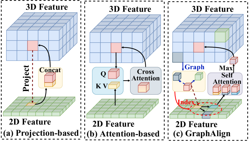
Figure 1: Comparison of feature alignment strategies: (a) Projection-based quickly establishes the relationship between modal features but may suffer from misalignment due to sensor error. (b) Attention-based preserves semantic information by learning alignment but has a high computational cost. (c) Our proposed GraphAlign uses graph-based feature alignment to match more plausible alignments between modalities with reduced computation and improved accuracy.

3D object detection, a vital computer vision task in autonomous driving, relies on deep learning for accurately identifying and locating objects [36, 67, 65, 8, 66, 43, 50, 52] in 3D space [34, 60, 58, 35, 86]. With the availability of diverse sensor data, such as cameras and LiDAR, 3D object detection research has made significant progress. However, challenges and difficulties remain due to the inherent limitations of each modality. While LiDAR point cloud provides accurate depth information, it lacks semantic information. Conversely, camera images contain semantic information but lack depth information [34, 58]. Therefore, multi-modal 3D object detection has been proposed to leverage the complementary advantages of both modalities to improve detection performance.

Despite the potential of multi-modal 3D object detection, the effective fusion of heterogeneous modal features has not been fully explored. In this work, we mainly attribute the current difficulties of training multi-modal detectors to two aspects. On the one hand, many methods [54, 55, 15, 49, 27, 17, 64, 79, 11, 78, 70, 81, 22, 5, 84, 4, 16, 32, 85, 63, 72, 39, 61, 80, 37, 29, 28] rely on establishing deterministic correspondences between points and image pixels to fuse point clouds and image, as shown in Fig. 1 (a). However, accuracy errors resulting from the difference between LiDAR and camera sensors, such as timing synchronization errors, especially the misalignment of small objects in long-range feature fusion, can lead to a decrease in detection performance. On the other hand, a few methods [24, 7, 6, 1] employ attention-based solution to accomplish feature alignment rather than projection, as shown in Fig. 1 (b). However, the key issue with using attention-based for point cloud and image feature alignment in multi-modal 3D object detection is that it is too computationally expensive and cannot meet the real-time detection requirements.

In this work, we propose GraphAlign, a graph matching-based feature alignment strategy, to enhance the accuracy of multi-modal 3D object detection, as shown in Fig. 1 (c). GraphAlign comprises two key modules: Graph Feature Alignment (GFA) and Self-Attention Feature Alignment (SAFA). The GFA module divides the point cloud space into subspaces and generates the K nearest neighbor features for each point cloud. It then transforms the local neighborhood information of the point cloud into image neighborhood information via a projection calibration matrix, followed by one-to-many feature fusion between a single point cloud feature and K neighbor image features. The SAFA module employs a self-attention mechanism to enhance the weights of important relationships in the fused features and selects the most critical feature from K fused features. Our work’s main contributions can be summarized as follows:

• We propose GraphAlign, a feature alignment framework based on graph matching, to address the misalignment issue in multi-modal 3D object detection.

• We propose Graph Feature Alignment (GFA) and Self-Attention Feature Alignment (SAFA) modules to achieve accurate alignment of image features and point cloud features, which can further enhance the feature alignment between point cloud and image modalities, leading to improved detection accuracy.

• Experiments are conducted using the KITTI[12] and nuScenes [2] benchmarks, demonstrating that GraphAlign can boost point cloud detection accuracy, especially for long-range object detection.

Figure 2: The framework of GraphAlign. It consists of the Graph Feature Alignment (GFA) module and the Self-Attention Feature Alignment (SAFA) module. The GFA module takes image and point cloud features as input, uses projection calibration matrix to convert 3D positions to 2D pixel positions, constructs local neighborhood information to find nearest neighbors, and combines image and point cloud features. The SAFA module models the contextual relationships among K nearest neighbors through self-attention mechanism, thereby enhancing the importance of fused features, ultimately selecting the most representative features.

2 Related work

2.1 3D Object Detection with Single Modality

3D object detection is commonly conducted using a single modality, either a camera or a LiDAR sensor. Camera-based 3D detection methods[30, 73, 23, 25, 74, 48, 75, 20, 18, 33] take images as input and output object localization in space. Some methods use a modified 2D object detection framework with a monocular camera to directly regress 3D box parameters from images[48, 20, 18, 33]. However, monocular cameras cannot provide depth information, which has led to other methods that use stereo or multi-view images to generate dense 3D geometric representations for 3D object detection[42, 59]. Although camera-based 3D object detection has made remarkable advancements, its accuracy is not as good as 3D detection methods using LiDAR.

LiDAR-based 3D object detection[68, 9, 71, 19, 46, 69] directly processes irregular point cloud data using methods such as PointNet[40] and PointNet++[41]. Other methods convert point cloud data into regular grids using voxels[83] and pillars[19], which is convenient for feature extraction using 3D or 2D CNN processing[71, 13, 57, 51]. Although LiDAR-based 3D object detection is superior to image-based methods, it has limitations due to the sparse nature of point clouds, the lack of texture features, and semantic information.

2.2 3D Object Detection with Multi-modalities

To address the limitations of each modality, various methods combine the data from the two modalities to improve detection performance. PointPainting [54] proposes to enhance each LiDAR point with the semantic score of the corresponding camera image. PI-RCNN[64] fuse semantic features from the image branch and raw LiDAR point clouds to achieve better performance. Frustum PointNets[39] and Frustum-ConvNet[61] utilize images to generate 2D proposals and then lift them up to 3D space (frustum) to narrow the searching space in point clouds. The Mvx-Net[49] method appends RoI pooling image eigenvectors to dense eigenvectors for each voxel in a LiDAR point cloud. 3D-CVF[79] and EPNet[15] explore alignment strategies on feature maps across different modalities with a learned calibration matrix. However, these methods use projection matrices to align two heterogeneous features, which destroys the image semantic information, affecting performance. Other methods propose a learnable alignment method[24, 7, 6, 1] using the cross-attention mechanism. Although this method effectively preserves the semantic information of the image, the frequent query of image features by the attention mechanism increases computational costs.

3 GraphAlign

In this section, we propose an accurate feature alignment, GraphAlign, which achieves the fusion of point clouds and images by graph matching. We adopt the LiDAR-only detector Voxel RCNN [9] and CenterPoint[77] as the baseline. Fig. 2 shows the network architecture of our GraphAlign, which includes two modules: Graph Feature Alignment (GFA) module and Self-Attention Feature Alignment (SAFA) module. The details of GraphAlign are presented in the following.

3.1 Graph Feature Alignment

Previous works on point cloud and image feature alignment have used projection and attention mechanisms, but these solutions have potential problems. Projection is limited by sensor errors, while attention mechanisms require massive computation. To address these issues, we proposed the Graph Feature Alignment (GFA) module, which constructs neighborhood through graph for more accurate and efficient feature alignment.

The GFA module includes both point cloud and image pipelines, where the fusion of deep features occurs before the 3D Sparse CNN process. Voxel-wise encodor is used to obtain the point cloud features after voxelization. We use the depth features of semantic segmenter DeepLabv3 [3] instead of segmentation scores which contain richer appearance cues and larger perception fields, making them more complementary to point cloud fusion. In the projection stage, we treat point clouds as multi-modal aggregation points because point cloud have depth features more suitable for 3D detection than images. We then project the 3D point cloud onto the image plane, as follow:

$$z_{c}\left[\begin{array}[]{c}u\\ v\\ 1\end{array}\right]=hK\left[\begin{array}[]{ll}R&T\end{array}\right]\left[\begin{array}[]{c}P_{x}\\ P_{y}\\ P_{z}\\ 1\end{array}\right]$$ (1)

where, $P_{x}$, $P_{y}$, $P_{z}$ denote the LiDAR point’s 3D location, $u$, $v$, $z_{c}$ denote the 2D location and the depth of its projection on the image plane, $K$ denotes the camera intrinsic parameter, $R$ and $T$ denote the rotation and the translation of the LiDAR with respect to the camera reference system, and $h$ denotes the scale factor due to down-sampling.

Figure 3: GFA Process Flow. (a) sensor accuracy errors lead to misalignment. (b) GFA builds neighbor relationships through graphs in the point cloud feature. (c) We project the point cloud features onto the image features and obtain the K nearest neighbors of the image features. (d) We perform one-to-many fusion, specifically, by fusing each individual point cloud feature with K neighboring image features to achieve a better alignment.

After feature extraction, we obtain the point cloud depth feature, defined as $\mathbf{F_{P}}\in\mathbb{R}^{N\times C}$, where $N$, $C$ are the number of point cloud, and channel of the global feature map, respectively. And the 3D coordinates of the point cloud are defined as $\mathbf{C_{P}}\in\mathbb{R}^{N\times 3}$ , where 3 is the coordinates of the point cloud, represents $(x,y,z)$. To eliminate the impact of feature misalignment due to point cloud data augmentation before 3D to 2D projection, the point cloud is converted to its raw coordinates by inverse operations, such as removing the flip up and down. $\mathbf{C_{P}}$ transforms image $\mathbf{I}\in\mathbb{R}^{h\times w\times 3}$ into pixel coordinates, defined as $\mathbf{C_{I}}\in\mathbb{R}^{N\times 2}$, where 2 is the coordinates of the image pixels, represents $(x,y)$, after the projection calibration matrix Equation (1). However, since the point cloud is projected onto the image, there exists a small range of image coordinates and an extensive range of point cloud coordinates. We have to remove the coordinates of the image pixels that are out of range after the projection, and the correction rule is $N{}^{\prime}=\left\{n_{1},n_{2},\dots,n_{j}\right|0\leq x\leq w,0\leq y\leq h\}$, and $N{}^{\prime}\leq N$. Thus, we obtain the filtered novel pixel coordinates, defined as $\mathbf{C{}^{\prime}_{I}}\in\mathbb{R}^{N{}^{\prime}\times 2}$.

To obtain the neighborhood information of the point cloud, defined as $\mathbf{K_{P}}\in\mathbb{R}^{N\times K}$, where $N$ and $K$ are the number of point cloud and the number of point cloud neighbors, respectively, we performed a data flow in Algorithm (1) and obtained KP by inputting $\mathbf{C_{P}}$ and some hyperparameters. In addition, to save computational cost during this period, we designed subspaces to accelerate the computation, i.e., searching for nearest neighbors in the subspace instead of the whole space.

Input:

Point cloud coordinates $\mathbf{C_{P}}\in\mathbb{R}^{N\times 3}$.

Hyper-parameters: No. of point cloud neighbors $K=36$.

Hyper-parameters: No. of point clouds in the subspace $N_{P_{sub}}=5000$.

1

2while training do

3       No. of subspaces $N_{sub}=N{\div}N_{P_{sub}}$

4      List: $\mathbf{K_{P}}$

5      for $i_{sub}=1\dots N_{sub}$ do

6             $\mathbf{C_{P}}^{i_{sub}}=[P_{(i_{sub}-1)\times N_{sub}},\dots,P_{N_{sub}\times i_{sub}}]$

7            if $\mathbf{C_{P}}^{i_{sub}}>K$ then

8                   $D_{sub}$ =$[\sqrt{(c_{p}^{2}-c_{p_{i}}^{2})}|c_{p}\in\mathbf{C_{P}}^{i_{sub}},i=1,\dots,N_{P_{sub}}]$

9                  $\mathbf{K_{P_{sub}}}$=Min($D_{sub}$, K)

10                  $\mathbf{K_{P}}=\mathbf{{K_{P}}.Append(\mathbf{K_{P_{sub}}})}$

11            else

12                   $N_{P_{sub}}$=REM(Num(${C_{P}}$))

13                  $D_{sub}$ =$[\sqrt{(c_{p}^{2}-c_{p_{i}}^{2})}|c_{p}\in\mathbf{C_{P}}^{i_{sub}},i=1,\dots,N_{P_{sub}}]$

14                  $\mathbf{K_{P_{sub}}}$=Min($D_{sub}$, $N_{P_{sub}}$) + $[0,...,0]_{K-N_{P_{sub}}}$

15                  $\mathbf{K_{P}}=\mathbf{{K_{P}}.Append(\mathbf{K_{P_{sub}}})}$

16             end if

17            

18       end for

19      

20 end while

21

Output: Point cloud neighbors $\mathbf{K_{P}}\in\mathbb{R}^{N\times K\times C}$.

Algorithm 1 Graph for the point cloud neighbors

In addition, we map the neighbors of the point cloud to the image neighbors, defined as $\mathbf{K_{I}}\in\mathbb{R}^{N\times K}$, where $\mathbf{K_{I}}=\mathbf{K_{P}}$. There are three main reasons why we have not constructed neighbor coordinates for images in this process but mapped by point clouds: First, point cloud coordinates provide richer Euclidean information than images because they are three-dimensional. Second, the graph is designed for input objects with irregular and unstructured data structures like point clouds rather than regular data like images. Third, there is an insurmountable gap between the 3D point cloud coordinates and the 2D image coordinates of two heterogeneous neighborhoods, making it difficult to construct neighbor coordinates for images.

For the above reasons, we choose to index the point cloud neighborhood to the image. Image segmentation encoder outputs image depth features, defined as $\mathbf{F_{I}}\in\mathbb{R}^{h\times w\times c{}^{\prime}}$, which are indexed by $\mathbf{C{}^{\prime}_{I}}$ to obtain novel image depth feature $\mathbf{F{}^{\prime}_{I}}\in\mathbb{R}^{N\times C}$ that are consistent with the point cloud coordinates. Then, indexing the image depth features $\mathbf{F^{\prime}{I}}$ with $\mathbf{K_{I}}$, we obtain the image depth features with neighbors, defined as $\mathbf{F_{K_{I}}}\in\mathbb{R}^{N\times K\times C}$, where $N$, $K$, and $C$ are the number of point cloud, the number of image neighbors, and channel of the point cloud feature map, respectively. We replicate the point cloud depth feature $\mathbf{F_{P}}$ by $K$ times, defined as $\mathbf{F_{K_{P}}}\in\mathbb{R}^{N\times K\times C}$. Instead of fusing point cloud neighbors and image neighbors, we directly perform $K$ replicated point clouds and $K$ image neighbors fusion for the following reasons. Instead of fusing the point cloud neighbors and the image neighbors, we directly perform the fusion of the replicated $K$ times of the point cloud and the image neighbors to find the most appropriate fusion relationship between points and pixels, as shown in Fig. 3. Finally, we obtain the fused features of point clouds and images with neighborhood relations, as follow:

$$\mathbf{F_{K_{PI}}}=\mathbf{F_{K_{P}}}+\mathbf{F_{K_{I}}}$$ (2)

where, $\mathbf{F_{K_{PI}}}\in\mathbb{R}^{N\times K\times C}$ is the fusion feature. $N$, $K$, and $C$ are the number of point cloud, the number of image neighbors, and channel of the point cloud feature map, respectively.

3.2 Self-Attention Feature Alignment

After obtaining the fused features in the GFA module as mentioned above, the aggregation relationship between these features and their K neighbors was found to be underestimated. To overcome this limitation, we introduced the SAFA module as a complementary component to the GFA module. It employs self-attention mechanism to amplify the importance of significant fusion features, as illustrated in Fig. 4.

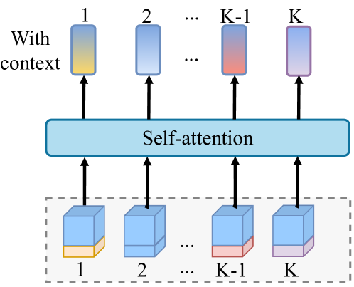
Figure 4: SAFA module flow. The head and max modules are simplified here, and the SAFA module aims to enhance the expression of fusion features by improving the global context information between the K neighborhoods.

Currently, a few methods [7, 6, 1, 24] employ cross-attention to learn the feature alignment of point clouds and image heterogeneous modalities. However, the computational cost is high: given the point number $N$ and the size of image feature $W\times H$, the complexity is $O(NWHC)$. Our SAFA module is based on the GFA module and achieves further vital fusion feature weight assignment by performing a multi-head self-attention operation on $\mathbf{F_{K_{PI}}}$ , and its computation complexity is $O(NK^{2}C)$, where $N$ is the number of point clouds, $K$ as hyperparameters is mostly 36, $w$ and $h$ are the width and height of the image, which are 1272 and 375 pixels in the KITTI[12] dataset, and $C$ is the feature dimension, which is generally 16. By that means, the computation complexity of the cross-attention mechanism-based methods is 400 times higher than our SAFA module.

Specifically, the GFA module outputs fusion features $\mathbf{F_{K_{PI}}}\in\mathbb{R}^{N\times K\times C}$, which we perform a multi-head self-attention operation to find more suitable fusion features with neighborhoods to improve detection performance. As in Algorithm(2), we present a remarkably detailed process flow diagram for the SAFA module, which we perform in a calculation-saving manner, and ultimately output a novel fusion feature,defined as $\mathbf{F_{K_{SAFA}}}\in\mathbb{R}^{N\times K\times C}$, where, $N$, $K$, and $C$ are the number of point cloud, the number of image neighbors, and channel of the point cloud feature map, respectively.

The SAFA module aims to enhance the representation of fusion features by better learning the context global information among the K neighborhoods. Finally, we select the max operation to make up the more significant features for get a novel fusion feature, defined as $\mathbf{F_{m_{PI}}}\in\mathbb{R}^{N\times C}$, as follow:

$$\mathbf{F_{m_{PI}}}=Max(\mathbf{F_{K_{SAFA}}})$$ (3)

where, $N$, $C$ are the number of point cloud, channel of the point cloud feature map, respectively.

Input:

The GFA module outputs fusion features: $\mathbf{F_{K_{PI}}}\in\mathbb{R}^{N\times K\times C}$

Hyper-parameters: No. of attention heads $H$=1.

Output: A noval fusion feature with attention: $\mathbf{F_{K_{SAFA}}}\in\mathbb{R}^{N\times K\times C}$.

1 while training do

2      

3      $W_{\emph{q}},W_{\emph{k}},W_{\emph{v}}\in\mathbb{R}^{C\times C}$

4      

5      $Q,K,V=[W_{\emph{q}},W_{\emph{k}},W_{\emph{v}}]\mathbf{F_{K_{PI}}}$ 

6      Add $H$ by Reshape:     $Q,K,V\in\mathbb{R}^{N\times K\times C}$ $->\mathbb{R}^{N\times H\times K\times\frac{C}{H}}$

7      

8      $Att=Softmax(QK),Att\in\mathbb{R}^{N\times H\times K\times\frac{C}{H}}$

9      $\mathbf{F_{K_{SAFA}}}=Att\mathbf{F_{K_{PI}}}$, $\mathbf{F_{K_{SAFA}}}\in\mathbb{R}^{N\times K\times C}$

10 end while

Algorithm 2 SAFA module workflow

3.3 LiDAR Detection

Generally, images serve as auxiliary features for point clouds. After the fusion of point cloud and image, $\mathbf{F_{m_{PI}}}$ is fed into the subsequent LiDAR pipeline for further detection. Our fusion process is completed during the 3D backbone of the LiDAR pipeline, as shown in Fig. 2. Subsequently, we transform 3D features into BEV features and finally predict using the detection head. In addition, the predicted 3D box of the point cloud can be converted into the 2D box of the image using the projection matrix.

4 Experiments

In this section, we present the details of each dataset and the experimental setup of GraphAlign, and evaluate the performance of 3D object detection on KITTI[12] and nuScenes[2] datasets.

4.1 Dataset and Evaluation Metrics

4.1.1 KITTI dataset

The KITTI dataset [12] provides synchronized LiDAR point clouds and front-view camera images, and consists of 7,481 training samples and 7,518 test samples. The standard evaluation metric for object detection is mean Average Precision (mAP), computed using recall at 40 positions (R40). In this work, we evaluate our models on the most commonly used car category using Average Precision (AP) with an Intersection over Union (IoU) threshold of 0.7. To compare our results with other state-of-the-art methods on the KITTI 3D detection benchmark, we split the KITTI training dataset into a 4:1 ratio for training and validation, and report our performance on the KITTI test dataset.

4.1.2 nuScenes dataset

The nuScenes dataset [2] is a large-scale 3D detection benchmark consisting of 700 training scenes, 150 validation scenes, and 150 testing scenes. The data were collected using six multi-view cameras and a 32-channel LiDAR sensor, and the dataset includes 360-degree object annotations for 10 object classes. To evaluate the detection performance, the primary metrics used are the mean Average Precision (mAP) and the nuScenes detection score (NDS), which assess a method’s detection accuracy in terms of classification, bounding box location, size, orientation, attributes, and velocity.

Table 1: Performance comparison with the state-of-the-art methods on KITTI test set for car 3D detection with an average precision of 40 sampling recall points evaluated on KITTI server. ‘L’ and ‘C’ represent LiDAR and Camera, respectively.

Method	Modality	AP${}_{3D}(\%)$			AP${}_{BEV}(\%)$
		Easy	Mod.	Hard	Easy	Mod.	Hard
PV-RCNN [45]	L	90.25	81.43	76.82	94.98	90.65	86.14
SECOND [71]	L	84.65	75.96	68.71	88.07	79.37	77.50
PointPillars [19]	L	82.58	74.31	68.99	90.07	86.56	82.81
VoxSet [13]	L	88.53	82.06	77.46	-	-	-
TANet [31]	L	84.39	75.94	68.82	91.58	86.54	81.19
Part-A2 [47]	L	85.94	77.86	72.00	89.52	84.76	81.47
VP-Net [51]	L	90.46	82.03	79.65	94.49	90.99	86.58
MV3D [4]	L&C	74.97	63.63	54.00	86.62	78.93	69.80
MMF [26]	L&C	86.81	76.75	68.41	89.49	87.47	79.10
PI-RCNN [64]	L&C	84.37	74.82	70.03	91.44	85.81	81.00
EPNet [15]	L&C	89.81	79.28	74.59	94.22	88.47	83.69
PointPainting [54]	L&C	82.11	71.70	67.08	-	-	-
MSF-MC [62]	L&C	89.63	80.06	75.83	93.42	86.97	84.54
Fast-CLOCs [38]	L&C	89.11	80.34	76.98	93.02	89.49	86.39
Focals Conv [5]	L&C	90.55	82.28	77.59	-	-	-
SFD [63]	L&C	91.73	84.76	77.92	95.64	91.85	86.83
HMFI [21]	L&C	88.90	81.93	77.30	-	-	-
Graph-VoI [72]	L&C	91.89	83.27	77.78	95.69	90.10	86.85
Voxcl RCNN [9]	L	90.90	81.62	77.06	-	-	-
Voxcl RCNN*	L	90.76	81.69	77.42	92.89	89.97	84.69
blue!10 Our GraphAlign	L&C	90.96	83.49	80.14	93.91	91.79	88.05

• * denotes re-implement result.

4.2 Implementation Details

4.2.1 Network Architecture

Since KITTI [12] and nuScenes [2] are distinct datasets with varying evaluation metrics and characteristics, we provide a detailed description of the GraphAlign settings for each dataset in the following section.

GraphAlign with Voxel RCNN [9]: We validate our GraphAlign on the KITTI [12] dataset using Voxel RCNN [9] as the baseline. The input voxel size is set to (0.05m, 0.05m, 0.1m), with anchor sizes for cars set at [3.9, 1.6, 1.56], and anchor rotations at [0, 1.57]. We adopt the same data augmentation solution as Focal Loss [5].

GraphAlign with CenterPoint [77]: We validate our GraphAlign on the nuScenes [2] dataset using CenterPoint [77] as the baseline. The detection range for the X and Y axis is set at [-54m, 54m] and [-5m, 3m] for the Z axis. The input voxel size is set at (0.075m, 0.075m, 0.2m), and the maximum number of point clouds contained in each voxel is set to 10.

Table 2: Performance comparison with state-of-the-art methods on KITTI validation dataset for car class. The results are reported by the mAP with 0.7 IoU threshold and 40 recall points. ‘L’ and ‘C’ represent LiDAR and Camera, respectively.

Method	Moiality	AP${}_{3D}(\%)$			AP${}_{BEV}(\%)$
		Easy	Mod.	Hard	Easy	Mod.	Hard
PointRCNN [46]	L	88.88	78.63	77.38	_	_	_
SECOND [71]	L	87.43	76.48	69.10	_	_	_
CT3D [44]	L	92.85	85.82	83.46	96.14	91.88	89.63
Part-A2 [47]	L	89.47	79.47	78.54	90.42	88.61	87.31
MV3D [4]	L&C	71.29	62.68	56.56	86.55	78.10	76.67
MMF [26]	L&C	87.90	77.87	75.57	96.66	88.25	79.60
MSF-MC [62]	L&C	89.63	80.06	75.83	93.42	86.97	84.54
PI-RCNN [64]	L&C	88.27	78.53	77.75	_	_	_
EPNet [15]	L&C	92.28	82.59	80.14	95.51	91.47	91.16
Voxel RCNN [9]	L	92.38	85.29	82.86	95.52	91.25	88.99
blue!10 Our GraphAlign	L&C	92.44	87.01	84.68	95.65	92.82	91.41

4.2.2 Training and Testing Details

Our GraphAlign is meticulously trained from scratch using the Adam optimizer and incorporates a stand-alone semantic segmenter, namely, DeepLabv3 [3]. To enable effective training on KITTI [12] and nuScenes [2], we utilize 8 NVIDIA RTX A6000 GPUs for network training. Specifically, for KITTI, our GraphAlign model based on Voxel RCNN [9] requires approximately 2 hours of training time which train 80 epochs. Whereas for nuScenes, our GraphAlign model based on CenterPoint [77] necessitates approximately 20 hours of training time which train 20epochs. During the model inference stage, we employ a non-maximal suppression (NMS) operation in RPN with an IoU threshold of 0.7 and select the top 100 region proposals to serve as input for the detection head. Following refinement, we apply NMS again with an IoU threshold of 0.1 to eliminate redundant predictions. For additional details concerning our method, please refer to OpenPCDet [53].

4.3 Comparison with State-of-the-Arts

Table 3: Comparison with SOTA methods on the nuScenes test set. ‘C.V.’, ‘Ped.’, and ‘T.C.’ are short for construction vehicle, pedestrian, and traffic cone, respectively.

Method	mAP	NDS	Car	Truck	C.V.	Bus	Trailer	Barrier	Motor.	Bike	Ped.	T.C.
InfoFocus [56]	39.5	39.5	77.9	31.4	10.7	44.8	37.3	47.8	29.0	6.1	63.4	46.5
S2M2-SSD [82]	62.9	69.3	86.3	56.0	26.2	65.4	59.8	75.1	61.6	36.4	84.6	77.7
AFDetV2 [14]	62.4	68.5	86.3	54.2	26.7	62.5	58.9	71.0	63.8	34.3	85.8	80.1
VISTA [10]	63.0	69.8	84.4	55.1	25.1	63.7	54.2	71.4	70.0	45.4	82.8	78.5
PointPillars[19]	30.5	45.3	68.4	23.0	4.1	28.2	23.4	38.9	27.4	1.1	59.7	30.8
PointPainting [54]	46.4	58.1	77.9	35.8	15.8	36.2	37.3	60.2	41.5	24.1	73.3	62.4
MVP [78]	66.4	70.5	86.8	58.5	26.1	67.4	57.3	74.8	70.0	49.3	89.1	85.0
AutoAlign[7]	65.8	70.9	85.9	55.3	29.6	67.7	55.6	-	71.5	51.5	86.4	-
AutoAlignV2[6]	68.4	72.4	87.0	59.0	33.1	69.3	59.3	-	72.9	52.1	87.6	-
TransFusion [1]	68.9	71.7	87.1	60.0	33.1	68.3	60.8	78.1	73.6	52.9	88.4	86.7
BEVFusion [28]	69.2	71.8	88.1	60.9	34.4	69.3	62.1	78.2	72.2	52.2	89.2	85.2
DeepInteraction [76]	70.8	73.4	87.9	60.2	37.5	70.8	63.8	80.4	75.4	54.5	90.3	87.0
CenterPoint [77]	58.0	65.5	84.6	51.0	17.5	60.2	53.2	70.9	53.7	28.7	83.4	76.7
blue!10 Our GraphAlign	66.5+8.5	70.6+5.1	87.6	57.7	26.1+8.6	66.2	57.8	74.1	72.5+18.8	49.0+20.3	87.2	86.3+9.6

Table 4: Effect of each component in our GraphAlign. Results are reported on KITTI validation set with Voxel RCNN. ”P” indicates projection.

P	GFA	SAFA	AP${}_{3D}(\%)$		#Params	Runtime
			Mod.	Hard
			85.29	82.86	7.59 M	5ms
✓			85.59+0.30	83.07+0.21	7.74 M	17ms
✓	✓		86.62+1.03	84.21+1.14	7.74 M	24ms
blue!10 ✓	✓	✓	87.01+0.39	84.68+0.47	7.75 M	26ms

4.3.1 Performance on KITTI dataset.

As shown in Table 1 , we compare GraphAlign with state-of-the-art methods in 3D and BEV APs on KITTI test dataset. We observe that our GraphAlign achieves state-of-the-art performance. In detail, it shows remarkably outstanding performance at three difficulty levels of 3D and BEV detection, with (90.96%, 83.49%, 80.14%, 93.91%, 91.79%, 88.05%). For better comparison, we reproduce Voxel RCNN [9] as a strong baseline network. It is worth noting that our replication is almost identical to the results reported in [9]. Our GraphAlign achieves better performance than the baseline Voxel RCNN with (0.06%, 1.80%, 2.72%, 1.02%, 1.82%, 3.36%) improvements on three levels. Compared with the multi-modal method Focals Conv [5], our GraphAlign achieves better performance than Focals Conv with the improvements (0.41%, 1.21%, 2.72%). Our GraphAlign performs well on the KITTI [12] test dataset’s moderate and hard levels, which have more long-range objects. In addition, we also provide the results of the KITTI validation dataset to better present the detection performance of our GraphAlign, as shown in Table 2. There is a significant improvement compared to the baseline Voxel RCNN on the KITTI [12] validation dataset’s moderate and hard levels. Even slight misalignments between point clouds and images can likely lead to significant errors in detection. GraphAlign’s ability to use graphs to establish relationships between heterogeneous modalities is a key factor in its success.

4.3.2 Performance on nuScenes dataset.

We also conducted experiments on the much larger nuScenes [2] dataset using the state-of-the-art 3D detector CenterPoint [77] to further validate the effectiveness of our GraphAlign. As shown in Table 3, GraphAlign achieved 66.5 mAP and 70.6 NDS on the nuScenes test dataset, which is 8.5 mAP and 5.1 NDS higher than the strong CenterPoint[77]. Furthermore, we marked in red those categories, ”C.V.,” ”Motor,” ”Bike,” and ”T.C.,” that showed a significant increase in performance, with ”Motor” and ”Bike” increasing by 18.8% and 20.3%, respectively. Our GraphAlign exhibits excellent performance in small object detection, particularly for these four categories that are characterized by a higher proportion of small objects at long distances, following more accurate feature alignment.

Table 5: Effect of each component in our GraphAlign. Results are reported on nuScenes $\frac{1}{4}$ validation with CenterPoint. ”P” indicates projection.

P	GFA	SAFA	mAP	NDS	#Params	Runtime
			56.1	64.2	9.01M	12ms
✓			58.0+1.9	64.8+0.6	9.16M	28ms
✓	✓		61.3+3.3	67.8+3.0	9.16M	35ms
blue!10 ✓	✓	✓	62.8+1.5	68.5+0.7	9.17M	37ms

• * denotes re-implement result.

4.4 Ablation Study

4.4.1 Effect of Projection-only, the GFA and SAFA modules, and Attention-based

This section discusses the results of ablation experiments conducted on the baseline detectors Voxel RCNN and CenterPoint to evaluate the performance of each module in GraphAlign. The results are reported in Table 4 and Table 5 for KITTI and nuScenes $\frac{1}{4}$ validation datasets, respectively.

As shown in Table 4, the moderate and hard AP scores for KITTI are initially at 85.29% and 82.86%, respectively. Adding the projection-only module to the image branch only slightly improves the mAP score by 0.30% and 0.21%, respectively. The lackluster performance was due to the intrinsic misalignment caused by the sensors’ accuracy errors. However, compared with projection-only, the consecutive addition of GFA and SAFA modules led to a continuous improvement of AP on the moderate and hard levels of KITTI, by 1.03% and 0.39% (moderate) and 1.14% and 0.47% (hard), respectively. This significant performance improvement is attributed to our GraphAlign method’s accurate alignment of long-range objects.

As shown in Table 5, the Attention-based feature alignment strategy AutoAlignV2[6] shows slightly improved detection accuracy compared to GraphAlign, its runtime is five times longer and cannot meet the real-time requirement. The reason for this is the global alignment learning between the point cloud and the image through the Attention mechanism, while our GraphAlign learns local relationships based on projection, similar to the Anchor mechanism, to enable faster learning based on prior knowledge. Although the SAFA module with an attention mechanism has been added to our GraphAlign, it focuses on learning important local features of neighbors rather than computing with global image features.

4.4.2 Effect of the Hyperparameters

In this section, we have analyzed the experimental results of our model with respect to various hyperparameters, including $K$ (number of point cloud neighbors), $N_{P_{sub}}$ (number of point clouds in the subspace), and $H$ (number of attention heads) for the car class on the KITTI validation dataset and $\frac{1}{4}$ on nuScenes.

Table 6 indicates that the optimal performance for GraphAlign based on Voxel RCNN was achieved when $K$ was set to 16, while for GraphAlign based on CenterPoint, the optimal value was 25. Although there was a slight improvement in performance on easy and moderate levels for $K$ set to 25 and 36, respectively, the corresponding increase in computation time by 11

Moreover, Table 7 reveals that the runtime was significantly impacted by $N_{P_{sub}}$. We found that the best performance was achieved with $N_{P_{sub}}$ set to 1000. Even though setting $N_{P_{sub}}$ to 3000 resulted in a slight improvement in accuracy on the KITTI dataset, the increase in AP was limited, and the runtime increased by 38%. Therefore, we selected 1000 as the optimal value for $N_{P_{sub}}$. Subdividing the subspace proved critical in saving time, and setting $N_{P_{sub}}$ to 500 did not improve performance.

Additionally, as depicted in Fig. 8, as $H$ increases, AP gradually improves, but the effect on runtime is more significant, with an increase of approximately 10%. Generally, $H=1$ is preferred, but larger values may be used to achieve higher AP.

Table 6: Effect of the number of point cloud neighbors $K$.

$K$	KITTI [12]				nuScenes [2]
	AP3D(%)			Runtime	mAP	NDS	Runtime
	Easy	Mod.	Hard
9	91.53	86.38	84.17	25ms	61.9	67.9	35ms
16	92.44	87.01	84.68	26ms	62.1	67.8	37ms
25	92.09	87.11	84.23	29ms	62.8	68.5	41ms
36	92.58	86.87	83.97	34ms	62.9	68.3	47ms
48	92.43	87.58	83.90	40ms	63.1	68.1	54ms

Table 7: Effect of the number of point cloud $N_{P_{sub}}$ in the subspace.

$N_{P_{sub}}$	KITTI [12]				nuScenes [2]
	AP3D(%)			Runtime	mAP	NDS	Runtime
	Easy	Mod.	Hard
500	92.09	86.59	84.01	23ms	60.9	68.8	34ms
1000	92.44	87.01	84.68	26ms	62.8	68.5	37ms
3000	92.57	87.05	84.77	36ms	61.9	68.7	50ms
5000	92.09	86.81	84.12	45ms	62.2	67.9	58ms
8000	91.97	86.24	85.02	53ms	61.8	67.5	69ms
10000	92.11	86.27	84.32	59ms	61.5	67.0	76ms

Table 8: Effect of the number of attention heads $H$.

$H$	KITTI [12]				nuScenes [2]
	AP3D(%)			Runtime	mAP	NDS	Runtime
	Easy	Mod.	Hard
1	92.44	87.01	84.68	26ms	62.8	68.5	37ms
2	93.57	87.89	84.79	29ms	62.9	68.4	41ms
3	92.87	87.69	84.55	35ms	63.1	68.4	47ms
4	93.51	88.13	84.97	41ms	63.5	68.8	56ms

Table 9: Performance on different distances. The results are evaluated with 3D AP calculated by 40 recall positions for car class on the moderate level.

P	GFA	SAFA	AP${}_{3D}(\%)$			AP${}_{BEV}(\%)$
			0-20m	20-40m	40m-inf	0-20m	20-40m	40m-inf
			95.94	79.45	39.45	96.09	89.34	54.00
✓			95.97	79.52+0.07	38.93-0.52	96.48	90.68+1.34	53.54-0.46
✓	✓		96.13	82.02+2.50	46.49+7.56	96.47	92.65+1.88	58.56+5.20
blue!10 ✓	✓	✓	96.12	82.17+0.15	47.67+1.18	96.57	93.54+0.89	59.99+1.43

4.4.3 Distances Analysis

To better understand the excellent performance of our GraphAlign at long distances, we present performance metrics for different distance ranges in Table 9. Specifically, there was a significant drop in Projection-only, particularly in the 40m-inf range where there were many small objects. This was mainly due to misalignment of small objects from different modalities. By adding the GFA and SAFA modules, the 3D APs increased by 7.56% and 1.18% respectively, while the BEV APs increased by 5.20% and 1.43% respectively in the 40m-inf range. These results demonstrated that our GraphAlign’s effective feature alignment strategy is helpful for the long-range small objects detection.

5 Conclusions

In this work,we present GraphAlign, a more accurate and efficient feature alignment strategy for 3D object detection by graph matching. Specifically, the Graph Feature Alignment (GFA) module constructs neighbor fusion features based on prior knowledge of projection matrix, which avoids sensor accuracy errors. Furthermore, the Self-Attention Feature Alignment (SAFA) module is designed to enhance the weight of important relationships. Comprehensive experimental results demonstrate that GraphAlign significantly improves the 3D detector on the KITTI and nuScenes datasets. Building upon existing Projection-based and Attention-based feature alignment strategies, we hope that our work can provide a new perspective for multi-modal feature fusion in autonomous driving.

Limitation and future work. One of our limitations is that our GraphAlign rely on independent semantic segmentation rather than end-to-end learning. As such, in future work, we aim to investigate the use of end-to-end learning for graph matching in multi-modal fusion.

References

- [1] Xuyang Bai, Zeyu Hu, Xinge Zhu, Qingqiu Huang, Yilun Chen, Hongbo Fu, and Chiew-Lan Tai. Transfusion: Robust lidar-camera fusion for 3d object detection with transformers. In Proceedings of the IEEE/CVF Conference on Computer Vision and Pattern Recognition, pages 1090–1099, 2022.
- [2] Holger Caesar, Varun Bankiti, Alex H Lang, Sourabh Vora, Venice Erin Liong, Qiang Xu, Anush Krishnan, Yu Pan, Giancarlo Baldan, and Oscar Beijbom. nuscenes: A multimodal dataset for autonomous driving. In Proceedings of the IEEE/CVF conference on computer vision and pattern recognition, pages 11621–11631, 2020.
- [3] Liang-Chieh Chen, George Papandreou, Florian Schroff, and Hartwig Adam. Rethinking atrous convolution for semantic image segmentation. arXiv preprint arXiv:1706.05587, 2017.
- [4] Xiaozhi Chen, Huimin Ma, Ji Wan, Bo Li, and Tian Xia. Multi-view 3d object detection network for autonomous driving. In Proceedings of the IEEE conference on Computer Vision and Pattern Recognition, pages 1907–1915, 2017.
- [5] Yukang Chen, Yanwei Li, Xiangyu Zhang, Jian Sun, and Jiaya Jia. Focal sparse convolutional networks for 3d object detection. In Proceedings of the IEEE/CVF Conference on Computer Vision and Pattern Recognition, pages 5428–5437, 2022.
- [6] Zehui Chen, Zhenyu Li, Shiquan Zhang, Liangji Fang, Qinhong Jiang, and Feng Zhao. Deformable feature aggregation for dynamic multi-modal 3d object detection. In Computer Vision–ECCV 2022: 17th European Conference, Tel Aviv, Israel, October 23–27, 2022, Proceedings, Part VIII, pages 628–644. Springer, 2022.
- [7] Zehui Chen, Zhenyu Li, Shiquan Zhang, Liangji Fang, Qinghong Jiang, Feng Zhao, Bolei Zhou, and Hang Zhao. Autoalign: Pixel-instance feature aggregation for multi-modal 3d object detection. arXiv preprint arXiv:2201.06493, 2022.
- [8] Kun Dai, Tao Xie, Ke Wang, Zhiqiang Jiang, Dedong Liu, Ruifeng Li, and Jiahe Wang. Eaainet: An element-wise attention network with global affinity information for accurate indoor visual localization. IEEE Robotics and Automation Letters, 8(6):3166–3173, 2023.
- [9] Jiajun Deng, Shaoshuai Shi, Peiwei Li, Wengang Zhou, Yanyong Zhang, and Houqiang Li. Voxel r-cnn: Towards high performance voxel-based 3d object detection. In Proceedings of the AAAI Conference on Artificial Intelligence, volume 35, pages 1201–1209, 2021.
- [10] Shengheng Deng, Zhihao Liang, Lin Sun, and Kui Jia. Vista: Boosting 3d object detection via dual cross-view spatial attention. In Proceedings of the IEEE/CVF Conference on Computer Vision and Pattern Recognition, pages 8448–8457, 2022.
- [11] Jian Dou, Jianru Xue, and Jianwu Fang. Seg-voxelnet for 3d vehicle detection from rgb and lidar data. In 2019 International Conference on Robotics and Automation (ICRA), pages 4362–4368. IEEE, 2019.
- [12] Andreas Geiger, Philip Lenz, and Raquel Urtasun. Are we ready for autonomous driving? the kitti vision benchmark suite. In 2012 IEEE conference on computer vision and pattern recognition, pages 3354–3361. IEEE, 2012.
- [13] Chenhang He, Ruihuang Li, Shuai Li, and Lei Zhang. Voxel set transformer: A set-to-set approach to 3d object detection from point clouds. In Proceedings of the IEEE/CVF Conference on Computer Vision and Pattern Recognition, pages 8417–8427, 2022.
- [14] Yihan Hu, Zhuangzhuang Ding, Runzhou Ge, Wenxin Shao, Li Huang, Kun Li, and Qiang Liu. Afdetv2: Rethinking the necessity of the second stage for object detection from point clouds. In Proceedings of the AAAI Conference on Artificial Intelligence, volume 36, pages 969–979, 2022.
- [15] Tengteng Huang, Zhe Liu, Xiwu Chen, and Xiang Bai. Epnet: Enhancing point features with image semantics for 3d object detection. In European Conference on Computer Vision, pages 35–52. Springer, 2020.
- [16] Jason Ku, Melissa Mozifian, Jungwook Lee, Ali Harakeh, and Steven L Waslander. Joint 3d proposal generation and object detection from view aggregation. In 2018 IEEE/RSJ International Conference on Intelligent Robots and Systems (IROS), pages 1–8. IEEE, 2018.
- [17] Jason Ku, Alex D Pon, Sean Walsh, and Steven L Waslander. Improving 3d object detection for pedestrians with virtual multi-view synthesis orientation estimation. In 2019 IEEE/RSJ International Conference on Intelligent Robots and Systems (IROS), pages 3459–3466. IEEE, 2019.
- [18] Abhinav Kumar, Garrick Brazil, and Xiaoming Liu. Groomed-nms: Grouped mathematically differentiable nms for monocular 3d object detection. In Proceedings of the IEEE/CVF Conference on Computer Vision and Pattern Recognition, pages 8973–8983, 2021.
- [19] Alex H Lang, Sourabh Vora, Holger Caesar, Lubing Zhou, Jiong Yang, and Oscar Beijbom. Pointpillars: Fast encoders for object detection from point clouds. In Proceedings of the IEEE/CVF conference on computer vision and pattern recognition, pages 12697–12705, 2019.
- [20] Peixuan Li, Huaici Zhao, Pengfei Liu, and Feidao Cao. Rtm3d: Real-time monocular 3d detection from object keypoints for autonomous driving. In European Conference on Computer Vision, pages 644–660. Springer, 2020.
- [21] Xin Li, Botian Shi, Yuenan Hou, Xingjiao Wu, Tianlong Ma, Yikang Li, and Liang He. Homogeneous multi-modal feature fusion and interaction for 3d object detection. In European Conference on Computer Vision, pages 691–707. Springer, 2022.
- [22] Yanwei Li, Yilun Chen, Xiaojuan Qi, Zeming Li, Jian Sun, and Jiaya Jia. Unifying voxel-based representation with transformer for 3d object detection. arXiv preprint arXiv:2206.00630, 2022.
- [23] Yinhao Li, Zheng Ge, Guanyi Yu, Jinrong Yang, Zengran Wang, Yukang Shi, Jianjian Sun, and Zeming Li. Bevdepth: Acquisition of reliable depth for multi-view 3d object detection. In Proceedings of the AAAI Conference on Artificial Intelligence, volume 37, pages 1477–1485, 2023.
- [24] Yingwei Li, Adams Wei Yu, Tianjian Meng, Ben Caine, Jiquan Ngiam, Daiyi Peng, Junyang Shen, Yifeng Lu, Denny Zhou, Quoc V Le, et al. Deepfusion: Lidar-camera deep fusion for multi-modal 3d object detection. In Proceedings of the IEEE/CVF Conference on Computer Vision and Pattern Recognition, pages 17182–17191, 2022.
- [25] Zhiqi Li, Wenhai Wang, Hongyang Li, Enze Xie, Chonghao Sima, Tong Lu, Yu Qiao, and Jifeng Dai. Bevformer: Learning bird’s-eye-view representation from multi-camera images via spatiotemporal transformers. In European conference on computer vision, pages 1–18. Springer, 2022.
- [26] Ming Liang, Bin Yang, Yun Chen, Rui Hu, and Raquel Urtasun. Multi-task multi-sensor fusion for 3d object detection. In Proceedings of the IEEE/CVF Conference on Computer Vision and Pattern Recognition, pages 7345–7353, 2019.
- [27] Ming Liang, Bin Yang, Shenlong Wang, and Raquel Urtasun. Deep continuous fusion for multi-sensor 3d object detection. In Proceedings of the European conference on computer vision (ECCV), pages 641–656, 2018.
- [28] Tingting Liang, Hongwei Xie, Kaicheng Yu, Zhongyu Xia, Zhiwei Lin, Yongtao Wang, Tao Tang, Bing Wang, and Zhi Tang. Bevfusion: A simple and robust lidar-camera fusion framework. arXiv preprint arXiv:2205.13790, 2022.
- [29] Zhijian Liu, Haotian Tang, Alexander Amini, Xinyu Yang, Huizi Mao, Daniela Rus, and Song Han. Bevfusion: Multi-task multi-sensor fusion with unified bird’s-eye view representation. arXiv preprint arXiv:2205.13542, 2022.
- [30] Zechen Liu, Zizhang Wu, and Roland Tóth. Smoke: Single-stage monocular 3d object detection via keypoint estimation. In Proceedings of the IEEE/CVF Conference on Computer Vision and Pattern Recognition Workshops, pages 996–997, 2020.
- [31] Zhe Liu, Xin Zhao, Tengteng Huang, Ruolan Hu, Yu Zhou, and Xiang Bai. Tanet: Robust 3d object detection from point clouds with triple attention. In Proceedings of the AAAI Conference on Artificial Intelligence, volume 34, pages 11677–11684, 2020.
- [32] Haihua Lu, Xuesong Chen, Guiying Zhang, Qiuhao Zhou, Yanbo Ma, and Yong Zhao. Scanet: Spatial-channel attention network for 3d object detection. In ICASSP 2019-2019 IEEE International Conference on Acoustics, Speech and Signal Processing (ICASSP), pages 1992–1996. IEEE, 2019.
- [33] Shujie Luo, Hang Dai, Ling Shao, and Yong Ding. M3dssd: Monocular 3d single stage object detector. In Proceedings of the IEEE/CVF Conference on Computer Vision and Pattern Recognition, pages 6145–6154, 2021.
- [34] Jiageng Mao, Shaoshuai Shi, Xiaogang Wang, and Hongsheng Li. 3d object detection for autonomous driving: A review and new outlooks. arXiv preprint arXiv:2206.09474, 2022.
- [35] Jiageng Mao, Shaoshuai Shi, Xiaogang Wang, and Hongsheng Li. 3d object detection for autonomous driving: A comprehensive survey. International Journal of Computer Vision, pages 1–55, 2023.
- [36] Arthur Moreau, Thomas Gilles, Nathan Piasco, Dzmitry Tsishkou, Bogdan Stanciulescu, and Arnaud de La Fortelle. Imposing: Implicit pose encoding for efficient visual localization. In Proceedings of the IEEE/CVF Winter Conference on Applications of Computer Vision, pages 2892–2902, 2023.
- [37] Anshul Paigwar, David Sierra-Gonzalez, Özgür Erkent, and Christian Laugier. Frustum-pointpillars: A multi-stage approach for 3d object detection using rgb camera and lidar. In Proceedings of the IEEE/CVF International Conference on Computer Vision, pages 2926–2933, 2021.
- [38] Su Pang, Daniel Morris, and Hayder Radha. Fast-clocs: Fast camera-lidar object candidates fusion for 3d object detection. In Proceedings of the IEEE/CVF Winter Conference on Applications of Computer Vision, pages 187–196, 2022.
- [39] Charles R Qi, Wei Liu, Chenxia Wu, Hao Su, and Leonidas J Guibas. Frustum pointnets for 3d object detection from rgb-d data. In Proceedings of the IEEE conference on computer vision and pattern recognition, pages 918–927, 2018.
- [40] Charles R Qi, Hao Su, Kaichun Mo, and Leonidas J Guibas. Pointnet: Deep learning on point sets for 3d classification and segmentation. In Proceedings of the IEEE conference on computer vision and pattern recognition, pages 652–660, 2017.
- [41] Charles Ruizhongtai Qi, Li Yi, Hao Su, and Leonidas J Guibas. Pointnet++: Deep hierarchical feature learning on point sets in a metric space. Advances in neural information processing systems, 30, 2017.
- [42] Danila Rukhovich, Anna Vorontsova, and Anton Konushin. Imvoxelnet: Image to voxels projection for monocular and multi-view general-purpose 3d object detection. In Proceedings of the IEEE/CVF Winter Conference on Applications of Computer Vision, pages 2397–2406, 2022.
- [43] Paul-Edouard Sarlin, Daniel DeTone, Tsun-Yi Yang, Armen Avetisyan, Julian Straub, Tomasz Malisiewicz, Samuel Rota Bulò, Richard Newcombe, Peter Kontschieder, and Vasileios Balntas. Orienternet: Visual localization in 2d public maps with neural matching. In Proceedings of the IEEE/CVF Conference on Computer Vision and Pattern Recognition, pages 21632–21642, 2023.
- [44] Hualian Sheng, Sijia Cai, Yuan Liu, Bing Deng, Jianqiang Huang, Xian-Sheng Hua, and Min-Jian Zhao. Improving 3d object detection with channel-wise transformer. In Proceedings of the IEEE/CVF International Conference on Computer Vision, pages 2743–2752, 2021.
- [45] Shaoshuai Shi, Chaoxu Guo, Li Jiang, Zhe Wang, Jianping Shi, Xiaogang Wang, and Hongsheng Li. Pv-rcnn: Point-voxel feature set abstraction for 3d object detection. In Proceedings of the IEEE/CVF Conference on Computer Vision and Pattern Recognition, pages 10529–10538, 2020.
- [46] Shaoshuai Shi, Xiaogang Wang, and Hongsheng Li. Pointrcnn: 3d object proposal generation and detection from point cloud. In Proceedings of the IEEE/CVF conference on computer vision and pattern recognition, pages 770–779, 2019.
- [47] Shaoshuai Shi, Zhe Wang, Jianping Shi, Xiaogang Wang, and Hongsheng Li. From points to parts: 3d object detection from point cloud with part-aware and part-aggregation network. IEEE transactions on pattern analysis and machine intelligence, 43(8):2647–2664, 2020.
- [48] Andrea Simonelli, Samuel Rota Bulo, Lorenzo Porzi, Manuel López-Antequera, and Peter Kontschieder. Disentangling monocular 3d object detection. In Proceedings of the IEEE/CVF International Conference on Computer Vision, pages 1991–1999, 2019.
- [49] Vishwanath A Sindagi, Yin Zhou, and Oncel Tuzel. Mvx-net: Multimodal voxelnet for 3d object detection. In 2019 International Conference on Robotics and Automation (ICRA), pages 7276–7282. IEEE, 2019.
- [50] Ziying Song, Li Wang, Guoxin Zhang, Caiyan Jia, Jiangfeng Bi, Haiyue Wei, Yongchao Xia, Chao Zhang, and Lijun Zhao. Fast detection of multi-direction remote sensing ship object based on scale space pyramid. In 2022 18th International Conference on Mobility, Sensing and Networking (MSN), pages 1019–1024. IEEE, 2022.
- [51] Ziying Song, Haiyue Wei, Caiyan Jia, Yongchao Xia, Xiaokun Li, and Chao Zhang. Vp-net: Voxels as points for 3d object detection. IEEE Transactions on Geoscience and Remote Sensing, 2023.
- [52] Ziying Song, Yu Zhang, Yi Liu, Kuihe Yang, and Meiling Sun. Msfyolo: Feature fusion-based detection for small objects. IEEE Latin America Transactions, 20(5):823–830, 2022.
- [53] OD Team et al. Openpcdet: An open-source toolbox for 3d object detection from point clouds, 2020.
- [54] Sourabh Vora, Alex H Lang, Bassam Helou, and Oscar Beijbom. Pointpainting: Sequential fusion for 3d object detection. In Proceedings of the IEEE/CVF conference on computer vision and pattern recognition, pages 4604–4612, 2020.
- [55] Chunwei Wang, Chao Ma, Ming Zhu, and Xiaokang Yang. Pointaugmenting: Cross-modal augmentation for 3d object detection. In Proceedings of the IEEE/CVF Conference on Computer Vision and Pattern Recognition, pages 11794–11803, 2021.
- [56] Jun Wang, Shiyi Lan, Mingfei Gao, and Larry S Davis. Infofocus: 3d object detection for autonomous driving with dynamic information modeling. In European Conference on Computer Vision, pages 405–420. Springer, 2020.
- [57] Li Wang, Ziying Song, Xinyu Zhang, Chenfei Wang, Guoxin Zhang, Lei Zhu, Jun Li, and Huaping Liu. Sat-gcn: Self-attention graph convolutional network-based 3d object detection for autonomous driving. Knowledge-Based Systems, 259:110080, 2023.
- [58] Li Wang, Xinyu Zhang, Ziying Song, Jiangfeng Bi, Guoxin Zhang, Haiyue Wei, Liyao Tang, Lei Yang, Jun Li, Caiyan Jia, et al. Multi-modal 3d object detection in autonomous driving: A survey and taxonomy. IEEE Transactions on Intelligent Vehicles, 2023.
- [59] Yue Wang, Vitor Campagnolo Guizilini, Tianyuan Zhang, Yilun Wang, Hang Zhao, and Justin Solomon. Detr3d: 3d object detection from multi-view images via 3d-to-2d queries. In Conference on Robot Learning, pages 180–191. PMLR, 2022.
- [60] Yingjie Wang, Qiuyu Mao, Hanqi Zhu, Jiajun Deng, Yu Zhang, Jianmin Ji, Houqiang Li, and Yanyong Zhang. Multi-modal 3d object detection in autonomous driving: a survey. International Journal of Computer Vision, pages 1–31, 2023.
- [61] Zhixin Wang and Kui Jia. Frustum convnet: Sliding frustums to aggregate local point-wise features for amodal 3d object detection. In 2019 IEEE/RSJ International Conference on Intelligent Robots and Systems (IROS), pages 1742–1749. IEEE, 2019.
- [62] Zejie Wang, Zhen Zhao, Zhao Jin, Zhengping Che, Jian Tang, Chaomin Shen, and Yaxin Peng. Multi-stage fusion for multi-class 3d lidar detection. In Proceedings of the IEEE/CVF International Conference on Computer Vision, pages 3120–3128, 2021.
- [63] Xiaopei Wu, Liang Peng, Honghui Yang, Liang Xie, Chenxi Huang, Chengqi Deng, Haifeng Liu, and Deng Cai. Sparse fuse dense: Towards high quality 3d detection with depth completion. In Proceedings of the IEEE/CVF Conference on Computer Vision and Pattern Recognition, pages 5418–5427, 2022.
- [64] Liang Xie, Chao Xiang, Zhengxu Yu, Guodong Xu, Zheng Yang, Deng Cai, and Xiaofei He. Pi-rcnn: An efficient multi-sensor 3d object detector with point-based attentive cont-conv fusion module. In Proceedings of the AAAI conference on artificial intelligence, volume 34, pages 12460–12467, 2020.
- [65] Tao Xie, Kun Dai, Ke Wang, Ruifeng Li, Jiahe Wang, Xinyue Tang, and Lijun Zhao. A deep feature aggregation network for accurate indoor camera localization. IEEE Robotics and Automation Letters, 7(2):3687–3694, 2022.
- [66] Tao Xie, Kun Dai, Ke Wang, Ruifeng Li, and Lijun Zhao. Deepmatcher: a deep transformer-based network for robust and accurate local feature matching. arXiv preprint arXiv:2301.02993, 2023.
- [67] Tao Xie, Ke Wang, Ruifeng Li, Xinyue Tang, and Lijun Zhao. Panet: A pixel-level attention network for 6d pose estimation with embedding vector features. IEEE Robotics and Automation Letters, 7(2):1840–1847, 2021.
- [68] Tao Xie, Li Wang, Ke Wang, Ruifeng Li, Xinyu Zhang, Haoming Zhang, Linqi Yang, Huaping Liu, and Jun Li. Farp-net: Local-global feature aggregation and relation-aware proposals for 3d object detection. IEEE Transactions on Multimedia, 2023.
- [69] Tao Xie, Shiguang Wang, Ke Wang, Linqi Yang, Zhiqiang Jiang, Xingcheng Zhang, Kun Dai, Ruifeng Li, and Jian Cheng. Poly-pc: A polyhedral network for multiple point cloud tasks at once. In Proceedings of the IEEE/CVF Conference on Computer Vision and Pattern Recognition (CVPR), pages 1233–1243, June 2023.
- [70] Shaoqing Xu, Dingfu Zhou, Jin Fang, Junbo Yin, Zhou Bin, and Liangjun Zhang. Fusionpainting: Multimodal fusion with adaptive attention for 3d object detection. In 2021 IEEE International Intelligent Transportation Systems Conference (ITSC), pages 3047–3054. IEEE, 2021.
- [71] Yan Yan, Yuxing Mao, and Bo Li. Second: Sparsely embedded convolutional detection. Sensors, 18(10):3337, 2018.
- [72] Honghui Yang, Zili Liu, Xiaopei Wu, Wenxiao Wang, Wei Qian, Xiaofei He, and Deng Cai. Graph r-cnn: Towards accurate 3d object detection with semantic-decorated local graph. In European Conference on Computer Vision, pages 662–679. Springer, 2022.
- [73] Lei Yang, Kaicheng Yu, Tao Tang, Jun Li, Kun Yuan, Li Wang, Xinyu Zhang, and Peng Chen. Bevheight: A robust framework for vision-based roadside 3d object detection. In Proceedings of the IEEE/CVF Conference on Computer Vision and Pattern Recognition, pages 21611–21620, 2023.
- [74] Lei Yang, Xinyu Zhang, Jun Li, Li Wang, Minghan Zhu, Chuang Zhang, and Huaping Liu. Mix-teaching: A simple, unified and effective semi-supervised learning framework for monocular 3d object detection. IEEE Transactions on Circuits and Systems for Video Technology, 2023.
- [75] Lei Yang, Xinyu Zhang, Jun Li, Li Wang, Minghan Zhu, and Lei Zhu. Lite-fpn for keypoint-based monocular 3d object detection. Knowledge-Based Systems, 271:110517, 2023.
- [76] Zeyu Yang, Jiaqi Chen, Zhenwei Miao, Wei Li, Xiatian Zhu, and Li Zhang. Deepinteraction: 3d object detection via modality interaction. Advances in Neural Information Processing Systems, 35:1992–2005, 2022.
- [77] Tianwei Yin, Xingyi Zhou, and Philipp Krahenbuhl. Center-based 3d object detection and tracking. In Proceedings of the IEEE/CVF conference on computer vision and pattern recognition, pages 11784–11793, 2021.
- [78] Tianwei Yin, Xingyi Zhou, and Philipp Krähenbühl. Multimodal virtual point 3d detection. Advances in Neural Information Processing Systems, 34:16494–16507, 2021.
- [79] Jin Hyeok Yoo, Yecheol Kim, Jisong Kim, and Jun Won Choi. 3d-cvf: Generating joint camera and lidar features using cross-view spatial feature fusion for 3d object detection. In European Conference on Computer Vision, pages 720–736. Springer, 2020.
- [80] Haolin Zhang, Dongfang Yang, Ekim Yurtsever, Keith A Redmill, and Ümit Özgüner. Faraway-frustum: Dealing with lidar sparsity for 3d object detection using fusion. In 2021 IEEE International Intelligent Transportation Systems Conference (ITSC), pages 2646–2652. IEEE, 2021.
- [81] Yanan Zhang, Jiaxin Chen, and Di Huang. Cat-det: Contrastively augmented transformer for multi-modal 3d object detection. In Proceedings of the IEEE/CVF Conference on Computer Vision and Pattern Recognition, pages 908–917, 2022.
- [82] Wu Zheng, Mingxuan Hong, Li Jiang, and Chi-Wing Fu. Boosting 3d object detection by simulating multimodality on point clouds. In Proceedings of the IEEE/CVF Conference on Computer Vision and Pattern Recognition, pages 13638–13647, 2022.
- [83] Yin Zhou and Oncel Tuzel. Voxelnet: End-to-end learning for point cloud based 3d object detection. In Proceedings of the IEEE conference on computer vision and pattern recognition, pages 4490–4499, 2018.
- [84] Hanqi Zhu, Jiajun Deng, Yu Zhang, Jianmin Ji, Qiuyu Mao, Houqiang Li, and Yanyong Zhang. Vpfnet: Improving 3d object detection with virtual point based lidar and stereo data fusion. IEEE Transactions on Multimedia, 2022.
- [85] Ming Zhu, Chao Ma, Pan Ji, and Xiaokang Yang. Cross-modality 3d object detection. In Proceedings of the IEEE/CVF Winter Conference on Applications of Computer Vision, pages 3772–3781, 2021.
- [86] Zhengxia Zou, Keyan Chen, Zhenwei Shi, Yuhong Guo, and Jieping Ye. Object detection in 20 years: A survey. Proceedings of the IEEE, 2023.