Distilling from Vision-Language Models for
Improved OOD Generalization in Vision Tasks

Abstract

Vision-Language Models (VLMs) such as CLIP are trained on large amounts of image-text pairs, resulting in remarkable generalization across several data distributions. The prohibitively expensive training and data collection/curation costs of these models make them valuable Intellectual Property (IP) for organizations. This motivates a vendor-client paradigm, where a vendor trains a large-scale VLM and grants only input-output access to clients on a pay-per-query basis in a black-box setting. The client aims to minimize inference cost by distilling the VLM to a student model using the limited available task-specific data, and further deploying this student model in the downstream application. While naive distillation largely improves the In-Domain (ID) accuracy of the student, it fails to transfer the superior out-of-distribution (OOD) generalization of the VLM teacher using the limited available labeled images. To mitigate this, we propose Vision-Language to Vision-Align, Distill, Predict (VL2V-ADiP), which first aligns the vision and language modalities of the teacher model with the vision modality of a pre-trained student model, and further distills the aligned VLM embeddings to the student. This maximally retains the pre-trained features of the student, while also incorporating the rich representations of the VLM image encoder and the superior generalization of the text embeddings. The proposed approach achieves state-of-the-art results on the standard Domain Generalization benchmarks in a black-box teacher setting, and also when weights of the VLM are accessible.

1 Introduction

While the initial success of Deep Learning was predominantly driven by training specialized models for each task or dataset (LeCun, Bengio, and Hinton 2015), recent research on foundation models (Radford et al. 2021; Jia et al. 2021; Zhai et al. 2022) eliminates the need for this by training generic models jointly over several modalities using large-scale data. The use of both image and language modalities in large-scale Vision-Language Models (VLMs) enables their practical use for zero-shot classification, where the embedding of an image is compared with text embeddings for “a photo of a {class}” corresponding to every class during inference, and the class with highest similarity is predicted. For example, the LiT (private) model (Zhai et al. 2022) has been trained on 4 billion image-text pairs scraped from the web, and it achieves $85.2\%$ zero-shot accuracy on ImageNet. VLMs have also been noted for their remarkable out-of-distribution (OOD) generalization (Radford et al. 2021), making them suitable for use in several applications.

Although several open-sourced models such as CLIP (Radford et al. 2021) are easily accessible, they may not be suitable for use in specialized applications. For example, the training data may have to be curated to reduce biases in the model or to ensure data privacy. It may also be important to ensure that the web-crawled data is clean for adoption in critical applications such as autonomous driving, to avoid data-poisoning attacks (Biggio, Nelson, and Laskov 2012; Carlini et al. 2023). Further, general-purpose models cannot be used in specialized applications such as medical diagnosis, where a VLM trained on data containing expert comments can be invaluable. This motivates the need for training highly specialized VLMs, which can be expensive due to the costs associated with data collection/curation and training.

A given downstream application may not always justify the cost of training such large-scale models. Since these VLMs are generalizable to several downstream applications, a vendor could train such a model and make it available to several clients in a black-box setting on a pay-per-query basis. In this case, the client can minimize their inference time costs by distilling the VLM to a student model using the limited downstream task-specific data and deploying the distilled model rather than the VLM. Since the key motivation for using VLMs is their generalization to several domains, reliable OOD performance of the distilled model is crucial.

In this work, we consider the problem of distilling a multimodal Vision-Language model to a unimodal Vision model using limited task-specific downstream data, targeted toward better OOD performance with respect to the training domains used for distillation. While standard distillation of VLMs would require training data comprising of images and their associated text, in this case, the training data consists of only labeled images similar to a classification task. Moreover, since the superior generalization abilities of VLMs are a result of the large-scale data ($\sim 400$ million in the case of CLIP) used for their training, it is challenging to transfer these generalization abilities using a limited dataset comprising around 10,000 (0.01 million) images (Venkateswara et al. 2017; Li et al. 2017; Fang, Xu, and Rockmore 2013). Lastly, since the VLM is considered to be a black box, the image encoder’s weights cannot be used as initialization to the vision model for further fine-tuning. However, since the downstream task-specific data is limited and is insufficient to train models from scratch, we assume that the student is initialized with weights from a model pre-trained on a publicly available dataset such as ImageNet-1K (Krizhevsky, Sutskever, and Hinton 2012), as is common in a domain-generalization setting (Gulrajani and Lopez-Paz 2021).

While knowledge distillation (Hinton, Vinyals, and Dean 2015) using the labeled task-specific images improves the In-Domain accuracy on the downstream task, the improvement in OOD accuracy is marginal due to the limited size of the dataset. To address this, we first analyze the robustness of the text and image embeddings from the VLM and highlight the importance of text embeddings for better OOD generalization. Further, we propose VL2V-ADiP: Vision-Language to Vision - Align, Distill, Predict, to firstly align the features of the pre-trained student model with the text and image modalities of the VLM teacher, and further fine-tune the student backbone in a distillation framework. This improves the robustness of the student backbone, while also aligning the student embeddings to the VLM’s text embeddings corresponding to the respective class, thereby making the latter suitable for use as the classifier in the student without further fine-tuning. We summarize our contributions below:

• We investigate the robustness of image and text embeddings of VLMs, and highlight the importance of the text embeddings for better OOD generalization.

• We propose VL2V-SD - a self-distillation approach, to improve the OOD generalization of pre-trained VLMs on a given downstream dataset in a white-box VLM setting.

• We further propose VL2V-ADiP, which effectively integrates the pre-trained vision model with the text and vision encoders of a VLM teacher for better OOD generalization in a black-box VLM setting.

• We demonstrate state-of-the-art results on standard Domain Generalization benchmark datasets in both white-box and black-box settings of the VLM teacher.

2 Related Works

Vision-Language Models (VLMs). VLMs are trained on large-scale datasets of image-text pairs crawled from the web (Thomee et al. 2016; Changpinyo et al. 2021; Schuhmann et al. 2021). Contrastive pre-training methods (Radford et al. 2021; Jia et al. 2021; Zhai et al. 2022; Li et al. 2022a) maximize the similarity between the embeddings of matching image-text pairs. More recent efforts on VLMs focus on scaling up image-text pre-training (Li et al. 2022a), better supervision with unimodal and multimodal data (Singh et al. 2022), and data-efficient pre-training using self-supervision (Li et al. 2022b). Masked multimodal learning methods (Lu et al. 2019; Tan and Bansal 2019; Kim, Son, and Kim 2021; Su et al. 2020) use masked image and language modeling to learn a common image-text space.

Domain Generalization (DG). Prior works learn domain invariant representations by using augmentations (Nam et al. 2021; Nuriel, Benaim, and Wolf 2021; Robey, Pappas, and Hassani 2021), feature alignment across domains (Ganin et al. 2016; Li et al. 2018b, d; Sun and Saenko 2016), and disentangling domain-specific and domain-invariant features (Piratla, Netrapalli, and Sarawagi 2020; Lv et al. 2022; Chattopadhyay, Balaji, and Hoffman 2020). Gulrajani and Lopez-Paz (2021) demonstrate that a well-tuned ERM model is comparable to several past DG algorithms (Arjovsky et al. 2019; Sagawa et al. 2019; Wang, Li, and Kot 2020; Li et al. 2018a, c; Blanchard et al. 2021; Zhang et al. 2021; Krueger et al. 2021; Huang et al. 2020). SWAD (Cha et al. 2021) is a generic strategy that performs weight-averaging across different model snapshots in the optimal basin during training. MIRO (Cha et al. 2022) proposes Mutual Information (MI) regularization to maximally retain the representations of the pre-trained model. SAGM (Wang et al. 2023) aligns gradient directions between the $\epsilon$-perturbed loss and the empirical risk. We demonstrate performance gains when compared to the existing DG methods in both white-box and black-box settings of the VLM.

More recently, several methods perform diverse training of multiple models, followed by weight-averaging to improve OOD generalization (Jain et al. 2023; Rame et al. 2022; Arpit et al. 2022; Rame et al. 2023). However, they incur the enormous expense of training several diverse models. We thus restrict our comparison to DART (Jain et al. 2023), where the number of models trained is lower than the others. Another direction has been the generation of better prompts for improved generalization of VLMs (Shu et al. 2022; Zhou et al. 2022; Menon and Vondrick 2023). We note that these methods can be integrated with the proposed approach.

Knowledge Distillation (KD). Knowledge distillation aims to transfer knowledge from a powerful teacher model to a compact student model. Output-distillation (Hinton, Vinyals, and Dean 2015) uses the teacher’s softmax outputs as guidance for the student. Feature-distillation methods (Romero et al. 2015; Passban et al. 2021; Chen et al. 2021a, b, 2022; Liu et al. 2023) use the teacher’s intermediate representations as guidance since they contain richer information. The proposed method operates in the black box distillation setup that allows only input-output access to the teacher network and restricts access to intermediate features. We thus compare the proposed black-box approach VL2V-ADiP only with methods that do not require access to intermediate features (Hinton, Vinyals, and Dean 2015; Chen et al. 2022).

3 Notation

We consider the problem of Knowledge Distillation (KD) from VLMs (teacher) to vision models (student) for improved OOD generalization. We denote the VLM’s text embedding for the input, “A photo of a {class}” for class $c$ as $\mathbf{T}_{c}$. The image embedding corresponding to the image $x$ is denoted as $\mathbf{I}_{x}$. The features of the student model corresponding to an input $x$ are denoted as $\textbf{F}_{x}$. These features when projected to the same dimension as the VLM embeddings ($\mathbf{I}_{x}$ and $\mathbf{T}_{c}$), are denoted as $\textbf{PF}_{x}$. The cosine similarity between two vectors a and b is denoted as $\cos(\textbf{a},\textbf{b})$. While we use CLIP (Radford et al. 2021) as the teacher for most of our analysis and experiments, we show the compatibility of the proposed approach with other VLMs (Singh et al. 2022; Li et al. 2022a, b; Yao et al. 2022) in the Supplementary.

4 Robustness of CLIP embeddings

4.1 CLIP training and zero-shot prediction

CLIP is a VLM that consists of an image encoder and a text encoder trained jointly on 400 million web-scraped image-text pairs (Radford et al. 2021). The outputs of CLIP are the text and image embeddings for the respective text and image inputs. CLIP is trained using a contrastive loss which enforces similarity between the representations of positive image-text pairs and disparity between the representations of negative image-text pairs in the training minibatch. The use of both text and image modalities during training enables the effective use of text embeddings as a zero-shot classifier, where inference can be performed directly without access to training data. For this, the text embeddings $\mathbf{T}_{c}$ corresponding to the captions “A photo of a {class}” for each of the $C$ classes are compared with the image embedding $\mathbf{I}_{i}$, and the class with maximum similarity is predicted as shown in Eq.1. Thus, the text embeddings $\mathbf{T}_{c}$ can be viewed as the weights of a classifier for a CLIP pre-trained backbone.

$$\hat{y}_{i}=\mathrm{argmax}_{c}\cos(\mathbf{I}_{i},\mathbf{T}_{c})$$ (1)

4.2 Characteristics of image and text embeddings

Table 1: CLIP on DG datasets: Performance (%) of CLIP ViT-B/16 model on using different embeddings in the classifier head for computing similarity w.r.t. the test image during inference (T.E.: Text Embedding, I.E.: Image Embedding).

Embedding used for computing similarity		OH	TI	VLCS	PACS	Avg.
E1	T.E. for ”A photo of a {class}”	82.36	34.19	82.08	96.10	73.68
E2	Avg. T.E. for ”A {domain} of a {class}” across all train domains	83.70	35.55	82.28	96.21	74.44
E3	Avg. I.E. of all images in each class (Source domains)	71.37	33.99	48.21	79.03	58.15
E4	Avg. I.E. of all images in each class (Target domain)	78.21	38.69	69.31	93.08	69.82
E5	Avg. I.E. of 10 images per class closest to the test image (Source domains)	76.42	39.33	76.42	92.15	71.08
E6	Avg. I.E. of 10 images per class closest to the test image (Target domain)	84.86	85.38	87.88	98.32	89.11

CLIP (Radford et al. 2021) shows remarkable zero-shot performance as shown in Table-1 ($\mathrm{E1}$), and outperforms even an ImageNet pre-trained model that is explicitly fine-tuned using the downstream dataset (Table-3) on several DG datasets. To understand its superior zero-shot performance, we discuss the robustness of its image and text embeddings.

Characteristics of the Image Encoder: In image classification tasks, the representations learned using standard ERM training are expected to exhibit invariances to several factors of variation due to: (a) the classification objective that enforces similar representations for different variations within a given class, which are different from the representations for other classes and (b) augmentations such as color jitter that enforce additional invariance. However, CLIP is trained using detailed captions for each image, such as “A brown cat sitting on a sofa”, “A black cat standing on two limbs”, and “A black dog with long ears and a lot of fur”. This allows CLIP to learn rich specialized representations for each attribute, with higher intra-class variance when compared to standard ERM training.

Characteristics of the Text Encoder: Robustness to distribution shifts can be achieved either by incorporating the required domain-invariance in the feature extractor, or by domain-invariant feature selection at the classification head. As discussed, CLIP’s image encoder produces input-specific representations and is not domain invariant. Thus, it is expected that the superior generalization of CLIP on different datasets and domains is a result of the robust text embeddings. Although descriptive captions such as “A brown cat sitting on a sofa” are expected to have unique embeddings based on pose, location, etc., a caption such as “A photo of a {class}” can represent the core concept of the class.

Empirical observations: In Table-1, we present results to demonstrate the robustness of CLIP text embeddings on the multi-source Domain Generalization datasets, where each dataset consists of images from $n$ domains. The results presented are an average of $n$ cases, where each case corresponds to the training on a given set of $n-1$ domains and testing on the remaining unseen domain referred to as the target domain. Firstly, CLIP zero-shot results ($\mathrm{E}1$) show the robustness of text embeddings across different distributions. The robustness of the text embeddings can be improved by explicitly enforcing domain invariance for better generalization to unseen domains ($\mathrm{E}2$). However, the same level of robustness is not seen when we use an average of all image embeddings across the same domains for a given class, as shown in $\mathrm{E}3$. This is due to the fact that while the text embeddings for “A {domain} of a {class}” are obtained by training over a large dataset (400 million images), the image embeddings are an average of $\sim 0.01$ million images on the downstream dataset. A similar average on the target domain (excluding the respective test image) improves results significantly ($\mathrm{E}4$). The accuracy improves further when an average embedding corresponding to a few (10) source domain images closest (in terms of cosine similarity of image embeddings) to the target image is used for each class during prediction ($\mathrm{E}5$). A similar experiment using images from the target domain ($\mathrm{E}6$), achieves considerable improvements over the zero-shot accuracy in $\mathrm{E}1$. We can consider $\mathrm{E}6$ as an In-(target)-Domain setting where a labeled hold-out validation set is used during prediction for obtaining the average embeddings. Therefore, it is possible to outperform the generalized representations of the text embeddings only when labeled images from the target domain are available. Thus, in a DG setting where the target domain is inaccessible, the generic text embeddings provide the best robustness across distribution shifts. In the proposed method VL2V-ADiP, we therefore explicitly use the text embeddings to maximally transfer their robustness to the student model.

5 Proposed Approach: VL2V-ADiP

In this section, we first present the knowledge distillation framework adapted to a VLM-to-vision distillation setting. We further propose a self-distillation approach VL2V-SD, to enhance the robustness of the VLM image encoder, which motivates the proposed approach VL2V-ADiP.

5.1 Distillation from VLMs to Vision models

The standard framework of Knowledge Distillation (KD) (Hinton, Vinyals, and Dean 2015) applies in the unimodal setting, for instance, where the teacher and student are both vision models. To adapt this to a VLM-to-vision distillation setting, a classification model (which we refer to as a VLM-classifier) is first constructed using the VLM. The feature extractor of the VLM-classifier comes from the image encoder of the VLM, and the linear classifier head obtains its weights from the text embeddings $\textbf{T}_{c}$ corresponding to the captions “a photo of a {class}” for all $C$ classes. For every image-label pair $(x_{i},y_{i})$, the VLM-classifier first computes the image embedding $\textbf{I}_{x_{i}}$, and further computes its similarity w.r.t. each of the text embeddings $\textbf{T}_{c}$. The similarity scores $\cos(\textbf{I}_{x_{i}},\textbf{T}_{c})$ are considered to be analogous to the logit layer, over which the softmax function is applied. The final distillation loss of the student that is minimized during training is shown below in Eq.3 for a minibatch of size $n$. Here, $f_{S}(.)$ and $f_{\mathrm{T}}(.)$ represent the softmax representations of the student and teacher respectively, $\mathrm{CE}$ represents the Cross-Entropy loss, and $\mathrm{KL}$ represents the Kullback-Leibler divergence. Temperature scaling is applied to the logits before computing softmax (Hinton, Vinyals, and Dean 2015). We tune over the range - {0.1, 1, 10} on the in-domain validation set, and report the baseline best results in Table-3.

$$f_{\mathrm{T}}(x_{i})=\mathrm{softmax}(\cos(\textbf{I}_{x_{i}},\textbf{T}_{c}))$$ (2)

$$\mathcal{L}_{\mathrm{KD}}=\frac{1}{n}\sum_{i=1}^{n}\big{\{}\mathrm{CE}(f_{S}(x_{i}),y_{i})+\lambda\cdot\mathrm{KL}\big{(}f_{\mathrm{T}}(x_{i})||f_{S}(x_{i})\big{)}\big{\}}$$ (3)

Figure 1: Overview of the proposed approach VL2V-ADiP, consisting of (a) Align, (b) Distill and (c) Predict Stages for Black-Box Distillation from Vision-Language to Vision (VL2V) models.

5.2 Self-Distillation from Text to Image encoders

As discussed in Section-4.2, the image encoder of CLIP is trained to represent all factors of variations in an image that are described in the corresponding caption used during its training. Therefore, it does not exhibit the invariances to factors such as color, texture, lighting, and pose, that are required for an image classification task. On the other hand, text prompts allow much better control over invariances in text-embeddings. For example, a prompt such as “A brown cat sitting on a sofa” uniquely represents the color, location, and pose of the cat in addition to the object itself, whereas a prompt “A photo of a cat” is invariant to such variations.

Motivated by this, we propose Vision-Language to Vision Self Distillation (VL2V-SD), where the invariances exhibited by generic text embeddings are distilled to the image encoder using the downstream dataset. We minimize the loss shown in Eq.4 for training, where $\textbf{T}_{y_{i}}$ represents the embedding for “A photo of a {class}” corresponding to the ground truth class $y_{i}$, and $\textbf{I}^{t}_{x_{i}}$, $\textbf{I}^{s}_{x_{i}}$ represent the image embeddings of the teacher and student respectively for an image $x_{i}$.

$$\mathcal{L}_{\mathrm{SD}}=-\frac{1}{2n}\sum_{i=1}^{n}\big{\{}\cos(\textbf{I}^{s}_{x_{i}},\textbf{T}_{y_{i}})+\cos(\textbf{I}^{s}_{x_{i}},\textbf{I}^{t}_{x_{i}})\big{\}}$$ (4)

The image encoders of both teacher and student are the same (VLM’s image encoder) initially, and the student’s image encoder is updated during training. The text encoder is frozen during training. While the first term enforces the image encoder to learn representations that match the corresponding text embeddings more accurately on the given dataset, the second term ensures that there is no representation collapse, and retains the rich features learned by the image encoder. The classifier is composed of text embeddings corresponding to the prompts “a photo of a {class}” for all classes, as was the case in the VLM-classifier discussed in Section-5.1. We present the results of VL2V-SD in Table-2, where we note significant improvements over both CLIP zero-shot and the SOTA DG methods - SWAD (Cha et al. 2021), MIRO (Cha et al. 2022), DART (Jain et al. 2023), and SAGM (Wang et al. 2023) on the ViT-B/16 architecture with CLIP initialization. We incorporate SWAD (Cha et al. 2021) in all our runs for the baselines as well as the proposed approach (denoted by ”(S)”) since it is a generic technique that improves the generalization of any given method. We present the results without SWAD in the Supplementary.

Table 2: White-Box setting (CLIP initialization): Performance (%) of the proposed approach VLV2-SD, compared to the existing methods. ViT-B/16 architecture is used with CLIP initialization. (S) denotes SWAD (Cha et al. 2021).

Method	OH	TI	VLCS	PACS	DN	Avg.
CLIP Zero-Shot	82.40	34.10	82.30	96.50	57.70	70.60
ERM (S) or SWAD	81.01	42.92	79.13	91.35	57.92	70.47
MIRO (S)	84.80	59.30	82.30	96.44	60.47	76.66
DART (S)	80.93	51.24	80.38	93.43	59.32	73.06
SAGM (S)	83.40	58.64	82.05	94.31	59.05	75.49
VL2V - SD (Ours)	87.38	58.54	83.25	96.68	62.79	77.73

5.3 VL2V - Align, Distill, Predict (VL2V-ADiP)

While VL2V-SD is very effective in improving the performance of the VLM in a white-box setting, it does not address the problem of black-box distillation that we consider in this work, since it assumes access to the weights of the VLM model. In this section, we discuss how this method can be adapted to the black-box setting and present the proposed approach VL2V-ADiP. Since the amount of downstream task-specific data is assumed to be limited, the student is initialized with the best available pre-trained model such as ImageNet (Krizhevsky, Sutskever, and Hinton 2012).

In the self-distillation case seen in Section-5.2, the goal was to induce domain invariance from the text encoder to the image encoder, while ensuring that the rich features learned by the image encoder are not lost. Whereas, in the black-box setting, the goal is to distill the rich features learned by the image-encoder of the VLM and the domain invariance from the text embeddings. While the two cases can have a similar loss formulation as shown in Eq.4, the method VL2V-SD cannot directly be applied here since the feature dimension of the student model may be different from the dimension of VLM’s image and text embeddings. Even if the dimensions had matched, the features of the ImageNet pre-trained backbone and VLM’s embeddings would be misaligned. Directly enforcing a similarity loss in such a case would lead to forgetting of the pre-trained features. To address this, we propose VL2V-ADiP, Vision-Language to Vision - Align, Distill, Predict as shown in Fig.1 (Ref: Alg.1 in the Supplementary). We propose to first Align the features of the pre-trained student model with VLM embeddings using a linear projection head on the student backbone in Stage-1, as shown in Fig.1(a). For this, the student backbone is frozen (not trainable) and only the projection head is trained using the following loss, where $\textbf{PF}^{s}_{x_{i}}$ represents the projected features of the student model for the input $x_{i}$:

$$\mathcal{L}_{\mathrm{ADiP}}=-\frac{1}{2n}\sum_{i=1}^{n}\big{\{}\cos(\textbf{PF}^{s}_{x_{i}},\textbf{T}_{y_{i}})+\cos(\textbf{PF}^{s}_{x_{i}},\textbf{I}^{t}_{x_{i}})\big{\}}$$ (5)

Next, the aligned student features are refined using the VLM’s image and text embeddings in the Distill step as shown in Fig.1(b) (Stage-2). For this step, the linear projection head is frozen, and the feature extractor is trained using the same loss as Stage-1, as shown in Eq.5. While we give equal weight to both loss terms in Eq.5, we present the impact of varying this in the Supplementary. Finally, in Stage-3 (Predict), the VLM’s embeddings corresponding to “a photo of a {class}” for all $C$ classes are used as weights of the classification head, and the class with the highest similarity to the given image embedding is predicted, as shown in Eq.1. In addition to learning the rich features from the VLM teacher’s image-encoder and invariances from its text encoder, enforcing similarity between the features of the student backbone and the text embeddings of the corresponding classes also makes the text embeddings more suitable for use as a classifier in Stage-3 (Predict). Thus, although Stages 1 and 2 explicitly train only the student backbone and projection head, they implicitly impact the effectiveness of the classification head as well. This facilitates the use of these embeddings directly as a classifier without the need for fine-tuning further on the downstream dataset. As shown in Table-5, further fine-tuning degrades the performance, since only In-Domain (ID) data is available for fine-tuning, which would make the classifier forget the domain invariance that it inherently possesses. However, fine-tuning with limited In-Domain data improves the ID accuracy as shown in the table.

6 Experiments and Results

6.1 Evaluation Details

In this work, we consider distillation from VLMs to Vision models for improving the OOD generalization of the latter on vision tasks. We, therefore, consider the five popular Domain Generalization (DG) datasets for the empirical evaluation - OfficeHome (OH) (Venkateswara et al. 2017), PACS (Li et al. 2017), VLCS (Fang, Xu, and Rockmore 2013), Terra-Incognita (TI) (Beery, Van Horn, and Perona 2018) and DomainNet (DN) (Peng et al. 2019). Each of the datasets consists of $d$ domains, where $d=4$ for the first four datasets and $d=6$ for DomainNet. We present more details on the datasets in the Supplementary material. We follow the DomainBed (Gulrajani and Lopez-Paz 2021) framework for training and evaluation, where each domain is split into training and validation sets, and training is performed on $d-1$ domains while evaluation is done on the $d^{th}$ unseen domain. Thus, for every dataset, $d$ models are trained, by leaving one domain out for evaluation each time. The average accuracy across these $d$ runs on the unseen test domain (OOD accuracy) and the average In-domain (ID) validation split accuracy are reported. The unseen test domain is neither used for training nor for hyperparameter tuning as recommended by Gulrajani and Lopez-Paz (2021).

6.2 Training Details

The number of training iterations is set to $5000$ for OfficeHome, PACS, VLCS, and Terra-Incognita, and to $15000$ for DomainNet, as is standard (Cha et al. 2021, 2022). We use Adam optimizer with a constant learning rate of $5\times 10^{-5}$. These settings are fixed for all datasets, and we do not introduce any additional hyperparameters in the proposed algorithm. Our primary evaluations consider a ViT-B/16 architecture (Dosovitskiy et al. 2021) for both VLM (teacher) Image-encoder and the student model, to enable a fair comparison with existing methods, which use the same architecture. Since one of the key motivations of distillation is to train a low-capacity model, we present results with lower-capacity student architectures as well. We use a CLIP teacher model, which uses a Transformer architecture (Vaswani et al. 2017) with modifications described by Radford et al. (2019) for the text encoder. The student model and our primary baselines for VL2V-ADiP use an ImageNet pre-trained initialization (Krizhevsky, Sutskever, and Hinton 2012), as is standard in DG (Gulrajani and Lopez-Paz 2021).

Table 3: SOTA comparison with ImageNet initialization: Performance (%) of the proposed approach VL2V-ADiP, compared to existing KD and DG methods. ViT-B/16 architecture is used with ImageNet initialization. (S) denotes SWAD (Cha et al. 2021).

Method	OH	TI	VLCS	PACS	DN	Avg-ID	Avg-OOD
ERM (linear)	71.77	24.37	78.63	66.44	36.70	74.25	58.69
ERM (fine-tune)	78.03	42.53	78.13	85.32	50.84	86.90	70.29
KD	77.62	38.66	79.73	84.87	50.73	87.04	69.77
ERM (S) (linear)	71.48	31.35	77.52	67.02	36.65	73.99	56.81
ERM (S) (fine-tune)	83.22	50.05	80.33	90.28	56.10	89.31	72.00
KD (S)	82.73	48.40	80.48	91.46	56.11	89.20	71.84
SimKD (S)	66.76	28.24	81.01	83.92	49.42	68.24	61.87
MIRO (S)	80.09	50.29	81.10	89.50	55.75	88.71	71.35
DART (S)	83.75	49.68	77.29	90.55	58.05	88.54	71.86
SAGM (S)	82.22	53.24	79.60	90.02	55.66	89.22	72.15
VL2V-ADiP (Ours)	85.74	55.43	81.90	94.13	59.38	89.02	75.48

Table 4: Distillation to lower capacity student models: Performance (%) of the proposed approach VL2V-ADiP (denoted as Ours), when compared to the KD baseline (Hinton, Vinyals, and Dean 2015) and ERM (S) or SWAD (Cha et al. 2021) with different student architectures. The teacher architecture is ViT-B/16. (S) denotes SWAD.

Student	Method	OH	TI	VLCS	PACS	DN	Avg. (OOD)
ViT-B/16 (86M)	ERM (S)	83.22	50.05	80.33	90.28	56.10	72.00
	KD (S)	82.73	48.40	80.48	91.46	56.17	71.85
	Ours	85.74	55.43	81.90	94.94	59.38	75.48
ViT-S/16 (22M)	ERM (S)	78.58	49.40	78.72	85.80	52.09	68.92
	KD (S)	78.14	50.11	79.14	85.97	52.05	69.08
	Ours	81.22	52.47	81.44	89.32	54.23	71.73
DeiT-S/16 (22M)	ERM (S)	74.95	47.85	79.37	89.22	49.18	68.12
	KD (S)	74.65	48.11	78.86	88.14	49.10	67.77
	Ours	77.63	48.72	81.89	88.97	50.37	69.52
ResNet-50 (26M)	ERM (S)	70.85	49.47	79.50	88.05	46.43	66.86
	KD (S)	70.67	51.22	78.63	87.23	46.31	66.81
	Ours	74.42	53.46	79.23	86.72	47.74	68.31

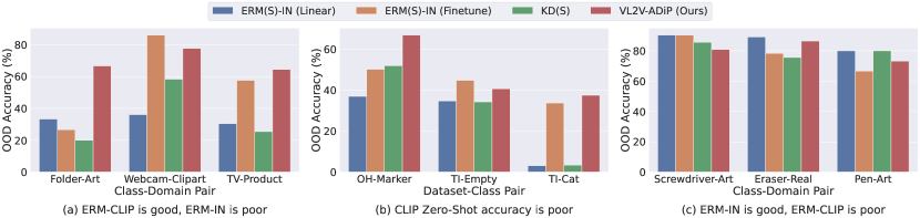
Figure 2: OOD accuracy (%) of the proposed approach when compared to KD and ERM baselines for select classes/ domains in OfficeHome and Terra-Incognita datasets, where the (a) ERM-IN (linear)/ (b) CLIP Zero-shot/ (c) ERM-CLIP (linear) performance is poor.

Table 5: Ablation Study of the proposed VL2V-ADiP: Performance (%) on ViT-B/16 model with ImageNet initialization.

Method - Changes done w.r.t. VL2V-ADiP (Ours)	OH	TI	VLCS	PACS	Avg-ID	Avg-OOD
VL2V-ADiP (Ours)	85.74	55.43	81.90	94.94	92.74	79.50
A1: Combining ”Align” and ”Distill” stages	74.55	52.99	80.14	85.29	90.55	73.24
A2: Without freezing projection head in Stage-2	86.13	56.68	81.78	93.75	93.00	79.59
A3: Distilling only from Text encoder in Stages-1 and 2	83.18	47.02	79.83	90.86	91.87	75.22
A4: Distilling only from Image encoder in Stages-1 and 2	78.97	28.97	82.24	89.97	74.09	70.04
A5: Finetuning CLIP classifier-head in Stage-3 (CE loss) - CLIP init classifier	84.47	49.28	81.30	93.54	93.06	77.15
A6: Finetuning full network in Stage-3 (CE loss) - CLIP init classifier	83.88	49.83	80.13	92.25	93.37	76.52
A7: Finetuning classifier-head in Stage-3 (CE loss) - random init classifier	84.63	49.55	81.29	93.57	93.02	77.26
A8: Finetuning full network in Stage-3 (CE loss) - random init classifier	83.16	50.03	79.78	92.15	93.14	76.28

6.3 Comparison with the SOTA

We present the ID and OOD results of the proposed approach VL2V-ADiP when compared to the DG and KD baselines in Table-3. Gulrajani and Lopez-Paz (2021) show that ERM training is a very strong baseline in DG and outperforms several older methods that were proposed. Thus, ERM training of only the linear layer and ERM fine-tuning of the full network are two important baselines we consider. Further, we present the results of important SOTA methods - SWAD (Cha et al. 2021), MIRO (Cha et al. 2022), DART (Jain et al. 2023), and SAGM (Wang et al. 2023). While there are several methods that outperform ERM (Nam et al. 2021; Kim et al. 2021; Sun and Saenko 2016; Bui et al. 2021), we do not present all of them here since the above-listed recent methods outperform them. We do not compare with the ensembling methods (Arpit et al. 2022; Rame et al. 2023, 2022) since these methods incur additional computational costs of training several diverse models. Since SWAD is a generic method that improves the generalization of any base method by averaging weights across the training iterations, and since we incorporate SWAD in the proposed approach as well, we present all the baseline results by integrating SWAD with each of them and denote them with a suffix “(S)” in the tables. Additionally, we also present two distillation results - (a) knowledge distillation from the VLM teacher to the vision student model as discussed in Section-5.1 and (b) distillation from the VLM teacher using SimKD (Chen et al. 2022). Since the feature distillation methods listed in Sec. 2 cannot be extended to the black box distillation setting, we do not compare with them. The proposed approach VL2V-ADiP achieves $\sim 3.3\%$ improvement on average OOD accuracy across all datasets with respect to the best baselines, with comparable ID accuracy.

6.4 Distillation to lower capacity student models

We present results of distilling from a CLIP ViT-B/16 teacher to different student architectures and capacities (ViT-S/16, DeiT-S, ResNet-50) in Table-4. We observe substantial gains over the Knowledge Distillation and ERM (S) or SWAD baseline across all student architectures. We note that the distillation performance is best when the architecture (ViT) of the teacher matches that of the student. For example, although ViT-S/16, DeiT-S/16, and ResNet-50 have a similar number of parameters, the performance of the ViT-S/16 student is the best, showing the architecture plays a role in the nature of representations learned, thereby allowing better transfer when they match.

6.5 Ablation Study

We present an ablation study of the proposed method in Table-5. Firstly, we study the impact of combining stages-1 (Align) and 2 (Distill), i.e., training the linear projection layer and the backbone jointly in $\mathrm{A}1$. This results in a 2.2% drop in ID accuracy and a 6.3% drop in OOD accuracy, highlighting that the pre-trained ImageNet features are retained better when they are aligned before distillation. In $\mathrm{A}2$, the linear projection head is also trained in Stage-2. The results of this case are similar to the proposed approach, showing that even when the linear head is changed, it does not get updated much after Stage-1 (Align). We next analyze the importance of distilling from both image and text encoders of CLIP by using only one of them individually in $\mathrm{A}3$ and $\mathrm{A}4$. In both cases, we note a significant drop in the OOD accuracy highlighting the importance of distilling from both encoders. Distilling only from the Image encoder has a larger drop due to the lack of alignment between the representations and the classifier head which is composed of CLIP text embeddings corresponding to each of the classes.

In Stage-3 (Predict) of the proposed approach, the CLIP text embeddings corresponding to the classes are directly used as the classifier weights. We explore the impact of training this classifier further using cross-entropy loss over the softmax representations shown in Eq.2, in experiments $\mathrm{A}5$-$\mathrm{A}8$. In $\mathrm{A}5$ and $\mathrm{A}6$, the classifier head is first initialized using the text embeddings of CLIP, and in $\mathrm{A}7$ and $\mathrm{A}8$, a random initialization is used for the classification head. In $\mathrm{A}5$ and $\mathrm{A}7$, only the classifier head is trained, whereas in $\mathrm{A}6$ and $\mathrm{A}8$, the full network is trained. All these experiments result in a drop in the OOD accuracy, indicating that training on the downstream dataset using the cross-entropy loss can destroy the domain invariances learned from CLIP. Since the impact of training the full network is higher, the drop is higher in this case when compared to finetuning only the classification head. In all cases, the In-Domain accuracy improves when compared to the proposed approach, with higher gains in the case when the full network is trained, confirming that training without the supervision of the CLIP teacher indeed overfits to the training domains.

We also compare the ERM and KD baselines with the proposed approach in some of the extreme cases in Fig.2, where the CLIP Image encoder is significantly better than the ERM model (a), and vice-versa (c). For this, we select the classes/domains with the highest difference (40-50%) between the ERM-CLIP (Linear) and ERM-ImageNet (IN) (Linear) baselines from the OfficeHome dataset. We also present the case where the CLIP zero-shot accuracy is poor in OfficeHome (22%) and Terra-Incognita datasets (0%) in Fig.2 (b). The KD baseline relies a lot on the ImageNet pre-trained backbone, hence it is poor when ERM-IN is poor, and is close to our approach when ERM-IN is good. The ERM fine-tuning baseline is best when the ImageNet features are much better than CLIP Image encoder’s features, but it is poor in the other case, as expected. Lastly, even when CLIP zero-shot accuracy is poor (close to 0%), the proposed approach achieves reasonable accuracy, since Stages-1 and 2 align the text embeddings better to the feature extractor, making them more suitable as a classifier.

7 Conclusion

In this work, we aim to leverage the superior generalization of large-scale Vision-Language Models towards improving the OOD generalization of Vision models. We consider a practical scenario where a client gets only black-box access to the model on a pay-per-query basis from the vendor, motivating the need for distilling the model first, and further using the student model during inference. Towards this, we first highlight the unique aspects of the image and text encoders of VLMs and further propose a self-distillation (SD) approach - VL2V-SD, to distill the superior generalization of the VLM’s text encoder to its image encoder, while retaining the rich representations of the latter. We further adapt this to a black-box distillation setting, by firstly projecting the representations of the pre-trained feature-extractor (student) to a space that is aligned with embeddings of the VLM teacher, and further finetuning the backbone using the same. The use of both text and image embeddings induces the rich representations of the VLM and its superior generalization to the student model, while also making the text embeddings more suitable for use in the classification head. Both proposed approaches (VL2V-SD and VL2V-ADiP) achieve substantial gains over prior methods on the popular Domain Generalization datasets. We hope this work would motivate future work toward utilizing the uniqueness and flexibility of multi-modal models for unimodal tasks in an effective manner.

Supplementary Material

The supplementary material presents further details on the proposed approach, datasets, and results. To ensure the reproducibility of our results, we have released our code at https://github.com/val-iisc/VL2V-ADiP.git. The Readme file in the code folder contains details on computational and software requirements as well. The Supplementary is structured as follows:

• Section A: Training Algorithm

• Section B: Details on Datasets

• Section C: Additional Results

  • Section C.1: Variance re-runs

  • Section C.2: Comparison with Additional Baselines

  • Section C.3: Distillation using diverse VLMs

  • Section C.4: Domain-wise Results

• Section D: Analysis on Loss Weighting

Table 6: Domain Generalization Datasets: Details of the five DG datasets recommended on the DomainBed benchmark (Gulrajani and Lopez-Paz 2021)

Dataset	No. of classes	No. of domains	No. of images	Domains	Nature of domain shift
Office-Home (OH)	65	4	15,588	Art, Clipart, Product, Real	Style
Terra-Incognita (TI)	10	4	24,788	L100, L38, L43, L46	Camera location
VLCS	5	4	10,729	Caltech101, LabelMe, SUN09, VOC2007	Photography
PACS	7	4	9,991	Art, Cartoons, Photos, Sketches	Style
DomainNet (DN)	345	6	586,575	Clipart, Infograph, Painting, Quickdraw, Real, Sketch	Style

Appendix A Training Algorithm

The detailed training algorithm of the proposed approach VL2V-ADiP is presented in Algorithm-1. We additionally incorporate SWAD (Cha et al. 2021) during training, which detects the onset of the optimal basin and performs weight-averaging across several model snapshots in the basin. To enable a fair comparison, we present results across all baselines as well using SWAD, denoted using “(S)” in Tables- 2, 3, and 4 of the main paper.

Table 7: Variance across re-runs: Mean and standard deviation of the OOD accuracy (%) of our proposed approach VL2V-ADiP when compared to the ERM (S) and KD (S) baselines across the five Domain Generalization datasets.

Method	Office-Home	Terra-Incognita	VLCS	PACS	DomainNet	Avg-OOD
ERM (S)	82.33 $\pm$ 0.87	48.87 $\pm$ 0.74	80.12 $\pm$ 0.30	90.15 $\pm$ 0.51	56.09 $\pm$ 0.09	71.51 $\pm$ 0.50
KD (S)	81.90 $\pm$ 0.78	48.90 $\pm$ 1.32	79.95 $\pm$ 0.49	90.70 $\pm$ 0.67	56.01 $\pm$ 0.10	71.49 $\pm$ 0.67
VL2V-ADiP (Ours)	85.82 $\pm$ 0.27	55.32 $\pm$ 0.74	82.31 $\pm$ 0.37	94.32 $\pm$ 0.56	59.29 $\pm$ 0.11	75.41 $\pm$ 0.41

Appendix B Details on Datasets

We evaluate the proposed approaches VL2V-SD and VL2V-ADiP on five Domain Generalization datasets that are widely used in literature and recommended on the DomainBed benchmark (Gulrajani and Lopez-Paz 2021). The details of these five datasets are presented in Table-6. This includes diverse datasets with several unique aspects such as - less training data (Fang, Xu, and Rockmore 2013; Li et al. 2017; Venkateswara et al. 2017) and a larger amount of training data (Peng et al. 2019), small domain-shifts (Fang, Xu, and Rockmore 2013) and larger domain shifts (Peng et al. 2019), lesser number of classes (Fang, Xu, and Rockmore 2013; Li et al. 2017) and a higher number of classes (Peng et al. 2019; Venkateswara et al. 2017). We compare against several baselines on each of these individual datasets and also report the average performance across all datasets as is the standard practice (Gulrajani and Lopez-Paz 2021).

Algorithm 1 VL2V - Align, Distill, Predict (ADiP)

1:Input: Let $\mathcal{D}_{s}=\{D_{i},\;\forall i=1,2,\dots d-1\}$ be the data from $d-1$ source domains, $(x_{i},y_{i})\sim{D}_{s}$ be an image-label pair from source domains, $x_{i}^{\mathrm{target}}$ be a test image from the target domain, $f_{T}^{{text}}$ and $f_{T}^{{img}}$ be the text and image encoders of the VLM Teacher respectively, $f_{S}^{{fe}}$ and $f_{S}^{{proj}}$ be the feature extractor and linear projection layer of the student vision model respectively, $h_{\mathrm{VLM}}$ be the zero-shot classifier of the VLM teacher, and $C$ be the set of all class names in dataset $\mathcal{D}_{s}$. For the data sample $(x_{i},y_{i})$, let $\mathbf{I}_{x_{i}}^{t}$ and $\mathbf{T}_{y_{i}}$ be the image and text embeddings from the VLM teacher respectively, and $\textbf{PF}_{x_{i}}^{s}$ be the projected features from the student.

2:$P_{c}=\textrm{``A photo of a $c$''}$ $~{}\forall~{}c\in C$

3:$\mathbf{T}_{c}=f_{T}^{text}(P_{c})$ $~{}\forall~{}c\in C$

4:Stage 1 - Align$\triangleright$ Projection layer trained

5:for $\textrm{\emph{iter}}<\textrm{\emph{MaxIters}}$ do:

6:     Sample batch $(x_{i},y_{i})$ from $\mathcal{D}_{s}$, $\forall~{}~{}0\leq i<n$

7:     $\textbf{I}^{t}_{x_{i}}\leftarrow f_{T}^{{img}}(x_{i})$, $\forall~{}~{}0\leq i<n$

8:     $\mathbf{PF}^{s}_{x_{i}}\leftarrow f_{S}^{proj}(f_{S}^{fe}(x_{i}))$, $\forall~{}~{}0\leq i<n$

9:     $\mathcal{L}=-\frac{1}{2n}\sum_{i}\big{\{}\cos(\textbf{PF}^{s}_{x_{i}},\textbf{T}_{y_{i}})+\cos(\textbf{PF}^{s}_{x_{i}},\textbf{I}^{t}_{x_{i}})\big{\}}$

10:     $\theta_{proj}\leftarrow\theta_{proj}-\nabla_{\theta_{proj}}\mathcal{L}$

11:end for

12:Stage 2 - Distill$\triangleright$ Feature extractor trained

13:for $\textrm{\emph{iter}}<\textrm{\emph{MaxIters}}$ do:

14:     Sample batch $(x_{i},y_{i})$ from $\mathcal{D}_{s}$, $\forall~{}~{}0\leq i<n$

15:     $\mathbf{I}^{t}_{x_{i}}\leftarrow f_{T}^{img}(x_{i}),\forall~{}~{}0\leq i<n$

16:     $\mathbf{PF}^{S}_{x_{i}}\leftarrow f_{S}^{proj}(f_{S}^{fe}(x_{i})),\forall~{}~{}0\leq i<n$

17:     $\mathcal{L}=-\frac{1}{2n}\sum_{i}\big{\{}\cos(\textbf{PF}^{s}_{x_{i}},\textbf{T}_{y_{i}})+\cos(\textbf{PF}^{s}_{x_{i}},\textbf{I}^{t}_{x_{i}})\big{\}}$

18:     $\theta_{fe}\leftarrow\theta_{fe}-\nabla_{\theta_{fe}}\mathcal{L}$

19:end for

20:Stage 3 - Predict

21:$h_{\mathrm{VLM}}(\textbf{x}):=[~{}\cos(\textbf{x},\mathbf{T}_{c}),~{}\forall~{}c\in C~{}]$

22:$\textbf{PF}^{s}_{x_{i}^{\mathrm{target}}}\leftarrow f_{S}^{proj}(f_{S}^{fe}(x_{i}^{\mathrm{target}}))$

23:$\hat{y}_{i}=\mathrm{argmax}_{c}~{}h_{\mathrm{VLM}}(\mathbf{PF}^{s}_{x_{i}^{\mathrm{target}}})$

Appendix C Additional Results

C.1 Variance re-runs

The results in Tables-2, 3, 4, and 5 of the main paper are reported with a fixed seed of 0 using the code shared along with the Supplementary submission, in order to ensure reproducibility of results. In Table-7, we report the mean and standard deviation of the proposed method VL2V-ADiP across 3 re-runs with different random seeds, and compare with the best baselines - ERM Fine-tuned (S) and KD (S) (Hinton, Vinyals, and Dean 2015) where “(S)” denotes that SWAD (Cha et al. 2021) has been used along with the base algorithm. We note that the proposed method shows consistent gains over both baselines, with the standard deviation comparable to the baselines on the respective datasets.

Figure 3: OOD and ID accuracy (%) of the proposed approach VL2V-ADiP across variation in loss weight $\lambda$ for 4 Domain Generalization datasets. Cosine similarity of the student’s projected features w.r.t. the text embeddings of the VLM teacher is given a weight of $(1-\lambda)$, while that w.r.t. the image embeddings of the VLM is given a weight of $\lambda$.

Table 8: SOTA comparison with CLIP initialization (extended comparisons): Performance (%) of the proposed self-distillation approach VLV2-SD, compared to the SOTA DG methods. ViT-B/16 architecture is used with CLIP initialization.

Method	OH	TI	VLCS	PACS	DN	Avg-OOD
CLIP Zero-Shot	82.40	34.10	82.30	96.50	57.70	70.60
ERM Finetuning	68.00	36.52	78.30	81.79	48.71	62.66
MIRO	82.50	54.30	82.20	95.60	54.00	73.72
DART	77.35	46.41	77.04	91.45	56.53	69.76
SAGM	81.11	54.29	81.11	90.61	53.59	72.14
ERM (S) Finetuning	81.01	42.92	79.13	91.35	57.92	70.47
MIRO (S)	84.80	59.30	82.30	96.44	60.47	76.66
DART (S)	80.93	51.24	80.38	93.43	59.32	73.06
SAGM (S)	83.40	58.64	82.05	94.31	59.05	75.49
VL2V - SD (Ours)	87.38	58.54	83.25	96.68	62.79	77.73

Table 9: SOTA comparison with ImageNet-1K initialization (extended comparisons): Performance (%) of the proposed approach VLV2-ADiP, compared to the SOTA DG methods. ViT-B/16 architecture is used with ImageNet-1K initialization.

Method	OH	TI	VLCS	PACS	DN	Avg-OOD
ERM Fine-tuning	78.03	42.53	78.13	85.32	50.84	66.97
KD	77.62	38.66	79.73	84.87	50.73	66.32
MIRO	74.88	44.52	80.39	81.53	49.95	66.25
DART	82.56	50.70	79.70	89.76	56.13	71.77
SAGM	80.87	52.38	79.53	87.29	54.04	70.82
ERM Fine-tuning (S)	83.22	50.05	80.33	90.28	56.10	72.00
KD (S)	82.73	48.40	80.48	91.46	56.11	71.84
MIRO (S)	80.09	50.29	81.10	89.50	55.75	71.35
DART (S)	83.75	49.68	77.29	90.55	58.05	71.86
SAGM (S)	82.22	53.24	79.60	90.02	55.66	72.15
VL2V-ADiP (Ours)	85.74	55.43	81.90	94.13	59.38	75.48

Table 10: Distillation to lower capacity student models: Performance (%) of the proposed approach VL2V-ADiP (denoted as Ours) when compared to existing SOTA DG methods (rows), with different architectures of the student model (columns) on OfficeHome dataset. The teacher architecture is ViT-B/16. (S) denotes SWAD.

Method	ViT-B/16	ViT-S/16	DeiT-S/16	ResNet-50	Avg.
ERM (S)	83.22	78.58	74.95	70.85	76.90
KD (S)	82.73	78.14	74.65	70.67	76.55
SimKD (S)	66.76	54.18	58.75	60.88	60.14
MIRO (S)	80.09	69.45	73.18	72.40	73.78
DART (S)	83.75	79.67	75.85	71.90	77.79
SAGM (S)	82.22	77.00	73.94	70.10	75.81
Ours	85.74	81.22	77.63	74.42	79.75

C.2 Comparison with Additional Baselines

We present additional baseline results corresponding to Tables-2, 3 and 4 of the main paper in Tables-8, 9 and 10 respectively for the sake of completeness. In Tables-8 and 9, we additionally present the respective baseline results without including SWAD (Cha et al. 2021) during training. In Table-10, we compare the performance of the proposed approach VL2V-ADiP on the OfficeHome dataset, with all the baselines considered in Table-3 of the main paper, on student models with different architectures. The proposed approaches show gains across baselines in all the tables.

C.3 Distillation using diverse VLMs

We demonstrate the compatibility of the proposed method VL2V-ADiP with VLMs other than CLIP in Table-11. Specifically, we show results by distilling from FLAVA (Singh et al. 2022), BLIP (Li et al. 2022a), and the data-efficient versions (Li et al. 2022b) of CLIP and FILIP (Yao et al. 2022). We observe that our method achieves the highest gains over the KD baseline (Hinton, Vinyals, and Dean 2015) with CLIP, where the teacher VLM has been trained with a large pre-training dataset. However, our method achieves significant gains even with VLMs pre-trained on smaller datasets.

Table 11: Distillation using various VLMs: Performance (%) of the proposed approach VL2V-ADiP (denoted as Ours) on 4 DG datasets, when distilling from FLAVA (Singh et al. 2022), BLIP (Li et al. 2022a), CLIP (Radford et al. 2021) and the data-efficient versions (Li et al. 2022b) of CLIP and FILIP (Yao et al. 2022). Both the teacher and student architectures are ViT-B/16 in all cases.

Teacher	Method	OH	VLCS	PACS	TI	Avg.	Dataset
FLAVA ViT-B/16	Zero-shot	69.99	79.21	91.34	28.85	67.35	PMD Corpus 70M
	KD (S)	82.50	80.41	90.71	50.86	76.12
	Ours	84.16	82.94	93.22	54.56	78.72
BLIP ViT-B/16	Zero-shot	84.83	71.60	92.23	29.75	69.60	CapFilt (PS) 129M
	KD (S)	82.45	80.31	87.73	48.03	74.63
	Ours	85.86	81.60	94.10	52.07	78.41
CLIP ViT-B/16	Zero-shot	81.57	82.55	95.99	31.15	72.81	CLIP-400M
	KD (S)	82.73	80.48	91.49	48.33	75.76
	Ours	85.74	81.89	94.13	55.43	79.30
DeCLIP ViT-B/32	Zero-shot	43.46	77.79	83.69	27.70	58.16	YFCC-15M
	KD (S)	81.84	79.95	89.96	49.49	75.31
	Ours	82.85	81.40	92.16	50.50	76.73
DeFILIP ViT-B/32	Zero-shot	46.97	74.08	82.02	16.34	54.85	YFCC-15M
	KD (S)	82.14	79.53	90.68	50.96	75.83
	Ours	83.11	81.43	92.03	51.69	77.06

C.4 Domain-wise Results

Table 12: Domain-wise performance (%) of the proposed approaches VL2V-SD and VL2V-ADiP when compared to the respective baselines, on individual domains of all Domain Generalization datasets on the DomainBed benchmark (Gulrajani and Lopez-Paz 2021).

(a) Domain-wise OOD accuracy on Office-Home

Method	Initialization	Art	Clipart	Product	Real	Avg.
CLIP Zero-Shot	CLIP ViT-B / 16	82.56	68.15	89.40	89.50	82.40
ERM (S) Fine-tune		80.12	70.25	86.18	87.49	81.01
MIRO (S)		83.57	75.72	89.70	90.22	84.80
DART (S)		78.79	72.71	86.04	86.17	80.93
SAGM (S)		82.60	72.94	88.94	89.13	83.40
VL2V-SD (Ours)		87.33	78.55	91.98	91.65	87.38
ERM (S) Fine-tune	ImageNet-1k ViT-B / 16	82.24	72.19	88.43	90.02	83.22
KD (S)		80.79	70.76	89.08	90.30	82.73
MIRO (S)		78.89	64.15	87.70	89.62	80.09
DART (S)		81.72	73.17	89.64	90.48	83.75
SAGM (S)		80.23	70.16	88.46	90.02	82.22
VL2V-ADiP (Ours)		84.81	75.92	90.65	91.60	85.74

(b) Domain-wise OOD accuracy on Terra-Incognita

Method	Initialization	L100	L38	L43	L46	Avg.
CLIP Zero-Shot	CLIP ViT-B/16	51.65	20.03	33.60	31.49	34.19
ERM (S) Fine-tune		38.94	38.03	54.03	40.68	42.92
MIRO (S)		67.15	50.75	66.63	52.71	59.31
DART (S)		56.82	37.34	62.31	42.26	49.68
SAGM (S)		72.21	50.10	62.50	49.73	58.64
VL2V-SD (Ours)		69.10	48.40	63.10	53.56	58.54
ERM (S) Fine-tune	ImageNet-1k ViT-B/16	58.98	37.76	58.31	45.15	50.05
KD (S)		61.09	33.21	57.84	41.17	48.33
MIRO (S)		61.27	38.14	57.68	44.08	50.30
DART (S)		56.82	37.34	62.31	42.26	49.68
SAGM (S)		64.17	44.42	59.64	44.74	53.24
VL2V-ADiP (Ours)		62.93	44.83	60.71	53.26	55.43

(c) Domain-wise OOD accuracy on VLCS

Method	Initialization	Caltech	LabelMe	VOC07	SUN09	Avg.
CLIP Zero-Shot	CLIP ViT-B / 16	100.00	69.02	84.19	74.86	82.02
ERM (S) Fine-tune		99.12	63.31	79.01	75.08	79.13
MIRO (S)		97.53	66.59	81.57	83.53	82.30
DART (S)		99.12	65.73	81.07	75.63	80.38
SAGM (S)		97.73	65.86	83.77	80.85	82.05
VL2V-SD (Ours)		99.24	67.81	86.89	79.05	83.25
ERM (S) Fine-tune	ImageNet-1k ViT-B / 16	98.49	64.05	82.60	76.17	80.33
KD (S)		98.87	65.32	81.33	76.39	80.48
MIRO (S)		99.75	64.79	82.66	77.20	81.10
DART (S)		94.08	63.11	76.12	75.86	77.29
SAGM (S)		98.49	64.92	79.32	75.68	79.60
VL2V-ADiP (Ours)		99.62	66.60	82.87	78.46	81.89

(d) Domain-wise OOD accuracy on PACS

Method	Initialization	Art	Cartoon	Photo	Sketch	Avg.
CLIP Zero-Shot	CLIP ViT-B / 16	97.44	99.31	99.93	89.44	96.53
ERM (S) Fine-tune		91.34	89.07	97.53	87.47	91.35
MIRO (S)		98.05	97.50	99.78	90.46	96.44
DART (S)		94.45	92.27	98.80	88.20	93.43
SAGM (S)		95.18	93.60	99.03	89.41	94.30
VL2V-SD (Ours)		98.05	98.19	99.93	90.55	96.68
ERM (S) Fine-tune	ImageNet-1k ViT-B / 16	93.78	86.25	99.18	81.93	90.28
KD (S)		94.20	86.35	99.25	86.04	91.46
MIRO (S)		94.69	85.98	99.63	77.70	89.50
DART (S)		94.45	86.67	99.55	81.52	90.55
SAGM (S)		93.72	86.57	99.18	80.63	90.02
VL2V-ADiP (Ours)		95.61	92.38	99.85	88.68	94.13

(e) Domain-wise OOD accuracy on DomainNet

Method	Initialization	Clipart	Infograph	Painting	Quickdraw	Real	Sketch	Avg.
CLIP Zero-Shot	CLIP ViT-B / 16	72.61	47.08	66.02	14.13	83.12	63.18	57.69
ERM (S) Fine-tune		77.10	38.32	66.13	25.02	75.19	65.76	57.92
MIRO (S)		79.70	43.50	67.36	24.62	79.22	68.42	60.47
DART (S)		78.51	39.99	66.89	25.85	76.37	68.29	59.32
SAGM (S)		78.78	40.21	67.31	24.18	76.29	67.54	59.05
VL2V-SD (Ours)		79.96	49.00	71.05	23.34	82.05	71.36	62.79
ERM (S) Fine-tune	ImageNet-1k ViT-B / 16	76.34	30.92	64.76	21.30	77.70	65.60	56.10
KD (S)		76.56	31.29	64.55	21.44	77.62	65.23	56.11
MIRO (S)		76.32	30.96	64.52	20.18	77.88	64.63	55.75
DART (S)		77.62	34.14	67.64	21.05	80.73	67.11	58.05
SAGM (S)		76.67	29.85	64.42	20.68	77.58	64.58	55.63
VL2V-ADiP (Ours)		78.80	36.86	69.21	21.32	81.33	68.79	59.38

We present results of the proposed approaches VL2V-SD and VL2V-ADiP on each of the individual domains in Tables-12(a) (Office-Home), 12(b) (Terra-Incognita), 12(c) (VLCS), 12(d) (PACS) and 12(e) (DomainNet). The domain in the column heading indicates the unseen test domain, where the training was done on the remaining $d-1$ domains mentioned in Table-6. We note that the proposed methods VL2V-SD and VL2V-ADiP outperform existing methods across several datasets and domains.

VL2V-ADiP achieves the highest gains in cases where domain shift is maximal, highlighting the benefit of using the supervision from CLIP in improving OOD generalization on downstream tasks. The domains with the highest gains include ClipArt (OH), Location-38 (TI), Location-46 (TI), Cartoon (PACS), Infograph (DN), and Painting (OH). The domains with the least gains include Product (OH), Real-World (OH), Art (PACS), Photo (PACS), Quickdraw (DN), and all domains in VLCS. It is intuitive to see that most of the domains with the least gains are the cases where the target distribution is similar to at least one of the source distributions, making them less challenging to evaluate OOD robustness. For example, there is no real domain shift in VLCS, apart from the fact that each split is obtained from a different dataset, with a possible domain shift due to photography differences, which can be considered minor. Hence, taking the supervision of a CLIP model is the least beneficial here.

Appendix D Analysis on Loss Weighting

The training loss of the proposed approach VL2V-ADiP presented in Eq.5 of the main paper, and in L8 and L15 of Algorithm-1, considers equal weights on both loss terms - cosine similarity of the image embeddings $\mathbf{PF}^{s}_{x_{i}}$ w.r.t. text and image embeddings of the VLM teacher respectively. In this section, we explore the impact of varying these weights as a convex interpolation between the cosine similarity w.r.t. text embeddings (weighted by $1-\lambda$) and image embeddings (weighted by $\lambda$) respectively as shown below:

$$\mathcal{L}=-\frac{1}{2n}\sum_{i=1}^{n}\big{\{}(1-\lambda)\cdot\cos(\textbf{PF}^{s}_{x_{i}},\textbf{T}_{y_{i}})+\lambda\cdot\cos(\textbf{PF}^{s}_{x_{i}},\textbf{I}^{t}_{x_{i}})\big{\}}$$ (6)

We note from the plots in Fig.3 that while the best OOD accuracy could be achieved at a different $\lambda$ value, a setting of 0.5 works reasonably well, since the proposed approach is not too sensitive to variations in $\lambda$ in most cases. Moreover, a value of 0.5 assigns equal weightage to losses w.r.t. both image and text embeddings (since they are of the same scale), which is the best setting to consider in the absence of hyperparameter tuning.

References

- Arjovsky et al. (2019) Arjovsky, M.; Bottou, L.; Gulrajani, I.; and Lopez-Paz, D. 2019. Invariant risk minimization. arXiv preprint arXiv:1907.02893.
- Arpit et al. (2022) Arpit, D.; Wang, H.; Zhou, Y.; and Xiong, C. 2022. Ensemble of averages: Improving model selection and boosting performance in domain generalization. Advances in Neural Information Processing Systems (NeurIPS), 35.
- Beery, Van Horn, and Perona (2018) Beery, S.; Van Horn, G.; and Perona, P. 2018. Recognition in terra incognita. In European conference on computer vision (ECCV). Springer.
- Biggio, Nelson, and Laskov (2012) Biggio, B.; Nelson, B.; and Laskov, P. 2012. Poisoning Attacks against Support Vector Machines. In International Conference on Machine Learning (ICML). PMLR.
- Blanchard et al. (2021) Blanchard, G.; Deshmukh, A. A.; Dogan, Ü.; Lee, G.; and Scott, C. 2021. Domain generalization by marginal transfer learning. The Journal of Machine Learning Research (JMLR), 22(1).
- Bui et al. (2021) Bui, M.-H.; Tran, T.; Tran, A.; and Phung, D. 2021. Exploiting domain-specific features to enhance domain generalization. Advances in Neural Information Processing Systems (NeurIPS), 34.
- Carlini et al. (2023) Carlini, N.; Jagielski, M.; Choquette-Choo, C. A.; Paleka, D.; Pearce, W.; Anderson, H.; Terzis, A.; Thomas, K.; and Tramèr, F. 2023. Poisoning Web-Scale Training Datasets is Practical. arXiv preprint arXiv:2302.10149.
- Cha et al. (2021) Cha, J.; Chun, S.; Lee, K.; Cho, H.-C.; Park, S.; Lee, Y.; and Park, S. 2021. Swad: Domain generalization by seeking flat minima. Advances in Neural Information Processing Systems (NeurIPS), 34.
- Cha et al. (2022) Cha, J.; Lee, K.; Park, S.; and Chun, S. 2022. Domain Generalization by Mutual-Information Regularization with Pre-trained Models. European conference on computer vision (ECCV).
- Changpinyo et al. (2021) Changpinyo, S.; Sharma, P.; Ding, N.; and Soricut, R. 2021. Conceptual 12M: Pushing Web-Scale Image-Text Pre-Training To Recognize Long-Tail Visual Concepts. In Proceedings of the IEEE/CVF Conference on Computer Vision and Pattern Recognition (CVPR).
- Chattopadhyay, Balaji, and Hoffman (2020) Chattopadhyay, P.; Balaji, Y.; and Hoffman, J. 2020. Learning to balance specificity and invariance for in and out of domain generalization. In European conference on computer vision (ECCV). Springer.
- Chen et al. (2022) Chen, D.; Mei, J.-P.; Zhang, H.; Wang, C.; Feng, Y.; and Chen, C. 2022. Knowledge distillation with the reused teacher classifier. In Proceedings of the IEEE/CVF conference on computer vision and pattern recognition (CVPR).
- Chen et al. (2021a) Chen, D.; Mei, J.-P.; Zhang, Y.; Wang, C.; Wang, Z.; Feng, Y.; and Chen, C. 2021a. Cross-layer distillation with semantic calibration. In Proceedings of the AAAI Conference on Artificial Intelligence (AAAI).
- Chen et al. (2021b) Chen, P.; Liu, S.; Zhao, H.; and Jia, J. 2021b. Distilling knowledge via knowledge review. In Proceedings of the IEEE/CVF Conference on Computer Vision and Pattern Recognition (CVPR).
- Dosovitskiy et al. (2021) Dosovitskiy, A.; Beyer, L.; Kolesnikov, A.; Weissenborn, D.; Zhai, X.; Unterthiner, T.; Dehghani, M.; Minderer, M.; Heigold, G.; Gelly, S.; et al. 2021. An image is worth 16x16 words: Transformers for image recognition at scale.
- Fang, Xu, and Rockmore (2013) Fang, C.; Xu, Y.; and Rockmore, D. N. 2013. Unbiased Metric Learning: On the Utilization of Multiple Datasets and Web Images for Softening Bias. In Proceedings of the IEEE/CVF International Conference on Computer Vision (ICCV).
- Ganin et al. (2016) Ganin, Y.; Ustinova, E.; Ajakan, H.; Germain, P.; Larochelle, H.; Laviolette, F.; Marchand, M.; and Lempitsky, V. 2016. Domain-Adversarial Training of Neural Networks. The Journal of Machine Learning Research (JMLR), 17(1).
- Gulrajani and Lopez-Paz (2021) Gulrajani, I.; and Lopez-Paz, D. 2021. In Search of Lost Domain Generalization. In International Conference on Learning Representations (ICLR).
- Hinton, Vinyals, and Dean (2015) Hinton, G.; Vinyals, O.; and Dean, J. 2015. Distilling the knowledge in a neural network. arXiv preprint arXiv:1503.02531.
- Huang et al. (2020) Huang, Z.; Wang, H.; Xing, E. P.; and Huang, D. 2020. Self-challenging improves cross-domain generalization. In European conference on computer vision (ECCV). Springer.
- Jain et al. (2023) Jain, S.; Addepalli, S.; Sahu, P. K.; Dey, P.; and Babu, R. V. 2023. DART: Diversify-Aggregate-Repeat Training Improves Generalization of Neural Networks. In Proceedings of the IEEE/CVF Conference on Computer Vision and Pattern Recognition (CVPR).
- Jia et al. (2021) Jia, C.; Yang, Y.; Xia, Y.; Chen, Y.-T.; Parekh, Z.; Pham, H.; Le, Q.; Sung, Y.-H.; Li, Z.; and Duerig, T. 2021. Scaling up visual and vision-language representation learning with noisy text supervision. In International Conference on Machine Learning (ICML). PMLR.
- Kim et al. (2021) Kim, D.; Yoo, Y.; Park, S.; Kim, J.; and Lee, J. 2021. Selfreg: Self-supervised contrastive regularization for domain generalization. In Proceedings of the IEEE/CVF International Conference on Computer Vision (ICCV).
- Kim, Son, and Kim (2021) Kim, W.; Son, B.; and Kim, I. 2021. Vilt: Vision-and-language transformer without convolution or region supervision. In International conference on machine learning (ICML). PMLR.
- Krizhevsky, Sutskever, and Hinton (2012) Krizhevsky, A.; Sutskever, I.; and Hinton, G. E. 2012. Imagenet classification with deep convolutional neural networks. In Advances in Neural Information Processing Systems (NeurIPS).
- Krueger et al. (2021) Krueger, D.; Caballero, E.; Jacobsen, J.-H.; Zhang, A.; Binas, J.; Zhang, D.; Le Priol, R.; and Courville, A. 2021. Out-of-distribution generalization via risk extrapolation (rex). In International conference on machine learning (ICML). PMLR.
- LeCun, Bengio, and Hinton (2015) LeCun, Y.; Bengio, Y.; and Hinton, G. 2015. Deep learning. nature, 521(7553).
- Li et al. (2018a) Li, D.; Yang, Y.; Song, Y.-Z.; and Hospedales, T. 2018a. Learning to Generalize: Meta-learning for Domain Generalization. In Proceedings of the AAAI Conference on Artificial Intelligence (AAAI).
- Li et al. (2017) Li, D.; Yang, Y.; Song, Y.-Z.; and Hospedales, T. M. 2017. Deeper, Broader and Artier Domain Generalization. In Proceedings of the IEEE/CVF International Conference on Computer Vision (ICCV).
- Li et al. (2018b) Li, H.; Pan, S. J.; Wang, S.; and Kot, A. C. 2018b. Domain generalization with adversarial feature learning. In Proceedings of the IEEE/CVF Conference on Computer vision and pattern recognition (CVPR).
- Li et al. (2018c) Li, H.; Pan, S. J.; Wang, S.; and Kot, A. C. 2018c. Domain Generalization with Adversarial Feature Learning. In Proceedings of the IEEE/CVF Conference on Computer vision and pattern recognition (CVPR).
- Li et al. (2022a) Li, J.; Li, D.; Xiong, C.; and Hoi, S. 2022a. Blip: Bootstrapping language-image pre-training for unified vision-language understanding and generation. In International Conference on Machine Learning (ICML). PMLR.
- Li et al. (2018d) Li, Y.; Gong, M.; Tian, X.; Liu, T.; and Tao, D. 2018d. Domain generalization via conditional invariant representations. In Proceedings of the AAAI Conference on Artificial Intelligence (AAAI).
- Li et al. (2022b) Li, Y.; Liang, F.; Zhao, L.; Cui, Y.; Ouyang, W.; Shao, J.; Yu, F.; and Yan, J. 2022b. Supervision Exists Everywhere: A Data Efficient Contrastive Language-Image Pre-training Paradigm. In International Conference on Learning Representations (ICLR).
- Liu et al. (2023) Liu, D.; Kan, M.; Shan, S.; and Chen, X. 2023. Function-consistent feature distillation. In International Conference on Learning Representations (ICLR).
- Lu et al. (2019) Lu, J.; Batra, D.; Parikh, D.; and Lee, S. 2019. Vilbert: Pretraining task-agnostic visiolinguistic representations for vision-and-language tasks. Advances in Neural Information Processing Systems (NeurIPS), 32.
- Lv et al. (2022) Lv, F.; Liang, J.; Li, S.; Zang, B.; Liu, C. H.; Wang, Z.; and Liu, D. 2022. Causality inspired representation learning for domain generalization. In Proceedings of the IEEE/CVF Conference on Computer vision and pattern recognition (CVPR).
- Menon and Vondrick (2023) Menon, S.; and Vondrick, C. 2023. Visual classification via description from large language models. In International Conference on Learning Representations (ICLR).
- Nam et al. (2021) Nam, H.; Lee, H.; Park, J.; Yoon, W.; and Yoo, D. 2021. Reducing domain gap by reducing style bias. In Proceedings of the IEEE/CVF Conference on Computer vision and pattern recognition (CVPR).
- Nuriel, Benaim, and Wolf (2021) Nuriel, O.; Benaim, S.; and Wolf, L. 2021. Permuted adain: Reducing the bias towards global statistics in image classification. In Proceedings of the IEEE/CVF Conference on Computer vision and pattern recognition (CVPR).
- Passban et al. (2021) Passban, P.; Wu, Y.; Rezagholizadeh, M.; and Liu, Q. 2021. Alp-kd: Attention-based layer projection for knowledge distillation. In Proceedings of the AAAI Conference on artificial intelligence (AAAI).
- Peng et al. (2019) Peng, X.; Bai, Q.; Xia, X.; Huang, Z.; Saenko, K.; and Wang, B. 2019. Moment matching for multi-source domain adaptation. In Proceedings of the IEEE/CVF International Conference on Computer Vision (ICCV).
- Piratla, Netrapalli, and Sarawagi (2020) Piratla, V.; Netrapalli, P.; and Sarawagi, S. 2020. Efficient domain generalization via common-specific low-rank decomposition. In International conference on machine learning (ICML). PMLR.
- Radford et al. (2021) Radford, A.; Kim, J. W.; Hallacy, C.; Ramesh, A.; Goh, G.; Agarwal, S.; Sastry, G.; Askell, A.; Mishkin, P.; Clark, J.; et al. 2021. Learning transferable visual models from natural language supervision. In International Conference on Machine Learning (ICML). PMLR.
- Radford et al. (2019) Radford, A.; Wu, J.; Child, R.; Luan, D.; Amodei, D.; Sutskever, I.; et al. 2019. Language models are unsupervised multitask learners. OpenAI blog, 1(8): 9.
- Rame et al. (2023) Rame, A.; Ahuja, K.; Zhang, J.; Cord, M.; Bottou, L.; and Lopez-Paz, D. 2023. Model ratatouille: Recycling diverse models for out-of-distribution generalization.
- Rame et al. (2022) Rame, A.; Kirchmeyer, M.; Rahier, T.; Rakotomamonjy, A.; Gallinari, P.; and Cord, M. 2022. Diverse weight averaging for out-of-distribution generalization. Advances in Neural Information Processing Systems (NeurIPS), 35.
- Robey, Pappas, and Hassani (2021) Robey, A.; Pappas, G. J.; and Hassani, H. 2021. Model-based domain generalization. Advances in Neural Information Processing Systems (NeurIPS), 34.
- Romero et al. (2015) Romero, A.; Ballas, N.; Kahou, S. E.; Chassang, A.; Gatta, C.; and Bengio, Y. 2015. Fitnets: Hints for thin deep nets. In International Conference on Learning Representations (ICLR).
- Sagawa et al. (2019) Sagawa, S.; Koh, P. W.; Hashimoto, T. B.; and Liang, P. 2019. Distributionally robust neural networks for group shifts: On the importance of regularization for worst-case generalization. arXiv preprint arXiv:1911.08731.
- Schuhmann et al. (2021) Schuhmann, C.; Vencu, R.; Beaumont, R.; Kaczmarczyk, R.; Mullis, C.; Katta, A.; Coombes, T.; Jitsev, J.; and Komatsuzaki, A. 2021. Laion-400m: Open dataset of clip-filtered 400 million image-text pairs. arXiv preprint arXiv:2111.02114.
- Shu et al. (2022) Shu, M.; Nie, W.; Huang, D.-A.; Yu, Z.; Goldstein, T.; Anandkumar, A.; and Xiao, C. 2022. Test-Time Prompt Tuning for Zero-Shot Generalization in Vision-Language Models. In Advances in Neural Information Processing Systems (NeurIPS).
- Singh et al. (2022) Singh, A.; Hu, R.; Goswami, V.; Couairon, G.; Galuba, W.; Rohrbach, M.; and Kiela, D. 2022. Flava: A foundational language and vision alignment model. In Proceedings of the IEEE/CVF Conference on Computer Vision and Pattern Recognition (CVPR).
- Su et al. (2020) Su, W.; Zhu, X.; Cao, Y.; Li, B.; Lu, L.; Wei, F.; and Dai, J. 2020. VL-BERT: Pre-training of Generic Visual-Linguistic Representations. In International Conference on Learning Representations (ICLR).
- Sun and Saenko (2016) Sun, B.; and Saenko, K. 2016. Deep coral: Correlation alignment for deep domain adaptation. In European conference on computer vision (ECCV). Springer.
- Tan and Bansal (2019) Tan, H.; and Bansal, M. 2019. LXMERT: Learning Cross-Modality Encoder Representations from Transformers. In Proceedings of the Conference on Empirical Methods in Natural Language Processing (EMNLP).
- Thomee et al. (2016) Thomee, B.; Shamma, D. A.; Friedland, G.; Elizalde, B.; Ni, K.; Poland, D.; Borth, D.; and Li, L.-J. 2016. YFCC100M: The new data in multimedia research. Communications of the ACM, 59(2).
- Vaswani et al. (2017) Vaswani, A.; Shazeer, N.; Parmar, N.; Uszkoreit, J.; Jones, L.; Gomez, A. N.; Kaiser, Ł.; and Polosukhin, I. 2017. Attention is all you need. Advances in Neural Information Processing Systems (NeurIPS), 30.
- Venkateswara et al. (2017) Venkateswara, H.; Eusebio, J.; Chakraborty, S.; and Panchanathan, S. 2017. Deep hashing network for unsupervised domain adaptation. In Proceedings of the IEEE/CVF Conference on Computer vision and pattern recognition (CVPR).
- Wang et al. (2023) Wang, P.; Zhang, Z.; Lei, Z.; and Zhang, L. 2023. Sharpness-aware gradient matching for domain generalization. In Proceedings of the IEEE/CVF Conference on Computer Vision and Pattern Recognition (CVPR).
- Wang, Li, and Kot (2020) Wang, Y.; Li, H.; and Kot, A. C. 2020. Heterogeneous domain generalization via domain mixup. In IEEE International Conference on Acoustics, Speech and Signal Processing (ICASSP). IEEE.
- Yao et al. (2022) Yao, L.; Huang, R.; Hou, L.; Lu, G.; Niu, M.; Xu, H.; Liang, X.; Li, Z.; Jiang, X.; and Xu, C. 2022. FILIP: Fine-grained Interactive Language-Image Pre-Training. In International Conference on Learning Representations (ICLR).
- Zhai et al. (2022) Zhai, X.; Wang, X.; Mustafa, B.; Steiner, A.; Keysers, D.; Kolesnikov, A.; and Beyer, L. 2022. Lit: Zero-shot transfer with locked-image text tuning. In Proceedings of the IEEE/CVF Conference on Computer Vision and Pattern Recognition (CVPR).
- Zhang et al. (2021) Zhang, M.; Marklund, H.; Dhawan, N.; Gupta, A.; Levine, S.; and Finn, C. 2021. Adaptive risk minimization: Learning to adapt to domain shift. Advances in Neural Information Processing Systems (NeurIPS), 34.
- Zhou et al. (2022) Zhou, K.; Yang, J.; Loy, C. C.; and Liu, Z. 2022. Learning to prompt for vision-language models. International Journal of Computer Vision (IJCV), 130(9).