Visualizing a Nondeterministic to Deterministic Finite-State Machine Transformation

Abstract.

The transformation of a nondeterministic finite-state automaton into a deterministic finite-state automaton is an integral part of any course on formal languages and automata theory. For some students, understanding this transformation is challenging. Common problems encountered include not comprehending how the states of the deterministic finite-state automaton are determined and not comprehending the role that all the edges of the nondeterministic finite-state automaton have in the deterministic finite-state automaton’s construction. To aid students in understanding, transformation visualization tools have been developed. Although useful in helping students, these tools do not properly illustrate the relationship between the states of the deterministic finite-state automaton and the edges of the nondeterministic finite-state automaton. This article presents a novel interactive visualization tool to illustrate the transformation that highlights this relationship and that is integrated into the FSM programming language. In addition, the implementation of the visualization is sketched.

1. Introduction

Formal Languages and Automata Theory (FLAT) courses and textbooks place a great deal on emphasis on constructive proofs. Constructive proofs are commonly used to establish, for example, the equivalence of different computation models. As part of such proofs, a construction algorithm is designed that transforms one model of computation into another. FLAT students are commonly exposed to the transformation of a nondeterministic finite-state automaton (ndfa) into a deterministic finite-state automaton (dfa). It is important for students to learn about such a transformation, because ndfas are usually easier to design than dfas and dfas are usually easier to implement using a programming language. Therefore, learning about the ndfa to dfa transformation makes it easier to design and write software for string searching (Baase, 1988) and spell checking (Hládek et al., 2020) in word processors, for recognizing tokens, keywords, and identifiers in compilers (Parsons, 1992; Farhanaaz and Sanju, 2016), for specifying communication event sequences in network design (Prithi and Sumathi, 2020), for detecting malicious behavior by cybersecurity software (Ilgun et al., 1995), and for formal software verification (Gheorghe et al., 2010).

More often than desirable, students struggle to understand the ndfa to dfa transformation. This is not entirely surprising, because a path in a dfa transition diagram may represent multiple paths in an ndfa transition diagram. Thus, a state in the dfa under construction may represent any subset of states in the ndfa and an edge in the dfa under construction may represent multiple ndfa edges. We shall call the states in the dfa under construction super states. Mentally or manually tracking super states and path information during the transformation process is taxing and error-prone. To aid students, visualization tools have been developed. These tools build the dfa transition diagram by adding edges in a stepwise manner. Rarely, however, is proper attention given to where super states come from and to the ndfa edges that are represented by a dfa edge. Therefore, there is a need to improve the visualization of this transformation.

This article describes a new visualization tool for the ndfa to dfa transformation developed for FSM–a domain-specific language for the FLAT classroom (Morazán and Antunez, 2014; Morazán et al., 2020). With this new tool, the user may visualize the stepwise addition of dfa-edges while simultaneously visualizing its corresponding ndfa-edges. In addition, the tool also highlights the ndfa edges that are already captured by the dfa under construction. Users may step forward and backward in the dfa construction as well as jump directly to the end of the dfa construction to view the result. The article is structured as follows. Section 2 briefly reviews and contrasts with related work. Section 3 introduces FSM and the constructors for dfas and ndfas. Section 4 describes the implementation of the transformation algorithm in FSM. Section 5 describes the transformation’s visualization. Finally, Section 6 presents concluding remarks and directions for future work.

2. Related Work

2.1. The Transformation

FLAT textbooks usually hinge the conversion from an ndfa, N=(K $\Sigma$ s F $\delta$), to a dfa, D=(K^′ $\Sigma$^′ s^′ F^′ $\delta$^′), on the observation that N may occupy multiple states during a computation (Gurari, 1989; Hopcroft et al., 2006; Lewis and Papadimitriou, 1997; Martin, 2003; Rich, 2019; Sipser, 2013). Namely, the states that N may occupy are the states reachable with the consumed input. To understand which are the reachable states given some input, it is useful to introduce E(q), the notion of the empties of q, where q$\in$K. Informally, the empties of q is the set of states reachable from q using only empty transitions. More formally, the empties of q is defined as follows:

     E(q) = {p | (($\epsilon$ q) $\vdash^{*}$ ($\epsilon$ p))}

D is constructed using the following algorithm:

K^′ = :

2^K, the power set of K

$\Sigma$^′ =:

$\Sigma$

s^′ =:

E(s)

F^′ =:

{B $|$ B$\subseteq$K^′ $\wedge$ B$\cap$F$\neq\emptyset$}

$\delta$^′ =:

{(Q y $\bigcup$E(p)) $|$ p$\in$K $\wedge$ (q y p)$\in$$\delta$ $\wedge$ Q$\in$K${}^{\prime}\wedge$ q$\in$Q}

The states in K^′ are, as mentioned, usually refered to as super states given that each may contain more than one state in K. The algorithm is correct, but it is also terse and, given that the power set of a finite set needs to be computed, not practical for other than small sets of states. Most textbooks, therefore, observe that not all the super states in K^′ are relevant and that the only relevant super states are those that are reachable from E(s). Under this mantle, dfa construction becomes a search for a transition function on super states starting from E(s).

In contrast, the FSM transformation from ndfa to dfa is described and implemented from the start as a search for a transition function on super states. In this manner, students do not need to worry about computing or searching the power set of a set. Instead, they may focus on a breadth-first-based algorithm that searches for the needed super-state transitions. This algorithm requires the computation of a table for the empties of every state in the given ndfa and the computation of an encoding table that maps super states to valid state names in FSM. Such a programming approach appeals to Computer Science students that wish to hone their programming skills. This algorithm is further described in Section 4.

2.2. Visualization

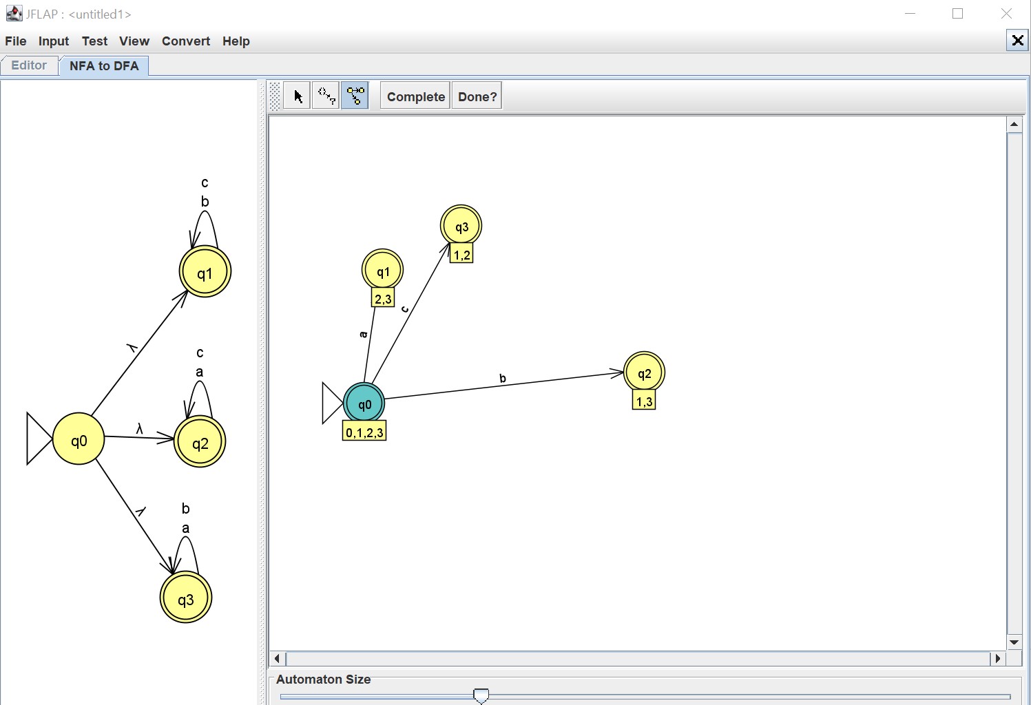
(a) After expanding the starting state.

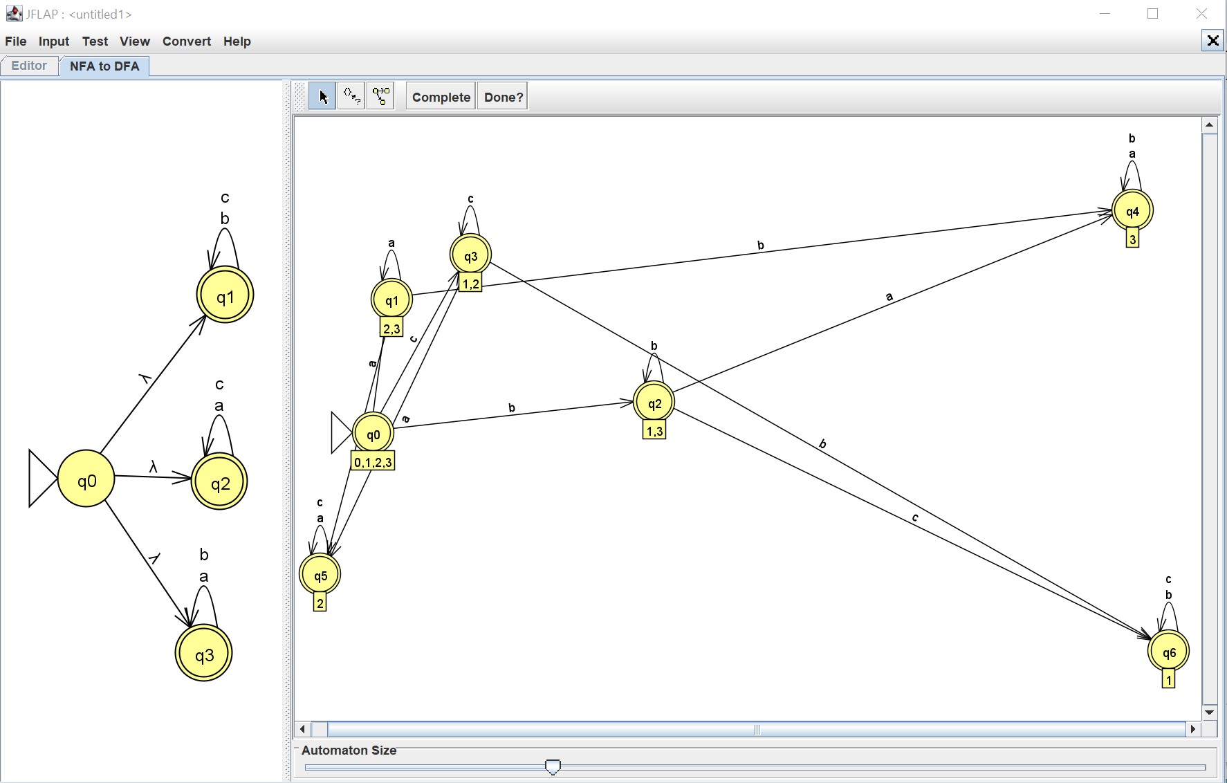
(b) Completed Transformation.

Figure 1. JFLAP visualization.

JFLAP is a visualization tool that allows users to graphically edit ndfas and convert them to dfas (Rodger, 2006; Rodger et al., 2006). The conversion may be done piecemeal on node at a time or may be done in one step. Piecemeal conversion, for example, allows users to click on a super state to generate all the edges out of the clicked super state. Figure 1(a) displays the first such step in such a conversion. The ndfa on the left decides the language (b $\cup$ c)^∗ $\cup$ (a $\cup$ c)^∗ $\cup$ (a $\cup$ b)^∗. The transition diagram for the dfa starts only containing the initial super state. After the initial super state is expanded, three edges are added. Completing the rest of the transformation in one step yields the configuration displayed in Figure 1(b). There are salient features that merit scrutiny. The first is that the dfa transition diagram in Figure 1(b) does not represent a function. It is missing transitions from q4 on an a, from q5 on a b, and from q6 on a c. The missing transitions, clearly, all ought to go to a dead state. This brings us to the second feature that merits scrutiny: there is a missing state. Namely, the dead state. These features can be problematic with a student just starting to study FLAT. After studying the transformation algorithm, they naturally question why every state does not have a transition for every letter in the alphabet. The third feature that merits scrutiny is the layout of the dfa transition diagram. It is unappealing and difficult to read. The fourth issue is that it is not clear, when the graph is constructed piecemeal, which ndfa edges have been used to construct the dfa and which are yet to be used. Finally, the fifth issue is that the piecemeal transformation only runs in one direction. The user is unable to step back to review previous steps.

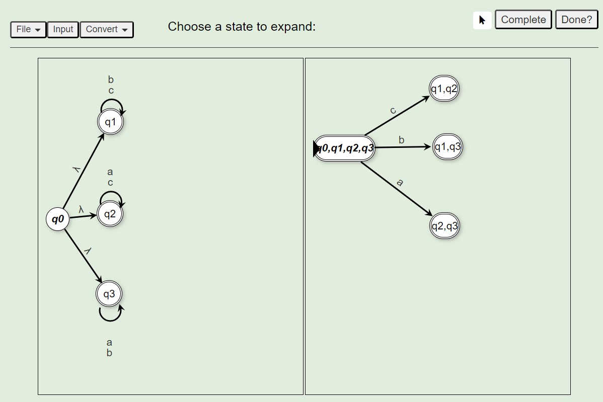
(a) After expanding the starting state.

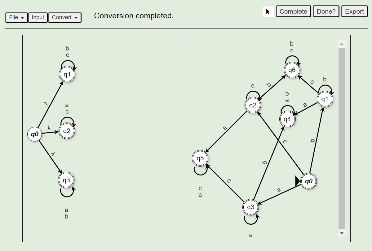
(b) Completed Transformation.

Figure 2. OpenFLAP visualization.

OpenFLAP is another visualization tool that allows users to graphically edit ndfas and convert them to dfas (Mohammed, 2020). This tool demands more interaction with the user when the dfa is built piecemeal. As in JFLAP, the state diagram for the dfa starts with E(s). When a user clicks on a state, she is prompted for the alphabet element to expand on. The user then may place a super state, but first must specify the super state’s member ndfa states. The first three steps of the piecemeal conversion are displayed in Figure 2(a). Observe that the layout is nicer and easier to read than what is produced by JFLAP as displayed in Figure 1(a). The layout is better because the user has chosen to carefully place the super states. Like JFLAP, OpenFLAP allows for the dfa’s completion in one step. The result of such a step is displayed in Figure 2(b). As with JFLAP, the layout is unappealing and difficult to read, the dead state and associated transitions are missing, and, when the dfa is built piecemeal, it is not easy to determine which ndfa edges have been used to construct the dfa and which are yet to be used. Finally, the user is also unable to step back in the piecemeal computation to review previous steps.

In contrast, the work presented in this article completely automates the piecemeal construction of the dfa’s state transition diagram. The user cannot choose the direction of the expansion. Instead, she can step backwards and forwards in the computation. In addition, the user may complete the transformation in one step and still step backwards. Furthermore, GraphViz (Gansner and North, 2000) is used to layout the ndfa and the dfa transition diagrams in an appealing manner. When an edge is added to the dfa, the ndfa edges it accounts for are highlighted in the ndfa’s transition diagram. In this manner, students can easily determine how ndfa and dfa edges correspond. Any ndfa edges previously used in the dfa’s construction are faded, and ndfa edges not yet used in the construction are rendered as solid black edges. Finally, in further contrast with JFLAP and OpenFLAP, the dfa transition graph is complete. That is, it includes a dead state, and associated transitions when needed. The FSM transformation visualization is further discussed in Section 5.

3. Brief Introduction to FSM

3.1. Core Definitions

In FSM, a state is an uppercase Roman alphabet symbol, and an input alphabet symbol is a lowercase Roman alphabet letter or number. An input alphabet, $\Sigma$, is represented as a list of alphabet symbols. A word is either EMP, denoting the empty word, or a nonempty list of alphabet symbols. Each word is given as input to a state machine to decide if it is in the machine’s language.

The machine constructors of interest for this article are those for finite-state automatons:

     make-dfa: K $\Sigma$ s F $\delta$ ['no-dead] $\rightarrow$ dfa
     make-ndfa: K $\Sigma$ s F $\delta$ $\rightarrow$ ndfa

Here, K is a list of states, F is a list of final states in K, s is the starting state in K, and $\delta$ is a transition relation. A transition relation is represented as a list of transition rules. This relation must be a function for a dfa. A dfa transition rule is a triple, (K $\Sigma$ K), containing a source state, the element to read, and a destination state. The optional 'no-dead argument for make-dfa indicates to the constructor that the relation given is a function. Omitting this argument indicates that the transition function is incomplete and the constructor adds a fresh dead state along with transitions to this dead state for any missing transitions. An ndfa transition rule is a triple, (K $\{\Sigma\cup\{EMP\}\}$ K), containing a source state, the element to read (possibly none), and a destination state.

Observers are functions that use a given machine to compute a result. The observers are:

     (sm-states M)  (sm-sigma M) (sm-start M) (sm-finals M)  (sm-rules M)
     (sm-type M)
     (sm-apply M w)
     (sm-showtransitions M w)

The first 5 observers extract a component from the given state machine. The sixth returns the given state machine’s type. The seventh applies the given machine to the given word and returns 'accept or 'reject. The eighth returns a trace of the configurations traversed applying the given machine to the given word ending with the result. A trace is only returned, however, if the machine is a dfa or if the word is accepted by an ndfa.

3.2. Visualization

FSM provides machine rendering and machine execution visualization. The current visualization primitives are:

     (sm-graph M)     (sm-visualize M [(s p)∗])

The (sm-graph M) returns an image of the given machine’s transition diagram. In the returned image, a node represents a state and an edge represents a transition rule. Each node is a state enclosed in a circle variety. The starting state is denoted by a green circle. A final state is denoted by a double black circle. If the starting state is also a final state then it is denoted using a double green circle. All other states are denoted using a single black circle. The label on an edge denotes the element that is consumed using the rule the edge represents.

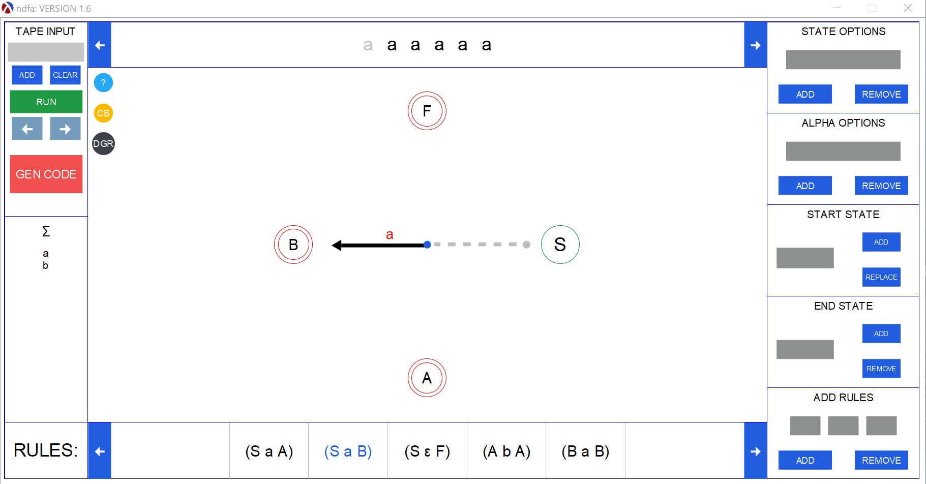
(a) Control view.

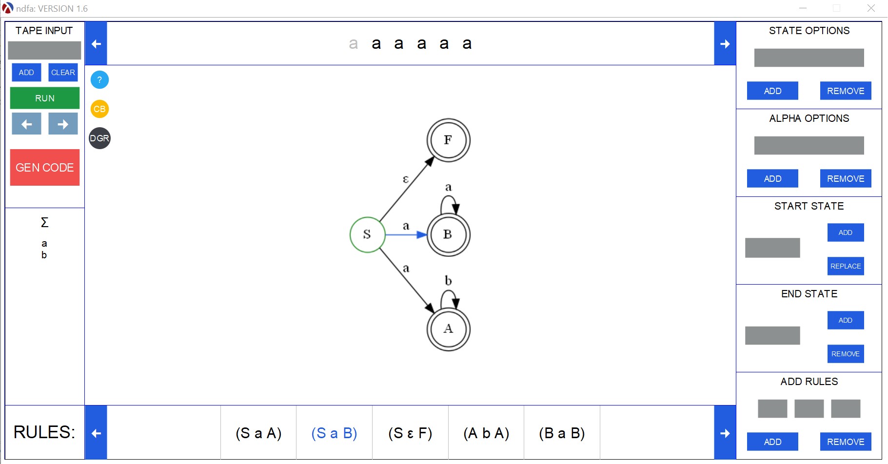
(b) State diagram view.

Figure 3. Execution Visualization for an ndfa Deciding L={$\epsilon\cup aa^{\texttt{*}}\cup ab^{\texttt{*}}$}

The (sm-visualize M [(s p)^∗]) launches the FSM visualization tool to simulate machine execution. The optional two-element lists contain a state of the given machine and an invariant predicate for the state. Machine execution may always be visualized if the machine is a dfa. Similarly to sm-showtransitons, ndfa machine execution may only be visualized if the given word is in the machine’s language. Within the visualization tool, a machine is depicted in control view or in state diagram view. In control view, as depicted in Figure 3(a), final states are denoted using double red circles. The arrow points to the current state and the dashed line indicates the previous state. In Figure 3(a), the last rule used is (S a B). In state diagram view, the machine is depicted as returned by sm-graph. The edge for the last rule used is highlighted in blue. Figure 3(b) depicts the same machine state as in Figure 3(a) in state diagram view. In both views, the right column allows for machine editing, the left column is used to provide an input word and step through machine execution, the top displays the input word, and the bottom displays the transition rules. For further details on machine execution visualization in FSM, the reader is referred to a previous publication (Morazán et al., 2020).

3.3. An Illustrative Example

To illustrate programming in FSM, consider the following example:

     ;; L(LNDFA) = $\epsilon$ $\cup$ aa${}^{\texttt{*}}$ $\cup$ ab${}^{\texttt{*}}$
     (define LNDFA (make-ndfa '(S A B F)
                              '(a b)
                              'S
                              '(A B F)
                              `((S a A)
                                (S a B)
                                (S ,EMP F)
                                (A b A)
                                (B a B))))

     ;; Tests for LNDFA
     (check-equal? (sm-apply LNDFA '(a b a)) 'reject)
     (check-equal? (sm-apply LNDFA '(b b b b b)) 'reject)
     (check-equal? (sm-apply LNDFA '(a b b b b a a a)) 'reject)
     (check-equal? (sm-apply LNDFA '()) 'accept)
     (check-equal? (sm-apply LNDFA '(a)) 'accept)
     (check-equal? (sm-apply LNDFA '(a a a a)) 'accept)
     (check-equal? (sm-apply LNDFA '(a b b)) 'accept)

The language of this machine contains the empty word and all words that start with an a and end with either an arbitrary number of as or an arbitrary number of bs. Essentially, the machine nondeterministically decides if the given word is empty, in ab${}^{\texttt{*}}$, in aa${}^{\texttt{*}}$, or is rejected. The tests validate LNDFA.

Machine traces are:

     > (sm-showtransitions LNDFA '())
     '((() S) (() F) accept)
     > (sm-showtransitions LNDFA '(a a a a))
     '(((a a a a) S) ((a a a) B) ((a a) B) ((a) B) (() B) accept)
     > (sm-showtransitions LNDFA '(a b b))
     '(((a b b) S) ((b b) A) ((b) A) (() A) accept)
     > (sm-showtransitions LNDFA '(a b b a))
     'reject

The trace is a list of machine configurations ending with the result. Each configuration is represented as a list containing the unconsumed input and the machine’s state. The last example does not display the configurations traversed because LNDFA is nondeterministic and rejects.

4. The Transformation in FSM

4.1. Design Idea

For the discussion on transforming an ndfa to a dfa, let N = (make-ndfa S $\Sigma$ s F $\delta$). The transformation hinges on first computing a transition function between super states and then encoding each super state as a dfa state. Once both the transition function and the encoding for super states are developed, the dfa is constructed as follows:

 (make-dfa S′=<encoding of super states>
           $\Sigma$
           s′=<encoding of E(s)>
           F′=<encoding of super states that contain f$\in$F>
           $\delta$′=<transition function between encoded super states>)

Instead of defining S^′ as 2${}^{\texttt{S}}$, super state transitions are first computed and then from it the dfa’s super states are extracted. To compute the transition function, each known super state, P, must be processed. At the beginning, the only known super state is E(s). For each state, p$\in$P, each alphabet element, a, is processed to compute possibly new super states. The union of the super states obtained from processing a for each p$\in$P is the super state the dfa moves to from P on an a. For instance, let P = {p₁ p₂ p₃} and let (p₁ a r),(p₁ a s),(p₃ a t)$\in$$\delta$. On an a, N may transition from p₁ to any state in E(r)$\cup$E(s), from p₂ nowhere, and from p₃ to any state in E(t). Therefore, we may describe a transition in the dfa as follows:

     ((p1 p2 p3) a (E(r) $\cup$ E(s)$\cup$ E(t)))

That is, the dfa transitions from super state P on an a to a super state Q, where Q = (E(r) $\cup$ E(s) $\cup$ E(t)). Once the transition function between super states has been computed, it is a straightforward matter to extract the super states and generate FSM symbols to encode them. This encoding is then used to create the states, the starting state, the final states, and the rules for use with make-dfa.

4.2. Illustrative Example

(define ND
  (make-ndfa
    '(S A B C D E)
    '(a b)
    'S
    '(S)
    `((S a A)
      (S a B)
      (A b C)
      (B b D)
      (C a E)
      (D ,EMP S)
      (E ,EMP S))))

(a) Implementation.

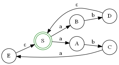
(b) Transition diagram.

Figure 4. An ndfa for L = (aba $\cup$ ab)${}^{\texttt{*}}$.

To illustrate the proposed constructor, consider the ndfa displayed in Figure 4. First, the empties for each state are computed. The following table displays the results:

state	E(state)
S	(S)
A	(A)
B	(B)
C	(C)
D	(D S)
E	(E S)

Second, the super state transition function is computed. The process starts with the only known super state, E(S), which is the start super state for the dfa. For each element, a, of the alphabet, the union of the states that can be reached from any states in E(S) by first consuming a is computed. E(S) only contains S and, thus, the following transitions are obtained:

     ((S) a (A B))
     ((S) b ())

Observe that two new needed super states have been discovered: (A B) and '() (denoting the dead state for the dfa under construction). These are added to the list of unprocessed super states. The process is repeated for each unprocessed super state. For instance, the process may continue with (A B). Both A and B can go nowhere on a a. On a b, from A the machine can transition to C and from B the machine can transition to D and by an $\epsilon$-transition to S. The needed super state transitions are:

     ((A B) a ())
     ((A B) b (C D S))

In this case, a single new super state is discovered, (C D S), and added to the list of unprocessed super states. The process continues in a similar fashion until there are no more super states to process. The following table summarizes the computed super state transition function:

Super State	a	b
(S)	(A B)	()
(A B)	()	(C D S)
(C D S)	(E S A B)	()
(E S A B)	(A B)	(C D S)
()	()	()

(define D
  (make-dfa `(S A B C ,DEAD)
            '(a b)
            'S
            '(S B C)
            `((S a A) (S b ,DEAD)
              (A a ,DEAD) (A b B)
              (B a C) (B b ,DEAD)
             (C a A) (C b B)
             (,DEAD a ,DEAD)
             (,DEAD b ,DEAD))))

;; Tests for D
(check-equal?
  (sm-testequiv? D ND 500)
  #t)
(check-equal?
  (sm-testequiv? (ndfa->dfa ND)
                 D
                 500)
  #t)

(a) Implementation.

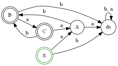
(b) Transition diagram.

Figure 5. A dfa for L = (aba $\cup$ ab)${}^{\texttt{*}}$.

To build a dfa the super states must be mapped to FSM states. The following table is one such encoding :

Super State	dfa State
(S)	S
(A B)	A
(C D S)	B
(E S A B)	C
()	DEAD

Observe that S, B, and C are final states in the dfa because the super state they represent contains the only final state in ND. This leads to the dfa displayed in Figure 5. The tests validate that the deterministic and nondeterministic implementations decide the same language. The second check-equal? uses FSM’s primitive, ndfa->dfa, to transform an ndfa to a dfa and validates that FSM’s transformation and D are equivalent.

4.3. Implementation Sketch

The implementation presented uses the following data definitions:

     ;; Data Definitions
     ;;
     ;;  An ndfa transition rule, ndfa-rule, is a
     ;;  (list state symbol state)
     ;;
     ;;  A super state, ss, is a (listof state)
     ;;
     ;;  A super state dfa rule, ss-dfa-rule, is a
     ;;  (list ss symbol ss)
     ;;
     ;;  An empties table, emps-tbl, is a
     ;;  (listof (list state ss))
     ;;
     ;;  A super state name table, ss-name-table, is a
     ;;  (listof (list ss state))

;; ndfa $\rightarrow$ dfa
;; Purpose: Convert the given ndfa to an equivalent dfa
(define (ndfa2dfa M)
 (if (eq? (sm-type M) 'dfa)
   M
   (convert (sm-states M) (sm-sigma M) (sm-start M) (sm-finals M) (sm-rules M))))

;; Tests for ndfa2dfa
(define M (ndfa2dfa AT-LEAST-ONE-MISSING))
(check-equal? (sm-testequiv? AT-LEAST-ONE-MISSING M 500) #t)
(check-equal? (sm-testequiv? M (ndfa->dfa AT-LEAST-ONE-MISSING) 500) #t)

(define N (ndfa2dfa ND))
(check-equal? (sm-testequiv? ND N 500) #t)
(check-equal? (sm-testequiv? N (ndfa->dfa ND) 500) #t)

Figure 6. The main function to convert an ndfa to a dfa.

The main function, ndfa2dfa, tests if the given machine is a dfa. If so, it returns it given that no transformation is needed. Otherwise, an auxiliary converting function is called with the components of the given ndfa. The implementation is displayed in Figure 6.

;; (listof state) alphabet state (listof state) (listof ndfa-rule) $\rightarrow$ dfa
;; Purpose: Create a dfa from the given ndfa components
(define (convert states sigma start finals rules)
  (let* [(empties (compute-empties-tbl states rules))
         (ss-dfa-rules
          (compute-ss-dfa-rules (list (extract-empties start empties))
                                sigma
                                empties
                                rules
                                '()))
         (super-states (remove-duplicates
                         (append-map ($\lambda$ (r) (list (first r) (third r)))
                                     ss-dfa-rules)))
         (ss-name-tbl (compute-ss-name-tbl super-states))]
    (make-dfa (map ($\lambda$ (ss) (second (assoc ss ss-name-tbl)))
                   super-states)
              sigma
              (second (assoc (first super-states) ss-name-tbl))
              (map ($\lambda$ (ss) (second (assoc ss ss-name-tbl)))
                   (filter ($\lambda$ (ss) (ormap ($\lambda$ (s) (member s finals)) ss))
                           super-states))
              (map ($\lambda$ (r) (list (second (assoc (first r) ss-name-tbl))
                                    (second r)
                                    (second (assoc (third r) ss-name-tbl))))
                   ss-dfa-rules)
              'no-dead)))

Figure 7. The convert implementation.

The convert function takes as input the components of an ndfa. To build a dfa it computes the following values:

1. The empties table

2. The super state transition rules

3. The super state name table

The implementation of this design is displayed in Figure 7. The functions compute-empties-tbl and compute-ss-name-tbl are used to compute, respectively, the empties table and the super states table. These functions are straightforward to implement and, in the interest of brevity, are not presented.

;; (listof ss) alphabet emps-tbl (listof ndfa-rule) (listof ss)
;; $\rightarrow$ (listof ss-dfa-rule)
;; Purpose: Compute the super state dfa rules
;; Accumulator Invariants:
;;               ssts = the super states explored
;;     to-search-ssts = the super states that must still be explored
(define (compute-ss-dfa-rules to-search-ssts sigma empties rules ssts)
      $\vdots$
 (if (empty? to-search-ssts)
     '()
     (let* [(curr-ss (first to-search-ssts))
            (reachables (find-reachables curr-ss sigma rules empties))
            (to-super-states
             (build-list (length sigma) ($\lambda$ (i) (get-reachable i reachables))))
            (new-rules (map ($\lambda$ (sst a) (list curr-ss a sst))
                            to-super-states
                            sigma))]
       (append
         new-rules
         (compute-ss-dfa-rules
           (append (rest to-search-ssts)
                   (filter ($\lambda$ (ss)
                             (not (member ss (append to-search-ssts ssts))))
                           to-super-states))
           sigma
           empties
           rules
           (cons curr-ss ssts))))))

Figure 8. Function to compute the super state transition function.

To compute the super state transition function we perform a breadth-first search rooted at the super states that still need to be explored to identify transition rules. There are two accumulators: one for the super states left to explore and one for the super states already explored. If there are no states left to explore, the empty list is returned because the search for super state dfa rules is done. Otherwise, the first unexplored super state, denoted curr-ss, is processed. The set of reachable states for every state in the first unexplored super state, consuming every element of the alphabet, is computed. For instance, if the first unexplored super state is '(A B C) and the alphabet is '(a b) then the reachable states have the following structure:

     (((reachable from A on a) (reachable from A on b))
      ((reachable from B on a) (reachable from B on b))
      ((reachable from C on a) (reachable from C on b)))

There are three sublists in the list: one for each state in the first unexplored super state. Each sublist has a list of states that are reachable for each element of the alphabet. From this, the super states to transition into, to-super-states, are computed. For instance, the super state reachable on an a is formed by all the states reachable on an a from A, B, and C (without repetitions). The dfa transition rules are generated by simultaneously traversing to-super-states and the alphabet. Assuming a is the current alphabet element and sst is the current element of to-super-states during such a traversal, then a super state dfa rule of the following form is created: (curr-ss a sst). Finally, the super state dfa rules generated are appended with the result of recursively processing a new accumulator for unexplored super states containing the rest of the said accumulator and any new super states generated for the new rules, the same alphabet, the same empties table, the same list of ndfa rules, and a new accumulator for explored states obtained by adding the first unexplored super state. The compute-ss-dfa-rules function based on this design is displayed in Figure 8. This is the bulk of what is needed to compute the super state dfa transition function. The remaining auxiliary functions are straightforward and not further discussed.

5. Visualization in FSM

To visualize the ndfa to dfa transformation, two state diagrams are built at every step. The first is for the ndfa and is used to highlight the edges that have been used in the construction of the dfa. The second is for the dfa that is built piecemeal one edge at a time.

5.1. Design Idea

The ndfa is denoted by N and the dfa is denoted by D. The transition diagram for N is always fully displayed. The transition diagram for D is built one transition at a time. The user may step forwards or backwards in the computation one step at the time. In addition, the user may have the dfa’s transition diagram completed in one step.

The ndfa’s edges are partitioned into three subsets that are color coded. The first is the set of edges that have not yet been used in the dfa’s construction. These edges are drawn in black and are referred to as bledges. The second is the set of edges used to add the latest dfa edge. These edges are highlighted in violet and are referred to as hedges. Finally, the third set is for edges that have previously been used in the dfa construction. These edges are faded out in gray and are referred to as fedges.

The state transition diagram is built using the output of compute-ss-dfa-rules. The dfa super state transitions are partitioned into two sets. The first contains the super state transitions that have been processed in the construction and are denoted as ad-edges. The second contains the super state transitions that are unprocessed and are denoted by up-edges. In addition, the super states included in the constructed part of the dfa are accumulated to prevent adding any given super state more than once.

Initially, D’s transition diagram only contains E(s), where s is N’s starting state. In N’s transition diagram, initially, the $\epsilon$-transitions on any path from s to any state in E(s) are hedges and all other edges are bledges. Every time the user moves the computation forward, the next element of up-edges, (SS₁ a SS₂), is processed and added to ad-edges resulting in a new edge appearing in the dfa’s transition diagram. Simultaneously, the hedges are added to the fedges to have them faded. In addition, the new set of hedges and the new set of bledges are computed. The new set of hedges contains all edges in N that consume a from any state in SS₁ and all the $\epsilon$-transitions that are reachable from any state in SS₁ after consuming the a. The new set of bledges is obtained by removing the new hedges from it. Finally, SS₂ is added, if not already present, to the accumulator for super states that are part of the dfa constructed thus far.

Every time the user moves the computation backwards, the process above is reversed. The last edge added is removed from D’s transition diagram. That is, the newest element in ad-edges is moved to up-edges. The next newest element in ad-edges is used to compute the new sets of hedges, fedges, and bledges as described above. If necessary, the newest element in the super state accumulator is removed.

Finally, when the user moves to complete the ndfa transformation, all the up-edges are processed as described above. In this manner, the user may still step backwards in the computation if she desires.

5.2. Illustrative Example

(define aa-ab
  (make-ndfa
    '(S A B F)
    '(a b)
    'S
    '(A B)
    `((S a A)
      (S a B)
      (S ,EMP F)
      (A a A)
      (B b B))))

(a) Implementation.

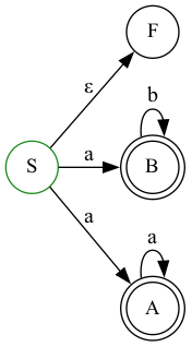
(b) Transition diagram.

Figure 9. An ndfa for L = L={$\epsilon\cup aa^{\texttt{*}}\cup ab^{\texttt{*}}$}

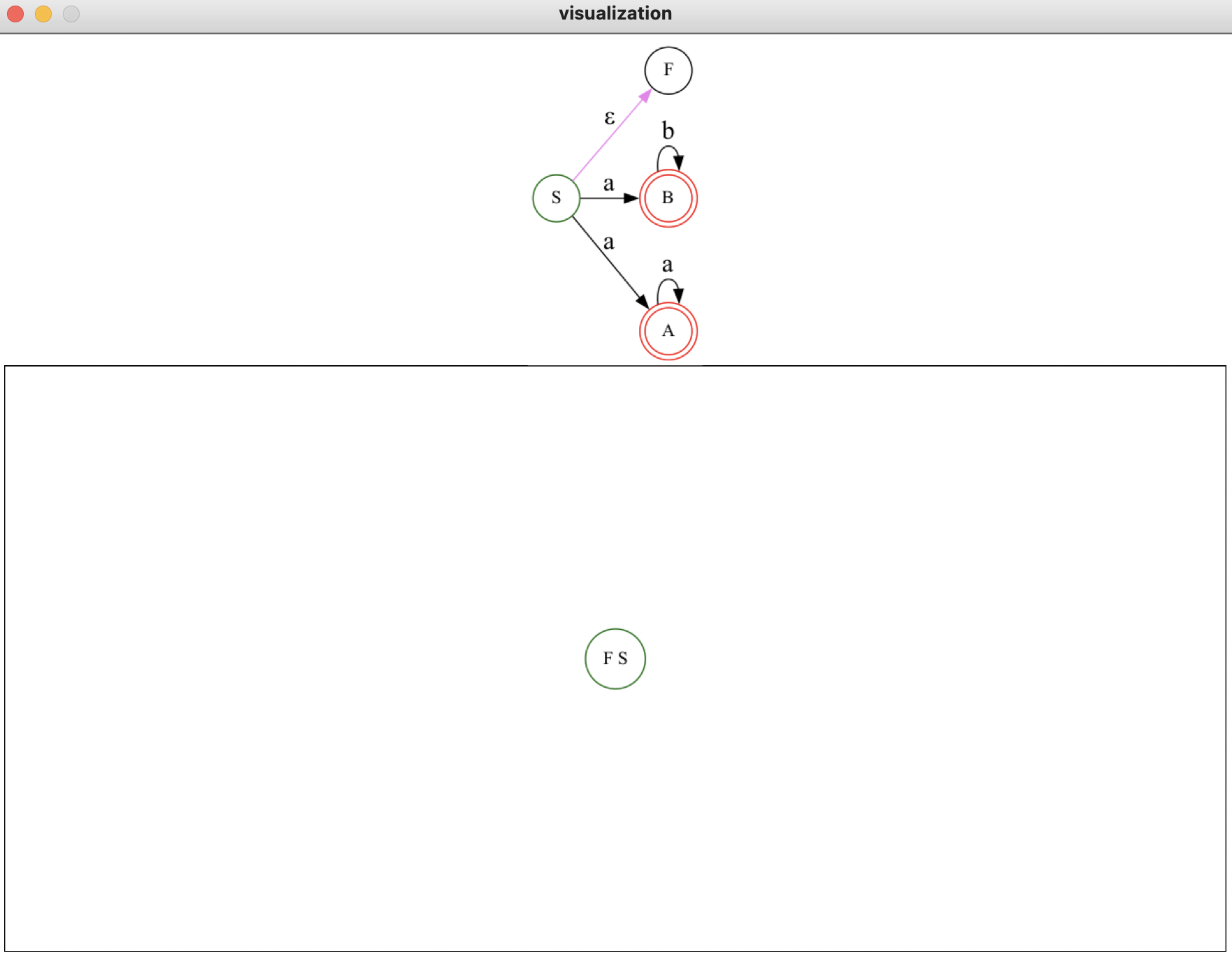
Figure 10. The initial visualization state.

To illustrate the transformation, consider the ndfa defined and its transition diagram in Figure 9. Initially, the diagram for the dfa only contains one super state for E(S)=(F S). The diagram for the ndfa only has one hedge from S to F, because (S $\epsilon$ F) is the only edge used so far in the dfa’s construction. All other edges in the ndfa’s diagram are bledges. This initial state of the visualization is displayed in Figure 10.

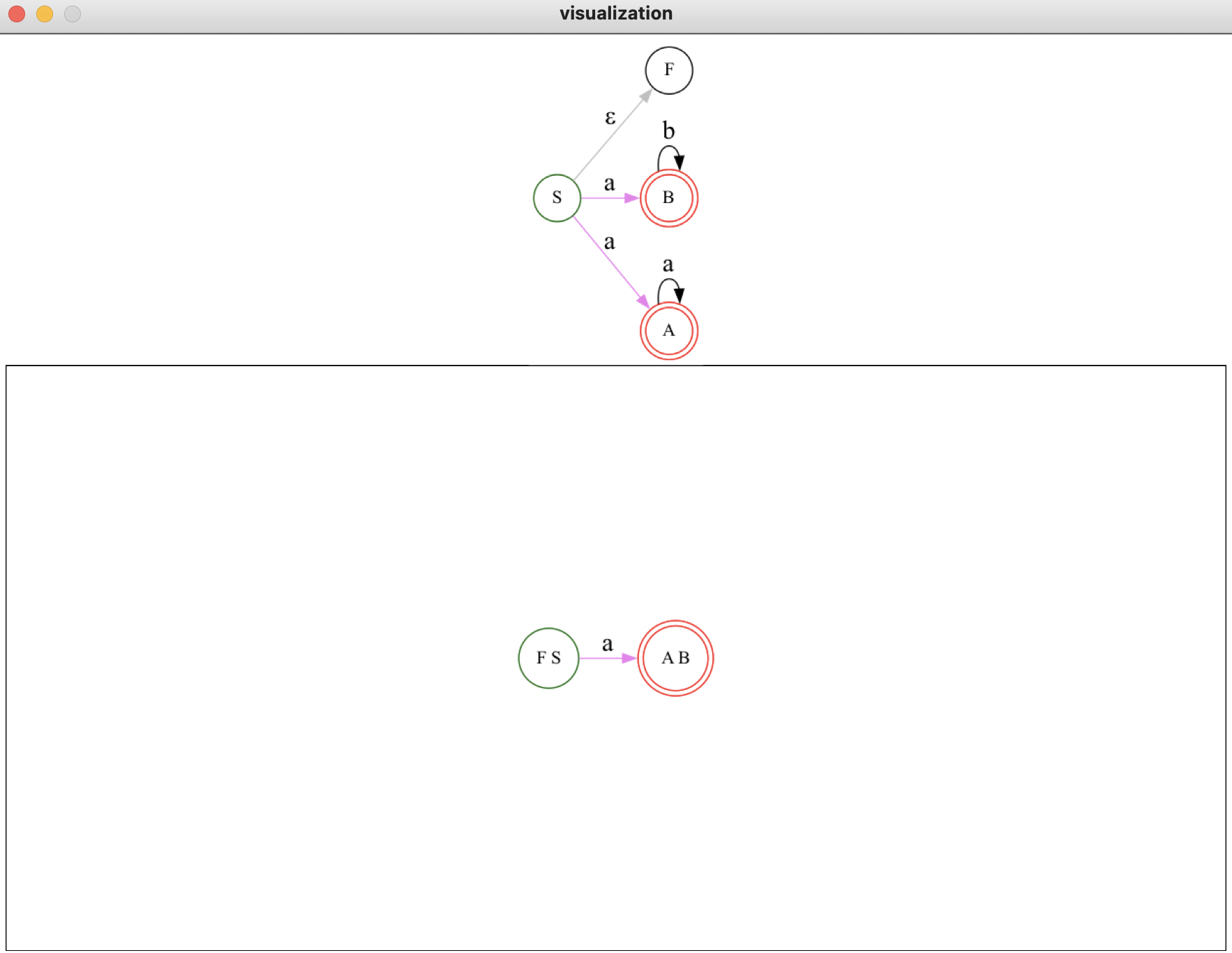
Figure 11. The visualization state after moving the visualization one step forward.

When the user moves one step forward in the computation, the simulation adds ((F S) a (A B)) to the dfa. It is highlighted in violet as it is the last dfa edge added. In the ndfa’s diagram, the $\epsilon$-transition from S to F becomes a fedge and, thus, is highlighted in gray. In addition, all reachable edges out of S on an a are part of the dfa’s transition and, thus, are hedges highlighted in violet. All other ndfa edges are bledges rendered in black. Observe that the user can easily determine why there is a dfa super state (A B). Its existence follows from the hedges highlighted in violet in the ndfa. These hedges define all the states reachable from S on an a.

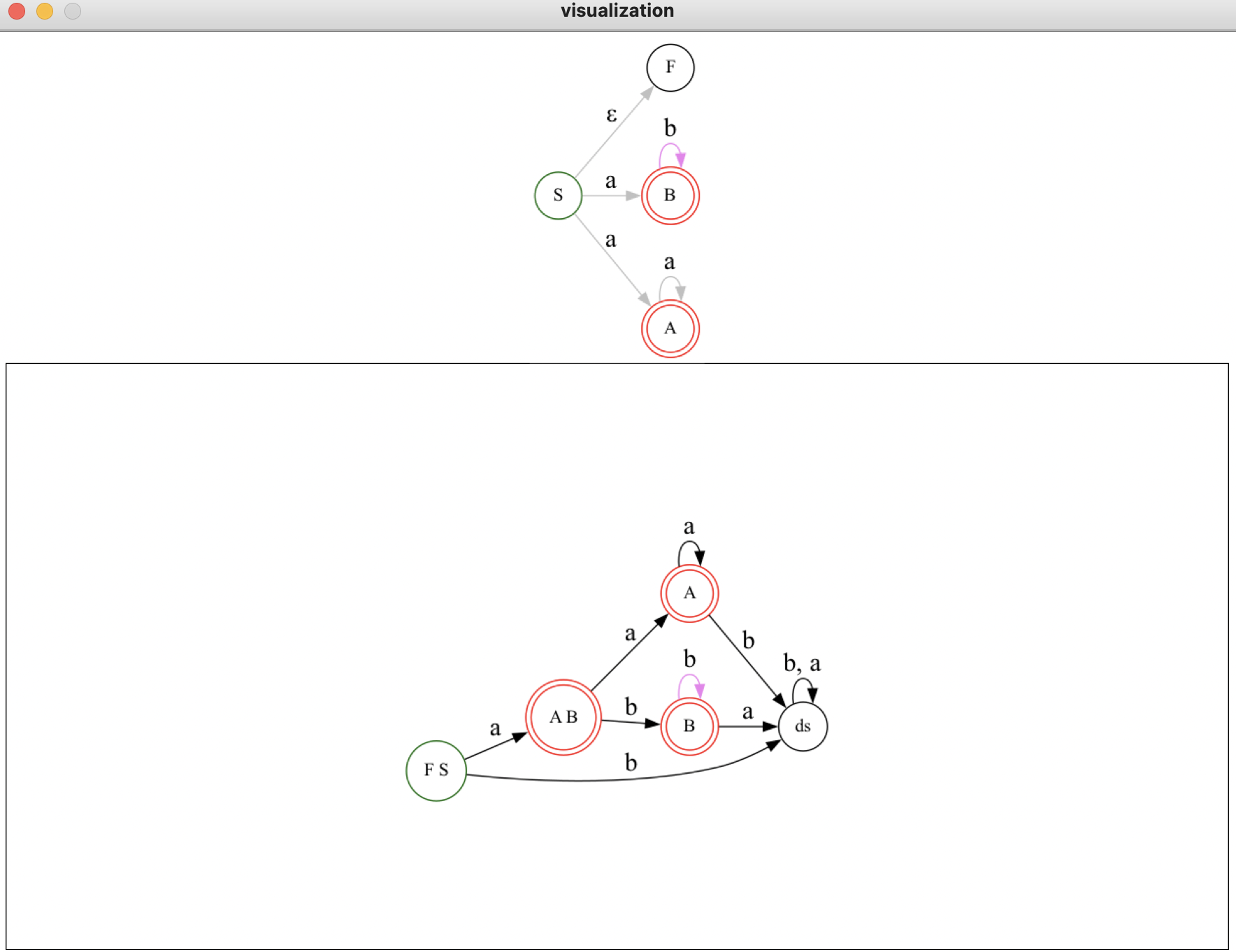
Figure 12. The final visualization state.

If the user completes the computation in one step, all the dfa edges are rendered. The dfa transition diagram is generated by processing all the super state transitions in the same order as if the user stepped through the computation. Therefore, the dfa edge for the last super state transition processed is highlighted in violet. This is depicted in the finalized dfa transition diagram in Figure 12. In the diagram for the ndfa, only (B b B) is a hedge given that the only state reachable from B on a b is B. Observe that this clearly explains why there is a dfa super state that only contains B. The reader can compare the dfa transition diagram in Figure 12 with the transition diagrams in Figure 1(b) and Figure 2(b) obtained using, respectively, JFLAP and OpenFLAP. FSM’s use of GraphViz results in superior renderings for dfa transition diagrams.

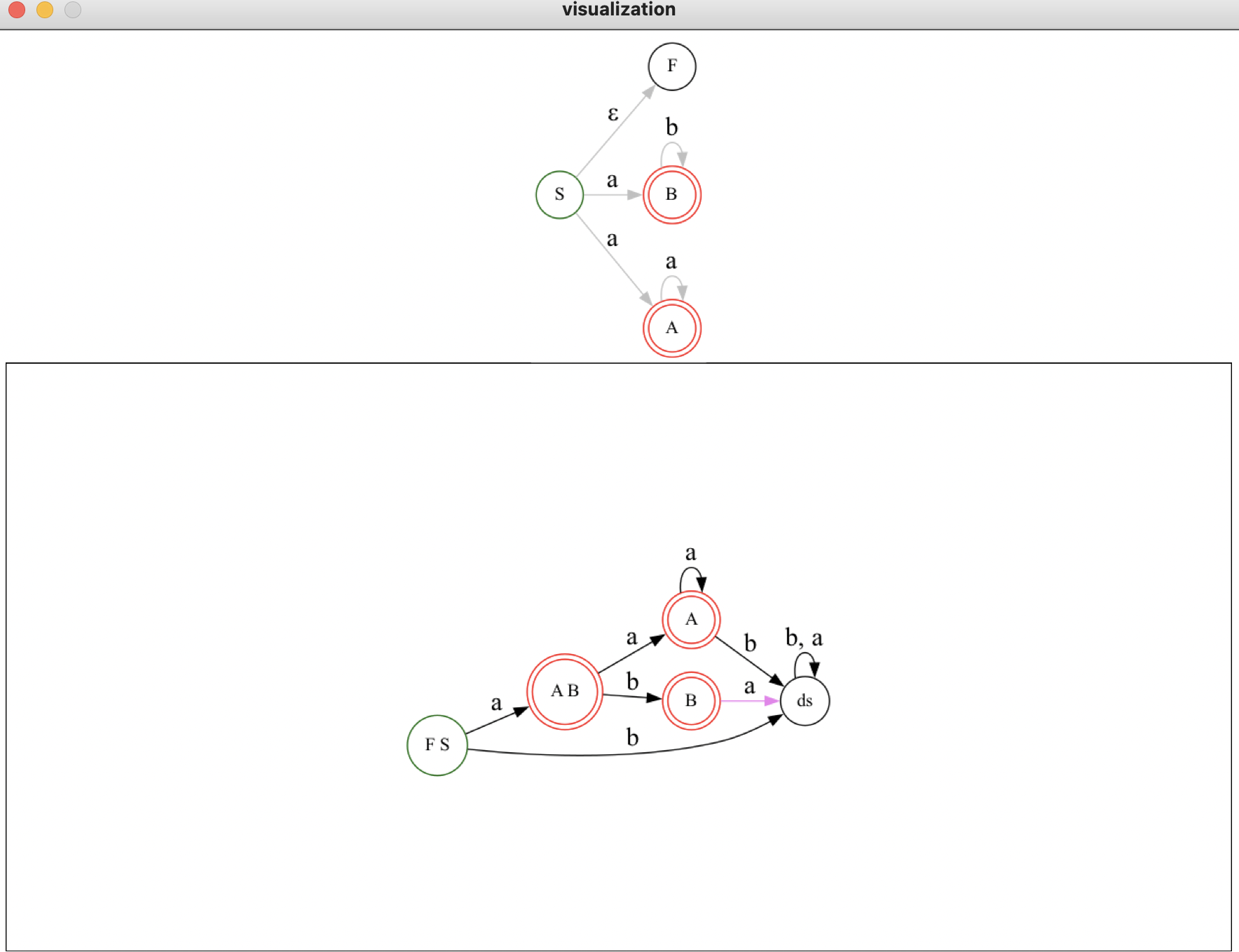
Figure 13. The visualization state after moving the computation one step backwards.

Finally, we illustrate what happens when the user takes a step backwards in the computation. The last edge added to the dfa’s diagram is removed, making the next-to-last dfa edge added the last edge added in the new state of the computation. For the ndfa, the current hedges are made bledges and, thus, are no longer highlighted. In addition, the hedges that existed when the next-to-last dfa edge was added are recomputed and removed from fedges. For instance, if the user moves one step backwards in the computation’s state displayed in Figure 12, the dfa edge (B b B) is removed and the next-to-last dfa edge added, (B a ds), is highlighted. In the ndfa (B b B) becomes a fedge. This is correct because this edge is part of the dfa construction given the super state edge ((A B) b B). This illustrates that multiple ndfa transitions end up in the same super state, thus, removing an edge from the dfa diagram does not automatically remove an edge from the ndfa diagram. Sometimes an ndfa edge is moved to a different subset of the ndfa-edges partition. To close, we note that when the last dfa edge added is to the fresh dead state then there are no hedges in the ndfa given that this state is not part of the ndfa.

5.3. Implementation Highlights

The state of the visualization is represented using a structure:

   (struct viz-state (up-edges ad-edges incl-nodes M hedges fedges bledges))

The first three fields are for the state of the dfa under construction described as follows:

up-edges::

the unprocessed dfa edges

ad-edges::

the processed dfa edges

incl-nodes::

the super states appearing in ad-edges

The fourth field is the given ndfa. The last three fields represent the partition of ndfa edges described as follows:

hedges::

the most recent ndfa edges processed that are rendered in violet

fedges::

the previous ndfa edges processed that are rendered in gray

bledges::

the unprocessed ndfa that are rendered in black

At the beginning of the visualization, all the dfa edges are unprocessed. The only super state rendered for the dfa is the starting super state. For the ndfa, the set of hedges contains all ndfa edges reachable on $\epsilon$-transitions from any state in the starting super state, the set of fedges is empty (i.e., there are no previously processed ndfa edges), and the set of bledges are all the ndfa edges that are not a hedges. Thus, the initial viz-state value is defined as follows:

  (let* [(ss-edges (compute-ss-edges M))
         (super-start-state
           (compute-empties (list (sm-start M)) (sm-rules M) '()))
         (init-hedges (compute-all-hedges (sm-rules M) super-start-state '()))
    (viz-state ss-edges
               '()
               (list super-start-state)
               M
               init-hedges
               '()
               (remove init-hedges (sm-rules M)))

Here, compute-ss-edges returns the super state dfa edges given an ndfa, compute-empties returns the empties of the given state, and compute-all-hedges returns the set of hedges for the given super state and the given dfa super state edge added. In this case, '() is given as the edge added because there is no dfa edge being added.

Moving the computation forward means that the next super state dfa edge is processed. Therefore, the current dfa super state edge (i.e., the first unprocessed) is moved to the set of processed dfa super state edges. Any super states in the first unprocessed dfa edge, if not already included, are added to incl-nodes. For the ndfa, the new set of hedges is computed using the current dfa rule’s destination super state. To compute the new set of fedges, two cases are distinguished. When the new set of unprocessed dfa super state edges is empty, the computation can no longer move forward. In order for the simulation to properly move backwards, the new hedges are added to the fedges. This is consistent with the design, because for edge rendering hedges take precedence over fedges. Thus, the rendering of the dfa remains correct. When the new set of unprocessed dfa super state edges is not empty, the existing hedges are added to the set of fedges. Finally, the new set of bledges is obtained by removing the new hedges. This design is implemented as follows:

(let* [(curr-dfa-ss-edge (first (viz-state-up-edges a-viz-state)))
       (new-up-edges (rest (viz-state-up-edges a-viz-state)))
       (new-ad-edges (cons curr-dfa-ss-edge (viz-state-ad-edges a-viz-state)))
       (new-incl-nodes
         (add-included-node (viz-state-incl-nodes a-viz-state)
         curr-dfa-ss-edge))
       (new-hedges (compute-all-hedges (sm-rules (viz-state-M a-viz-state))
                                       (third curr-dfa-ss-edge)
                                       curr-dfa-ss-edge))
       (new-fedges (if (empty? new-up-edges)
                       (append new-hedges (viz-state-fedges a-viz-state))
                       (append (viz-state-hedges a-viz-state)
                               (viz-state-fedges a-viz-state))))
       (new-bledges (remove-edges new-hedges (viz-state-bledges a-viz-state)))]
  (viz-state new-up-edges
             new-ad-edges
             new-incl-nodes
             (viz-state-M a-viz-state)
             new-hedges
             new-fedges
             new-bledges))

Moving the computation backwards means that the last processed dfa super state edge is moved to the set of unprocessed dfa super state edges. If necessary, the last processed dfa edge’s destination state is removed from incl-nodes. For the new hedges set, two cases are distinguished. When the set of processed dfa super state edges is empty, the visualization is at the beginning. In this case, the new set of hedges is computed using the dfa’s starting super state. Otherwise, the new set of hedges is computed using the first dfa super state edge in the new set of processed edges. For the new set of fedges, two cases are also distinguished. If the new set of processed edges is empty, then there are no fedges. Otherwise, the new fedges are obtained by removing the hedges computed using the destination state of the last dfa super state edge processed. Finally, the set of new bledges is given by appending the hedges computed using the destination state of the last dfa super state edge processed and the set of bledges. This design is implemented as follows:

(let* [(last-dfa-pedge (first (viz-state-ad-edges a-viz-state)))
       (new-up-edges (cons last-dfa-pedge (viz-state-up-edges a-viz-state)))
       (new-ad-edges (rest (viz-state-ad-edges a-viz-state)))
       (new-incl-nodes (remove-included-node (viz-state-incl-nodes a-viz-state)
                                             last-dfa-pedge
                                             new-ad-edges))
       (new-hedges (if (empty? new-ad-edges)
                       (compute-all-hedges
                          (sm-rules (viz-state-M a-viz-state))
                          (compute-empties
                            (list (sm-start (viz-state-M a-viz-state)))
                            (sm-rules (viz-state-M a-viz-state))
                            '())
                          '())
                       (compute-all-hedges (sm-rules (viz-state-M a-viz-state))
                                           (third (first new-ad-edges))
                                           (first new-ad-edges))))
       (prev-hedges (compute-all-hedges (sm-rules (viz-state-M a-viz-state))
                                            (third last-dfa-pedge)
                                            last-dfa-pedge))
       (new-fedges (if (empty? new-ad-edges)
                       empty
                       (remove-edges prev-hedges
                                     (viz-state-fedges a-viz-state))))
       (new-bledges (remove-duplicates
                      (append prev-hedges
                              (viz-state-bledges a-viz-state))))]
  (make-world new-up-edges
              new-ad-edges
              new-incl-nodes
              (viz-state-M a-viz-state)
              new-hedges
              new-fedges
              new-bledges))

Finally, when the visualization is moved to its final state all dfa super state edges are processed and all super states are in incl-nodes. The new set of hedges is computed using the destination super state of the last dfa edge processed. The new set of fedges is obtained by appending the hedges in the same order as added by moving the visualization forward in a piecemeal fashion and the hedges associated with the starting super state. Finally, the new set of bledges is empty. This design is implemented as follows:

(let* [(ss-edges (append (reverse (viz-state-ad-edges a-viz-state))
                         (viz-state-up-edges a-viz-state))))
       (super-start-state (first (first ss-edges)))
       (new-up-edges '())
       (new-ad-edges (reverse ss-edges))
       (new-incl-nodes
         (remove-duplicates (append-map ($\lambda$ (e) (list (first e) (third e)))
                                        new-ad-edges)))
       (new-hedges (compute-all-hedges (sm-rules (viz-state-M a-viz-state))
                                       (third (first new-ad-edges))
                                       (first new-ad-edges)))
       (new-fedges
         (append (compute-down-fedges (sm-rules (viz-state-M a-viz-state))
                 new-ad-edges)
                 (compute-all-hedges (sm-rules (viz-state-M a-viz-state))
                                     super-start-state
                                     '())))
       (new-bledges '())]
  (make-world new-up-edges
              new-ad-edges
              new-incl-nodes
              (viz-state-M a-viz-state)
              new-hedges
              new-fedges
              new-bledges))

6. Concluding Remarks

This article presents a novel visualization tool for the transformation of an ndfa to a dfa. The visualization simultaneously renders the ndfa’s transition diagram and the transition diagram for the dfa constructed so far. It improves the current state-of-the-art by rendering transition diagrams in an appealing manner. In addition, the last dfa edge added is highlighted as well as the corresponding ndfa edges. The ndfa edges that are already part of the dfa construction are faded out in gray and ndfa edges that are not part of the dfa construction are rendered in black. In this manner, any user can easily determine why the dfa’s super states exist, see how all ndfa edges are processed, and comprehend the development of the dfa’s transition function. The FSM visualization, unlike other visualization tools for this transformation, may be advanced both forward and backwards. Finally, the dfa’s transition diagram may be rendered in one step without preventing the user from moving the simulation backwards.

Future work includes adding visualization tools for other machine transformations or constructors. The targeted transformations include dfa to regular expression and vice versa. The targeted constructors include the closure properties under union, concatenation, Kleene star, complement, and intersection. In addition, empirical studies will be performed to collect student feedback on the work presented in this article.

References

- (1)
- Baase (1988) S. Baase. 1988. Computer Algorithms: Introduction to Design and Analysis. Addison-Wesley Publishing Company.
- Farhanaaz and Sanju (2016) Farhanaaz and V. Sanju. 2016. An Exploration on Lexical Analysis. In 2016 International Conference on Electrical, Electronics, and Optimization Techniques (ICEEOT). 253–258. https://doi.org/10.1109/ICEEOT.2016.7755127
- Gansner and North (2000) Emden R. Gansner and Stephen C. North. 2000. An Open Graph Visualization System and Its Applications to Software Engineering. Softw. Pract. Exper. 30, 11 (September 2000), 1203–1233. https://doi.org/10.1002/1097-024X(200009)30:11<1203::AID-SPE338>3.0.CO;2-N
- Gheorghe et al. (2010) Marian Gheorghe, Florentin Ipate, and Ciprian Dragomir. 2010. Formal Verification and Testing Based on P Systems. In Membrane Computing, Gheorghe Păun, Mario J. Pérez-Jiménez, Agustín Riscos-Núñez, Grzegorz Rozenberg, and Arto Salomaa (Eds.). Springer Berlin Heidelberg, Berlin, Heidelberg, 54–65.
- Gurari (1989) Eitan M. Gurari. 1989. An Introduction to the Theory of Computation. Computer Science Press.
- Hládek et al. (2020) Daniel Hládek, Ján Staš, and Matúš Pleva. 2020. Survey of Automatic Spelling Correction. Electronics 9, 10 (2020). https://doi.org/10.3390/electronics9101670
- Hopcroft et al. (2006) John E. Hopcroft, Rajeev Motwani, and Jeffrey D. Ullman. 2006. Introduction to Automata Theory, Languages, and Computation (3rd Edition). Addison-Wesley Longman Publishing Co., Inc., USA.
- Ilgun et al. (1995) Koral Ilgun, R. A. Kemmerer, and Phillip A. Porras. 1995. State Transition Analysis: A Rule-Based Intrusion Detection Approach. IEEE Trans. Softw. Eng. 21, 3 (March 1995), 181–199. https://doi.org/10.1109/32.372146
- Lewis and Papadimitriou (1997) Harry R. Lewis and Christos H. Papadimitriou. 1997. Elements of the Theory of Computation (2nd ed.). Prentice Hall PTR, Upper Saddle River, NJ, USA. https://doi.org/10.1145/300307.1040360
- Martin (2003) John C. Martin. 2003. Introduction to Languages and the Theory of Computation (3 ed.). McGraw-Hill, Inc., New York, NY, USA.
- Mohammed (2020) Mostafa Kamel Osman Mohammed. 2020. Teaching Formal Languages through Visualizations, Simulators, Auto-graded Exercises, and Programmed Instruction. In Proceedings of the 51st ACM Technical Symposium on Computer Science Education, SIGCSE 2020, Portland, OR, USA, March 11-14, 2020, Jian Zhang, Mark Sherriff, Sarah Heckman, Pamela A. Cutter, and Alvaro E. Monge (Eds.). ACM, 1429. https://doi.org/10.1145/3328778.3372711
- Morazán and Antunez (2014) Marco T. Morazán and Rosario Antunez. 2014. Functional Automata - Formal Languages for Computer Science Students. In Proceedings 3rd International Workshop on Trends in Functional Programming in Education, TFPIE 2014, Soesterberg, The Netherlands, 25th May 2014 (EPTCS, Vol. 170), James L. Caldwell, Philip K. F. Hölzenspies, and Peter Achten (Eds.). 19–32. https://doi.org/10.4204/EPTCS.170.2
- Morazán et al. (2020) Marco T. Morazán, Joshua M. Schappel, and Sachin Mahashabde. 2020. Visual Designing and Debugging of Deterministic Finite-State Machines in FSM. Electronic Proceedings in Theoretical Computer Science 321 (August 2020), 55–77. https://doi.org/10.4204/eptcs.321.4
- Parsons (1992) Thomas W. Parsons. 1992. Introduction to Compiler Construction. Computer Science Press, Inc., USA.
- Prithi and Sumathi (2020) S. Prithi and S. Sumathi. 2020. LD2FA-PSO: A novel Learning Dynamic Deterministic Finite Automata with PSO Algorithm for Secured Energy Efficient Routing in Wireless Sensor Network. Ad Hoc Networks 97 (2020), 102024. https://doi.org/10.1016/j.adhoc.2019.102024
- Rich (2019) Elaine Rich. 2019. Automata, Computability and Complexity: Theory and Applications. Pearson Prentice Hall.
- Rodger (2006) Susan H. Rodger. 2006. JFLAP: An Interactive Formal Languages and Automata Package. Jones and Bartlett Publishers, Inc., USA.
- Rodger et al. (2006) Susan H. Rodger, Bart Bressler, Thomas Finley, and Stephen Reading. 2006. Turning automata theory into a hands-on course. In Proceedings of the 37th SIGCSE Technical Symposium on Computer Science Education, SIGCSE 2006, Houston, Texas, USA, March 3-5, 2006, Doug Baldwin, Paul T. Tymann, Susan M. Haller, and Ingrid Russell (Eds.). ACM, 379–383. https://doi.org/10.1145/1121341.1121459
- Sipser (2013) Michael Sipser. 2013. Introduction to the Theory of Computation (3rd ed.). Cengage Learning.