Generalized Riemann Problem Method for the Kapila Model of Compressible Multiphase Flows I: Temporal-Spatial Coupling Finite Volume Scheme

Abstract

A second-order accurate and robust numerical scheme is developed for the Kapila model to simulate compressible multiphase flows. The scheme is formulated within the temporal-spatial coupling framework with the generalized Riemann problem (GRP) solver applied as the cornerstone. The use of the GRP solver enhances the capability of the resulting scheme to handle the stiffness of the Kapila model in two ways. Firstly, in addition to Riemann solutions, the time derivatives of flow variables at cell interfaces are obtained by the GRP solver. The coupled values, i.e. Riemann solutions and time derivatives, lead to a straightforward approximation to the velocity divergence at the next time level, enabling a semi-implicit time discretization to the volume fraction equation. Secondly, the use of time derivatives enables numerical fluxes to comprehensively account for the effect of the source term, which includes interactions between phases. The robustness of the resulting numerical scheme is therefore further improved. Several challenging numerical experiments are conducted to demonstrate the performance of the proposed finite volume scheme. In particular, a test case with a nonlinear smooth solution is designed to verify the numerical accuracy.

[aff-iapcm]organization=Institute of Applied Physics and Computational Mathematics,postcode=100094, city=Beijing, country=China

1 Introduction

Compressible multiphase flows appear in numerous scientific and engineering disciplines, including astrophysics [20, 1, 32], inertial confinement fusion [25, 10, 41], cavitation flows [27, 47, 38], deflagration-to-detonation transitions [44, 9, 39]. There has been an enormous amount of successful applications of sharp interface methods in numerical simulations involving compressible multiphase flows [50, 17, 8, 15]. In contrast, this work concentrates on the development of a shock-capturing scheme that is capable of capturing interfaces between pure fluids as well as fluid mixtures. To achieve this, the Kapila model is employed in the present work for its capability of effectively modeling the underlying physical process of compressible multiphase flows [22, 21, 46].

We first have a brief overview of the development of mathematical models for compressible multiphase flows. In [4], Baer and Nunziato proposed a seven-equation model to describe the dynamics of multiphase flows, specifically in solid granular explosives mixed with gaseous products, which is commonly referred to as the Baer-Nunziato (BN) model. The BN model includes mass, momentum, and energy balance laws for each individual phase. The six governing equations are augmented by a seventh one modeling the gaseous volume fraction evolution. After being further extended to model general multiphase flows [42], much attention has been devoted to develop numerical schemes for the seven-equation model [2, 3, 49, 23, 29]. However, the presence of the non-conservative product in the seven-equation model complicates the design of numerical schemes and makes the uniqueness of the Riemann solution uncertain [11]. This motivates the study of a simplified model. By performing asymptotic analysis towards the limit of velocity and pressure equilibria, a single-velocity and single-pressure model of compressible multiphase flows was derived [21]. This model, termed as the Kapila model or the five-equation reduced model, is composed of continuity equations of each phase, conservation laws of the total momentum and the total energy, and the volume fraction equation with a stiff source term that accounts for the interaction between phases. The sound speed of the mixture is defined by the Wood formula [53]. The same five-equation model was also derived in [34]. Although this model was derived from the seven-equation model for mixtures, it can be applied to numerical simulations of interfaces separating either pure fluids or fluid mixtures [46].

After its introduction, the Kapila model has been widely used in numerical simulations of compressible multiphase flows [36, 24, 51]. Nevertheless, such efforts face two distinct difficulties. In the first place, the stiffness of the source term in the volume fraction equation, which arises as the result of the stiff limit of the relaxation process in the original seven-equation model, is particularly difficult to approximate and makes keeping the boundedness of the volume fraction a challenging task. Secondly, the non-monotonic behavior of the Wood sound speed in relation to volume fractions leads to Mach number oscillations in the numerical diffusion zone of an interface. To mitigate these difficulties, Saurel et al. proposed a projection-relaxation scheme [43, 37], which relies on resolving subcell structures of the numerical solution. Later, this method was further enhanced by relaxing the pressure equilibrium assumption [48].

This work provides an alternative approach to address the stiffness of the Kapila model. To accomplish this, we highlight the significance of the temporal-spatial coupling framework to develop high-resolution and robust numerical schemes for compressible fluid flows [30]. In practical implementations, Lax-Wendroff type flux solvers, among which the generalized Riemann problem (GRP) solver is regarded as a typical representative, are applied as the cornerstone. The generalized Riemann problem is formulated as the initial value problem (IVP) of hyperbolic partial differential equations (PDEs) with piecewise smooth initial data in place of piecewise constant ones in the Riemann problem. The GRP solver was initially proposed in the context of gas dynamics [5, 6], and a more straightforward and efficient version of the GRP solver was later developed in the Eulerian framework [7]. Under the acoustic assumption, the GRP can be linearized and thus solved approximately [33, 52, 14, 35].

In comparison with the Riemann problem, the GRP features waves emanating from the initial discontinuity that no longer travel along straight lines, and provides instantaneous time derivatives of flow variables along with Riemann solutions. The fundamental approach adopted to solve the GRP involves the so-called Lax-Wendroff procedure [26], which employs governing equations to quantify the relation between the time derivative of the solution and its initial spatial variation [30]. The coupled values, i.e. Riemann solutions and instantaneous time derivatives, play a vital role in implementations of temporal-spatial coupling numerical schemes, enabling evolutionary interface values of flow variables. This feature has been successfully used to develop compact data reconstructions, which rely on approximating gradients of flow variables at the next time level [13, 18, 19]. Additionally, it is illustrated that time derivatives incorporate the transversal effect of the flow field into numerical fluxes, which facilitates an accurate resolution to multi-dimensional effects in numerical computations [28].

Regarding the Kapila model, the temporal-spatial coupling framework enhances the robustness of the numerical scheme in two ways. The first notable advantage is that the source term in the volume fraction equation can be evolved using a semi-implicit discretization. This is possible since one can approximate the velocity divergence at the next time level, as done in compact data reconstructions [13, 18, 19]. When specifically implementing the Crank-Nicolson evolution, a time step restriction to preserve the boundedness of volume fractions can be established. Secondly, thanks to the Lax-Wendroff procedure which makes thorough use of governing PDEs, the compression or expansion effect carried by the source term in the volume fraction equation is fully resolved by utilizing time derivatives at cell interfaces. As a result, the capability of numerical fluxes to capture interactions between phases is considerably improved.

It is worth to mention that in the presence of strong nonlinear waves, the nonlinear GRP solver is imperative since it effectively resolves essential thermodynamical information regarding the evolution of the flow field, as demonstrated in the context of compressible single-material flow simulations [31]. This feature is of particular importance in multiphase flow simulations involving large pressure and density ratios. To keep the conciseness of this paper, we left this topic to a separate study in [12].

This paper is organized as follows. The temporal-spatial coupling finite volume scheme for the Kapila model is constructed in Section 2. In addition, the time step restriction to preserve the boundedness of volume fractions is established therein. The corresponding GRP solver is developed in Section 3. Finally, we present results of several numerical experiments in Section 4 to demonstrate the performance of the proposed scheme. Several concluding remarks are put in Section 5.

2 Finite Volume Scheme for the Kapila Model

This section is dedicated to the development of a finite volume scheme for the Kapila model. In two-phase cases, the governing equations of the Kapila model are

$$\displaystyle{\frac{\partial\zeta_{1}\rho}{\partial t}}+\nabla\cdot(\zeta_{1}\rho\mathbf{u})=0,$$ (1a)

$$\displaystyle{\frac{\partial\rho}{\partial t}}+\nabla\cdot(\rho\mathbf{u})=0,$$ (1b)

$$\displaystyle{\frac{\partial\rho\mathbf{u}}{\partial t}}+\nabla\cdot(\rho\mathbf{u}\otimes\mathbf{u})+\nabla p=0,$$ (1c)

$$\displaystyle{\frac{\partial\rho E}{\partial t}}+\nabla\cdot[(\rho E+p)\mathbf{u}]=0,$$ (1d)

$$\displaystyle{\frac{\partial\alpha_{1}}{\partial t}}+\mathbf{u}\cdot\nabla\alpha_{1}=-\alpha_{1}\alpha_{2}\displaystyle{\frac{\rho_{1}{c_{1}}^{2}-\rho_{2}{c_{2}}^{2}}{\alpha_{1}\rho_{2}{c_{2}}^{2}+\alpha_{2}\rho_{1}{c_{1}}^{2}}}\nabla\cdot\mathbf{u},$$ (1e)

where $\rho$ is the mixture density, $E$ is the total energy per unit mass, $p$ is the pressure, and $\mathbf{u}$ is the velocity. In two space dimensions, $\mathbf{u}=(u,v)^{\top}$. For each phase $k$, $\alpha_{k}$ and $\zeta_{k}$ represent the volume and mass fractions, satisfying

$$\alpha_{1}+\alpha_{2}=1,\ \ \zeta_{1}+\zeta_{2}=1.$$ (2)

Note that the continuity equation of one of the two phases is replaced by the conservation law of the mixture mass (1b). The phase density $\rho_{k}$ is defined by

$$\rho_{k}=\displaystyle{\frac{\zeta_{k}}{\alpha_{k}}}\rho,$$

which leads to $\rho=\alpha_{1}\rho_{1}+\alpha_{2}\rho_{2}$. The sound speed of each phase $k$ is defined as

$${c_{k}}^{2}=\left(\displaystyle{\frac{\partial p}{\partial\rho_{k}}}\right)_{s_{k}},$$

where $s_{k}$ is the entropy. The mixture sound speed is defined by the Wood formula [53] as

$${\frac{1}{\rho c^{2}}}=\displaystyle{\frac{\alpha_{1}}{\rho_{1}{c_{1}}^{2}}}+\displaystyle{\frac{\alpha_{2}}{\rho_{2}{c_{2}}^{2}}}.$$ (3)

The total energy of the mixture is

$$E=\displaystyle{\frac{1}{2}}\left|\mathbf{u}\right|^{2}+e,$$ (4)

where $e$ is the specific internal energy of the mixture. The thermodynamical variables of each phase follow its Gibbs relation

$$de_{k}=T_{k}ds_{k}-pd\tau_{k},$$ (5)

where $e_{k}$ and $T_{k}$ are the specific internal energy and the temperature of each phase $k$ and $\tau_{k}=\frac{1}{\rho_{k}}$ is the specific volume. From Gibbs relation (5), the specific internal energy of each phase depends on other thermodynamical variables via the equation of state (EOS)

$$e_{k}=e_{k}(p,\rho_{k}).$$ (6)

In this paper, we consider the stiffened gas EOS:

$$p=(\gamma_{k}-1)\rho_{k}e_{k}-\gamma_{k}\pi_{k},$$ (7)

where $\gamma_{k}>1$ is the specific heat ratio and $\pi_{k}\geq 0$ is a material parameter. Thus the sound speed of each phase $k$ is explicitly defined by

$${c_{k}}^{2}=\displaystyle{\frac{\gamma_{k}(p+\pi_{k})}{\rho_{k}}}.$$ (8)

In the remainder of this section, the finite volume scheme for the Kapila model together with the corresponding semi-implicit time discretization of the volume fraction equation is developed. Afterwards, this section is closed by analyzing the boundedness preserving property of volume fractions. To make the present paper self-containing, the linear data reconstruction procedure, proposed in [7], is put into A.

2.1 Finite volume discretization of governing equations

In order to apply the finite volume scheme for hyperbolic balance laws, add $\alpha_{1}\nabla\cdot\mathbf{u}$ on both sides of (1e) and rewrite it as

$$\begin{array}[]{l}\displaystyle{\frac{\partial\alpha_{1}}{\partial t}}+\nabla\cdot(\alpha_{1}\mathbf{u})=\displaystyle{\frac{\alpha_{1}\rho_{2}{c_{2}}^{2}}{\alpha_{1}\rho_{2}{c_{2}}^{2}+(1-\alpha_{1})\rho_{1}{c_{1}}^{2}}}\nabla\cdot\mathbf{u}.\end{array}$$ (9)

With (9), rewrite the governing equations (1a)-(1e) in two space dimensions as hyperbolic balance laws

$${\frac{\partial\mathbf{U}}{\partial t}}+\displaystyle{\frac{\partial\mathbf{F}(\mathbf{U})}{\partial x}}+\displaystyle{\frac{\partial\mathbf{G}(\mathbf{U})}{\partial y}}=\mathbf{K}(\mathbf{U},\nabla\mathbf{U}),$$ (10)

where

$$\begin{array}[]{l}\mathbf{U}=[\zeta_{1}\rho,\rho,\rho u,\rho v,\rho E,\alpha_{1}]^{\top},\\[5.69054pt] \mathbf{F}=[\zeta_{1}\rho u,\rho u,\rho u^{2}+p,\rho uv,(\rho E+p)u,u\alpha_{1}]^{\top},\\[5.69054pt] \mathbf{G}=[\zeta_{1}\rho v,\rho v,\rho uv,\rho v^{2}+p,(\rho E+p)v,v\alpha_{1}]^{\top},\\[5.69054pt] \mathbf{K}=[0,0,0,0,0,\alpha_{1}K\left(\displaystyle{\frac{\partial u}{\partial x}}+\displaystyle{\frac{\partial v}{\partial y}}\right)]^{\top},\end{array}$$ (11)

and

$$K=\displaystyle{\frac{\rho_{2}{c_{2}}^{2}}{\alpha_{1}\rho_{2}{c_{2}}^{2}+(1-\alpha_{1})\rho_{1}{c_{1}}^{2}}}.$$ (12)

Divide the computational domain $\Omega$ into uniform rectangular cells $\{\Omega_{ij}\}$ as

$$\Omega=\bigcup_{i,j}\Omega_{ij},$$

where

$$\Omega_{ij}=[x_{i-\frac{1}{2}},x_{i+\frac{1}{2}}]\times[y_{j-\frac{1}{2}},y_{j+\frac{1}{2}}].$$

The cell size is denoted as $\Delta x=x_{i+\frac{1}{2}}-x_{i-\frac{1}{2}}$ and $\Delta y=y_{j+\frac{1}{2}}-y_{j-\frac{1}{2}}$. Denote $x_{i}=\frac{1}{2}(x_{i-\frac{1}{2}}+x_{i+\frac{1}{2}})$ and $y_{j}=\frac{1}{2}(y_{j-\frac{1}{2}}+y_{j+\frac{1}{2}})$. By integrating governing equations (10) in the space-time control volume $\Omega_{ij}\times[t^{n},t^{n+1}]$, the temporal-spatial coupling finite volume scheme for the balance law (10) is

$$\begin{array}[]{l}\overline{\mathbf{U}}^{n+1}_{ij}=\overline{\mathbf{U}}^{n}_{ij}-\displaystyle{\frac{\Delta t}{\Delta x}}\left(\mathbf{F}^{n+\frac{1}{2}}_{i+\frac{1}{2},j}-\mathbf{F}^{n+\frac{1}{2}}_{i-\frac{1}{2},j}\right)-\displaystyle{\frac{\Delta t}{\Delta y}}\left(\mathbf{G}^{n+\frac{1}{2}}_{i,j+\frac{1}{2}}-\mathbf{G}^{n+\frac{1}{2}}_{i,j-\frac{1}{2}}\right)\\[8.53581pt] \qquad\qquad\ \ \ \ \ +\Delta t\left[(1-C_{\text{im}})\mathbf{K}^{n}_{ij}+C_{\text{im}}\mathbf{K}^{n+1}_{ij}\right],\end{array}$$ (13)

where $\Delta t=t^{n+1}-t^{n}$ is the time step and

$$\overline{\mathbf{U}}^{n}_{ij}=\displaystyle{\frac{1}{|\Omega_{ij}|}}\int_{\Omega_{ij}}\mathbf{U}(\mathbf{x},t^{n})d\mathbf{x},\ \ \ \overline{\mathbf{U}}^{n+1}_{ij}=\displaystyle{\frac{1}{|\Omega_{ij}|}}\int_{\Omega_{ij}}\mathbf{U}(\mathbf{x},t^{n+1})d\mathbf{x}.$$

The finite volume scheme (13) distinguishes from those developed solely based on Riemann solutions by two means: numerical fluxes are evaluated at $t^{n+\frac{1}{2}}=t^{n}+\frac{1}{2}\Delta t$ and a semi-implicit time discretization to the source term is used.

The numerical flux across the cell interface $\Gamma_{i+\frac{1}{2},j}=\{x_{i+\frac{1}{2}}\}\times[y_{j-\frac{1}{2}},y_{j+\frac{1}{2}}]$ is approximated with second-order accuracy by

$$\mathbf{F}^{n+\frac{1}{2}}_{i+\frac{1}{2},j}=\mathbf{F}(\mathbf{U}(\mathbf{x}_{i+\frac{1}{2},j},t^{n+\frac{1}{2}})),$$ (14)

where $\mathbf{x}_{i+\frac{1}{2},j}=(x_{i+\frac{1}{2}},y_{j})$. The cell interface value $\mathbf{U}(\mathbf{x}_{i+\frac{1}{2},j},\cdot)$ at $t^{n+\frac{1}{2}}$ is obtained by the Taylor expansion

$$\mathbf{U}(\mathbf{x}_{i+\frac{1}{2},j},t^{n+\frac{1}{2}})=\mathbf{U}^{n,*}_{i+\frac{1}{2},j}+\displaystyle{\frac{\Delta t}{2}}\left(\displaystyle{\frac{\partial\mathbf{U}}{\partial t}}\right)^{n,*}_{i+\frac{1}{2},j},$$ (15)

which is second-order accurate in time. The Riemann solution $\mathbf{U}^{n,*}_{i+\frac{1}{2},j}$ and the instantaneous time derivative $(\partial\mathbf{U}/\partial t)^{n,*}_{i+\frac{1}{2},j}$ are obtained by solving the GRP of governing equations (10) at $(\mathbf{x}_{i+\frac{1}{2},j},t^{n})$, which is formulated as the IVP

$$\begin{array}[]{l}\displaystyle{\frac{\partial\mathbf{U}}{\partial t}}+\displaystyle{\frac{\partial\mathbf{F}(\mathbf{U})}{\partial x}}+\displaystyle{\frac{\partial\mathbf{G}(\mathbf{U})}{\partial y}}=\mathbf{K}(\mathbf{U},\nabla\mathbf{U}),\\[5.69054pt] \mathbf{U}(\mathbf{x},t^{n})=\left\{\begin{array}[]{ll}\mathbf{U}^{n}_{i,j}(\mathbf{x}),&x<x_{i+\frac{1}{2}},\\ \mathbf{U}^{n}_{i+1,j}(\mathbf{x}),&x>x_{i+\frac{1}{2}},\end{array}\right.\end{array}$$ (16)

where $\mathbf{x}=(x,y)$. The piecewise smooth initial data $\mathbf{U}^{n}_{i,j}(\mathbf{x})$ and $\mathbf{U}^{n}_{i+1,j}(\mathbf{x})$ are obtained by the space data reconstruction procedure presented in A. The GRP solver to solve the IVP (16) will be developed in the next section. If a higher order of the spatial accuracy is desired, the numerical fluxes can be computed by the Gauss-Legendre integration and we do not elaborate tedious but basic computations. The numerical flux $\mathbf{G}_{i,j+\frac{1}{2}}^{n+\frac{1}{2}}$ can be computed in the same manner.

The parameter $C_{\text{im}}\in[0,1]$ determines the time discretization to the source term in the volume fraction equation. The source term $\mathbf{K}$ is approximated at $t^{n}$ and $t^{n+1}$ by

$$\mathbf{K}_{ij}^{n}=[0,0,0,0,0,\overline{(\alpha_{1})}_{ij}^{n}K_{ij}^{n}\eta_{ij}^{n}]^{\top},\ \ \mathbf{K}_{ij}^{n+1}=[0,0,0,0,0,\overline{(\alpha_{1})}_{ij}^{n+1}K_{ij}^{n+1}\eta_{ij}^{n+1}]^{\top},$$

where

$$\eta_{ij}^{n}=\displaystyle{\frac{1}{|\Omega_{ij}|}}\int_{\Omega_{ij}}\left.\nabla\cdot\mathbf{u}\right|_{t=t^{n}}d\mathbf{x},\ \ \ \eta_{ij}^{n+1}=\displaystyle{\frac{1}{|\Omega_{ij}|}}\int_{\Omega_{ij}}\left.\nabla\cdot\mathbf{u}\right|_{t=t^{n+1}}d\mathbf{x}.$$ (17)

Using the strategy adopted in [13, 18, 19], approximations to the velocity divergence in (17) will be specified in the next subsection.

2.2 Crank-Nicolson time evolution of the volume fraction equation

For the simplicity of the presentation, this subsection illustrates the Crank-Nicolson evolution to the volume fraction equation (9) in one space dimension. In order to further simplify notations, we drop the subscript referring to the phase index and denote the volume fraction of the phase $k=1$ by $\alpha$.

For arbitrary $C_{\text{im}}\in[0,1]$, the semi-implicit discretization to (9) in the cell $I_{i}=[x_{i-\frac{1}{2}},x_{i+\frac{1}{2}}]$ is

$$\begin{array}[]{l}\bar{\alpha}_{i}^{n+1}=\bar{\alpha}_{i}^{n}-\displaystyle{\frac{\Delta t}{\Delta x}}\left[(u\alpha)^{n+\frac{1}{2}}_{i+\frac{1}{2}}-(u\alpha)^{n+\frac{1}{2}}_{i-\frac{1}{2}}\right]\\[8.53581pt] \qquad\qquad\quad+(1-C_{\text{im}})\Delta t\bar{\alpha}_{i}^{n}K^{n}_{i}\eta_{i}^{n}+C_{\text{im}}\Delta t\bar{\alpha}_{i}^{n+1}K^{n+1}_{i}\eta_{i}^{n+1}.\end{array}$$ (18)

By using the Remann solution of the velocity $u_{i+\frac{1}{2}}^{n,*}$ and the Newton-Leibniz formula, the approximation to the divergence of the velocity field at $t^{n}$ is

$$\eta_{i}^{n}=\displaystyle{\frac{u_{i+\frac{1}{2}}^{n,*}-u_{i-\frac{1}{2}}^{n,*}}{\Delta x}}.$$ (19)

Similarly,

$$\eta_{i}^{n+1}=\displaystyle{\frac{\hat{u}_{i+\frac{1}{2}}^{n+1}-\hat{u}_{i-\frac{1}{2}}^{n+1}}{\Delta x}},$$ (20)

where $\hat{u}_{i+\frac{1}{2}}^{n+1}=u_{i+\frac{1}{2}}^{n,*}+\Delta t(\partial u/\partial t)_{i+\frac{1}{2}}^{n,*}$ is the estimation of $u$ at $(x_{i+\frac{1}{2}},t^{n+1})$.

Remark 2.1.

The time derivative $(\partial u/\partial t)^{n,*}_{i+\frac{1}{2}}$ allows one to evolve the solution at cell interfaces. As a result, the velocity divergence at $t^{n+1}$ can be approximated in a straightforward way (20). This is not available for finite volume schemes solely based on Riemann solutions.

Remark 2.2.

In two space dimensions, the Gauss-Green formula is used. Therefore, the approximation to the divergence of the velocity field in a polygonal cell $\Omega_{J}$ at $t^{n}$ is

$$\eta_{J}^{n}=\displaystyle{\frac{1}{|\Omega_{J}|}}\sum_{\{\Gamma\}}|\Gamma|\Big{(}\sum_{g}^{G}w_{g}\mathbf{u}^{n,*}_{\Gamma,g}\cdot\mathbf{n}_{\Gamma}\Big{)},$$ (21)

where $\{\Gamma\}$ is the set of all edges of $\Omega_{J}$, $\mathbf{n}_{\Gamma}$ is the unit outer normal of $\Gamma$, $\mathbf{u}^{n,*}_{\Gamma,g}$ is the Riemann solution of $\mathbf{u}$ at the $g$-th Gauss quadrature point on $\Gamma$, and $w_{g}$ is the corresponding quadrature weight. In particular, given a rectangular cell $\Omega_{ij}$, we obtain the second-order accurate approximation:

$$\eta_{ij}^{n}=\displaystyle{\frac{u^{n,*}_{i+\frac{1}{2},j}-u^{n,*}_{i-\frac{1}{2},j}}{\Delta x}}+\displaystyle{\frac{v^{n,*}_{i,j+\frac{1}{2}}-v^{n,*}_{i,j-\frac{1}{2}}}{\Delta y}}.$$ (22)

The divergence approximation $\eta_{ij}^{n+1}$ can be obtained in the same way by using $\hat{u}^{n+1}_{i\pm\frac{1}{2},j}$ and $\hat{v}^{n+1}_{i,j\pm\frac{1}{2}}$.

By taking $C_{\text{im}}=\frac{1}{2}$, the Crank-Nicolson discretization of the volume fraction equation is obtained. In such a case, rewrite (18) as

$$\bar{\alpha}_{i}^{n+1}=\tilde{\alpha}_{i}^{n}+\theta\bar{\alpha}_{i}^{n+1}K^{n+1}_{i},$$ (23)

where $\theta=\frac{\Delta t}{2}\eta_{i}^{n+1}$ and

$$\begin{array}[]{l}\tilde{\alpha}_{i}^{n}\triangleq\bar{\alpha}_{i}^{n}-\displaystyle{\frac{\Delta t}{\Delta x}}\left[(u\alpha)^{n+\frac{1}{2}}_{i+\frac{1}{2}}-(u\alpha)^{n+\frac{1}{2}}_{i-\frac{1}{2}}\right]+\displaystyle{\frac{\Delta t}{2}}\bar{\alpha}_{i}^{n}K^{n}_{i}\eta_{i}^{n}.\end{array}$$ (24)

In the case of stiffened gas EOS, (12) yields

$$K^{n+1}_{i}=\displaystyle{\frac{\gamma_{2}(p^{n+1}_{i}+\pi_{2})}{\bar{\alpha}^{n+1}_{i}\gamma_{2}(p^{n+1}_{i}+\pi_{2})+\left[1-\bar{\alpha}^{n+1}_{i}\right]\gamma_{1}(p^{n+1}_{i}+\pi_{1})}}.$$ (25)

Here the pressure $p_{i}^{n+1}$ is determined by the EOS of the mixture, which depends on $\bar{\alpha}_{i}^{n+1}$. Given the internal energy $\overline{(\rho e)}^{n+1}_{i}$, which is obtained by the finite volume scheme (13), the pressure is determined by the relation

$$\begin{array}[]{l}\overline{(\rho e)}^{n+1}_{i}=\bar{\alpha}^{n+1}_{i}\overline{(\rho_{1}e_{1})}^{n+1}_{i}+(1-\bar{\alpha}^{n+1}_{i})\overline{(\rho_{2}e_{2})}^{n+1}_{i}\\[5.69054pt] \quad\quad\ \ \ \ \ =\displaystyle{\frac{\bar{\alpha}^{n+1}_{i}(p_{i}^{n+1}+\gamma_{1}\pi_{1})}{\gamma_{1}-1}}+\displaystyle{\frac{(1-\bar{\alpha}^{n+1}_{i})(p_{i}^{n+1}+\gamma_{2}\pi_{2})}{\gamma_{2}-1}}.\end{array}$$

Therefore, the pressure $p_{i}^{n+1}$ depends on the volume fraction $\bar{\alpha}_{i}^{n+1}$ through

$$\begin{array}[]{l}p^{n+1}_{i}=\displaystyle{\frac{(\gamma_{1}-1)(\gamma_{2}-1)\overline{(\rho e)}^{n+1}_{i}-\gamma_{1}\pi_{1}(\gamma_{2}-1)\bar{\alpha}^{n+1}_{i}-\gamma_{2}\pi_{2}(\gamma_{1}-1)\left[1-\bar{\alpha}^{n+1}_{i}\right]}{(\gamma_{2}-\gamma_{1})\bar{\alpha}^{n+1}_{i}+\gamma_{1}-1}}\\[8.53581pt] \qquad\ \triangleq\displaystyle{\frac{L_{1}\left(\bar{\alpha}^{n+1}_{i}\right)}{L_{2}\left(\bar{\alpha}^{n+1}_{i}\right)}}.\end{array}$$ (26)

Substituting (24), (25), and (26) into (23) derives a semi-implicit evolution of the volume fraction equation (9), which reads as the nonlinear equation

$$f\left(\bar{\alpha}^{n+1}_{j};\tilde{\alpha}_{j}^{n}\right)=0.$$ (27)

The left hand side is a rational function defined as

$$f(\xi;\tilde{\alpha})=\xi-\tilde{\alpha}-\displaystyle{\frac{\theta\big{[}\gamma_{2}L_{1}(\xi)+\gamma_{2}\pi_{2}L_{2}(\xi)\big{]}\xi}{\big{[}(\gamma_{2}-\gamma_{1})\xi+\gamma_{1}\big{]}L_{1}(\xi)+\big{[}(\gamma_{2}\pi_{2}-\gamma_{1}\pi_{1})\xi+\gamma_{1}\pi_{1}\big{]}L_{2}(\xi)}},$$ (28)

with $\xi$ being the unknown. The Newton-Raphson iteration can be used to solve (27).

2.3 Boundedness preserving of the volume fraction

It is easy to check that $f$ defined in (28) is monotonically decreasing with respect to $\tilde{\alpha}$ and monotonically increasing with respect to $\xi$, as long as $(\xi,\tilde{\alpha})\in[0,1]\times[0,1-\theta]$. In addition, $f(0;0)=f(1;1-\theta)=0$. So the necessary and sufficient condition for the nonlinear equation $f(\xi;\tilde{\alpha})=0$ possessing a unique solution in the interval $\xi\in[0,1]$ is that $0\leq\tilde{\alpha}\leq 1-\theta$. In this subsection, we establish a restriction to the time step $\Delta t$ in order to meet the boundedness preserving condition $0\leq\tilde{\alpha}\leq 1-\theta$.

By dropping the subscript $i$ and the superscript $n$ indicating the cell index and the time step, simplify notations in (24) and rewrite it as

$$\begin{array}[]{l}\tilde{\alpha}=\bar{\alpha}-{\Delta t}\left(\beta+\displaystyle{\frac{\Delta t}{2}}\beta_{t}\right)+\displaystyle{\frac{\Delta t}{2}}\bar{\alpha}\displaystyle{\frac{\omega-1}{\omega-\bar{\alpha}}}\eta,\end{array}$$ (29)

where

$$\beta=\displaystyle{\frac{(u\alpha)^{n,*}_{i+\frac{1}{2}}-(u\alpha)^{n,*}_{i-\frac{1}{2}}}{\Delta x}},\ \ \beta_{t}=\displaystyle{\frac{[(u\alpha)_{t}]^{n,*}_{i+\frac{1}{2}}-[(u\alpha)_{t}]^{n,*}_{i-\frac{1}{2}}}{\Delta x}},$$

and

$$\omega=\displaystyle{\frac{\rho_{1}{c_{1}}^{2}}{\rho_{1}{c_{1}}^{2}-\rho_{2}{c_{2}}^{2}}}.$$ (30)

From (29), the inequality $\tilde{\alpha}\geq 0$ derives

$${\frac{\beta_{t}}{2}}\Delta t^{2}+\left(\beta-\displaystyle{\frac{\bar{\alpha}}{2}}\displaystyle{\frac{\omega-1}{\omega-\bar{\alpha}}}\eta\right)\Delta t\leq\bar{\alpha}.$$ (31)

By basic calculations, the inequality $\tilde{\alpha}\leq 1-\theta$ derives

$${\frac{\hat{\beta}_{t}}{2}}\Delta t^{2}+\left(\hat{\beta}-\displaystyle{\frac{\hat{\alpha}}{2}}\displaystyle{\frac{\hat{\omega}-1}{\hat{\omega}-\hat{\alpha}}}\eta\right)\Delta t\leq\hat{\alpha},$$ (32)

where $\hat{\beta}=\eta-\beta$, $\hat{\beta}_{t}=\eta_{t}-\beta_{t}$, $\hat{\alpha}=1-\alpha$, and $\hat{\omega}=1-\omega$. The two inequalities can be treated in the same way since they have the same form.

Take (31) for example, whose left hand side is a quadratic function of $\Delta t$. It is easy to find a $\Delta t_{0}$ such that (31) holds for $\forall\Delta t\leq\Delta t_{0}$. Therefore, besides the CFL condition, the time step $\Delta t$ is additionally restricted due to inequality (31). However, $\Delta t_{0}$ approaches $0$ as $\bar{\alpha}\rightarrow 0^{+}$ if $\beta-\frac{\bar{\alpha}}{2}\frac{\omega-1}{\omega-\bar{\alpha}}\eta>0$. So a cut-off treatment is employed here, which means that in practical computations, the additional time step restriction according to (31) is only applied in cells where $\bar{\alpha}>10^{-6}$. Similarly, the time step is also restricted according to inequality (32) in cells where $\bar{\alpha}<1-10^{-6}$.

3 Acoustic Generalized Riemann Problem Solver

The objective of this section is to develop the GRP solver for the Kapila model under the acoustic assumption, which serves as the building block of the finite volume scheme proposed in the previous section. There are two versions of the GRP solver: the acoustic version and the nonlinear version. The acoustic solver, which linearizes the governing equations, is suitable when the waves emerging from the initial discontinuity are relatively weak [33, 52]. Conversely, in the presence of strong waves, the nonlinear GRP solver is required. The development of the nonlinear GRP solver for the Kapila model is left for a future investigation [12]. To make the present paper self-containing, we develop the GRP solver under the acoustic assumption in this section.

By setting $t^{n}=0$ and shifting $\mathbf{x}_{i+\frac{1}{2},j}$ to the origin $\mathbf{x}_{0}=(0,0)$, the GRP (16) becomes

$$\begin{array}[]{l}\displaystyle{\frac{\partial\mathbf{U}}{\partial t}}+\displaystyle{\frac{\partial\mathbf{F}(\mathbf{U})}{\partial x}}+\displaystyle{\frac{\partial\mathbf{G}(\mathbf{U})}{\partial y}}=\mathbf{K}(\mathbf{U},\nabla\mathbf{U}),\\[5.69054pt] \mathbf{U}(\mathbf{x},t=0)=\left\{\begin{array}[]{ll}\mathbf{U}_{L}(\mathbf{x}),&x<0,\\ \mathbf{U}_{R}(\mathbf{x}),&x>0.\end{array}\right.\end{array}$$ (33)

In finite volume schemes, the piecewise smooth initial data is obtained by the space data reconstruction procedure in cells that are adjacent to the initial discontinuity $\{\mathbf{x}:x=0\}$.

3.1 Solve the associated Riemann problem

Following [7], the first step of solving the GRP (33) is to solve the associated Riemann problem

$$\begin{array}[]{l}\displaystyle{\frac{\partial\mathbf{U}^{\text{ass}}}{\partial t}}+\displaystyle{\frac{\partial\mathbf{F}(\mathbf{U}^{\text{ass}})}{\partial x}}=\mathbf{K}^{\text{ass}}(\mathbf{U}^{\text{ass}},\nabla\mathbf{U}^{\text{ass}}),\\ \mathbf{U}^{\text{ass}}(\mathbf{x},t=0)=\left\{\begin{array}[]{ll}\mathbf{U}_{L}^{\text{ass}}=\mathbf{U}_{L}(\mathbf{x}_{0}),&x<0,\\ \mathbf{U}_{R}^{\text{ass}}=\mathbf{U}_{R}(\mathbf{x}_{0}),&x>0,\end{array}\right.\end{array}$$ (34)

where

$$\mathbf{K}^{\text{ass}}=[0,0,0,0,0,\alpha_{1}K\displaystyle{\frac{\partial u}{\partial x}}]^{\top}.$$

A concern that arises in this situation is the ambiguity of the Hugoniot relation determining the shock behavior, which is a result of the governing equations being genuinely non-conservative. Here we use the one proposed in [45],

$$\begin{array}[]{l}\zeta_{k}=\zeta_{k}^{0},\\ \rho(u-\sigma)=\rho^{0}(u^{0}-\sigma)\triangleq m,\\ p-p^{0}=m^{2}(\tau-\tau^{0}),\\ e_{k}-e_{k}^{0}+\displaystyle{\frac{p+p^{0}}{2}}(\tau_{k}-\tau_{k}^{0})=0,\end{array}$$ (35)

where $\sigma$ is the shock speed, $\tau=\frac{1}{\rho}$ is the specific volume of the mixture, and $q^{0}$ denotes the pre-shock value of a certain physical quantity $q$. The advantages of the Hugoniot relation (35) are as follows [45, 37]: (i) The conservation of the total energy is preserved. (ii) It resembles to single-phase shock relations. (iii) It preserves the positivity of volume fractions. (iv) It is symmetric with respect to all phases. (v) It is tangent to the mixture isentrope, which is important for the well-posedness of the Riemann problem. (vi) It agrees with a variety of experimental measurements.

The IVP (34) can be solved analytically by the exact Riemann solver developed in [37] and the Riemann solution is therefore obtained and denoted as

$$\mathbf{U}^{*}=R^{A}(0,\mathbf{U}_{L}^{\text{ass}},\mathbf{U}_{R}^{\text{ass}})=\displaystyle\lim_{t\rightarrow 0^{+}}\mathbf{U}^{\text{ass}}(\mathbf{x}_{0},t).$$ (36)

Remark 3.3.

Note that the initial data used in (34) is a piecewise constant function by evaluating $\mathbf{U}_{L/R}$ at $\mathbf{x}_{0}$, which means that the spatial variation of the flow field is neglected in numerical computations if the scheme is developed solely based on the Riemann solution. Moreover, by considering $\mathbf{K}^{\text{ass}}$ instead of $\mathbf{K}$ as the source term, only the normal component (the $x$-derivative) of the velocity divergence is taken into account and the transversal component is dropped. Therefore the compression or expansion effect of the flow field is not fully included in the Riemann solution.

Remark 3.4.

The ambiguity of the Hugoniot relation also arises at the discrete level, since numerical solutions of non-conservative hyperbolic PDEs depend on the way to discretize governing equations. Nevertheless, the numerical experiments conducted in Section 4 indicate that the treatment employed by the finite volume scheme (13) produces numerical results that agree with exact solutions determined by the Hugoniot relation (35).

3.2 Solve the acoustic generalized Riemann problem

Rewrite the governing equations in the quasi-linear form with respect to primitive variables,

$$\displaystyle{\frac{\partial\mathbf{V}}{\partial t}}+\mathbf{A}\displaystyle{\frac{\partial\mathbf{V}}{\partial x}}+\mathbf{B}\displaystyle{\frac{\partial\mathbf{V}}{\partial y}}=0,$$ (37a)

$$\displaystyle{\frac{\partial\alpha_{1}}{\partial t}}+u\displaystyle{\frac{\partial\alpha_{1}}{\partial x}}+v\displaystyle{\frac{\partial\alpha_{1}}{\partial y}}=(K-\alpha_{1})\ \left(\displaystyle{\frac{\partial u}{\partial x}}+\displaystyle{\frac{\partial v}{\partial y}}\right),$$ (37b)

where

$$\begin{array}[]{l}\mathbf{V}=\left[\begin{array}[]{c}\zeta_{1}\\ \rho\\ u\\ v\\ p\end{array}\right],\ \ \mathbf{A}=\left[\begin{array}[]{ccccc}u&0&0&0&0\\ 0&u&\rho&0&0\\ 0&0&u&0&\displaystyle{\frac{1}{\rho}}\\ 0&0&0&u&0\\ 0&0&\rho c^{2}&0&u\end{array}\right],\ \ \mathbf{B}=\left[\begin{array}[]{ccccc}v&0&0&0&0\\ 0&v&0&\rho&0\\ 0&0&v&0&0\\ 0&0&0&v&\displaystyle{\frac{1}{\rho}}\\ 0&0&0&\rho c^{2}&v\end{array}\right].\end{array}$$ (38)

By regarding (37) as governing equations, the IVP (33) becomes

$$\begin{array}[]{l}\displaystyle{\frac{\partial\mathbf{V}}{\partial t}}+\mathbf{A}\displaystyle{\frac{\partial\mathbf{V}}{\partial x}}+\mathbf{B}\displaystyle{\frac{\partial\mathbf{V}}{\partial y}}=0,\\[7.11317pt] \displaystyle{\frac{\partial\alpha_{1}}{\partial t}}+u\displaystyle{\frac{\partial\alpha_{1}}{\partial x}}+v\displaystyle{\frac{\partial\alpha_{1}}{\partial y}}=(K-\alpha_{1})\ \left(\displaystyle{\frac{\partial u}{\partial x}}+v\displaystyle{\frac{\partial v}{\partial y}}\right),\\[7.11317pt] \mathbf{V}(\mathbf{x},t=0)=\left\{\begin{array}[]{ll}\mathbf{V}_{L}(\mathbf{x}),&x<0,\\ \mathbf{V}_{R}(\mathbf{x}),&x>0,\end{array}\right.\\[5.69054pt] \alpha_{1}(\mathbf{x},t=0)=\left\{\begin{array}[]{ll}(\alpha_{1})_{L}(\mathbf{x}),&x<0,\\ (\alpha_{1})_{R}(\mathbf{x}),&x>0.\end{array}\right.\end{array}$$ (39)

The initial values of $\mathbf{V}$ and $\alpha_{1}$ are obtained by transforming the reconstructed data of $\mathbf{U}$ into those of primitive variables. By noting that (37a) is independent of (37b), the acoustic GRP solver [7] or alternatively the ADER solver [52] can be directly applied to solve the IVP of (37a).

With the Riemann solution $\mathbf{U}^{*}$ obtained in (36), fix the coefficient matrices as $\mathbf{A}^{*}=\mathbf{A}(\mathbf{U}^{*})$ and $\mathbf{B}^{*}=\mathbf{B}(\mathbf{U}^{*})$. By the characteristic decomposition,

$$\begin{array}[]{l}\left(\displaystyle{\frac{\partial\mathbf{V}}{\partial t}}\right)^{*}=-\mathbf{R}^{*}\mathbf{\Lambda}_{+}^{*}\mathbf{L}^{*}\left.\displaystyle{\frac{\partial\mathbf{V}_{L}}{\partial x}}\right|_{\mathbf{x}=\mathbf{x}_{0}}-\mathbf{R}^{*}\mathbf{\Lambda}_{-}^{*}\mathbf{L}^{*}\left.\displaystyle{\frac{\partial\mathbf{V}_{R}}{\partial x}}\right|_{\mathbf{x}=\mathbf{x}_{0}}\\[11.38109pt] \qquad\qquad\quad-\mathbf{R}^{*}\mathbf{I}_{+}^{*}\mathbf{L}^{*}\mathbf{B}^{*}\left.\displaystyle{\frac{\partial\mathbf{V}_{L}}{\partial y}}\right|_{\mathbf{x}=\mathbf{x}_{0}}-\mathbf{R}^{*}\mathbf{I}_{-}^{*}\mathbf{L}^{*}\mathbf{B}^{*}\left.\displaystyle{\frac{\partial\mathbf{V}_{R}}{\partial y}}\right|_{\mathbf{x}=\mathbf{x}_{0}}.\end{array}$$ (40)

The matrices $\mathbf{R}^{*}$, $\mathbf{L}^{*}$ and $\mathbf{\Lambda}^{*}$ are given by the decomposition of $\mathbf{A}^{*}$ as

$$\mathbf{A}^{*}=\mathbf{R}^{*}\mathbf{\Lambda}^{*}\mathbf{L}^{*},$$

where $\mathbf{L}^{*}$ is the inverse of $\mathbf{R}^{*}$. The matrix $\mathbf{R}=[\mathbf{R}_{1},\mathbf{R}_{2},\mathbf{R}_{3},\mathbf{R}_{4},\mathbf{R}_{5}]$ is composed of the right eigenvectors of $\mathbf{A}$, which are

$$\begin{array}[]{c}\mathbf{R}_{1}=[0,\displaystyle{\frac{1}{c^{2}}},-\displaystyle{\frac{1}{\rho c}},0,1]^{\top},\ \ \mathbf{R}_{2}=[0,0,0,1,0]^{\top},\ \ \mathbf{R}_{3}=[0,1,0,0,0]^{\top},\\ \mathbf{R}_{4}=[1,0,0,v,\displaystyle{\frac{1}{\rho}}]^{\top},\ \ \mathbf{R}_{5}=[0,\displaystyle{\frac{1}{c^{2}}},\displaystyle{\frac{1}{\rho c}},0,1]^{\top}.\end{array}$$

Corresponding eigenvalues of $\mathbf{A}$ are $\lambda_{1}=u-c$, $\lambda_{2}=\lambda_{3}=\lambda_{4}=u$, and $\lambda_{5}=u+c$. Furthermore

$$\begin{array}[]{l}\mathbf{\Lambda}_{+}=\text{diag}\{\max(\lambda_{i},0)\},\ \ \mathbf{\Lambda}_{-}=\text{diag}\{\min(\lambda_{i},0)\},\\ \mathbf{I}_{+}=\text{diag}\{\max(\text{sign}(\lambda_{i}),0)\},\ \ \mathbf{I}_{-}=\text{diag}\{\max(\text{sign}(-\lambda_{i}),0)\}.\end{array}$$

As the last step, calculate the time derivative of the volume fraction $\alpha_{1}$. Instead of directly solving the IVP of (37b), we derive it from $(\partial\mathbf{V}/\partial t)^{*}$ obtained in (40). Firstly, the time derivative of the phase density is

$$\begin{array}[]{l}\displaystyle{\frac{\partial\rho_{1}}{\partial t}}=\left[\left(\displaystyle{\frac{\partial p}{\partial\rho_{1}}}\right)_{s_{1}}\right]^{-1}\left[\displaystyle{\frac{\partial p}{\partial t}}-\left(\displaystyle{\frac{\partial p}{\partial s_{1}}}\right)_{\rho_{1}}\displaystyle{\frac{\partial s_{1}}{\partial t}}\right]\\[8.53581pt] \qquad=\displaystyle{\frac{1}{{c_{1}}^{2}}}\left[\displaystyle{\frac{\partial p}{\partial t}}+u\left(\displaystyle{\frac{\partial p}{\partial s_{1}}}\right)_{\rho_{1}}\displaystyle{\frac{\partial s_{1}}{\partial x}}\right].\end{array}$$

By multiplying $\tau_{1}$ and sending to the limit $t\rightarrow 0^{+}$,

$$\begin{array}[]{l}\left(\tau_{1}\displaystyle{\frac{\partial\rho_{1}}{\partial t}}\right)^{*}=\displaystyle{\frac{1}{\rho_{1}^{*}{c_{1}^{*}}^{2}}}\left[\left(\displaystyle{\frac{\partial p}{\partial t}}\right)^{*}+u^{*}\left(\displaystyle{\frac{\partial p}{\partial s_{1}}}\right)_{\rho_{1}}^{*}\left(\displaystyle{\frac{\partial s_{1}}{\partial x}}\right)^{*}\right],\end{array}$$ (41)

where $(\frac{\partial p}{\partial t})^{*}$ is obtained in (40). For stiffened gases, $\rho_{1}^{*}{c_{1}^{*}}^{2}=\gamma_{1}(p^{*}+\pi_{1})$. By the fact that $\alpha_{1}\tau=\zeta_{1}\tau_{1}$,

$$\begin{array}[]{l}\displaystyle{\frac{1}{\tau}}d\tau+\displaystyle{\frac{1}{\alpha_{k}}}d\alpha_{k}=\displaystyle{\frac{1}{\tau_{k}}}d\tau_{k}+\displaystyle{\frac{1}{\zeta_{k}}}d\zeta_{k}\\ \qquad\qquad\qquad\ =-\tau_{k}d\rho_{k}+\displaystyle{\frac{1}{\zeta_{k}}}d\zeta_{k}.\end{array}$$

Therefore, by approaching the limit $t\rightarrow 0^{+}$,

$$\begin{array}[]{l}\left(\displaystyle{\frac{\partial\alpha_{1}}{\partial t}}\right)^{*}=\alpha_{1}^{*}\left(-\tau_{1}\displaystyle{\frac{\partial\rho_{1}}{\partial t}}+\displaystyle{\frac{1}{\zeta_{1}}}\displaystyle{\frac{\partial\zeta_{1}}{\partial t}}+\tau\displaystyle{\frac{\partial\rho}{\partial t}}\right)^{*}.\end{array}$$ (42)

The acoustic GRP solver is finalized.

Remark 3.5.

It is illustrated in [28] that the GRP solver improves corresponding numerical schemes to effectively resolve multi-dimensional effects of the flow field. This advantage is of particular importance for the scheme developed in this paper. By substituting governing equations (1) into (42), the time derivative of $\alpha_{1}$ is expressed as

$$\begin{array}[]{l}\displaystyle\left(\displaystyle{\frac{\partial\alpha_{1}}{\partial t}}\right)^{*}=\lim_{t\rightarrow 0^{+}}\left.\displaystyle{\frac{\partial\alpha_{1}}{\partial t}}\right|_{(\mathbf{x}=\mathbf{0},t)}\\[9.95845pt] \qquad\qquad=\displaystyle\lim_{t\rightarrow 0^{+}}\left.\left[-u\displaystyle{\frac{\partial\alpha_{1}}{\partial x}}-v\displaystyle{\frac{\partial\alpha_{1}}{\partial y}}+(K-\alpha_{1})\ \left(\displaystyle{\frac{\partial u}{\partial x}}+\displaystyle{\frac{\partial v}{\partial y}}\right)\right]\right|_{(\mathbf{x}=\mathbf{0},t)},\end{array}$$ (43)

which is the Lax-Wendroff procedure applied to the volume fraction equation (1e). Compared with the Riemann solution obtained by solving the associated Riemann problem (34), the divergence of the velocity field, which reflects the compression or expansion effect of the flow field, is fully incorporated into the time derivative (42).

4 Numerical Experiments

This section conducts both one- and two-dimensional numerical experiments. The CFL number is taken to be $CFL=0.6$ except for two-dimensional cases where $CFL=0.45$ for Example 5 and $CFL=0.25$ for Example 6. The nonlinear GRP solver is used for the water-air shock tube problem in Example 2 since strong nonlinear waves emanating from the initial discontinuity activates severe interactions between phases. The acoustic GRP solver is used for other cases. In all cases, the parameter for the linear data reconstruction is $\kappa=1.5$.

Example 1. Accuracy test. We firstly perform the accuracy test by considering the evolution of the mixture of water and air. Both water and air follow the stiffened gas EOS (7). The parameters for water are taken to be $\gamma_{1}=4.4$ and $\pi_{1}=6000$, while those for air are taken to be $\gamma_{2}=1.4$ and $\pi_{2}=0$. The initial phase density of water is defined as a periodic function

$$\rho_{1}(x,0)=20+2\sin(2\pi x).$$

The pressure of the mixture is defined according to the isentropic condition of water as

$$p(x,0)=S_{1}{\rho_{1}}^{\gamma_{1}}-\pi_{1},$$

where $S_{1}=0.05$. The air is also initially isentropic, making its phase density

$$\rho_{2}(x,0)=\left(\displaystyle{\frac{p(x,0)+\pi_{2}}{S_{2}}}\right)^{\frac{1}{\gamma_{2}}},$$

where $S_{2}=5000$. The volume fraction of water is determined by the relation

$$\begin{array}[]{l}\alpha_{1}(x,0)\rho_{1}(x,0)=\zeta(x,0)\rho(x,0)\\ \qquad\qquad\qquad\ \ \ =\zeta(x,0)\big{[}\alpha_{1}(x,0)\rho_{1}(x,0)+(1-\alpha_{1}(x,0))\rho_{2}(x,0)\big{]}.\end{array}$$

The mass fraction of water is taken to be constant as $\zeta_{1}(x,0)=0.992$. The mixture entropy is defined as

$$S=\zeta_{1}h_{1}(S_{1})+\zeta_{2}h_{2}(S_{2}),$$ (44)

where $h_{k}(S_{k})={\zeta_{k}}^{\gamma_{k}}S_{k}$ is the entropy of each phase $k$ for $k=1,2$. The computational domain is set to be $0\leq x\leq 1$, and the periodic boundary condition is used at both ends.

As long as the flow is smooth, the solution remains isentropic. Numerical errors with respect to the water entropy $h_{1}(S_{1})$, the air entropy $h_{2}(S_{2})$, and the mixture entropy $S$ are evaluated at the computational time $T=5\times 10^{-3}$. The $L_{1}$ and $L_{\infty}$ errors of $h_{1}(S_{1})$ and $h_{2}(S_{2})$, together with corresponding convergence rates, are listed in Tab. 1. Those of the mixture entropy $S$ are listed in Tab. 2. It is observed that the proposed scheme attains the designed second-order accuracy.

Table 1: $L_{1}$ and $L_{\infty}$ errors of the water entropy $h_{1}(S_{1})$ and the air entropy $h_{2}(S_{2})$, and corresponding convergence rates.

	error of water entropy				error of air entropy
mesh size	$L_{1}$ error	order	$L_{\infty}$ error	order	$L_{1}$ error	order	$L_{\infty}$ error	order
1/20	3.59e-04	-	8.55e-04	-	7.95e-04	-	1.29e-03	-
1/40	9.48e-05	1.92	2.41e-04	1.83	1.94e-04	2.04	3.20e-04	2.01
1/80	2.45e-05	1.95	6.48e-05	1.89	4.78e-05	2.02	7.67e-05	2.06
1/160	6.14e-06	2.00	1.66e-05	1.96	1.21e-05	1.98	1.90e-05	2.02
1/320	1.50e-06	2.03	3.81e-06	2.13	3.48e-06	1.80	6.49e-06	1.55
1/640	3.65e-07	2.04	9.58e-07	1.99	9.00e-07	1.95	1.74e-06	1.90

Table 2: $L_{1}$ and $L_{\infty}$ errors of the mixture entropy $S$, and corresponding convergence rates.

error of mixtue entropy
mesh size	$L_{1}$ error	order	$L_{\infty}$ error	order
1/20	5.50e-04	-	9.93e-04	-
1/40	1.36e-04	2.02	2.74e-04	1.86
1/80	3.38e-05	2.00	6.89e-05	1.99
1/160	8.56e-06	1.98	1.73e-05	1.99
1/320	2.27e-06	1.91	4.84e-06	1.84
1/640	5.79e-07	1.97	1.21e-06	2.00

Example 2. Water-air shock tube problem. This case is widely used to test the capability of a numerical scheme to handle the interface separating fluids exhibiting large density and pressure ratios [37, 47, 36]. Here we consider the density ratio to be $1000:1$. Let water and air occupy the interval $[0,1]$. The EOSs of water and air are both given by (7). The parameters of the water EOS are taken to be $\gamma_{1}=4.4$ and $\pi_{1}=6\times 10^{8}$, while those of the air EOS are taken to be $\gamma_{2}=1.4$ and $\pi_{2}=0$. Initially, the fluid remains at rest with the following initial condition,

$$(\alpha_{1},\ \rho_{1},\ \rho_{2},\ p)=\left\{\begin{array}[]{lr}(1,\ 1000,\ 1,\ 10^{9}),&x<0.7,\\[5.69054pt] (0,\ 1000,\ 1,\ 10^{5}),&x>0.7.\end{array}\right.$$

We perform the simulation with $200$ equally distributed grids to the time $T=2.2\times 10^{-4}$. The numerical results obtained by the propose finite volume scheme are displayed in Fig. 1, which match well with the exact solution.

In this particular test case, it is important to emphasize that the strong rarefaction wave introduces severe thermodynamical variations in space and time. Therefore the nonlinear GRP solver becomes indispensable for the numerical scheme to correctly capture the evolution of the flow field.

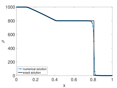
(a) mixture density

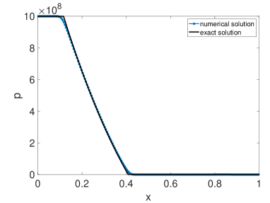
(b) pressure

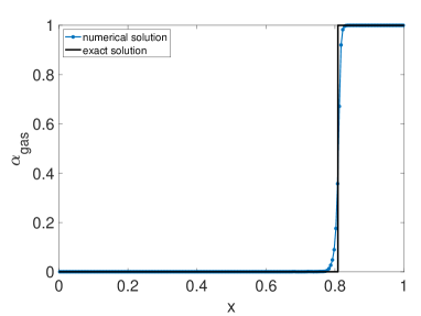
(c) gas volume fraction

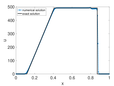
(d) velocity

Figure 1: Numerical solutions (dots), in comparison to exact ones (black lines), of the water-air shock tube problem. The mixture density, pressure, gas volume fraction, and velocity are displayed in subfigures.

Example 3. Two-phase water-air problem. This is the case considered in [36]. Let the mixture of water and air occupy the interval $[0,1]$. The EOSs of water and air are the same as those used in the previous case. The mixture remains at rest initially. The initial condition is given as follows:

$$(\alpha_{1},\ \rho_{1},\ \rho_{2},\ p)=\left\{\begin{array}[]{lr}(0.5,\ 1000,\ 50,\ 10^{9}),&x<0.5,\\[5.69054pt] (0.5,\ 1000,\ 50,\ 10^{5}),&x>0.5.\end{array}\right.$$

Perform the simulation with $200$ equally distributed grids to the time $T=2\times 10^{-4}$. The numerical results obtained by the propose finite volume scheme are displayed in Fig. 2, and an excellent agreement with exact solutions is observed. In addition, the numerical results match well with those obtained by the seven-equation model presented in [36].

(a) mixture density

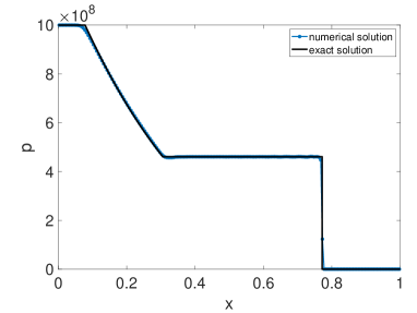
(b) pressure

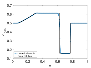
(c) gas volume fraction

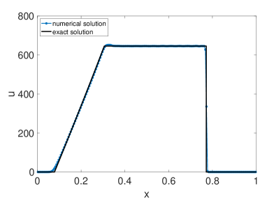
(d) velocity

Figure 2: Numerical solutions (dots), in comparison to exact ones (black lines), of the two-phase water-air problem. The mixture density, pressure, gas volume fraction, and velocity are displayed in subfigures.

Example 4. Cavitation test. This is the case considered in [48]. Once again, the mixture of water and air occupies the interval $[0,1]$ and the EOSs of water and air are the same as those used in Example 2. The initial condition is given as follows,

$$(\alpha_{1},\ \rho_{1},\ \rho_{2},\ u,\ p)=\left\{\begin{array}[]{lr}(0.99,\ 1000,\ 1,\ -100,\ 10^{5}),&x<0.5,\\[5.69054pt] (0.99,\ 1000,\ 1,\ \ \ 100,\ 10^{5}),&x>0.5.\end{array}\right.$$

This case demonstrates the ability of the Kapila model to create an interface which does not exist initially. Perform the numerical computation with $500$ cells to the time $T=1.85$. The numerical results are displayed in Fig. 3 in comparison with exact ones, where a good agreement is observed.

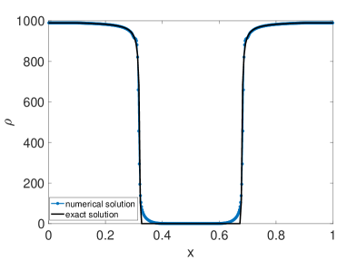
(a) mixture density

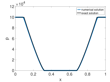
(b) pressure

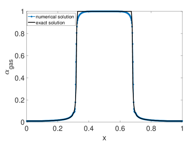
(c) gas volume fraction

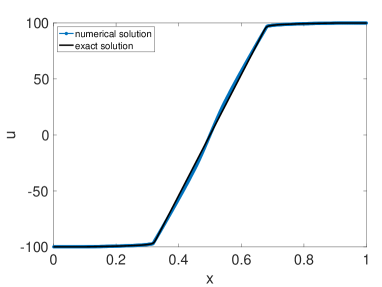
(d) velocity

Figure 3: Numerical solutions (dots), in comparison to exact ones (black lines), of the cavitation test. The mixture density, pressure, gas volume fraction, and velocity are displayed in subfigures.

Example 5. Interaction of a shock in air with a cylindrical helium bubble. This is a 2D test case [50, 40] with experimental data in [16]. The computational domain is divided into regions shown in Fig. 4, with $a=89$ cm, $b=329.3$ cm, $c=50$ cm, $d=25$ cm, and $e=100$ cm. The dashed line indicates the initial position of the left-moving shock. The cylindrical bubble is filled with helium while the rest part of the computational domain is filled with air. Both air and helium are considered as ideal gases with $\gamma_{1}=1.4$ for air and $\gamma_{2}=1.648$ for helium. The pre-shock air and the bubble remain at rest initially and the pre-shock pressure is $1$ atm. The initial density of the bubble is $0.1819~{}\text{kg}/\text{m}^{3}$ and the initial density of the pre-shock air is $1~{}\text{kg}/\text{m}^{3}$. The post-shock state is determined by the shock Mach number $\text{Ma}=1.22$.

Figure 4: The computational domain of the shock-bubble interaction. The dashed line indicates the initial position of the left-moving shock.

The numerical computation is performed using $740\times 100$ cells, in the upper half of the computational domain due to the symmetry of the flow field. Pseudo-color plots of the mixture density and the air volume fraction are shown in Fig 5 at $62\mu s$, $245\mu s$, $427\mu s$, and $983\mu s$ after the shock impacts the cylinder. A good agreement with the experimental results is observed [16, Fig. 7].

(a) $62\mu s$

(b) $245\mu s$

(c) $427\mu s$

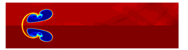
(d) $983\mu s$

Figure 5: Interaction of a shock in air with a helium cylinder. The mixture density (upper half of each figure) and the air volume fraction (lower half of each figure) are shown at $62\mu s$, $245\mu s$, $427\mu s$, and $983\mu s$ after the shock impact the cylinder.

Example 6. Interaction of a shock in water with a cylindrical air bubble. This is another widely considered two-dimensional case [50, 54]. Here we use the set-up in [54]. The computational domain is divided into regions demonstrated in Fig. 4, with $a=12$, $b=12$, $c=6$, $d=2.4$, and $e=0.6$. The cylindrical bubble is filled with air while the rest part of the computational domain is filled with water. The pre-shock water and the bubble remain at rest initially and the pre-shock pressure is $1$. The initial density of the pre-shock water is $1$ and that of the bubble is $0.0012$. The post-shock state is determined by the shock Mach number $\text{Ma}=1.72$. Both water and air follow the stiffened gas EOS (7). The parameters for water are taken to be $\gamma_{1}=4.4$ and $\pi_{1}=6000$, while those for air are taken to be $\gamma_{2}=1.4$ and $\pi_{2}=0$.

By considering the symmetry of the flow field, we perform the numerical computation in the upper half of the computational domain with $240\times 120$ cells. Pseudo-color plots of the mixture density and the water volume fraction are displayed in Fig 6 at computational times $t=0.015$, $t=0.020$, $t=0.025$, $t=0.030$, $t=0.035$, and $t=0.040$, respectively. A good agreement with the numerical results in [54] is observed.

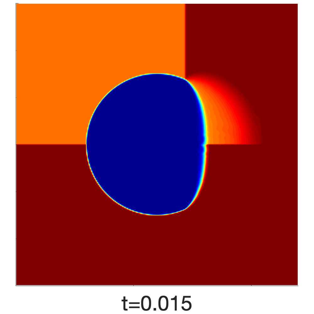
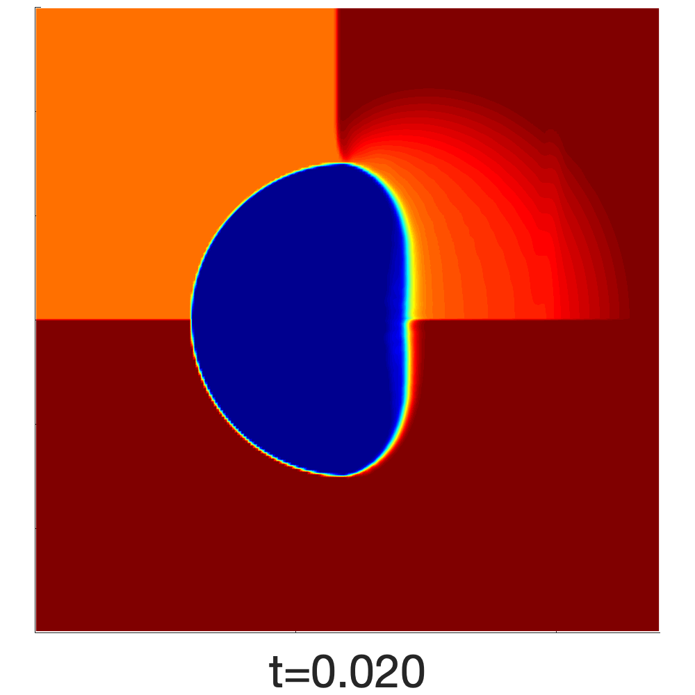
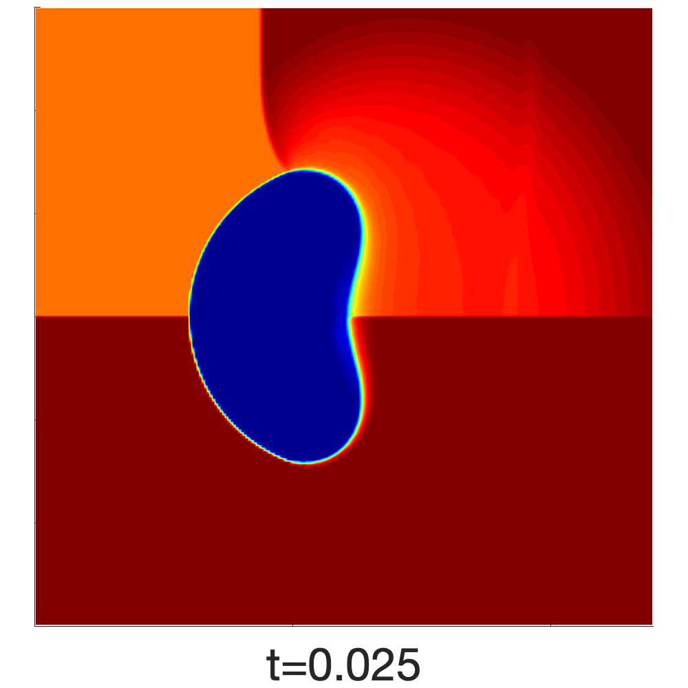
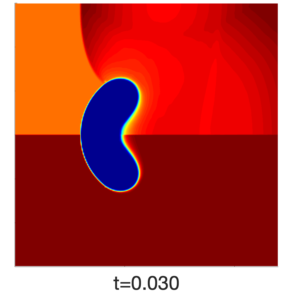
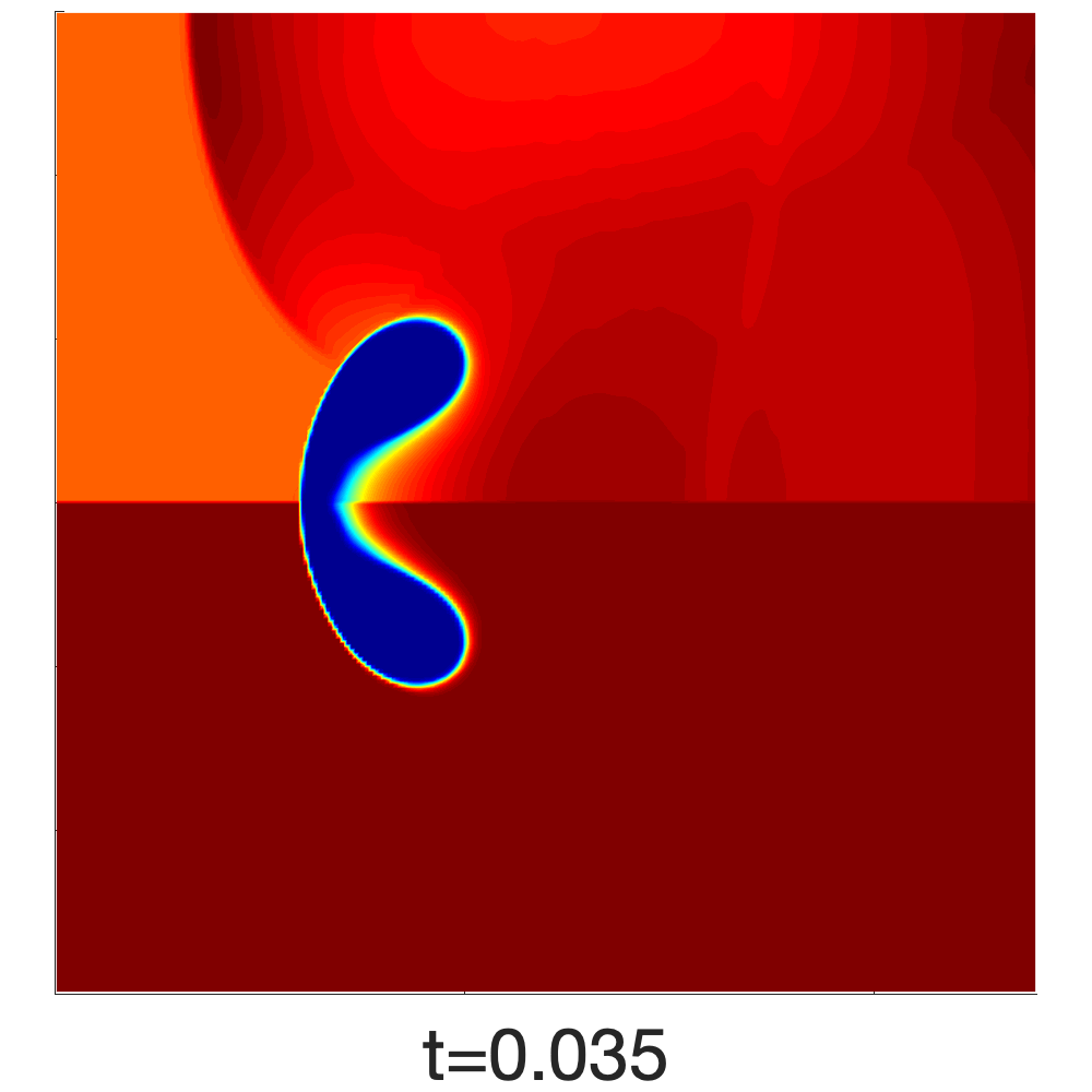
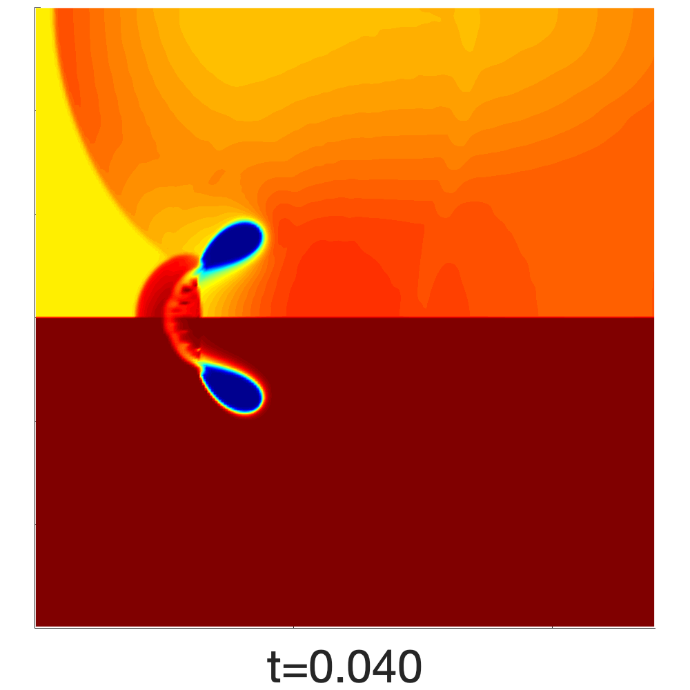
Figure 6: Interaction of a shock in water with a cylindrical air bubble. The mixture density (upper half of each figure) and the water volume fraction (lower half of each figure) are shown at computational times $t=0.015$, $t=0.020$, $t=0.025$, $t=0.030$, $t=0.035$, and $t=0.040$, respectively.

5 Conclusions

The Kapila model, derived from the seven-equation model by asymptotic analysis, is widely used in numerical simulations of compressible multiphase flows involving both fluid mixtures and pure fluids [34, 36, 24, 51, 43, 37]. By adopting the GRP solver, the present paper contributes to the development of a second-order accurate finite volume scheme for the Kapila model, within the temporal-spatial coupling framework. Given the challenges posed by the stiffness of the Kapila model, the proposed scheme enhances the robustness through two key improvements, a semi-implicit time discretization to the stiff source term and the use of temporal-spatial coupling numerical fluxes. The performance of the numerical scheme is demonstrated by several challenging test cases involving either interfaces exhibiting large pressure and density ratios or multiphase fluid mixtures. A nonlinear multiphase flow test case with a smooth solution is proposed to verify the numerical accuracy.

Following the methodology proposed in this paper, it is highlighted that the nonlinear GRP solver becomes essential for simulations of multiphase flows involving strong nonlinear waves. This is demonstrated through the shock tube problem of Example 2 in Section 4, which involves the interface exhibiting dramatic pressure and density ratios. The detailed development of the nonlinear GRP solver for the Kapila model will be presented in our forthcoming paper [12], where detailed insights will be provided.

Appendix A Space data reconstruction

To complete the finite volume scheme, the linear data reconstruction proposed in [6, 7] is adopted. Here we apply the linear reconstruction to primitive variables $\mathbf{W}=[\zeta_{1},\rho,u,v,p,\alpha_{1}]^{\top}$.

In two space dimensions, $\mathbf{W}$ is linearly reconstructed in cell $\Omega_{ij}$ as

$$\mathbf{W}^{n+1}_{i,j}(\mathbf{x})=\widetilde{\mathbf{W}}_{i,j}^{n+1}+(\nabla\mathbf{W})_{i,j}^{n+1}\cdot(\mathbf{x}-\mathbf{x}_{i,j}).$$ (45)

The cell centered value $\widetilde{\mathbf{W}}_{i,j}^{n+1}$ is computed using cell average values $\overline{\mathbf{U}}_{i,j}^{n+1}$ obtained in (13). The approximation to the slope is

$$\left(\displaystyle{\frac{\partial\mathbf{W}}{\partial x}}\right)_{i,j}^{n+1}=\mbox{minmod}\left(\displaystyle{\frac{\widetilde{\mathbf{W}}_{i,j}^{n+1}-\widetilde{\mathbf{W}}_{i-1,j}^{n+1}}{\Delta x}},\kappa\displaystyle{\frac{\widehat{\mathbf{W}}_{i+\frac{1}{2},j}^{n+1}-\widehat{\mathbf{W}}_{i-\frac{1}{2},j}^{n+1}}{\Delta x}},\displaystyle{\frac{\widetilde{\mathbf{W}}_{i+1,j}^{n+1}-\widetilde{\mathbf{W}}_{i,j}^{n+1}}{\Delta x}}\right),$$ (46)

where the cell interface values are computed as

$$\widehat{\mathbf{W}}_{i+\frac{1}{2},j}^{n+1}=\displaystyle\sum_{g}\omega_{g}\widehat{\mathbf{W}}_{i+\frac{1}{2},j}^{n+1,g},\ \ \widehat{\mathbf{W}}_{i+\frac{1}{2},j}^{n+1}=\mathbf{W}_{i+\frac{1}{2},j}^{n,*,g}+\left(\displaystyle{\frac{\partial\mathbf{W}}{\partial t}}\right)_{i+\frac{1}{2},j}^{n,*,g}.$$ (47)

The coefficient $\kappa\in[0,2)$ is a user-tuned parameter. The minmod function is defined as

$$\mbox{minmod}(a,b,c)=\left\{\begin{array}[]{ll}\text{sign}(a)\min(|a|,|b|,|c|),&\text{if }\text{sign}(a)=\text{sign}(b)=\text{sign}(c),\\ 0,&\text{otherwise}.\end{array}\right.$$ (48)

The other component $(\partial\mathbf{W}/\partial y)_{i,j}^{n+1}$ of the gradient can be computed similarly. By transforming the reconstructed piecewise linear function of $\mathbf{W}$ into those of $\mathbf{U}$, the initial value to be used in the IVP (33) is obtained.

References

- [1] B. Albertazzi, P. Mabey, T. Michel, G. Rigon, J. R. Marquès, S. Pikuz, S. Ryazantsev, E. Falize, L. V. B. Som, J. Meinecke, N. Ozaki, G. Gregori, and M. Koenig, Triggering star formation: Experimental compression of a foam ball induced by Taylor–Sedov blast waves, Matter Radiat. Extremes, 7 (2022), p. 036902.
- [2] N. Andrianov, R. Saurel, and G. Warnecke, A simple method for compressible multiphase mixtures and interfaces, Int. J. Numer. Methods Fluids, 41 (2003), pp. 109–131.
- [3] N. Andrianov and G. Warnecke, The Riemann problem for the Baer-Nunziato two-phase flow model, J. Comput, Phys., 212 (2004), pp. 434–464.
- [4] M. R. Baer and J. W. Nunziato, Two-phase modeling of deflagration-to-detonation transition in granular materials: A critical examination of modeling issues, Int. J. Multiphase Flow, 12 (1986), pp. 861–889.
- [5] M. Ben-Artzi and J. Falcovitz, A second-order Godunov-type scheme for compressible fluid dynamics, J. Comput. Phys., 55 (1984), pp. 1–32.
- [6] M. Ben-Artzi and J. Falcovitz, Generalized Riemann Problems in Computational Fluid Dynamics, Cambridge University Press, Cambridge, 2003.
- [7] M. Ben-Artzi, J. Li, and G. Warnecke, Direct Eulerian GRP scheme for compressible fluid flows, J. Comput, Phys., 31 (2006), pp. 335–362.
- [8] R. Caiden, R. P. Fedkiw, and C. Anderson, A numerical method for two-phase flow consisting of separate compressible and incompressible regions, J. Comput. Phys., 166 (2001), pp. 1–27.
- [9] A. Chinnayya, E. Daniel, and R. Saurel, Modelling detonation waves in heterogeneous energetic materials, J. Comput. Phys., 196 (2004), pp. 769–774.
- [10] Y. Y. Chu, Z. Wang, J. M. Qi, Z. P. Xu, and Z. H. Li, Numerical performance assessment of double-shell targets for z-pinch dynamic hohlraum, Matter Radiat. Extremes, 7 (2022), p. 035902.
- [11] V. Deledicque and M. V. Papalexandris, An exact Riemann solver for compressible two-phase flow models containing non-conservative products, J. Comput. Phys., 222 (2007), pp. 217–245.
- [12] Z. Du, Generalized Riemann problem method for the Kapila model of compressible multiphase flows II: Nonlinear flux solver. Paper in preparation, 2023.
- [13] Z. Du and J. Li, A Hermite WENO reconstruction for fourth order temporal accurate schemes based on the GRP solver for hyperbolic conservation laws, J. Comput, Phys., 355 (2018), pp. 3045–3069.
- [14] M. Dumbser, D. S. Balsara, E. F. Toro, and C.-D. Munz, A unified framework for the construction of one-step finite volume and discontinuous Galerkin schemes on unstructured meshes, J. Comput. Phys., 227 (2008), pp. 8209–8253.
- [15] R. F. F. Gibou and S. Osher, A review of level-set methods and some recent applications, J. Comput. Phys., 353 (2018), pp. 82–109.
- [16] J.-F. Haas and B. Sturtevant, Interaction of weak shock waves with cylindrical and spherical gas inhomogeneities, J. Fluid Mech., 181 (1987), pp. 41–76.
- [17] Y. Hu, Q. Shi, V. F. De Almeida, and X. Li, Numerical simulation of phase transition problems with explicit interface tracking, Chem. Eng. Sci., 128 (2015), pp. 92–108.
- [18] X. Ji, L. Pan, W. Shyy, and K. Xu, A compact fourth-order gas-kinetic scheme for the Euler and Navier-Stokes equations, J. Comput, Phys., 372 (2018), pp. 446–472.
- [19] X. Ji, F. Zhao, W. Shyy, and K. Xu, A HWENO reconstruction based high-order compact gas-kinetic scheme on unstructured mesh, J. Comput, Phys., 410 (2020), p. 109367.
- [20] H. Kamaya, On the origin of small-scale structure in self-gravitating two-phase gas, Astrophys. J., 465 (1996), pp. 769–774.
- [21] A. K. Kapila, R. Menikoff, J. B. Bdzil, and S. F. Son, Two-phase modeling of deflagration-to-detonation transition in granular materials: Reduced equations, Phys. Fluids, 13 (2001), pp. 3002–3024.
- [22] A. K. Kapila, S. F. Son, J. B. Bdzil, R. Menikoff, and D. S. Stewart, Two-phase modeling of DDT: Structure of the velocity-relaxation zone, Phys. Fluids, 9 (1997), pp. 3885–3897.
- [23] S. Karni and G. Hernández-Dueñas, A hybrid algorithm for the Baer-Nunziato model using the Riemann invariants, J. Sci. Comput., 45 (2010), pp. 382–403.
- [24] J. J. Kreeft and B. Koren, A new formulation of Kapila’s five-equation model for compressible two-fluid flow, and its numerical treatment, J. Comput, Phys., 229 (2010), pp. 6220–6242.
- [25] K. Lan, Dream fusion in octahedral spherical hohlraum, Matter Radiat. Extremes, 7 (2022), p. 055701.
- [26] P. D. Lax and B. Wendroff, Systems of conservation laws, Comm. Pure Appl. Math., 13 (1960), pp. 217–237.
- [27] O. Le Metayer, J. Massoni, and R. Saurel, Modelling evaporation fronts with reactive Riemann solvers, J. Comput. Phys., 205 (2005), pp. 567–610.
- [28] X. Lei and J. Li, Transversal effects and genuine multidimensionality of high order numerical schemes for compressible fluid flows, Appl. Math. Mech. -Engl. Ed., 39 (2018), pp. 1–12.
- [29] X. Lei and J. Li, A staggered-projection Godunov-type method for the Baer-Nunziato two-phase model, J. Comput. Phys., 437 (2021), p. 110312.
- [30] J. Li, Two-stage fourth order: temporal-spatial coupling in computational fluid dynamics (CFD), Adv. Aerodyn, 1 (2019), pp. 1–36.
- [31] J. Li and Y. Wang, Thermodynamical effects and high resolution methods for compressible fluid flows, J. Comput. Phys., 343 (2017), pp. 340–354.
- [32] M. A. Liberman, Combustion Physics: Flames, Detonations, Explosions, Astrophysical Combustion and Inertial Confinement Fusion, Springer Nature, Switzerland, 2021.
- [33] I. S. Men’shov, The generalized problemm of breakup of an arbitrary discontinuity, J. Appl. Maths Mechs., 55 (1991), pp. 67–74.
- [34] G. H. Miller and E. G. Puckett, A high-order Godunov method for multiple condensed phases, J. Comput, Phys., 128 (1996), pp. 134–164.
- [35] G. I. Montecinos, A. Santacá, M. Celant, L. O. Müller, and E. F. Toro, A unified framework for the construction of one-step finite volume and discontinuous Galerkin schemes on unstructured meshes, Comput. & Fluids, 248 (2022), p. 105685.
- [36] A. Murrone and H. Guillard, A five equation reduced model for compressible two phase flow problems, J. Comput, Phys., 202 (2005), pp. 664–698.
- [37] F. Petitpas, E. Franquet, R. Saurel, and O. Le Metayer, A relaxation-projection method for compressible flows. Part II: Artificial heat exchanges for multiphase shocks, J. Comput. Phys., 225 (2007), pp. 2214–2248.
- [38] F. Petitpas, J. Massoni, R. Saurel, E. Lapebie, and L. Munier, Diffuse interface model for high speed cavitating underwater systems, Int. J. Multiphase Flows, 35 (2009), pp. 747–759.
- [39] F. Petitpas, R. Saurel, E. Franquet, and A. Chinnayya, Modelling detonation waves in condensed materials: multiphase cj conditions and multidimensional computations, Shock Waves, 19 (2009), pp. 377–401.
- [40] J. J. Quirk and S. Karni, On the dynamics of a shock-bubble interaction, J . Fluid Mech., 318 (1996), pp. 129–163.
- [41] V. Rana, H. Lim, J. Melvin, J. Glimm, B. Cheng, and D. H. Sharp, Mixing with applications to inertial-confinement-fusion implosions, Phys. Rev. E, 95 (2017), p. 013203.
- [42] R. Saurel and R. Abgrall, A multiphase Godunov method for compressible multifluid and multiphase flows, J. Comput, Phys., 150 (1999), pp. 425–467.
- [43] R. Saurel, E. Franquet, E. Daniel, and O. Le Metayer, A relaxation-projection method for compressible flows. Part I: The numerical equation of state for Euler equations, J. Comput. Phys., 223 (2007), pp. 822–845.
- [44] R. Saurel and O. Le Metayer, A multiphase model for interfaces, shocks, detonation waves and cavitation, J. Comput. Phys., 431 (2001), pp. 239–271.
- [45] R. Saurel, O. Le Metayer, J. Massoni, and S. Gavrilyuk, Shock jump relations for multiphase mixtures with stiff mechanical relaxation, Shock Waves, 16 (2007), pp. 209–232.
- [46] R. Saurel and C. Pantano, Diffuse-interface capturing methods for compressible two-phase flows, Annu. Rev. Fluid Mech., 50 (2018), pp. 105–130.
- [47] R. Saurel, F. Petitpas, and R. Abgrall, Modelling phase transition in metastable liquids: application to cavitating and flashing flows, J. Fluid Mech., 607 (2008), pp. 313–350.
- [48] R. Saurel, F. Petitpas, and R. A. Berry, Simple and efficient relaxation methods for interfaces separating compressible fluids, cavitating flows and shocks in multiphase mixtures, J. Comput, Phys., 228 (2009), pp. 1678–1712.
- [49] D. W. Schwendeman, C. W. Wahle, and A. K. Kapila, The Riemann problem and a high-resolution Godunov method for a model of compressible two-phase flow, J. Comput. Phys., 212 (2006), pp. 490–526.
- [50] H. Terashima and G. Tryggvason, A front-tracking/ghost-fluid method for fluid interfaces in compressible flows, J. Coumpt. Phys., 228 (2009), pp. 4012–4037.
- [51] B. Tian and L. Li, A five-equation model based global ALE method for compressible multifluid and multiphase flows, Comput. & Fluids, 241 (2021), pp. 149–172.
- [52] E. F. Toro and V. A. Titarev, Derivative Riemann solvers for systems of conservation laws and ADER methods, J. Comput. Phys., 212 (2006), pp. 150–165.
- [53] A. Wood, A Textbook of Sound, MacMillan, New York, 1930.
- [54] L. Xu and T. Liu, Explicit interface treatments for compressible gas-liquid simulations, Comput. & Fluids, 153 (2017), pp. 34–48.