Fast word error rate estimation using self-supervised representations for speech and text

Abstract

The quality of automatic speech recognition (ASR) is typically measured by word error rate (WER). WER estimation is a task aiming to predict the WER of an ASR system, given a speech utterance and a transcription. This task has gained increasing attention while advanced ASR systems are trained on large amounts of data. In this case, WER estimation becomes necessary in many scenarios, for example, selecting training data with unknown transcription quality or estimating the testing performance of an ASR system without ground truth transcriptions. Facing large amounts of data, the computation efficiency of a WER estimator becomes essential in practical applications. However, previous works usually did not consider it as a priority. In this paper, a Fast WER estimator (Fe-WER) using self-supervised learning representation (SSLR) is introduced. The estimator is built upon SSLR aggregated by average pooling. The results show that Fe-WER outperformed the e-WER3 baseline relatively by 19.69% and 7.16% on Ted-Lium3 in both evaluation metrics of root mean square error and Pearson correlation coefficient, respectively. Moreover, the estimation weighted by duration was 10.43% when the target was 10.88%. Lastly, the inference speed was about 4x in terms of a real-time factor.

Index Terms—  Word error rate, WER estimator, self-supervised representation, inference speed, multiple layer perceptrons

1 Introduction

Word error rate (WER) is a commonly used metric for evaluating ASR systems. It is the ratio between the number of substitution, insertion and deletion errors in a hypothesis and the number of words in a reference. In some scenarios, it can be very useful to use a model to estimate the WER of an ASR system. For example, a WER estimator can be used to select unlabelled data for ASR self-training [1, 2, 3]. Another use may be to filter out training data with low-quality transcriptions, especially for recent ASR models (e.g. Whisper [4]) that are trained with large amounts of data collected from the Internet. The transcriptions of data collected from the Internet are often of low quality. In order to achieve good ASR performance, data samples with low-quality transcriptions usually need to be excluded for ASR training. A common method for data filtering is to quickly estimate a WER for each sample in the collected dataset and then remove samples with a WER higher than a threshold. Dealing with large amounts of data collected from the Internet, the computational efficiency of a WER estimator becomes important. Lastly, in order to estimate the WER of ASR systems, one obvious solution is to produce confidence scores from the ASR system itself [5, 6]. This method does not require building another model. However, this has the risk of bias - and as will be shown - does not perform well in comparison to other methods.

The prediction of ASR errors and WER were researched in [7] using a stacked auto-encoder. The authors suggested detecting erroneous words and estimating WER from the number of errors. Recently, researchers proposed to directly estimate the WER of ASR systems without the need for decoding. These works include e-WER [8], e-WER2 [9] and e-WER3 [10]. e-WER3 used bidirectional long short-term memory (BiLSTM) networks to extract features for speech, while the text features were averaged over tokens. Then, WER was estimated using those features without ASR decoding. Additionally, WER estimation has been also studied in [11] as a part of speech intelligibility.

Although e-WER based models have obtained impressive progress on estimating the WER of ASR systems, there are still several questions not being fully studied. Although the e-WER3 model avoided ASR decoding, it is still built upon BiLSTMs. While the architecture with recurrent neural networks (RNNs) is capable of capturing the sequential information, it is computationally expensive to deal with long sequences, such as a spoken utterance. This could limit the use of long speech for training. Secondly, the performance of the estimator would depend on the input features for speech and text. Thus, the different combination of SSLRs for speech and text needs to be explored for optimal performance on the WER estimation task. Lastly, the performance needs to be analysed across data attributes, such as utterance lengths and speakers in addition to the evaluation metrics. In this paper, a framework to build a Fast WER estimator (Fe-WER) consisting of speech and text encoders, feature aggregators and a WER estimator, is proposed. The SSLRs aggregated by average pooling are used to directly estimate WER with multiple layer perceptrons (MLP). This framework will be explored from an accuracy and efficiency perspective.

The contributions of this paper are as following:

1. This paper proposes a new WER estimator, Fe-WER, which outperforms the baseline model, e-WER3, on computation efficiency without performance degradation. While the performance improved by relative 19.69% and 7.16% in root mean square error (RMSE) and Pearson correlation coefficient (PCC), the inference time is reduced by 78.09% in real-time factor (RTF). The weighted WER estimation by duration is 10.43%, when the target is 10.88%.

2. The experimental evidence shows that the combination of HuBERT [12] and XLM-R [13] for speech and text, respectively, obtained the best performance on WER estimation.

3. The RMSE on short utterances decreases when long utterances are not added to the training dataset.

2 Related works

2.1 WER estimation

There have been few works on WER estimation. First, e-WER3 is a WER estimator recently proposed for multiple languages. In [10], hypotheses were generated by a conformer-based ASR system [14] trained on LibriSpeech [15]. The features of utterances and hypotheses were extracted using XLSR-53 [16] and XLM-R [13]. The hidden states of BiLSTM on both directions over frame-level representations were concatenated as an utterance-level representation, while a transcript-level representation was averaged over token-level representations. For data selection, the hypotheses with a WER equal to 0 were selected up to the number of hypotheses in the second and third highest frequency bins. The WER was predicted using fully connected layers. The result was 0.14 and 0.66 in RMSE and PCC on the English corpus, Ted-Lium3 [17], which was improved by 9% in PCC from e-WER2.

In the recent literature [11], a WER prediction system was used as one of the multiple tasks for speech intelligibility prediction. Three types of acoustic representations were generated by the short-time Fourier transform, learnable filter banks and HuBERT. The concatenated representation was used as an input to BiLSTM followed by a fully connected layer to extract features. Next, the HuBERT model and the estimator were jointly trained to predict WER of output of Google Cloud Speech-to-Text. The performance on WER estimation was 0.1760 and 0.822 in RMSE and Spearman’s rank correlation coefficient on the Taiwan Mandarin corpus [18].

3 Fast word error rate estimation

3.1 Architecture

In this work we propose Fe-WER (see Fig. 1), which is based on a two-tower architecture [19, 20]. It maps different representations into a shared space to capture the similarity between two inputs. The proposed model consists of two aggregators for speech and text and fully connected layers which performs the WER estimation. The aggregators convert the features extracted by SSLRs into a sequence-level representation. After that, two sequence-level representations are concatenated as an input to multi-layer perceptrons (MLP) consisting of fully connected layers with a rectified linear unit (ReLU). A sigmoid function is applied to the output.

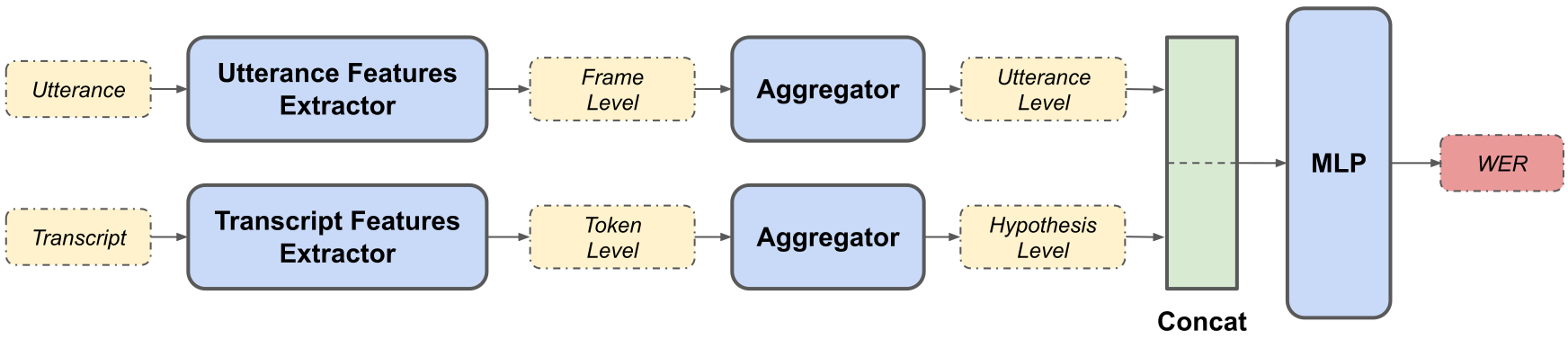
Fig. 1: Illustration of the proposed method for WER estimation

3.2 Training objective

The mean squared error (MSE) between $WER$ and $\widehat{WER}$ is used as the objective function, where $WER$ is between references and hypotheses and $\widehat{WER}$ is the estimation by the model.

$$MSE=\frac{\sum_{i=1}^{N}(WER_{i}-\widehat{WER}_{i})^{2}}{N}$$ (1)

where $N$ is the number of instances in a dataset and $i$ is an index of an instance.

3.3 Evaluation metrics

PCC and RMSE are used as an evaluation metric. PCC indicates that two variables change in the same direction if the coefficient is close to 1, while in the opposite direction if it is close to -1.

$$\rho=\frac{\sum_{i=1}^{N}(WER_{i}-\mu_{WER})(\widehat{WER}_{i}-\mu_{\widehat{WER}})}{\sqrt{\sum_{i=1}^{N}(WER_{i}-\mu_{WER})^{2}\sum_{i=1}^{N}(\widehat{WER}_{i}-\mu_{\widehat{WER}})^{2}}}$$ (2)

where $\mu_{WER}$ is the mean of $WER$. Moreover, the word error estimate weighted by duration is measured as defined below:

$$\widehat{WER}_{dur}=\frac{\sum_{i=1}^{N}(\widehat{WER}_{i}\times Duration_{i})}{\sum_{p=1}^{N}(Duration_{i})}$$ (3)

where $i$ is an index of a pair of an utterance and a hypothesis. Similarly, the word error estimate can be weighted by the number of words in a reference transcript, $\widehat{WER}_{wrd}$. Lastly, the ratio between weighted $WER_{wrd}$ and $\widehat{WER}_{dur}$ is also measured. The WER estimation is weighted by duration because the reference is not known when it is estimated.

$$WERR=\frac{|WER_{wrd}-\widehat{WER}_{dur}|}{WER_{wrd}}.$$ (4)

4 Experimental setup

4.1 Baseline WER estimators

The proposed model was compared with two baselines: Whisper large[4] and e-WER3. First, an intuitive way to estimate the correctness of a hypothesis by using the ASR system is to use the ASR system itself. The average log probability over the output tokens can be an estimate for the errors in the hypothesis. Thus, the value subtracted from 1 was used as a WER estimate on the hypothesis. Second, e-WER3 was used as another baseline as described in [10]. Although the model was proposed for multiple languages, it outperformed its previous model, e-WER2, on an English corpus.

4.2 Data

TED-LIUM3 (TL3) [17] is a corpus of TED talks and is summarised in Table 1. It was used for evaluating Whisper on speech recognition and e-WER3 on WER estimation. For WER estimation, TL3 was transcribed using the Whisper large model to get target WER. Whisper’s text normaliser was modified not to replace numeric expressions with a form using Arabic numbers.

Table 1: Statistics of TL3 datasets

Dataset	# of seg.	total dur.	avg. dur.	avg. #wrd.
eval	2710	4.61h	6.12s	18.16
dev	2582	4.59h	6.40s	17.13
train	262971	444.62h	6.09s	17.42

In order to deal with imbalanced data, data were selected as described in the e-WER3 paper [10]. For example, utterances shorter up to a length of 10 seconds were selected and WER was reduced to range 0% to 100%. These datasets with duration limit are noted with (D), e.g. TL3 train (D), while the datasets selected without the duration limit are noted with (A), meaning all duration. The statistics of the data selected are described in Table 2.

Table 2: Statistics of the sets of data selected. Hypotheses were generated by Whisper large on TL3 datasets.

Dataset	#seg.	total dur. (h)	avg. WER	std. dev.	weighted WER
eval (D)	842	1.41	0.1429	0.1997	0.1088
dev (D)	1034	1.70	0.1532	0.2247	0.1225
train (D)	123255	200.55	0.2434	0.3209	0.2029
eval (A)	1023	1.98	0.1307	0.1935	0.0979
dev (A)	1190	2.18	0.1411	0.2174	0.1091
train (A)	140852	256.22	0.2334	0.3184	0.1913

4.3 Self-supervised learning representations

SSLRs of similar sizes were selected considering their performance on benchmarks for speech and language [21, 22, 23]. SSLRs were the pre-trained large models of HuBERT [12], data2vec for audio [24] and WavLM [25] for speech as well as RoBERTa [26], DeBERTaV3 large [27] and GPT-2 medium [28] models for text. Moreover, two models adopted by the e-WER3 baseline were also added: fine-tuned XLSR-53 large and XLM-RoBERTa large.

4.4 Fe-WER

Average pooling over the frame or the token dimension was adopted as an aggregator. The WER estimator consists of multi-layer perceptrons of 2 hidden layers and 1 output layer followed by activation functions on top of the concatenated feature layer. Moreover, the output of each layer is normalised as well as dropout is applied to the hidden layers.

Hyper-parameters for Fe-WER were chosen by grid search. The optimizer was Adam with a learning rate of 1e-3. In addition to the fixed dropout of 0.1, ReLU and Sigmoid were chosen as the activation functions for hidden and output layers, respectively. The fully-connected layers were 3 layers of 600, 32 and 1 nodes on top of the input features of 2048 dimensions. With the parameters, the WER estimator was trained using a cosine annealing scheduler and an early stop of 40 epochs.

4.5 Evaluation

RMSE, PCC and WERR in Section 3.3 were measured on test datasets as evaluation metrics. The WERR is obtained by calculating the target WER weighted by the number of words in reference and the WER estimation weighted by duration. In the case of WER estimation when the reference is not known, duration can be used instead of the exact number of words in the reference.

5 Results

5.1 Comparison with baselines

WER on TL3 dev and eval (D) was estimated by the two baseline systems introduced in Section 4.1. First, Table 3 shows that the PCC values of both baselines are over 0.5, which is known to have correlation between the variables. Second, the RMSE of Whisper was surpassed by e-WER3 and even higher than the standard deviation of the target WER on TL3 dev and eval (D) in Table 2. Next, two aggregation strategies were compared to each other using XLSR and XLM-R: BiLSTM (e-WER3) and average pooling (Fe-WER) in Table 3. The first strategy was to use the concatenation of the final hidden states of BiLSTM on both directions as an utterance-level representation, while the second used the representation averaged over frames. The average pooling for a spoken utterance outperformed the other on the TL3 dev and eval (D) in both RMSE and PCC. Moreover, the performance of Fe-WER was improved when HuBERT and XLM-R were used as SSLRs for utterances and hypotheses instead of XLSR and XLM-R. When the best performance of Fe-WER is compared with the e-WER3 baseline, RMSE and PCC of Fe-WER on TL3 eval (D) were relatively improved by 19.69% and 7.16%, respectively, from those of the e-WER3 baseline.

Table 3: Performance of baseline systems and Fe-WER with different combinations of SSLRs on TL3 val (D). XS: XLSR, HU: HuBERT, DA: Data2vec, WA: WavLM, XM: XLM-R, RO: RoBERTa, DE: DeBERTaV3, GP: GPT-2.

model	SSLR		dev		eval
	Utt.	Hyp.	RMSE$\downarrow$	PCC$\uparrow$	RMSE$\downarrow$	PCC$\uparrow$
Whisper	-		0.2579	0.7015	0.2555	0.6739
e-WER3	XS	XM	0.1126	0.8644	0.1082	0.8419
Fe-WER	XS	XM	0.1103	0.8720	0.1008	0.8662
	XS	RO	0.1142	0.8614	0.1035	0.8579
	XS	DE	0.1121	0.8666	0.1133	0.8296
	XS	GP	0.1110	0.8699	0.1089	0.8428
	HU	XM	0.1008	0.8928	0.0869	0.9022
	HU	RO	0.1164	0.8550	0.0955	0.8800
	HU	DE	0.1133	0.8653	0.1025	0.8624
	HU	GP	0.1100	0.8722	0.0982	0.8733
	DA	XM	0.1131	0.8648	0.1016	0.8619
	DA	RO	0.1182	0.8504	0.1095	0.8387
	DA	DE	0.1139	0.8627	0.1105	0.8367
	DA	GP	0.1185	0.8523	0.1084	0.8424
	WA	XM	0.1082	0.8759	0.0954	0.8816
	WA	RO	0.1136	0.8658	0.0984	0.8711
	WA	DE	0.1160	0.8572	0.0984	0.8725
	WA	GP	0.1091	0.8742	0.0948	0.8818

5.2 No duration limit

So far, the models were trained and evaluated on utterances shorter than 10 seconds for comparison with the baselines. When the estimator was trained on the data selected without duration limit, TL3 train (A) in Table 2, the RMSE on the utterances in the range [1,2) and [2,3) seconds increased by 0.0758 and 0.0266 and the PCC decreased by 0.1033 and 0.0878, respectively. The distributions of RMSE and PCC are summarised in Table 4.

Table 4: Distribution of RMSE and PCC on TL3 eval (D).

Duration	RMSE		PCC
(seconds)	train (D)	train (A)	train (D)	train (A)
[1,2)	0.1670	0.2428	0.8998	0.7965
[2,3)	0.1084	0.1350	0.8401	0.7523
[3,4)	0.1252	0.1267	0.8266	0.8229
[4,5)	0.0715	0.0749	0.8685	0.8549
[5,6)	0.0793	0.0885	0.7972	0.7384
[6,7)	0.0736	0.0759	0.8607	0.8517
[7,8)	0.0544	0.0577	0.9082	0.8962
[8,9)	0.0607	0.0647	0.9295	0.9222
[9,10]	0.0651	0.0817	0.8513	0.7522

WERR was also measured to compare the performance of the estimators trained on the two training datasets. The evaluation metrics of weighted WER estimation is defined in Equation (3). While the target WER weighted by words was 0.1088, the WER estimation of the models trained on TL3 train (D) and (A) were 0.1043 and 0.1023, respectively, on TL3 eval (D) when they were weighted by duration. Their WERR were 4.13% and 5.97%, respectively.

5.3 Distributions of target WER and WER estimates

The histograms of the target WER and WER estimates by the estimator on TL3 eval (D) are visualised in Fig. 2. In this figure, the distribution of WER estimates by Fe-WER is similar to that of the target WER. The majority of target WERs are in the range of [0.0, 0.2) as well as that of WER estimates. However, the frequency of target WER of 0 is the highest in the left histogram, while the most frequent estimate is between 0 and 0.1 in the right figure. The reason for this observation is that the estimates tend to be a small number rather than 0 as they are an output of the sigmoid function.

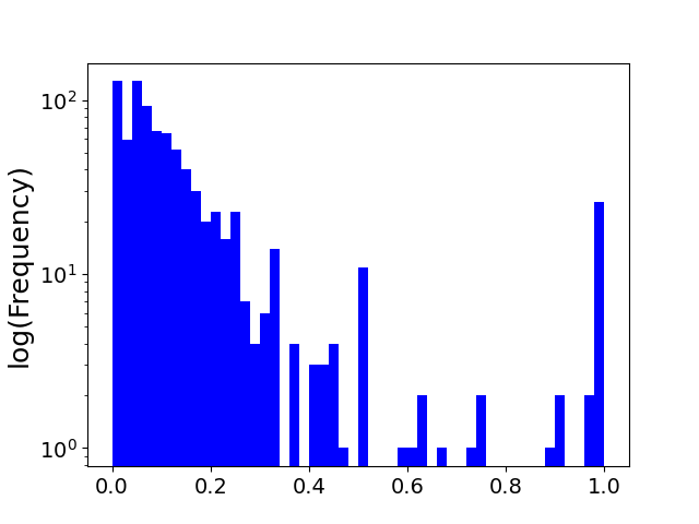
(a) target WER

(b) WER estimated

Fig. 2: Histograms of target WER and estimates on TL3 eval (D)

For further analysis, the average of target WER and WER estimates for each speaker are shown in Fig. 3. The average of WER estimates on each speaker tends to be lower than that of target WER. The higher average of WER estimates than that of target WER is observed on speaker 16 because of the target WER of 0. When the target WER of segments is 0, the average of WER estimates is always higher than 0 as discussed in the previous paragraph. Otherwise, the average of WER estimates tends to be lower than that of target WER.

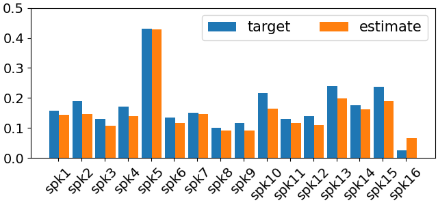
Fig. 3: Average WER per each speaker

5.4 Inference speed

The inference time of the WER estimators was measured excluding the encoding time of utterances and transcripts. The inference time was measured on one GPU of GeForce RTX 3090 with batch size of 1 for comparison purposes. The RTF of e-WER3 was reduced by 78.09% when the WER was estimated by Fe-WER. They are summarised in Table 5.

Table 5: Inference time and real-time factor (RTF) of e-WER3 and Fe-WER on TL3 eval (D) of 5223.01 seconds. RTF stands for real-time factor.

	e-WER3	Fe-WER
total	10.82s	2.37s
RTF	0.002072	0.000454

6 Conclusion

In this paper, a Fast WER estimator has been proposed. This proposed model consists of SSLR encoders for speech and text, aggregators of average pooling and an MLP estimator. The WER estimator outperforms the e-WER3 baseline by relative 19.69% and 7.16% in RMSE and PCC, respectively. In addition, the performance of the estimator could be improved by filtering out long utterances in a training dataset in terms of WERR. Moreover, distributions of target WER and WER estimates were explored over utterance lengths and speakers. Furthermore, the experimental results show the inference speed has been significantly improved, for example, 4x faster than the e-WER3 baseline, without performance degradation.

7 Acknowledgements

This work was conducted at the Voicebase/Liveperson Centre of Speech and Language Technology at the University of Sheffield which is supported by Liveperson, Inc..

References

- [1] Y. Chen, W. Wang, and C. Wang, “Semi-supervised ASR by end-to-end self-training,” in Proc. Interspeech 2020, 2020, pp. 2787–2791.
- [2] J. Kahn, A. Lee, and A. Hannun, “Self-training for end-to-end speech recognition,” in ICASSP 2020 - 2020 IEEE International Conference on Acoustics, Speech and Signal Processing (ICASSP), 2020, pp. 7084–7088.
- [3] Q. Xu, A. Baevski, et al., “Self-training and pre-training are complementary for speech recognition,” in ICASSP 2021 - 2021 IEEE International Conference on Acoustics, Speech and Signal Processing (ICASSP), 2021, pp. 3030–3034.
- [4] A. Radford, J. W. Kim, T. Xu, G. Brockman, C. McLeavey, and I. Sutskever, “Robust speech recognition via large-scale weak supervision,” OpenAI., https://cdn.openai.com/papers/whisper.pdf (Accessed: Jun 22, 2023).
- [5] A. Kumar, S. Singh, D. Gowda, A. Garg, S. Singh, and C. Kim, “Utterance confidence measure for end-to-end speech recognition with applications to distributed speech recognition scenarios,” in Proc. Interspeech 2020, 2020, pp. 4357–4361.
- [6] W. Jeon, M. Jordan, and M. Krishnamoorthy, “On modeling ASR word confidence,” in ICASSP 2020 - 2020 IEEE International Conference on Acoustics, Speech and Signal Processing (ICASSP), 2020, pp. 6324–6328.
- [7] S. Jalalvand and D. Falavigna, “Stacked auto-encoder for asr error detection and word error rate prediction,” in Proc. Interspeech 2015, 2015, pp. 2142–2146.
- [8] A. Ali and S. Renals, “Word error rate estimation for speech recognition: e-WER,” in Proceedings of the 56th Annual Meeting of the Association for Computational Linguistics (Volume 2: Short Papers), Melbourne, Australia, July 2018, pp. 20–24, Association for Computational Linguistics.
- [9] A. Ali and S. Renals, “Word error rate estimation without ASR output: e-WER2,” in Proc. Interspeech 2020, 2020, pp. 616–620.
- [10] S. A. Chowdhury and A. Ali, “Multilingual word error rate estimation: e-WER3,” in ICASSP 2023 - 2023 IEEE International Conference on Acoustics, Speech and Signal Processing (ICASSP), 2023, pp. 1–5.
- [11] R. E. Zezario, S. wei Fu, F. Chen, C.-S. Fuh, H.-M. Wang, and Y. Tsao, “MTI-Net: A multi-target speech intelligibility prediction model,” in Proc. Interspeech 2022, 2022, pp. 5463–5467.
- [12] W.-N. Hsu, B. Bolte, Y.-H. H. Tsai, K. Lakhotia, R. Salakhutdinov, and A. Mohamed, “HuBERT: Self-supervised speech representation learning by masked prediction of hidden units,” IEEE/ACM Transactions on Audio, Speech, and Language Processing, vol. 29, pp. 3451–3460, 2021.
- [13] A. Conneau et al., “Unsupervised cross-lingual representation learning at scale,” in Proceedings of the 58th Annual Meeting of the Association for Computational Linguistics, Online, July 2020, pp. 8440–8451, Association for Computational Linguistics.
- [14] A. Gulati et al., “Conformer: Convolution-augmented Transformer for Speech Recognition,” in Proc. Interspeech 2020, 2020, pp. 5036–5040.
- [15] V. Panayotov, G. Chen, D. Povey, and S. Khudanpur, “Librispeech: An ASR corpus based on public domain audio books,” in 2015 IEEE International Conference on Acoustics, Speech and Signal Processing (ICASSP), 2015, pp. 5206–5210.
- [16] A. Conneau, A. Baevski, R. Collobert, A. Mohamed, and M. Auli, “Unsupervised cross-lingual representation learning for speech recognition,” in Proc. Interspeech 2021, 2021, pp. 2426–2430.
- [17] F. Hernandez, V. Nguyen, S. Ghannay, N. Tomashenko, and Y. Estève, “TED-LIUM 3: Twice as much data and corpus repartition for experiments on speaker adaptation,” in Speech and Computer, A. Karpov, O. Jokisch, and R. Potapova, Eds., Cham, 2018, pp. 198–208, Springer International Publishing.
- [18] Y.-W. Chen and Y. Tsao, “InQSS: A speech intelligibility and quality assessment model using a multi-task learning network,” in Proc. Interspeech 2022, 2022, pp. 3088–3092.
- [19] P.-S. Huang, X. He, J. Gao, L. Deng, A. Acero, and L. Heck, “Learning deep structured semantic models for web search using clickthrough data,” in Proceedings of the 22nd ACM International Conference on Information & Knowledge Management, New York, NY, USA, 2013, CIKM ’13, p. 2333–2338, Association for Computing Machinery.
- [20] J. Yang et al., “Mixed negative sampling for learning two-tower neural networks in recommendations,” in Companion Proceedings of the Web Conference 2020, New York, NY, USA, 2020, WWW ’20, p. 441–447, Association for Computing Machinery.
- [21] S. wen Yang et al., “SUPERB: Speech Processing Universal PERformance Benchmark,” in Proc. Interspeech 2021, 2021, pp. 1194–1198.
- [22] A. Wang, A. Singh, J. Michael, F. Hill, O. Levy, and S. Bowman, “GLUE: A multi-task benchmark and analysis platform for natural language understanding,” in Proceedings of the 2018 EMNLP Workshop BlackboxNLP: Analyzing and Interpreting Neural Networks for NLP, Brussels, Belgium, Nov. 2018, pp. 353–355, Association for Computational Linguistics.
- [23] A. Wang et al., “Superglue: A stickier benchmark for general-purpose language understanding systems,” in Advances in Neural Information Processing Systems, H. Wallach, H. Larochelle, A. Beygelzimer, F. d'Alché-Buc, E. Fox, and R. Garnett, Eds. 2019, vol. 32, Curran Associates, Inc.
- [24] A. Baevski, W.-N. Hsu, Q. Xu, A. Babu, J. Gu, and M. Auli, “data2vec: A general framework for self-supervised learning in speech, vision and language,” 2022.
- [25] S. Chen et al., “WavLM: Large-scale self-supervised pre-training for full stack speech processing,” IEEE Journal of Selected Topics in Signal Processing, vol. 16, no. 6, pp. 1505–1518, July 2022.
- [26] Y. Liu et al., “RoBERTa: A robustly optimized BERT pretraining approach,” Meta AI., https://ai.facebook.com/blog/ roberta-an-optimized-method-for-pretraining-self-supervised-nlp-systems (Accessed: Jun 22, 2022).
- [27] P. He, J. Gao, and W. Chen, “DeBERTaV3: Improving deberta using ELECTRA-style pre-training with gradient-disentangled embedding sharing,” 2021.
- [28] A. Radford, J. Wu, R. Child, D. Luan, D. Amodei, and I. Sutskever, “Language models are unsupervised multitask learners,” 2019.