A Universal Scheme for Partitioned Dynamic Shortest Path Index

Abstract

Graph partitioning is a common solution to scale up the graph algorithms, and shortest path (SP) computation is one of them. However, the existing solutions typically have a fixed partition method with a fixed path index and fixed partition structure, so it is unclear how the partition method and path index influence the pathfinding performance. Moreover, few studies have explored the index maintenance of partitioned SP (PSP) on dynamic graphs. To provide a deeper insight into the dynamic PSP indexes, we systematically deliberate on the existing works and propose a universal scheme to analyze this problem theoretically. Specifically, we first propose two novel partitioned index strategies and one optimization to improve index construction, query answering, or index maintenance of PSP index. Then we propose a path-oriented graph partitioning classification criteria for easier partition method selection. After that, we re-couple the dimensions in our scheme (partitioned index strategy, path index, and partition structure) to propose five new partitioned SP indexes that are more efficient either in the query or update on different networks. Finally, we demonstrate the effectiveness of our new indexes by comparing them with state-of-the-art PSP indexes through comprehensive evaluations.

I Introduction

Shortest Path (SP) query in dynamic networks is an essential building block for various applications that are ubiquitous in our daily life. Given a query pair $(s,t)$, depending on the context, it returns the minimum traveling time in a road network [1], the fastest connection in the web graph [2], or the most intimate relationships in the social network [3, 4, 5]. The development of urban traffic systems and the evolvement of online interactions yielded real-life networks that tend to be massive and dynamic, which brings great challenges to the scalability of the state-of-the-arts [6, 7, 8, 9, 10, 11] with either heavy memory or expensive space search overhead. Specifically, as the most efficient path algorithm, 2-Hop Labeling [12] requires $O(nm^{1/2})$ space ($n$ and $m$ are the vertex and edge numbers) to store the index, while the search-based method like Dijkstra’s is inefficient on large networks. Moreover, because the networks are dynamic in nature (evolving in terms of structures and edge weights), extra information and effort are required to capture (and exploit) the updates. Graph partitioning is the common solution that enables the more complicated problems like time-dependent [13, 14] and constraint paths [15, 16, 17] to construct their indexes in large network settings.

Existing Works. To improve the scalability, graph partitioning is introduced to decompose one large network into several smaller ones such that the index sizes and update workloads could be reduced. We can compare them briefly in terms of index construction time, storage space, query time, and update time. On one extreme are the direct search algorithms [18, 19, 20, 21] that require no index-related processing and can work in the dynamic environment directly but are slow for query answering. Then the partitioned search adds various information to guide and reduce search space [22, 23, 24] to improve query processing. On the other extreme are Contraction Hierarchy (CH) [25] and Hub Labeling (HL) [26, 7, 27] with larger index sizes, longer construction and maintenance time but faster query performance. Their partitioned versions [28, 6, 13, 29, 30, 16, 31, 17] are all faster to construct with smaller sizes but longer query time. Since these works have better performance than their unpartitioned versions, they create the following misconceptions regarding the benefits of partitions on pathfinding-related problems: 1) Partition and path algorithms are irrelevant so they are two different research branches; 2) Partition-based methods are irrelevant and very different from each other; 3) Applying partition is always better.

Motivations. These misconceptions are not always true. Although the partitioned shortest path (PSP) indexes have been widely applied in the past decade, they were not studied systematically, to the best of our knowledge. Specifically, the existing solutions just pick one partition method without discriminating their characteristics and figure out a way to make it work, and then claim benefits/superiority. Consequently, there lacks a generalized scheme to organize and compare the PSP indexes insightfully and fairly. We aim to decouple the PSP indexes into different influential dimensions and then propose a universal scheme to further guide the direction of designing new structures for new scenarios by re-coupling them again.

Challenges. However, achieving this goal brings several challenges. Firstly, it is unclear how the partition affects index construction, query processing, and index update, as nearly all the existing works only guarantee their unique structures can answer queries correctly. Therefore, we first decouple the partitioned index strategy (the way to construct/query/update PSP index) from the PSP index and then propose several partitioned index strategies for different scenarios. Secondly, the graph partition methods are normally classified from different perspectives (like vertex-cut/edge-cut, in-memory/streaming, etc.), but these criteria are not path-oriented and thus cannot help to tell which partition method is suitable. Therefore, we identify the influential factors on the partitioned indexes and propose a path-oriented partitioning classification. Thirdly, in terms of the SP query, there is another deeper tight coupling in terms of partition structures (not methods) and SP algorithms such that the existing methods are fixed and limited by the initial choices. Therefore, we further decouple the partition structure from the path index and finally propose our universal scheme to compare the existing solutions and propose five new PSP indexes for different scenarios. Lastly, as the index maintenance’s efficiency was only achievable recently [8], there is little work on how the maintenance should be conducted correctly and efficiently in the partitioned environment, so we extend these maintenance methods to such environments.

Contributions. Our contributions are listed as follows:

• [Dynamic PSP Index Scheme] We propose a universal scheme for dynamic PSP index that decouples this problem into three crucial dimensions: partition strategy, path index, and partition structure dimensions such that the PSP index can be analyzed theoretically;

• [Partitioned Index Strategies] In addition to the traditional Pre-Boundary strategy, we propose novel No-Boundary and Post-Boundary partitioned index strategies, and provide non-trivial correctness analysis for their index construction, query processing, and index maintenance. We also propose Pruned-Boundary strategy to further optimize them;

• [Partition Structures] We prove the equivalence of vertex- and edge-cut, analyze their influence factors on index performance, and propose a new path-oriented partitioning classification and discuss how they affect the SP index;

• [PSP Index Maintenance] We propose the index maintenance algorithms for existing PSP indexes according to different partitioned index strategies;

• [Recoupled New Indexes] We extract five new (query- or update-oriented) PSP indexes in the proposed scheme for different network structures that have better performance than the state-of-the-art.

II Preliminary and Building Blocks

We now define the notations and formalize the problem, and then introduce the two building blocks of the partitioned indexes: graph partition methods and shortest path algorithms.

II-A Formal Definitions

In this paper, we focus on the dynamic weighted network $G(V,E,W)$ with $V$ denoting the vertex set, $E$ denoting the edge set and $W\rightarrow\mathbf{R}^{+}$ assigning a non-negative weight $e(u,v)\in W,\forall(u,v)\in E$. Note that $e(u,v)\in W$ can increase or decrease in the range of $[0,\infty]$ in ad-hoc. We denote the number of vertices and edges as $n=|V|$ and $m=|E|$. For each $v\in V$, we represent its neighbors as $N(v)=\{u,|(u,v)\in E\}$ and we call the edges $(u,v),u\in N(v)$ as adjacent edge of $v$. We associate each vertex $v\in V$ with order $r(v)$ indicating its importance in $G$. A path $p=\left<v_{0},v_{1},\dots,v_{k}\right>((v_{i},v_{i+1})\in E,0\leq i<k)$ is a sequence of adjacent vertices with length of $l(p)=\sum_{i=0}^{k-1}e(v_{i},v_{i+1})$. Given an origin vertex and destination vertex (OD pair), the shortest path between them $p_{G}(s,t)$ is the path with the minimum length and we use $d_{G}(s,t)=l(p_{G}(s,t))$ to denote the shortest distance. We use shortest distance index $L(G)$ for efficient shortest distance query $Q(s,t)$ that returns $d_{G}(s,t)$. It should be noted the shortest path can be easily obtained so we only discuss the distance for simplicity. We aim to answer the following question:

Partitioned Shortest Path Problem: Given a dynamic graph $G$, how to combine a partitioning method and index structure to make an efficient PSP index in terms of index construction time, index size, query efficiency, or update efficiency?

II-B Graph Partition Methods

Graph partitioning is commonly categorized [32] by the type of graph cut: edge-cut and vertex-cut.

Definition 1 (Edge-Cut Partitioning).

A graph $G$ is decomposed into multiple disjoint subgraphs $\{G_{i}\}$ $(i=1,2,\dots,k)$ with $V_{i}\cap V_{j}=\emptyset$ and $\bigcup V_{i}=V$.

(Vertex) $\forall v\in G_{i}$, we say $v$ is a boundary vertex if there exists a neighbor of $v$ in the another subgraph, that is $\exists u\in N(v),u\in G_{j}(i\neq j)$. Otherwise, $v$ is an inner vertex. We represent the boundary vertex set of $G_{i}$ as $B_{i}$ and the boundary vertex set of $G$ as $B=\bigcup B_{i}$.

(Edge) For $(u,v)\in E$, we say $(u,v)$ is an inter-edge if both its two endpoints $u$ and $v$ are boundary vertices from different subgraphs, i.e., $u\in B_{i},v\in B_{j},i\neq j$. Otherwise, it is an intra-edge. The corresponding edges set are denoted as $E_{inter}$ and $E_{intra}$.

Definition 2 (Vertex-Cut Partitioning).

A graph $G$ is decomposed into multiple disjoint subgraphs $\{G_{i}\}$ $(i=1,2,\dots,k)$ with $E_{i}\cap E_{j}=\emptyset$ and $\bigcup E_{i}=E$. We denote the cut vertex $X_{i}$ of subgraph $G_{i}$ as the collection of vertex $s_{p}\in G_{i}$ satisfying that $s_{p}$ belongs to at least one another subgraph, i.e. $s_{p}\in G_{j},i\neq j$.

In terms of the shortest distance computation, both boundary vertex and cut vertex have the cut property:

Definition 3.

(Cut Property). Given a shortest path $p(s,t)$ with its endpoints in two different subgraphs $s\in G_{i},t\notin G_{i}$, there is at least one vertex $v$ which is in the boundary vertex set or cut vertex set of $G_{i}$ on the path, that is $\exists v\in p(s,t),v\in B_{i}$ or $v\in X_{i}$.

We briefly summarize existing partition methods as follows.

1) Edge-cut Partitioning. Firstly, the Flow-based Partitioning (KaHyPar [33, 34], PUNCH [35]) utilizes max-flow min-cut [36] to split a graph into two parts but cannot achieve balancedness. In particular, PUNCH utilizes the natural cut heuristics in road networks to achieve high partition quality. Secondly, Multilevel Graph Partitioning [37, 38] such as SCOTCH [39] and METIS [40] are widely used due to their high efficiency and good partition quality. Besides, it is used as the underlying partitioning algorithm of hierarchical partitions like HiTi [41, 42], SHARC and G-Tree [43, 44, 45]. Finally, we also investigated into many other categories of methods like Spectral Partitioning [46, 37], Spectral Partitioning [46, 37], Graph Growing Partitioning [47, 48] Bubble [49, 50, 51]), Geometric Partitioning [52, 53, 54, 55, 56], Minimum $k$-cut [57, 58, 59, 60, 61], Kernighan–Lin (KL) [62], and Fiduccia-Mattheyses [63]. However, their results perform poorly on the PSP algorithms.

2) Vertex-cut Partitioning. It is more effective for graphs with power-law distribution [64, 65, 66]. The Online Streaming Algorithms are widely used for its high efficiency and low memory in distributed systems such as PowerGraph [64], GraphX [65], Chaos [66], and HDRF [67]. They are super-fast but has low quality with high replication. Among them, CLUGP [68] performs best by transforming vertex streaming clustering to edge streaming partitioning. The In-Memory Algorithms like NE [69, 70], SMOG [71], ROAD [72, 73] usually have much higher partition quality but slow to run. HEP [74] combines NE++ and the online HDRF for both high quality and efficiency.

II-C Shortest Path Algorithms

We summarize the shortest path algorithms as follows:

1) Direct Search such as Dijkstra’s [18] and $A^{*}$ [19] searches the graph when the index cannot be constructed due to the large graph size (QbS [29], ParDist [22]) or complicated problem (COLA [15]). It takes no time in index update, but queries are slowest;

2) Contraction Hierarchy (CH) [25] is a widely used lightweight index that contracts the vertices in a pre-defined order and preserves the shortest path information by adding shortcuts among the contracted vertex’s neighbors. The search-based CH [25] has a small index size but takes longer to build and maintain [8, 75] while concatenation-based CH [76, 77] is much faster to build and maintain if the tree-width is small. CH’s query performance is generally around 10$\times$ faster than the direct search but much slower than the hub labelings. Surprisingly, no PSP index has used CH as underlying index;

3) Pruned Landmark Labeling (PLL). Although many hub labeling methods have been proposed in the past decade, only two are widely used. Built by either pruned search [26] or propagation [7, 78, 10, 11], PLL is the only index that can work on the graph with large treewidth. Therefore, graphs with this property use it as the underlying index (e.g., QsB [29, 30] for its landmarks, CT-Index [6, 79] for its core);

4) Tree Decomposition (TD) [27, 80, 81, 82, 9]. As another widely used hop labeling, it is much faster than PLL for graphs with smaller treewidth but cannot scale to large ones. For instance, CT-Index [6, 79] uses it for its periphery, and FHL [16, 17] use it as a forest;

5) All Pair Pre-computation pre-computes all-pair distance with the fastest query, but incurs long index construction and large index storage. G-Tree [43, 44] and ROAD [72, 73] store the distance between boundary vertices in each partition.

III Partitioned Index Strategies

In this section, we propose three theoretical strategies for PSP index and analyze how the index could be used correctly. It should be noted that these strategies do not rely on any specific partition method or SP index, but are general frameworks that any PSP index has to be complied with.

We first define the following two types of index for PSP index $L$: the partition indexes $\{L_{i}\}$ for each subgraph (partition) $G_{i}$, and the overlay index $\tilde{L}$ for the overlay graph which is composed of the boundary vertices of all partitions, i.e., $L=\{L_{i}\}\cup\tilde{L}$. At first glance, the index $L_{i}$ could be built using only the information of $G_{i}$ itself. However, $L_{i}$’s correctness cannot be guaranteed because the shortest distance between boundary vertices within one partition could pass through another partition. For instance, it could be that $p(b_{i1},b_{i2}),(b_{i1},b_{i2}\in B_{i})$ goes outside of $G_{i}$ and passes through $u\in G_{j},i\neq j$. As a result, $d(b_{i1},b_{i2})$ cannot be answered correctly only with $L_{i}$, and the error would propagate to other queries. Therefore, the traditional approach to build PSP index involves precomputing the correct global distances between boundary vertices for each partition. These global distances are then utilized to construct the partition indexes $\{L_{i}\}$ and overlay index $\tilde{L}$. Such an approach is referred to as the Pre-Boundary strategy.

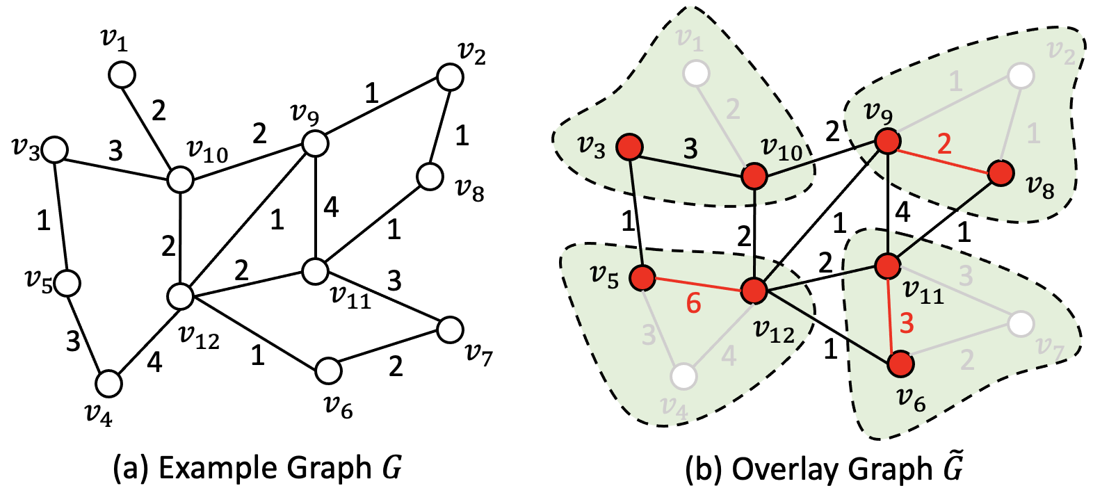
Figure 1: Example Graph $G$ and Overlay Graph $\tilde{G}$

III-A Pre-Boundary Strategy

In this section, we briefly introduce the index construction and query processing of conventional pre-boundary strategy and then propose its index update method.

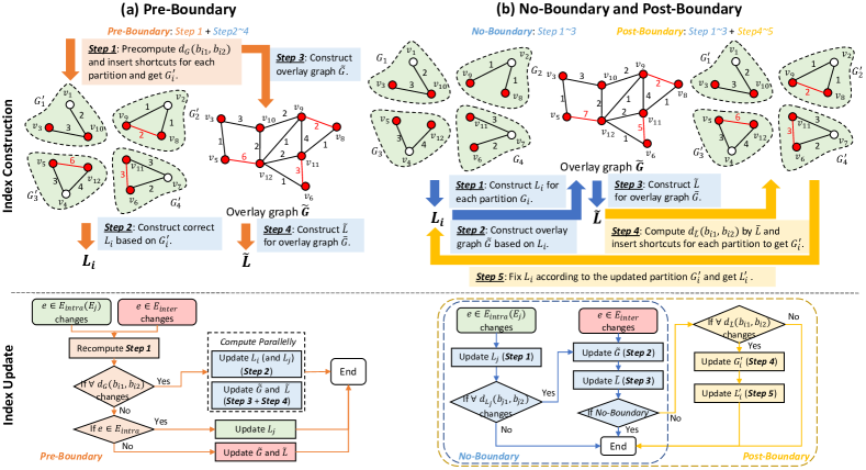
Figure 2: Illustration of Different Partitioned Index Strategies

Index Construction. It consists of four steps (Figure 2-(a)):

Step 1: Precompute the global distance between all boundary vertex pairs $(b_{i1},b_{i2}),(b_{i1},b_{i2}\in B_{i})$ for each partition $G_{i}$ and insert shortcuts $e(b_{i1},b_{i2})=d_{G}(b_{i1},b_{i2})$ into $G_{i}$ to get $G^{\prime}_{i}$;

Step 2: Construct the SP index $L_{i}$ based on $G^{\prime}_{i}$;

Step 3: Construct the overlay graph $\tilde{G}$ based on the precomputed shortcuts in Step 1. Specifically, as shown in Figure 1, $\tilde{G}$ is composed of those boundary vertex pairs $\{B_{i}\times B_{i}\}$ and the inter-edge set $E_{inter}$, that is $V_{\tilde{G}}=\{B_{i}\},E_{\tilde{G}}=\{(b_{i1},b_{i2})\}\cup E_{inter},(b_{i1},b_{i2}\in B_{i})$.

Step 4: Construct the SP index $\tilde{L}$ for $\tilde{G}$.

Note that the construction of $\tilde{L}$ (Step 3, Step 4) can be parallelized with $L_{i}$ (Step 2) since they are independent and both rely on Step 1. All pairs of boundaries are independent of each other so we only need $|B|$ times of Dijkstra’s so this part is $O(nlogn+m)$. Then each partition’s label $L_{i}$ can be constructed in parallel, and $\tilde{L}$’s construction is also independent to them, so its complexity is the worst case of them: $max\{O_{c}(G_{i}),O_{c}(\tilde{G})\}$, where $O_{c}$ is the complexity of underlying index’s construction time as our discussion is not fixed to any specific index structure.

Query Processing. To answer SP query $Q(s,t)$ with index $L$ , we divide the queries into two cases as follows:

Case 1: Two vertices are in the same partition i.e., $\forall s,t\in G_{i}$, $Q(s,t)=d_{L_{i}}(s,t)$.

Case 2: Two vertices are in different partitions, i.e., $\forall s\in G_{i},t\in G_{j}(i\neq j),Q(s,t)=$

$$\begin{cases}d_{\tilde{L}}(s,t)&s,t\in B\\ \min\limits_{b_{q}\in B_{j}}\{d_{\tilde{L}}(s,b_{q})+d_{L_{j}}(b_{q},t)\}&s\in B,t\notin B\\ \min\limits_{b_{p}\in B_{i}}\{d_{L_{i}}(s,b_{p})+d_{\tilde{L}}(b_{p},t)\}&s\notin B,t\in B\\ \min\limits_{b_{p}\in B_{i},b_{q}\in B_{j}}\{d_{L_{i}}(s,b_{p})+d_{\tilde{L}}(b_{p},b_{q})+d_{L_{j}}(b_{q},t)\}&s\notin B,t\notin B\\ \end{cases}$$

In summary, when $s$ and $t$ are in the same $G_{i}$, we can use $L_{i}$ to answer $d_{G}(s,t)$; otherwise, we have to use $L_{i},L_{j}$ and $\tilde{L}$. The intra-query complexity is $O_{q}(L_{i})$, where $O_{q}$ is the index’s query complexity. The inter query is made up of three parallel query sets, and the complexity is the worst of them: $max\{B_{i}\times O_{q}(L_{i}),B_{i}\times B_{j}\times O_{q}(\tilde{L}),B_{j}\times O_{q}(L_{j})\}$.

Index Update. We divide index update into two scenarios:

Scenario 1: Intra-edge weight change. As shown in Figure 2-(a), when $e\in E_{intra}$ ($e\in E_{j}$) changes, we first recalculate Step 1 and compare the old and new weights of $e(b_{i1},b_{i2})$ between boundary in each partition $G_{i}$. If there is any edge weight update, we need to update the corresponding $L_{i}$ and $\tilde{L}$; otherwise, we only need to update $L_{j}$. Note that updates of $L_{i}$ and $\tilde{L}$ can be paralleled too.

Scenario 2: Inter-edge weight change. Same with Scenario 1, when $e\in E_{inter}$ changes, we also recompute Step 1 first. If there is any $d_{G}(b_{i1},b_{i2})$ changes, we update $L_{i}$ and $\tilde{L}$; otherwise, we only need to update $\tilde{L}$.

Lemma 1.

The indexes of Pre-Boundary Strategy can be correctly updated with the above strategy.

Proof.

First of all, we need to recalculate Step 1 to identify the affected edges $e(b_{i1},b_{i2})$ between boundary vertex pairs in each partition. Even though this step is time-consuming, it cannot be skipped since it would be hard to identify the affected edges. For example, suppose the shortest path between the boundary pair $(b_{j1},b_{j2})$ in $G_{j}$ passes through an edge $e\in G_{i}$ with $d_{\tilde{G}}(b_{j1},b_{j2})=d_{0}$. When $e$ increases, we could update $L_{i}$ and then $\tilde{L}$. But $\tilde{L}$ cannot be correctly updated since it could be that $d_{\tilde{G}}(b_{j1},b_{j2})>d_{0}$, such that $d_{\tilde{G}}(b_{j1},b_{j2})$ cannot be refreshed to the correct value. It is because $d_{0}$ contains the old smaller edge weight while cannot be identified, since the shortest distance index always takes the smallest distance value. Then we could select those affected edges $e(b_{i1},b_{i2})$ by comparing their old and new weights. Lastly, we update their corresponding partition index $L_{i}$ and $\tilde{L}$ in parallel. ∎

The Step 1 boundary takes $O(nlogn+m)$ time, while the partition and $\tilde{G}$ index takes $max\{O_{c}(G_{i}),O_{c}(\tilde{G})\}$ time to update in parallel, where $O_{u}$ is the update complexity for different indexes.

TABLE I: Partition Index Strategies Comparison

[] Opeartions Procedure Complexity Pre-Boundary Construction $\{B_{i}\times B_{i}\}\rightarrow\{L_{i}\}\rightarrow L$ $O(nlogn+m)+max\{O_{c}(G_{i}),O_{c}(\tilde{G})\}$ Query Intra $L_{i}$ $O_{q}(L_{i})$ Inter $L_{i}\oplus L\oplus L_{j}$ $max\{B_{i}\times O_{q}(L_{i}),B_{i}\times B_{j}\times O_{q}(\tilde{L})$ $,B_{j}\times O_{q}(L_{j})\}$ Update $\{B_{i}\times B_{i}\}\rightarrow\{L_{i}\}\cup L$ $O(nlogn+m)+max\{O_{u}(G_{i}),O_{u}(\tilde{G}\})$ Post-Boundary Construction $\{L_{i}\}\rightarrow L\rightarrow$ $\{B_{i}\times B_{i}\}\rightarrow\{L_{i}\}$ $max\{O_{c}(G_{i})\}+O_{c}(\tilde{G})$ $+O_{q}(\tilde{G})+max\{O_{u}(G_{i})\}$ Query Intra $L_{i}$ $O_{q}(L_{i})$ Inter $L_{i}\oplus L\oplus L_{j}$ $max\{B_{i}\times O_{q}(L_{i}),B_{i}\times B_{j}\times O_{q}(\tilde{L})$ $,O_{q}(B_{j}\times L_{j})\}$ Update $\{L_{i}\}\rightarrow L\rightarrow$ $\{B_{i}\times B_{i}\}\rightarrow\{L_{i}\}$ $max\{O_{u}(G_{i})\}+O_{u}(\tilde{G})+O_{q}(\tilde{G})$ $+max\{O_{u}(G_{i})\}$ No-Boundary Construction $\{L_{i}\}\rightarrow L$ $max\{O_{c}(G_{i})\}+O_{c}(\tilde{G})$ Query Intra $L_{i}\oplus L\oplus L_{i}$ $max\{B_{i}\times O_{q}(L_{i}),B_{i}\times B_{i}\times O_{q}(\tilde{L}))\}$ Inter $L_{i}\oplus L\oplus L_{j}$ $max\{B_{i}\times O_{q}(L_{i}),B_{i}\times B_{j}\times O_{q}(\tilde{L})$ $,B_{j}\times O_{q}(L_{j})\}$ Update $\{L_{i}\}\rightarrow L$ $max\{O_{u}(G_{i})\}+O_{u}(\tilde{G})$ Because different index structures have different complexities but sharing the same input size and logical procedure, we use the following notations to represent the logical complexities: $O_{c}$ is the index construction complexity, $O_{q}$ is the query complexity, and $O_{u}$ is the index update complexity.

III-B No-Boundary Strategy

The first step of the Pre-Boundary could be very time-consuming because only the index-free SP algorithms like Dijkstra’s [18] or A^∗ [19] could be utilized. The index construction and maintenance efficiency suffer when the graph has numerous boundary vertex pairs. Nevertheless, as previously analyzed, it appears to be an essential requirement for constructing the “correct” PSP index. To break such a misconception, we propose a novel No-Boundary strategy which significantly reduces the index construction/maintenance time by skipping the boundary pre-computation step.

Index Construction. It contains three steps (Figure 2-(b)):

Step 1: Construct the shortest distance index $L_{i}$ for each $G_{i}$;

Step 2: Construct the overlay graph $\tilde{G}$ based on $L_{i}$;

Step 3: Construct the shortest distance index $\tilde{L}$ for $\tilde{G}$.

Since the partition indexes $\{L_{i}\}$ are constructed in parallel first and the $\tilde{L}$ is constructed next, the No-Boundary takes $max\{O_{c}(G_{i})\}+O_{c}(\tilde{G})$ in index construction.

Query Processing. As discussed previously, $L_{i}$ cannot answer $G_{i}$’s query correctly, so how can No-Boundary answers correctly? Before giving the answer, we first prove that although $\tilde{L}$ is built upon $\{L_{i}\}$, its correctness for the shortest distance between any two boundary vertices still holds.

Theorem 1.

$\forall s,t\in B,d_{G}(s,t)=d_{\tilde{L}}(s,t)$.

Proof.

We divide all the scenarios into three cases, as shown in Figure 3-(a), and prove them in the following:

Case 1: $s$ and $t$ belong to the same $G_{i}$ and $p_{G}(s,t)$ only passes through the interior of $G_{i}$. Then $d_{G}(s,t)=d_{G_{i}}(s,t)$ and $(s,t)\in\tilde{G}$. Since $\tilde{w}(s,t)=d_{G_{i}}(s,t)$ was used in $\tilde{G}$’s construction, it is obvious that $d_{G}(s,t)=d_{\tilde{G}}(s,t)=d_{\tilde{L}}(s,t)$;

Case 2: $s\in G_{i}$ and $t\in G_{i}$ but $p_{G}(s,t)$ goes outside;

Case 3: $s\in G_{i}$ and $t\in G_{j}$ from different partitions.

For Cases 2 and 3, we take the concise form of $p_{G}(s,t)$ by extracting only the boundary vertices as $p_{c}=\left<s,b_{0},b_{1},\dots,b_{n},t\right>$ ($b_{i}\in B,0\leq i\leq n$). For two adjacent vertices $b_{i},b_{j}\in p_{c}$, 1) if $b_{i}$ and $b_{j}$ are in the same partition, then its correctness is the same as the sub-case 1; 2) if $b_{i}$ and $b_{j}$ are in different partitions, then $(b_{i},b_{j})$ is an inter-edge with $(b_{i},b_{j})\in\tilde{G}$ and it is naturally correct. Therefore, the shortest distance can be correctly calculated by accumulating only the edge weights on $\tilde{G}$, so $\tilde{L}$ is correct. ∎

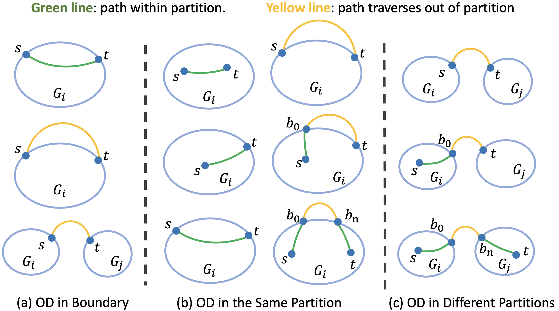
Figure 3: Different Categories of OD Distribution

Based on Theorem 1, we can answer the shortest distance queries of No-Boundary by following strategies:

Case 1: Two query nodes are in the same partition $G_{i}$, i.e., $s,t\in G_{i}$, we report $Q(s,t)$ according to Lemma 2.

Lemma 2.

$\forall s,t\in G_{i}$, $d_{G}(s,t)$ $=\min\{d_{L_{i}}(s,t),$ $\min\{$ $d_{L_{i}}(s,b_{i1})$ $+d_{\tilde{L}}(b_{i1},b_{i2})+d_{L_{i}}(b_{i2},t)\}\}$, where $b_{i1},b_{i2}\in B_{i}$.

Proof.

We denote $d_{L_{i}}(s,t)$ as $d_{2}$, $\min\{d_{L_{i}}(s,b_{i1})+d_{\tilde{L}}(b_{i1},b_{i2})+d_{L_{i}}(b_{i2},t)\}$ as $d_{4}$, and divide all the scenarios into two cases:

Case 1: $p_{G}(s,t)$ does not go outside of $G_{i}$, as shown in the left side of Figure 3-(b). In fact, no matter $s$ and $t$ are boundary vertices or not, $d_{L_{i}}(s,t)$ (i.e., $d_{2}$) is enough to answer $d_{G}(s,t)$ as $L_{i}$ is built based on $G_{i}$ and $G_{i}$ contains all necessary information for finding the shortest path.

Case 2: $p_{G}(s,t)$ passes outside of $G_{i}$, as shown in the right side of Figure 3-(b). If $s$ and $t$ are both boundary vertices, $d_{G}(s,t)=d_{\tilde{L}}(s,t)$ and thus Lemma 2 holds by referring to Theorem 1. If $s$ and $t$ are both non-boundary vertices, we take the concise form of $p_{G}(s,t)$ by extracting only the boundary vertices as $p_{c}=\left<s,b_{0},b_{1},\dots,b_{n},t\right>$ ($b_{i}\in B,0\leq i\leq n$). Therefore, $d_{4}$ can correctly deal with this case as the $d_{G}(b_{0},b_{n})$ can be answered by $d_{\tilde{L}}(b_{0},b_{n})$ according to Theorem 1, while $d_{G}(s,b_{0})$ and $d_{G}(b_{n},t)$ can be answered by $d_{L_{i}}(s,b_{0})$ and $d_{L_{i}}(b_{n},t)$ by referring to Case 1. If either $s$ or $t$ are non-boundary vertex, its distance is the special case of $d_{4}$ and can be easily proved. ∎

Case 2: Two query nodes are in different partitions, i.e., $s\in G_{i},t\in G_{j},i\neq j$, we report $Q(s,t)$ according to Lemma 3.

Lemma 3.

$\forall s\in G_{i},t\in G_{j}(i\neq j),d_{G}(s,t)=$

$$\begin{cases}d_{\tilde{L}}(s,t)&s,t\in B\\ \min\limits_{b_{q}\in B_{j}}\{d_{\tilde{L}}(s,b_{q})+d_{L_{j}}(b_{q},t)\}&s\in B,t\notin B\\ \min\limits_{b_{p}\in B_{i}}\{d_{L_{i}}(s,b_{p})+d_{\tilde{L}}(b_{p},t)\}&s\notin B,t\in B\\ \min\limits_{b_{p}\in B_{i},b_{q}\in B_{j}}\{d_{L_{i}}(s,b_{p})+d_{\tilde{L}}(b_{p},b_{q})+d_{L_{j}}(b_{q},t)\}&s\notin B,t\notin B\\ \end{cases}$$

Proof.

We prove it according to the following cases:

Case 1: Both $s$ and $t$ are boundary vertices. It is correct according to Theorem 1.

Case 2: Either $s$ or $t$ is a boundary vertex. Suppose $s$ is an inner vertex of $G_{i}$ and $t$ is a boundary vertex, as shown in Figure 3-(c). We take the concise $p_{s,t}$ by extracting the boundary vertices as $p_{c}=\left<s,b_{0},\dots,b_{n},t\right>$. Then $b_{0}\in B_{i}$ and $p_{s,t}$ can be treated as concatenated by two sub-paths $p_{s,b_{0}}\oplus p_{b_{0},t}$. Specifically, $d_{G}(s,b_{0})=d_{L_{i}}(s,b_{0})$ by referring to Case 1 here, and $d_{G}(b_{0},t)=d_{\tilde{G}}(b_{0},t)=d_{\tilde{L}}(b_{0},t)$ by referring to Theorem 1.

Case 3: Neither $s$ nor $t$ is a boundary vertex. It can be proved by extending Case 2. ∎

In summary, when $s$ and $t$ are both boundary vertices, we can use $\tilde{L}$ to answer $d_{G}(s,t)$; otherwise, we have to use $L_{i},L_{j}$ and $\tilde{L}$. The intra-query complexity is $max\{O_{q}(L_{i}),B_{i}\times B_{j}\times O_{q}(\tilde{L}),B_{j}\times O_{q}(L_{j})\}$, while the inter-query takes $O_{q}(\tilde{L})$ time when $s$ and $t$ are both boundary vertices, and the complexity of other case is the worst of them: $max\{B_{i}\times O_{q}(L_{i}),B_{i}\times B_{j}\times O_{q}(\tilde{L}),B_{j}\times O_{q}(L_{j})\}$.

Index Update. We divide index update into two scenarios:

Scenario 1: Intra-edge weight change. As shown in Figure 2-(b), when $e\in E_{intra}$ ($e\in E_{j}$) changes, we first update $L_{j}$ and compare the old and new weights of $e(b_{j1},b_{j2})$ between boundary in $G_{j}$. If there is an edge weight update, we need to further update $\tilde{L}$.

Scenario 2: Inter-edge weight change. When $e\in E_{inter}$ changes, only $\tilde{L}$ needs update.

Lemma 4.

The indexes of No-Boundary can be correctly maintained with the above update strategy.

Proof.

In the inter-edge update case, since $e\in\tilde{G},e\notin G_{i},\forall e\in E_{inter}$, the weight change of $e$ could only affect the correctness of $\tilde{L}$. So only $\tilde{L}$ should be checked and updated. In the Intra-edge update case, since $e\in G_{i}$, its weight change will firstly affect $L_{i}$. Then it could affect $\tilde{G}$ as $e_{\tilde{G}}(b_{il_{1}},b_{il_{2}})=d_{L_{i}}(b_{il_{1}},b_{il_{2}})$. So $\tilde{L}$ also needs update if $e_{\tilde{G}}(b_{il_{1}},b_{il_{2}})$ changes after checked. ∎

The update complexity is $max\{O_{u}(G_{i})\}+O_{u}(\tilde{G})$.

III-C Post-Boundary Strategy

Since the time complexity of query processing in No-Boundary is worse than Pre-Boundary, could we accelerate it? We solve this question by propose novel Post-Boundary strategy which utilizes $\tilde{L}$ to fix the incorrect boundary pairs of $G_{i}$ and fix $L_{i}$, thus achieving efficiency query processing.

Index Construction. There are 5 steps for index construction and the first three steps are identical with No-Boundary, adding two steps for post-processing (Figure 2-(b) yellow).

Step 1-3: Same with No-Boundary (see Section III-B).

Step 4: Compute $d_{\tilde{L}}(b_{i1},b_{i2})$ by $\tilde{L}$ for each partition $i$, and insert shortcuts $e(b_{i1},b_{i2})=d_{\tilde{L}}(b_{i1},b_{i2})$ into $G_{i}$ to get $G^{\prime}_{i}$;

Step 5: Fix $L_{i}$ using the updated partition $G^{\prime}_{i}$, denoted as $L_{i}^{\prime}$.

Query Processing. Since $L_{i}^{\prime}$ is correct, the query processing of Post-Boundary is the same as the Pre-Boundary by using $\tilde{L}$ together with $\{L_{i}^{\prime}\}$.

Index Update. It is similar to No-Boundary, with an additional judgment and processing as shown in Figure 2-(b).

Scenario 1: Intra-edge weight change. Suppose $e\in E_{i}$ changes, we update $G_{i},L_{i}$ and then update $\tilde{G},\tilde{L}$ if any $d_{L_{j}}(b_{j1},b_{j2})$ changes. After that we may need to further update $\{G^{\prime}_{i}\},\{L^{\prime}_{i}\}$ if $d_{G_{i}^{\prime}}(d_{i1},d_{i2})$ and $d_{\tilde{L}}(d_{i1},d_{i2})$ are different.

Scenario 2: Inter-edge weight change. Suppose $e\in E_{inter}$ changes, we update $\tilde{G},\tilde{L}$ and then update $\{G_{i}^{\prime}\},\{L_{i}^{\prime}\}$.

Lemma 5.

The indexes of Post-Boundary Strategy can be correctly maintained with the above update strategy.

Proof.

Firstly, we prove the necessity to keep both $\{G_{i}\},\{L_{i}\}$ and $\{G_{i}^{\prime}\},\{L_{i}^{\prime}\}$. Similarly to the Pre-Boundary Strategy, those boundary edges in $\{G_{i}^{\prime}\}$ would keep the old smaller value such that the index could not be correctly updated as explained in Lemma 1. So keeping $\{G_{i}\},\{L_{i}\}$ gives us a chance to update $\tilde{L},\{L_{i}\}$ correctly as proved in Lemma 4. Then, following the No-Boundary Strategy update, we recompute the shortest distance between the all-pair boundaries leveraging $\tilde{L}$ and compare their values on $L_{i}^{\prime}$, then update $G_{i}^{\prime},L_{i}^{\prime}$. ∎

Therefore, the update time complexity is the linear combination of the above procedures: $max\{O_{u}(G_{i})\}+O_{u}(\tilde{G})+O_{q}(\tilde{G})+max\{O_{u}(G_{i})\}$. The time complexities of these three partitioned index strategies are summarized in Table I.

As shown in the index construction part of Figure 2, Pre-Boundary precomputes the all-pair shortest distance among boundary vertices of each partition, and thus the newly added shortcuts of $G_{i}$ and $\tilde{G}$ (red edges) are of correct edge weight. For example, the edge weight of $e(v_{5},v_{12})$ is 6 which is the path length of the shortest path $p_{G}(v_{5},v_{12})=\left<v_{5},v_{3},v_{10},v_{12}\right>$. While No-Boundary and Post-Boundary only leverage $L_{i}$ to construct the shortcuts for overlay graph $\tilde{G}$, and thus the edge weight of shortcut $e(v_{5},v_{12})$ is 7 which preserves the distance of path $p_{G_{3}}(v_{5},v_{12})=\left<v_{5},v_{4},v_{12}\right>$. Moreover, Post-Boundary utilizes $\tilde{L}$ to get the shortest distance of boundary pairs of each partition and insert the shortcuts to get $G^{\prime}_{i}$ (e.g., insert $e(v_{5},v_{12})=6$ to $G^{\prime}_{3}$). Therefore, Post-Boundary has the same efficiency as Pre-Boundary in processing the query pairs within the same partition, which is faster than No-Boundary.

Balance Discussion: There exists a balance of index performance among the three variants mentioned above. In terms of the query processing, the No-Boundary is slower than both Pre-Boundary and Post-Boundary, since the boundary vertices and path concatenation should be considered for OD within one partition. In terms of the index update, the No-Boundary and Post-Boundary enjoy faster speed as the boundary all-pair distance can be neglected. In terms of the index size, the Post-Boundary needs twice the storage space as that of No-Boundary and Pre-Boundary, even though it has advantages in both query processing and index update. Therefore, no one strategy is better than the others in all aspects and could be selected based on the application scenario.

III-D Pruned-Boundary Optimization

As analyzed previously, the density of $\tilde{G}$ increases dramatically as the all-pair boundary vertices in each partition are connected during construction. Moreover, the high density could affect the index performance [8] by slowing down the index construction, query processing, and index update. Then is it possible to decrease the density of $\tilde{G}$ by deleting some edges in $\{B_{i}\times B_{i}\}$? As proved in Theorem 1, the shortest distance between boundary vertices is well-preserved in $\tilde{G}$, then could the distance still be preserved in $\tilde{G}$ if some edges are removed? In the following, we start by considering the connectivity of boundary vertices and define them accordingly:

Definition 4 (Half/Full-Connected Boundary Vertex).

In $G_{i}$, $b_{p}\in B_{i}$ is a half-connected boundary vertex if $\exists u\in N(b_{p}),u\in G_{i},u\notin B_{i}$ and we denote them as $B_{i}^{H}$; otherwise, $b_{p}$ is a full-connected boundary vertex and denoted as $B_{i}^{F}$.

Intuitively, $\forall b_{p}\in B_{i}^{F}$, the first edge on its shortest path to other boundary vertices in $B_{i}$ only leads to another boundary vertex according to the Definition 4. Thus the edges between $b_{p}$ and its neighbors seem enough to preserve $b_{p}$’s connections to other boundary vertices $B_{i}\backslash b_{p}$. Whereas for $b_{q}\in B_{i}^{H}$, it is insufficient to only include the edges between $b_{q}$ and its boundary neighbors in $\tilde{G}$ since its shortest path to other boundary vertices could also pass through its non-boundary neighbors. Therefore, we propose to shrink $\tilde{G}$ to $\tilde{G^{\prime}}$ by taking the edges between half-connected boundary vertices $B_{i}^{H}\times B_{i}^{H}$ and the adjacent edges of full-connected boundary vertices.

Lemma 6.

$d_{G_{i}}(b_{s},b_{t})=d_{\tilde{G_{i}^{\prime}}}(b_{s},b_{t})$, $\forall(b_{s},b_{t})\in B_{i}\times B_{i}$.

Proof.

Since $d_{G_{i}}(b_{s},b_{t})=d_{\tilde{G_{i}}}(b_{s},b_{t})$ holds with $e_{\tilde{G_{i}}}(b_{s},b_{t})=d_{G_{i}}(b_{s},b_{t})$ and $E_{\tilde{G^{\prime}_{i}}}\subset E_{\tilde{G_{i}}}$, it should be that $d_{\tilde{G_{i}}}(b_{s},b_{t})\leq d_{\tilde{G^{\prime}_{i}}}(b_{s},b_{t})$, that is $d_{G_{i}}(b_{s},b_{t})\leq d_{\tilde{G^{\prime}_{i}}}(b_{s},b_{t})$. Then our next step is to prove that $d_{\tilde{G^{\prime}_{i}}}(b_{s},b_{t})\leq d_{G_{i}}(b_{s},b_{t})$. We categorize the combination of $b_{s}$ and $b_{t}$ into three types:

Case 1: $b_{s},b_{t}\in B^{H}_{i}$. Since $e_{\tilde{G^{\prime}_{i}}}(b_{s},b_{t})=d_{G_{i}}(b_{s},b_{t})$ with $(b_{s},b_{t})\in\tilde{G^{\prime}_{i}}$, it is clear that $d_{G_{i}}(b_{s},b_{t})=d_{\tilde{G_{i}}^{\prime}}(b_{s},b_{t})$.

Before analyzing Case 2 and Case 3, we suppose that the concise form of $p_{G_{i}}(b_{s},b_{t})$ by taking only the boundary vertices is $\{b_{s},b_{0},\dots,b_{k},b_{t}\},(0\leq k)$.

Case 2: $b_{s}\in B^{F}_{i},b_{t}\in B^{H}_{i}$. In the case of $k=0$, it means that $b_{s}\in N(b_{t})$ and $d_{G_{i}}(b_{s},b_{t})=e_{G_{i}}(b_{s},b_{t})$. Since $(b_{s},b_{t})\in\tilde{G_{i}}^{\prime}$ with $e_{\tilde{G^{\prime}_{i}}}(b_{s},b_{t})=e_{G_{i}}(b_{s},b_{t})$, it should be that $d_{G_{i}}(b_{s},b_{t})=d_{\tilde{G^{\prime}_{i}}}(b_{s},b_{t})$. Then in the case of $k>0$, we suppose that the first half-connected boundary vertex on $p_{G_{i}}(b_{s},b_{t})$ is $b_{l}$, that is $b_{j}\in B^{F}_{i}(0\leq j<l),b_{l}\in B_{iH}$. The shortest distance value can be accumulated as $d_{G_{i}}(b_{s},b_{t})=\sum_{j=1}^{l-1}e_{G_{i}}(b_{j-1},b_{j})+d_{G_{i}}(b_{l},b_{t})$. As $b_{j}\in B^{F}_{i}(0\leq j<l)$, then $e_{G_{i}}(b_{j-1},b_{j})=e_{\tilde{G^{\prime}_{i}}}(b_{j-1},b_{j})$ according to the definition 4. And $d_{G_{i}}(b_{l},b_{t})=d_{\tilde{G^{\prime}_{i}}}(b_{l},b_{t})$ by referring to the above Case 1 as $b_{l},b_{t}\in B^{H}_{i}$. So $d_{G_{i}}=\sum_{j=1}^{l-1}e_{\tilde{G^{\prime}_{i}}}(b_{j-1},b_{j})+d_{\tilde{G^{\prime}_{i}}}(b_{l},b_{t})$ holds, which indicates that $d_{\tilde{G^{\prime}_{i}}}(b_{s},b_{t})\leq d_{G_{i}}(b_{s},b_{t})$.

Case 3: $b_{s},b_{t}\in B^{F}_{i}$. Similarly, we suppose that the first half-connected vertex on $p_{G_{i}}(b_{s},b_{t})$ is $b_{l}$. Then $d_{G_{i}}(b_{s},b_{t})=d_{G_{i}}(b_{s},b_{l})+d_{G_{i}}(b_{l},b_{t})\geq d_{\tilde{G^{\prime}_{i}}}(b_{s},b_{l})+d_{\tilde{G^{\prime}_{i}}}(b_{l},b_{t})$ by referring to Case 2 above as $b_{s}\in B^{F}_{i},b_{l}\in B^{H}_{i},b_{t}\in B^{F}_{i}$. So it could also be proved that $d_{\tilde{G^{\prime}_{i}}}(b_{s},b_{t})\leq d_{G_{i}}(b_{s},b_{t})$.

By summarizing the above three cases, $d_{G_{i}}(b_{s},b_{t})=d_{\tilde{G^{\prime}_{i}}}(b_{s},b_{t})$, and the $\tilde{L^{\prime}}$ is also correct. ∎

Therefore, Lemma 6 shows that our index correctness can still be guaranteed after pruned-boundary optimization.

IV Partitioned SP Index Scheme

Having figured out how to deal with boundaries for better index performance (efficient query or quick update), the partition method and SP index are other critical components for PSP index. Among them, the SP index is well studied and analyzed in section II-C. Then, there comes a problem: how could we choose a partition method or which partition method contributes to our preferred performance? This is not trivial because: 1) dozens of partition methods (as seen in section II-B) with different characteristics were proposed and applied in the past decades; 2) they are classified under different criteria while it is not clear which criterion is beneficial to SP index; 3) their relationship with (or the effect on) SP index is unknown and has never been studied. Based on these doubts, we first identify the partition equivalence under existing classification criteria and propose a novel and SP-oriented category of partition methods. Then we establish the PSP index scheme by coupling the partitioned index strategy, partition method, and SP index, and analyze the index complexity under different partition categories.

IV-A Partition Equivalence

According to [48], the existing partition algorithms have many classification methods from the perspectives of partition manners (spectral, flow, graph glowing, contraction and multi-level), partition objectives (balance and minimal cut), computation manner (in-memory, distributed and streaming), and cut category (edge-cut and vertex-cut), etc. Among them, the ones with minimal cut as objective is promising. However, they can still be categorized into edge-cut and vertex-cut further down.

We generalize the vertex-cut to edge-cut by duplicating those vertices which are cut into different partitions and connecting the duplicated vertices with their original vertices through an edge of zero weight. Suppose in a graph $G$, a vertex $x$ is cut into $l+1$ different partitions $\{G_{0},G_{1},\dots,G_{l}\}$ in a vertex-cut partition with $x$ along with its neighbors $\{x_{n_{i}}\}(0\leq i\leq l)$ belonging to subgraph $G_{i}$. To obtain its equivalent edge-cut partition, we transform $G$ to $G^{\prime}$: $\forall$ $x\in X$ (cut vertex set), keep the connection between $x$ and its partial neighbors $\{x_{n_{0}}\}$, duplicate $x$ as $x_{i}$ connecting neighbors $x_{n_{i}}$, and connect $x$ with $x_{i}$ by an edge with $e(x,x_{i})=0$. Then we partition $G^{\prime}$ by using edge-cut partition: cut each added edge $(x,x_{i})$, which leads to the following lemma:

Lemma 7.

The edge-cut partition of $G^{\prime}$ by cutting those added edges $(x,x_{i})$ is equivalent to the vertex-cut partition of $G$ by cutting the vertices in $X$.

Following by, we verify that the partition equivalence has no effect on the shortest distance computation.

Theorem 2.

$\forall s,t\in V,d_{G}(s,t)=d_{G^{\prime}}(s,t)$.

Proof.

We classify all the scenarios into two cases:

Case 1: $p_{G}(s,t)$ ($p_{s,t}$ for short) does not pass through any $x\in X$. It indicates that $p_{s,t}$ is totally within one partition $G_{i}(1\leq i\leq k)$. Since the vertex-cut partition of $G$ and the edge-cut partition of $G^{\prime}$ are equivalent, $d_{G_{i}}(s,t)=d_{G}(s,t)=d_{G^{\prime}}(s,t)$ holds.

Case 2: $p_{s,t}$ pass through $x\in X$. We suppose that $p_{s,t}=\left<s,\dots,x_{f},x,x_{b},\dots,t\right>$ with $x_{f}\in G_{i},x_{b}\in G_{j}$, then it can correspond to $p_{s,t}^{\prime}=\left<s,\dots,x_{f},x_{i},x,x_{j},x_{b},\dots,t\right>$ in $G^{\prime}$. Since $e(x_{i},x)=e(x,x_{j})=0$, $l(p_{s,t})=l(p_{s,t}^{\prime})$ holds which prove that $d_{G}(s,t)=d_{G^{\prime}}(s,t)$ is correct as well. ∎

Even though they are equivalent, their influence on the partitioned index is different in the following two aspects:

1) Boundary Inter-Connection: Firstly, within partitions, they have the same complexity even though the vertex-cut’s partition sizes are slightly larger due to the sharing boundaries. However, in Pre-Boundary and Post-Boundary of the overlay graph, the boundaries of the edge-cut are only fully connected to vertices in one partition, while the vertex-cuts’ boundaries are fully connected to multiple partitions, which makes the graph much denser. Further, due to the equivalence between PLL and tree-decomposition [26], we can use the decomposed tree to estimate the label size. Specifically, due to the ancestor-descendant relations between a vertex and its neighbors (also the ones connected through shortcuts), they will appear on a single branch of the tree. When we use edge-cut, the boundaries can be organized in the unit of partitions and reduce the tree height effectively [17]. However, when we use the vertex cut, the larger neighbor number first prolongs the branch length. What’s worse, the one-boundary-multiple-partition structure prohibits partition-oriented processing. Therefore, the vertex-cut’s label size is more likely to reach the worst-case label size $O(|B|^{2})$, where the tree decays to a stick.

2) Boundary Vertex Number: The second and the most important issue comes with the huge boundary vertex number of the vertex-cut. As discussed previously, the overlay graph construction requires $B_{i}\times B_{i}$ new edges, and the cross-partition query requires $B_{i}\times B_{j}$ combinations. If a vertex-cut creates 10k boundaries for each partition, which is ordinary, then these two numbers would grow to the scale of billions and dramatically deteriorate efficiency.

Figure 4: Partition Results on Example Graph $G$

IV-B SP-Oriented Partitioning Classification

Based on how the networks structures affect the partitioned shortest path index, we propose a new classification of graph partition methods that has three categories: 1) Planar (spectral partitioning [46, 37], graph growing [49], flow-based partitioning [34, 35], node-swapping [62, 63]), 2) Core-Periphery (core-tree [83, 6, 79], sketch [84, 30]), and 3) Hierarchical (HiTi [41], SHARC [24], G-Tree [44], SMOG [71]) from the perspective of the shortest distance application. Firstly, the Planar treats partitions equally on one level:

Definition 5.

(Planar Partitioning). Planar partitioning decomposes a graph $G$ into multiple equally-important subgraphs $\{G_{i}|1\leq i\leq k\}(k\in[2,\infty])$ with 1) $\bigcup_{i\in[1,k]}V(G_{i})=V$, $V(G_{i})\cap V(G_{j})=\emptyset$, or 2) $\bigcup_{i\in[1,k]}E(G_{i})=E$, $E(G_{i})\cap E(G_{j})=\emptyset,\forall i,j\in[1,k],i\neq j$.

The second Core-Periphery Partition [85, 86, 87, 88] treats the partitions discriminately by taking some important vertices as “Core” and the remaining ones as “Peripheries”:

Definition 6.

(Core-Periphery Partitioning). Core-periphery partitioning decomposes a graph $G$ into two distinct parts: a core subgraph $G_{c}$ and $k-1$ peripheral subgraphs $\{G_{i}|1\leq i\leq k-1\}(k\in[2,\infty])$, satisfying $\bigcup_{i\in[1,k-1]}V(G_{i})\cup V(G_{c})=V,V(G_{c})\cap V(G_{i})=\emptyset(\forall 1\leq i\leq k-1)$ and $V(G_{i})\cap V(G_{j})=\emptyset(\forall i,j\in[1,k-1],i\neq j)$.

There are two big streams depending on how the core is formed: 1) Core-Tree Decomposition [83, 6, 79] forms the core through tree decomposition [89], and the resulting periphery part is a set of small-width trees. Specifically, it leverages minimum degree elimination [90] to contract vertices of lower degree first such that the graph is contracted from the edge towards the center, generating a set of growing trees (“Peripheries”) around a shrinking while denser graph (“Core”) formed by those non-contracted vertices. The contraction terminates when the width of one tree reaches the previously set threshold; 2) Sketch [91, 84, 92, 93, 94, 95, 96, 29, 30] selects a set of vertices as landmarks, which can be regarded as the core and treats the remaining parts as periphery. It generally works on extremely large graphs where the above tree decomposition is impossible. The landmarks are used for distance estimation (precomputing landmarks to peripheries) or highways (precomputing index between landmarks).

The third Hierarchical Partitioning organizes the network partitions hierarchically and each level is equivalent to Planar Partitioning (Core-Periphery can also be organized hierarchically [97] but it is essentially organizing the landmarks).

Definition 7.

(Hierarchical Partitioning.) Hierarchical partitioning organizes a graph $G$ hierarchically within $H$ levels where each level $h$ is a planar partitioning $\{G^{h}_{i}\}$ of $G$ and $\exists G^{h-1}_{j}\supset G^{h}_{i},\forall G^{h}_{i}(1\leq h<H)$.

To simplify the presentation, Figure 4 shows the partition results of an example graph $G$ with respect to different partitioning methods, where the red vertices represent the corresponding boundary vertices. Specifically, planar partitioning generates four partitions with equivalent vertex size while core-periphery partitioning produces both “Core” and “Periphery” (Note that the periphery of Core-Tree decomposition is a set of small-width trees while Sketch treats the non-core part as periphery. The yellow vertex in each periphery is the “root vertex”). Hierarchical partitioning organizes partitions hierarchically, and the leaf nodes (the lowest level partition result) may have the same partition result as planar partitioning if the same partitioning method is used.

As analyzed in Section III, the boundary number of each partition is crucial to PSP index. Therefore, we propose the following remark to clarify the relations of these partition methods and how they influence path-finding.

Remark: Boundary Constraint on Partition Choice. The planar and hierarchical partitions have no limit to the boundary number even though reducing the cut size is one of their optimization goals so that the path index may suffer from large boundary numbers. On the other hand, the core-tree decomposition limits the boundary number to be no larger than the pre-defined bandwidth so their performance would not be deteriorated by the boundary if we set the bandwidth wisely. Therefore, the planar and hierarchical partitions are better used for small treewidth networks such that balanced partitions and fewer boundaries can be achieved together. While core-periphery is suitable for large treewidth networks as it deliberately limits the boundary vertex number by bandwidth.

IV-C Coupling Partition Strategy, Index, and Partition Structure

After identifying the three dimensions of partitioned shortest path indexes (partitioned index strategy, path index, partition structure), now we are ready to couple them together to assemble various indexes to satisfy different scenarios. We organize and illustrate them in Figure 5-(a). Specifically, we order the strategies and indexes based on their efficiency on query and update (other factors like construction time and space consumption are omitted), and we can obtain a PSP index by choosing one from each category and have a rough idea of its performance. It should be noted that all the existing PSP indexes can find their position in it as discussed in Section VI and most of them are query-oriented, while there leaves a vast space of combinations to generate “new” indexes. Although we are able to enumerate them all, in the following, we choose to introduce the representative ones from the perspectives of query-oriented and update-oriented of each partition structure as examples of how to couple the strategies and indexes. Although they are all new structures proposed in this work, we only analyze their components and performance but do not present the details due to the page limit.

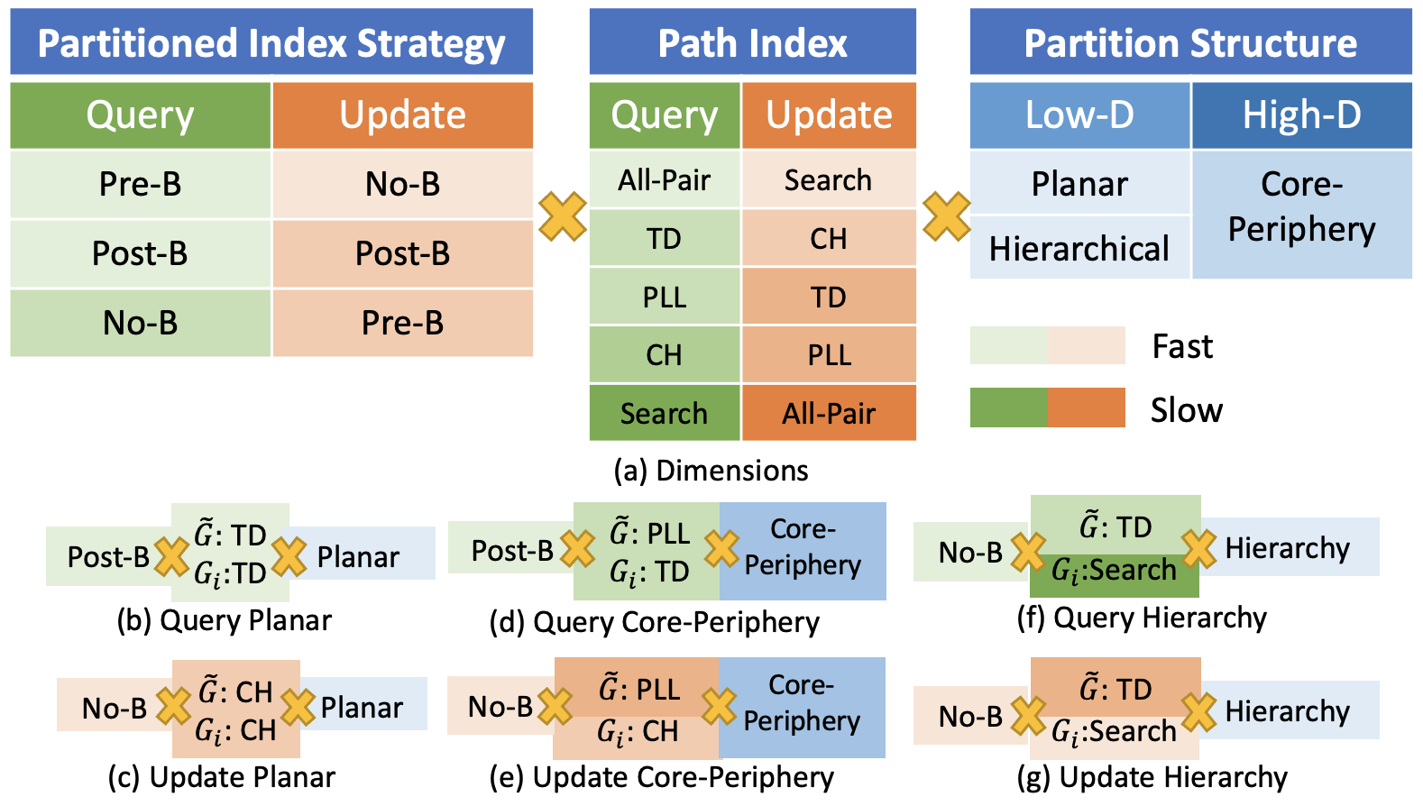
Figure 5: Dimensions of PSP Index Scheme and Representative Coupling

IV-D Coupled Planar Partition Index

Given a planar partition, the partition strategies can apply directly to it. Next, we introduce how to construct the PSP indexes that are efficient for query or index update.

IV-D1 Query-Oriented Planar SP Index

Firstly in terms of partitioned index strategy, Pre-Boundary and Post-Boundary are efficient in query answering, with all the existing works relying on the Pre-Boundary. Since our proposed Post-Boundary is faster than Pre-Boundary in index construction, we used it as the partitioned index strategy. Secondly, in terms of path index, we could choose TD as the index for both partitions and overlay graph. Although all-pair is faster, its space consumption is intolerable. Its structure is shown in Figure 5-(b), and we elaborate its procedures below:

Construction. It takes $O(V_{max}\cdot(\log V_{max}+h_{max}\cdot w_{max}))$ time for the partition TD, $O(V_{\tilde{G}}(\log V_{\tilde{G}}+h_{\tilde{G}}\cdot w_{\tilde{G}}))$ for the overlay TD, $O(B^{2}_{max}w_{\tilde{G}})$ for boundary correction, and $O(w_{\tilde{G}}+w^{2}_{max}\cdot\delta)$ for the partition TD update, where $\delta$ is the affected shortcut number and $max$ are the corresponding max values in the partitions.

Query. The intra-query takes $O(w_{max})$ as partition index is correct, and the inter-query takes $O(max\{B_{max}w_{max},B^{2}{max}w_{\tilde{G}}\})$ for the partition and overlay query and $O(B^{2}_{max})$ for the combinations.

Update. It takes $O(w^{2}_{max}\delta)$ to update partition TD, $O(w^{2}_{\tilde{G}}\delta)$ to update overlay TD, and $O(B^{2}_{max}w_{\tilde{G}})$ to check boundaries.

IV-D2 Update-Oriented Planar SP Index

In terms of the partitioned index strategy, we use No-Boundary as it requires the least effort to update. In terms of indexes, we can choose CH as the underlying index as it is fast to update while the query processing is better than direct search (Figure 5-(c)).

Construction. It is faster with $O(V_{max}\cdot w^{2}_{max}\cdot\log V_{max})$ for partition CH and $O(V_{\tilde{G}}\cdot w^{2}_{\tilde{G}}\cdot\log V_{\tilde{G}})$ for overlay CH.

Query. The query time is longer with $O(max\{B_{max}\cdot w_{max}\log V_{max},$ $B^{2}_{max}\cdot w_{\tilde{G}}\log V_{\tilde{G}}\})$ for the intra- and overlay searching, and $O(B^{2}_{max})$ for the combinations.

Update. It is faster with $O(\delta w_{max})$ for partition CH maintenance and $O(\delta w_{\tilde{G}})$ for overlay CH maintenance.

IV-E Coupled Core-Periphery Partition Index

The core-periphery partition index comprises the core index $L_{c}$ and the periphery index $\{L_{i}\}$. It seems that $L_{c}$ and $L_{i}$ can be constructed by their corresponding subgraphs $G_{c}$ and $G_{i}$, respectively. Although the core does not belong to any partition, they are connected to the partitions, and we treat the core as the overlay graph. As for the two kinds, core-tree is suitable for general-size high-degree networks where indexes are still constructible, while sketch is used on networks with billions of vertices. Different from the previous planar partition, the core here usually has a large degree so its index is limited to PLL. As for sketch, we omit it here because its PLL core + pruned direct search seems to be the only solution for huge networks. Next, we discuss the remaining parts.

IV-E1 Query-Oriented Core-Tree SP Index

For the strategy, the query-oriented still uses the Post-Boundary as the queries within the periphery can be handled without the core index. The periphery index uses TD because the periphery usually has a small degree. This structure is shown in Figure 5-(d).

Construction. Because periphery is constructed through contraction, we regard it as a by-product of the partition phase and do not construct their labels in the first step. Then it takes $O(w_{c}E_{c}\log V_{c}+w^{2}_{c}V_{c}\log^{3}V_{c})$ for the core PLL, $O(B^{2}_{max}w_{c}\log V_{c})$ for boundary correction, and $O(V_{max}\cdot w^{2}_{max}\cdot\log V_{max})$ for periphery label.

Query. The intra-query takes $O(w_{max})$ time. The inter-query takes $O(max\{B_{max}w_{max},B^{2}_{max}w_{c}\log V_{c}\})$ for the periphery and core, and $O(B^{2}_{max})$ for the combinations.

Update. It takes $O(w^{2}_{max}\cdot\delta)$ for the periphery TD, $O(w_{c}E_{c}\log V_{c})$ for the core PLL, and $O(B^{2}_{max}w_{c}\log V_{c})$ for boundary correction.

IV-E2 Update-Oriented Core-Tree SP Index

As shown in Figure 5-(e), No-Boundary is still used as the boundary strategy, while CH is used for faster periphery update.

Construction. Only core needs $O(w_{c}E_{c}\log V_{c}+w^{2}_{c}V_{c}\log^{3}V_{c})$ time.

Query. The query time is longer with $O(max\{B_{max}w_{max}\log V_{max},$ $B^{2}_{max}w_{c}\log V_{c}\})$ for intra and core, and $O(B^{2}_{max})$ for combinations.

Update. It is faster with $O(\delta w_{max})$ for periphery shortcuts and $O(w_{c}E_{c}\log V_{c})$ for the core PLL.

IV-F Coupled Hierarchical Partition Index

This category organizes $L$ levels of partitions hierarchically with several lower partitions forming a larger partition on the higher level. We use $L^{l}_{i}$ to denote the index of partition $G^{l}_{i}$ on level $l$. Different from the state-of-the-art G-Tree stream of indexes which uses all-pair in their hierarchical overlay graph, we replace it with the hierarchical labels for better query and update performance. Specifically, for vertices in each layer, we store their distance to vertices in their upper layers. As this is essentially 2-hop labeling, we use TD to implement it with orderings corresponding to the boundary vertex hierarchy. Such a replacement in the overlay index could answer queries and update much faster than the original dynamic programming-based layer all-pair index.

IV-F1 Update / Query-Oriented Hierarchical Index

As for the partitions, this structure tends to generate partitions with small sizes so we inherit the original search for fast query processing. Consequently, no partition index leads to inevitable boundary all-pair searches. Fortunately, our No-Boundary restricts the search space to the small partition compared with G-Tree’s whole graph Pre-Boundary (Figure 5-(f) and (g)).

Construction. The partition boundary all-pair takes $O(B_{max}\cdot V_{max}(logV_{max}+E_{max}))$, and its by-product boundary-to-partition can be cached for faster inter-query. Then the overlay TD takes $O(V_{\tilde{G}}(logV_{\tilde{G}}+h_{\tilde{G}}w_{\tilde{G}}))$ time.

Query. The intra-query takes $O(B_{max}V_{max}(logV_{max}+E_{max})$ for the direct search (very rare as the partitions are small), while the inter-query The query takes $O(B_{max}w_{\tilde{G}}\})$ for intra- (constant time with cache) and hierarchical query, and $O(B^{2}_{max})$ for combination.

Update. It takes $O(B_{max}\cdot V_{max}(logV_{max}+E_{max}))$ to update the partition all-pairs and $O(w^{2}_{\tilde{G}}\cdot\delta)$ to update the overlay graph.

V Experimental Evaluation

In this section, we evaluate the proposed methods. All the algorithms are implemented in C++ with full optimization on a server with 4 Xeon Gold 6248 2.6GHz CPUs (total 80 cores / 160 threads) and 1.5TB memory.

TABLE II: Dataset Description

[] Type Name Dataset $|V|$ $|E|$ Road Network NY ¹ New York City 264,346 730,100 FL ¹ Florida 1,070,376 2,687,902 W ¹ Western USA 6,262,104 15,119,284 Complex Network GO ² Google 855,802 8,582,704 SK ³ Skitter 1,689,805 21,987,076 WI ³ Wiki-pedia 3,333,272 200,923,676 [1] http://www.dis.uniroma1.it/challenge9/download.shtml

[2] http://snap.stanford.edu/data [3] http://konect.cc/

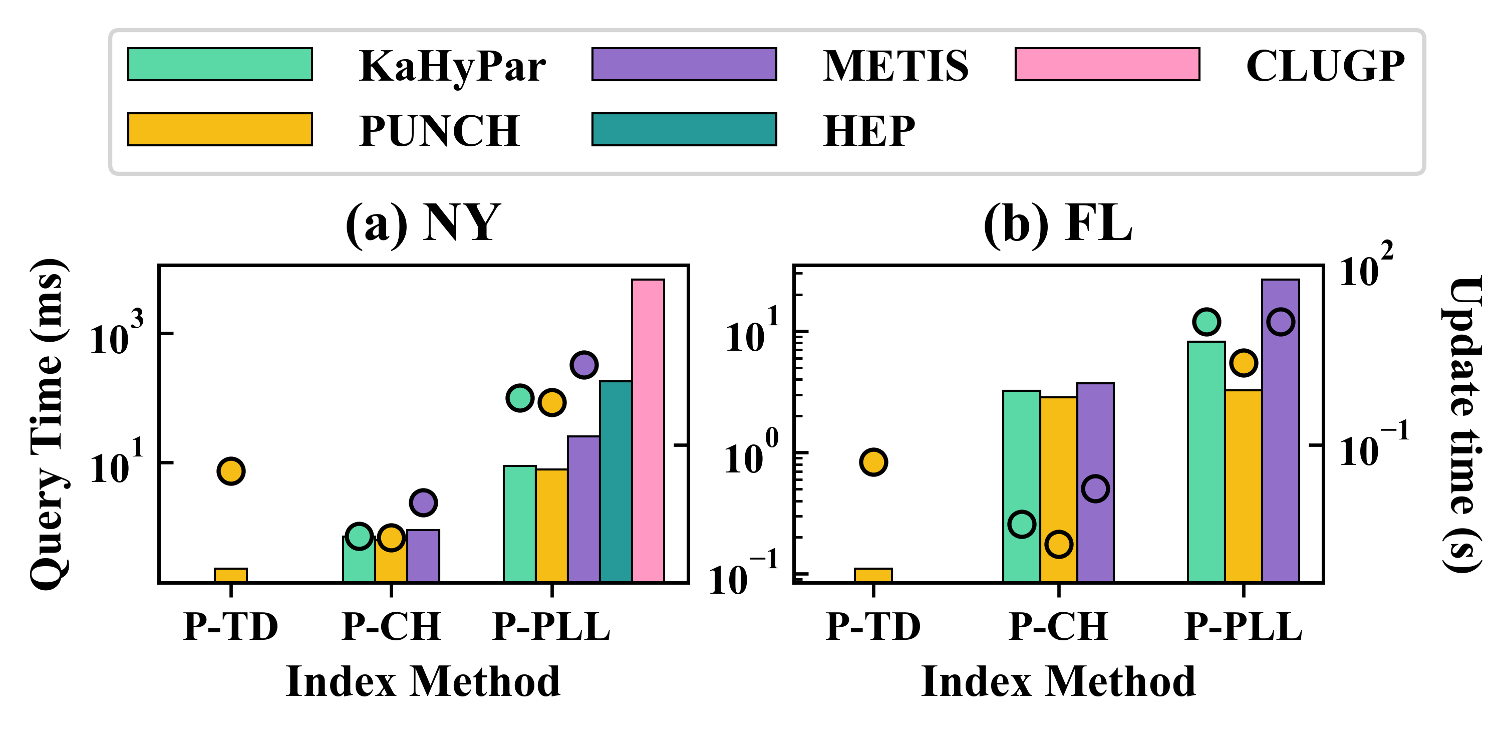
Figure 6: Effect of Graph Partition Methods. Bar: Query, Ball: Update

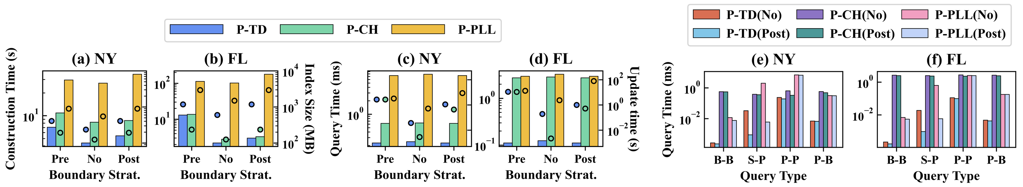
Figure 7: Effect of Partitioned Index Strategy. (For (a)-(d), Bar: Construction Time and Query; Ball: Index Size and Update)

TABLE III: Average Vertex Degree of Overlay Graph

Dataset	NY		FL		GO		SK
Method	PUNCH	HEP	PUNCH	HEP	KP	HEP	KP	HEP
No-Prune	48.68	325.98	36.17	719.25	947.36	9754.52	1420.18	34889.5
Prune	48.68	320.61	36.17	714.30	912.24	7678.05	1409.98	27326.5

V-A Experimental Settings

Datasets and Queries. We test on 3 weighted road networks and 3 complex networks (Table II). In particular, we follow [10] to generate the edge weights for unweighted complex networks in a manner that is inversely proportional to the highest degree of the endpoints. We randomly generate 10,000 queries and 1,000 update instances for each dataset to assess the query processing and index maintenance efficiency, respectively.

Algorithms. We compare with three state-of-the-art baselines from the three partition structures: 1) Forest Label (FHL) [16, 17] belonging to Pre-Boundary + TD/TD + Planar, 2) Core-Tree (CT) [6, 79] belonging to No-Boundary + TD/PLL + Core , and 3) G-Tree [43, 45] belonging to Pre-Boundary + All-Pair + Hierarchy. We implement the five new couplings (Section IV) and name them: Q-Planar, U-Planar, Q-Core, U-Core, and UQ-Hier, with Q and U denoting the Query- and Update-orient. We also implement the partitioned index for TD, CH, and PLL (denoted as P-TD, P-CH, and P-PLL). The default thread number of all methods is set to 150.

Parameter Setting. According to our preliminary results, we set the partition number to $64$ for planar method, while the bandwidth of core-periphery methods are set to $20$. As for hierarchical index, we follow the setting of G-tree, setting the fan-out $f$ as $4$ and the maximum leaf node size $\tau$ as 128 (NY), 256 (FL), and 512 (W). In addition, for each graph, we set one vertex order for the methods with the same partition structure and apply it in all experiments to guarantee fairness.

Performance Metrics. We measure the performance of shortest path method from four aspects: index construction time $t_{c}$, query time $t_{q}$, update efficiency $t_{u}$, and index size $s$.

V-B Performance Comparison

Exp 1: Effect of Partition Method. We first test the five best partition methods for planar index structure (KaHyPar [33], PUNCH [35], METIS [40], HEP [74] and CLUGP [68]). Because P-TD requires partition to be a connected [27], only PUNCH can be used for it. As shown in Figure 6, PUNCH outperforms others in query and update because it reduces the boundary number spatially, whilst vertex-cuts (HEP and CLUGP) perform worse because they generate much more boundaries. As evidenced by both theoretical analysis and experimental results, vertex-cut is worse than edge-cut for partition-based pathfinding. As for the hierarchical partitioning, we follow G-Tree and use its integrated METIS.

Exp 2: Effect of Partitioned Index Strategy. We evaluate different partitioned index strategies on NY and FL. As shown in Figure 7 (a)-(d), the No-Boundary has the lowest construction time ($6\times$ speed-up for P-TD and P-CH), smallest index size, and lowest update time ($73\times$ and $5420\times$ speed-up for P-TD and P-CH) with slightly worse performance on query time. The Post-Boundary has the same query time as Pre-Boundary, a shorter construction time and update time than Pre-Boundary in most cases. We next compare the efficiency of different query types (OD pair are both boundaries (B-B), same partition (S-P), different partitions (P-P), and one boundary one partition (P-B)) for No-Boundary and Post-Boundary strategies. Figure 7 (e)-(f) shows that the Post-Boundary can greatly improve the S-P query ($37\times$ and $19\times$ speed-up for P-TD) while it has almost the same performance with No-Boundary in other types. The performance gain comes from the Post-Boundary’s correct shortcuts. Finally, we evaluate the effectiveness of Pruned-Boundary optimization by measuring the average vertex degree of the overlay graph. We use PUNCH and KaHyPar as the representatives of edge-cut on road networks and complex networks, while HEP for vertex-cut. As shown in Table III, the degree decreases with the Pruned-Boundary in most cases. However, it cannot improve PUNCH as PUNCH already has a very good partition result.

Exp 3: Comparison of Partitioned SP Index Methods. We compare our proposed PSP indexes with the state-of-the-art and the non-partitioned indexes in Figure 8. We first analyze the performance of our proposed indexes against their counterparts: 1) Q-Planar has the same query performance and index size with FHL, but it is faster to construct and update ($84\times$ in W); 2) U-Planar is slower to query, but it is much faster to construct ($8.6\times$ in FL) and update (more than $1000\times$ in all) with smaller index size; 3) UQ-Hier has faster construction, smaller index, faster query and update than G-Tree; 4) Q-Core has longer construction and update time than CT, and it seems to have similar query performance. This is because the query improvement lies in the S-P query type but not the others, and it is the number of S-P query that determines the overall improvement; 5) U-Core has faster construction time, smaller index and faster update than CT, but its query is slower; 6) Sketch can scale up to very large graphs, but its query and update efficiency are slower than Q-Core and U-Core. Note that CT, Q-Core and U-Core cannot finish computation on WI due to insufficient memory, which is caused by “Curse of Pruning Power” of PLL [10] and the denser contracted core graph.

Secondly, we have the following observations: 1) Partition-based methods construct index faster with a smaller index, slower query, and longer update compared with their non-partitioned counterparts; 2) Road networks can achieve the best performance with TD index since it is best for small treewidth networks; 3) Another suitable index for the road network is CH as P-CH could achieve faster query and update than that of P-PLL in medium networks. It is because its partitioned query processing does not involve distance concatenation; 4) Complex networks work best under core-periphery since the auxiliary information needed for index update could be easily out of memory under other partition methods; 5) Sketch can be used widely in terms of both network type and size due to the small core-bounded partition.

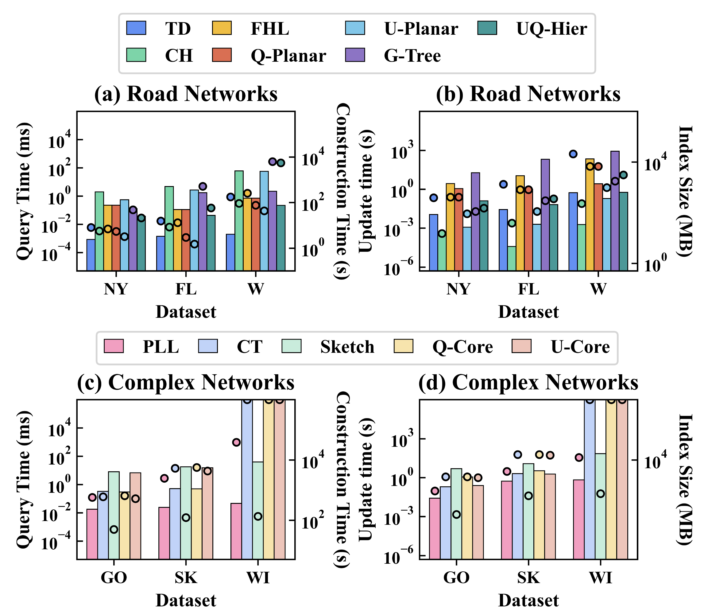
Figure 8: Shortest Path Index Comparison. (Bar: Query and Update Time; Ball: Construction Time and Index Size)

TABLE IV: Partition Strategy on CSP

	Pre-B		Post-B		No Partition Label		Search
	NY	COL	NY	COL	NY	COL	NY	COL
Construct (s)	25614	11378	194	983	1357	2022	-	-
Index (MB)	2483	14248	2483	14248	36450	103870	-	-
Query (ms)	0.001	0.002	0.001	0.002	0.0001	0.00007	1.1895	11.69

Exp 4: Influence on Complicated Path Problems (CSP). To better demonstrate the power of our partition strategies, we conduct experiments of 2-dimensional constrained shortest paths by optimizing FHL [16]. Apart from NY, we also test on Colorado (COL) network with 435,666 vertices and 1,057,0666 edges. As shown in Table IV, the post-boundary strategy is the fastest to construct and has the smallest label size. Although no partition label is the fastest in query, it is slow to construct and has huge index sizes. More importantly, it fails to construct on higher dimensional CSP scenarios [31]. As for the Pre-Boundary, it suffers from the slow boundary pair skyline path search while Post-Boundary solves it.

VI Related Work

We categorize the existing methods based on our scheme: 1) Pre-Boundary+Search/All-Pair+Hierarchy/Planar: These methods (HiTi [42], Graph Separators, Customizable Route Planning [28] [71], ParDiSP [98, 22]) pre-compute the shortest distance between boundaries (some hierarchically) to guide the search. In a broad sense, Arc-flag [23] and SHARC [24] also belong to this category. G-tree [43, 45] uses dynamic programming to compute the distance between layer’s all-pair information to replace searching, and it is widely used in kNN [44], ride-sharing [99], time-dependent routing [100], and machine learning-based path finding [101]. They are slow to construct due to Pre-B and slower to query to direct search; 2) Pre-Boundary+Search/PLL+Planar: COLA [15] builds the labels for the skyline shortest path on the overlay graph to answer the constrained shortest path query. This structure’s construction suffers from Pre-B and query suffers from searching; 3) Pre-Boundary+TD/TD+Planar: FHL [16, 31, 17] partition builds the TD both within and between partitions for multi-dimensional skyline paths. As validated in Exp 4, our Post-B can speedup Pre-B’s construction dramatically; 4) Pre-Boundary+PLL/ PLL+Planar: T2Hop [13, 14] utilizes two layers of PLL to reduce the complexity of long range time-dependent paths, and this structure’s performance is limited by PLL; 5) No-Boundary+ PLL/TD+Core: Core-Tree [6, 79] is the baseline and we have discussed it; 6) Pre-Boundary+Search/All-Pair/PLL+Sketch: This category works on huge graphs where index is nearly impossible so only a small number of landmarks are selected to either help prune the search [84, 29, 30] or approximate result [92, 94].

VII Conclusions

In this work, we decouple the partitioned shortest path indexes and propose a universal scheme with three dimensions: partitioned index strategy, path index, and partition structure. For partitioned index strategies, we propose two new strategies and pruned-boundary optimization for better index construction and update performance. For partition structure, we propose a new path-oriented classification and identify the factors influencing the PSP index performance. We also provide index maintenance solutions for classic PSP indexes. To demonstrate the usefulness of this scheme, we further recouple these dimensions and propose five new indexes that are either more efficient in query or update than the current state-of-the-arts.

References

- [1] H. Bast, D. Delling, A. Goldberg, M. Müller-Hannemann, T. Pajor, P. Sanders, D. Wagner, and R. F. Werneck, “Route planning in transportation networks,” in Algorithm engineering. Springer, 2016, pp. 19–80.
- [2] S. Boccaletti, V. Latora, Y. Moreno, M. Chavez, and D.-U. Hwang, “Complex networks: Structure and dynamics,” Physics reports, vol. 424, no. 4-5, pp. 175–308, 2006.
- [3] E. D. Kolaczyk, D. B. Chua, and M. Barthélemy, “Group betweenness and co-betweenness: Inter-related notions of coalition centrality,” Social Networks, vol. 31, no. 3, pp. 190–203, 2009.
- [4] T. Opsahl, F. Agneessens, and J. Skvoretz, “Node centrality in weighted networks: Generalizing degree and shortest paths,” Social networks, vol. 32, no. 3, pp. 245–251, 2010.
- [5] B. Yao, F. Li, and X. Xiao, “Secure nearest neighbor revisited,” in 2013 IEEE 29th international conference on data engineering (ICDE). IEEE, 2013, pp. 733–744.
- [6] W. Li, M. Qiao, L. Qin, Y. Zhang, L. Chang, and X. Lin, “Scaling up distance labeling on graphs with core-periphery properties,” in Proceedings of the 2020 ACM SIGMOD International Conference on Management of Data, 2020, pp. 1367–1381.
- [7] W. Li, M. Qiao, L. Qin, Y. Zhang, L. Chang, and X. Lin, “Scaling distance labeling on small-world networks,” in Proceedings of the 2019 International Conference on Management of Data, 2019, pp. 1060–1077.
- [8] M. Zhang, L. Li, and X. Zhou, “An experimental evaluation and guideline for path finding in weighted dynamic network,” Proceedings of the VLDB Endowment, vol. 14, no. 11, pp. 2127–2140, 2021.
- [9] M. Zhang, L. Li, W. Hua, R. Mao, P. Chao, and X. Zhou, “Dynamic hub labeling for road networks,” in 2021 IEEE 37th International Conference on Data Engineering (ICDE). IEEE, 2021, pp. 336–347.
- [10] M. Zhang, L. Li, W. Hua, and X. Zhou, “Efficient 2-hop labeling maintenance in dynamic small-world networks,” in 2021 IEEE 37th International Conference on Data Engineering (ICDE). IEEE, 2021, pp. 133–144.
- [11] M. Zhang, L. Li, G. Trajcevski, A. Zufle, and X. Zhou, “Parallel hub labeling maintenance with high efficiency in dynamic small-world networks,” IEEE Transactions on Knowledge and Data Engineering, 2023.
- [12] E. Cohen, E. Halperin, H. Kaplan, and U. Zwick, “Reachability and distance queries via 2-hop labels,” SIAM Journal on Computing, vol. 32, no. 5, pp. 1338–1355, 2003.
- [13] L. Li, S. Wang, and X. Zhou, “Time-dependent hop labeling on road network,” in 2019 IEEE 35th International Conference on Data Engineering (ICDE). IEEE, 2019, pp. 902–913.
- [14] L. Li, S. Wang, and X. Zhou, “Fastest path query answering using time-dependent hop-labeling in road network,” IEEE Transactions on Knowledge and Data Engineering, 2020.
- [15] S. Wang, X. Xiao, Y. Yang, and W. Lin, “Effective indexing for approximate constrained shortest path queries on large road networks,” Proceedings of the VLDB Endowment, vol. 10, no. 2, pp. 61–72, 2016.
- [16] Z. Liu, L. Li, M. Zhang, W. Hua, P. Chao, and X. Zhou, “Efficient constrained shortest path query answering with forest hop labeling,” in 2021 IEEE 37th International Conference on Data Engineering (ICDE). IEEE, 2021, pp. 1763–1774.
- [17] Z. Liu, L. Li, M. Zhang, W. Hua, and X. Zhou, “Fhl-cube: Multi-constraint shortest path querying with flexible combination of constraints,” Proceedings of the VLDB Endowment, vol. 15, 2022.
- [18] E. W. Dijkstra, “A note on two problems in connexion with graphs,” Numerische mathematik, vol. 1, no. 1, pp. 269–271, 1959.
- [19] P. E. Hart, N. J. Nilsson, and B. Raphael, “A formal basis for the heuristic determination of minimum cost paths,” IEEE transactions on Systems Science and Cybernetics, vol. 4, no. 2, pp. 100–107, 1968.
- [20] L. Li, M. Zhang, W. Hua, and X. Zhou, “Fast query decomposition for batch shortest path processing in road networks,” in 2020 IEEE 36th International Conference on Data Engineering (ICDE). IEEE, 2020, pp. 1189–1200.
- [21] M. Zhang, L. Li, W. Hua, and X. Zhou, “Stream processing of shortest path query in dynamic road networks,” IEEE Transactions on Knowledge and Data Engineering, 2020.
- [22] T. Chondrogiannis and J. Gamper, “Pardisp: A partition-based framework for distance and shortest path queries on road networks,” in 2016 17th IEEE International Conference on Mobile Data Management (MDM), vol. 1. IEEE, 2016, pp. 242–251.
- [23] R. H. Möhring, H. Schilling, B. Schütz, D. Wagner, and T. Willhalm, “Partitioning graphs to speedup dijkstra’s algorithm,” Journal of Experimental Algorithmics (JEA), vol. 11, pp. 2–8, 2007.
- [24] R. Bauer and D. Delling, “Sharc: Fast and robust unidirectional routing,” Journal of Experimental Algorithmics (JEA), vol. 14, pp. 2–4, 2010.
- [25] R. Geisberger, P. Sanders, D. Schultes, and D. Delling, “Contraction hierarchies: Faster and simpler hierarchical routing in road networks,” in International workshop on experimental and efficient algorithms. Springer, 2008, pp. 319–333.
- [26] T. Akiba, Y. Iwata, and Y. Yoshida, “Fast exact shortest-path distance queries on large networks by pruned landmark labeling,” in Proceedings of the 2013 ACM SIGMOD International Conference on Management of Data, 2013, pp. 349–360.
- [27] D. Ouyang, L. Qin, L. Chang, X. Lin, Y. Zhang, and Q. Zhu, “When hierarchy meets 2-hop-labeling: Efficient shortest distance queries on road networks,” in Proceedings of the 2018 International Conference on Management of Data, 2018, pp. 709–724.
- [28] D. Delling, A. V. Goldberg, T. Pajor, and R. F. Werneck, “Customizable route planning in road networks,” Transportation Science, vol. 51, no. 2, pp. 566–591, 2017.
- [29] Y. Wang, Q. Wang, H. Koehler, and Y. Lin, “Query-by-sketch: Scaling shortest path graph queries on very large networks,” in Proceedings of the 2021 International Conference on Management of Data, 2021, pp. 1946–1958.
- [30] M. Farhan, Q. Wang, and H. Koehler, “Batchhl: Answering distance queries on batch-dynamic networks at scale,” arXiv preprint arXiv:2204.11012, 2022.
- [31] Z. Liu, L. Li, M. Zhang, W. Hua, and X. Zhou, “Multi-constraint shortest path using forest hop labeling,” The VLDB Journal, pp. 1–27, 2022.
- [32] A. Pacaci and M. T. Özsu, “Experimental analysis of streaming algorithms for graph partitioning,” in Proceedings of the 2019 International Conference on Management of Data, 2019, pp. 1375–1392.
- [33] M. Holtgrewe, P. Sanders, and C. Schulz, “Engineering a scalable high quality graph partitioner,” in 2010 IEEE International Symposium on Parallel & Distributed Processing (IPDPS), 2010, pp. 1–12.
- [34] P. Sanders and C. Schulz, “Engineering multilevel graph partitioning algorithms,” in European Symposium on Algorithms. Springer, 2011, pp. 469–480.
- [35] D. Delling, A. V. Goldberg, I. Razenshteyn, and R. F. Werneck, “Graph partitioning with natural cuts,” in 2011 IEEE International Parallel Distributed Processing Symposium, 2011, pp. 1135–1146.
- [36] L. R. Ford and D. R. Fulkerson, “Maximal flow through a network,” Canadian journal of Mathematics, vol. 8, pp. 399–404, 1956.
- [37] S. T. Barnard and H. D. Simon, “Fast multilevel implementation of recursive spectral bisection for partitioning unstructured problems,” Concurrency: Practice and experience, vol. 6, no. 2, pp. 101–117, 1994.
- [38] B. Hendrickson and R. Leland, “A multilevel algorithm for partitioning graphs,” in Proceedings of the 1995 ACM/IEEE Conference on Supercomputing, 1995, pp. 28––es.
- [39] F. Pellegrini and J. Roman, “Scotch: A software package for static mapping by dual recursive bipartitioning of process and architecture graphs,” in International Conference on High-Performance Computing and Networking. Springer, 1996, pp. 493–498.
- [40] G. Karypis and V. Kumar, “A fast and high quality multilevel scheme for partitioning irregular graphs,” SIAM JOURNAL ON SCIENTIFIC COMPUTING, vol. 20, no. 1, pp. 359–392, 1998.
- [41] S. Jung and S. Pramanik, “Hiti graph model of topographical road maps in navigation systems,” in Proceedings of the Twelfth International Conference on Data Engineering. IEEE, 1996, pp. 76–84.
- [42] S. Jung and S. Pramanik, “An efficient path computation model for hierarchically structured topographical road maps,” IEEE Transactions on Knowledge and Data Engineering, vol. 14, no. 5, pp. 1029–1046, 2002.
- [43] R. Zhong, G. Li, K.-L. Tan, and L. Zhou, “G-tree: An efficient index for knn search on road networks,” in Proceedings of the 22nd ACM international conference on Information and Knowledge Management, 2013, pp. 39–48.
- [44] R. Zhong, G. Li, K.-L. Tan, L. Zhou, and Z. Gong, “G-tree: An efficient and scalable index for spatial search on road networks,” IEEE Transactions on Knowledge and Data Engineering, vol. 27, no. 8, pp. 2175–2189, 2015.
- [45] Z. Li, L. Chen, and Y. Wang, “G*-tree: An efficient spatial index on road networks,” in 2019 IEEE 35th International Conference on Data Engineering (ICDE). IEEE, 2019, pp. 268–279.
- [46] A. Pothen, H. D. Simon, and K.-P. Liou, “Partitioning sparse matrices with eigenvectors of graphs,” SIAM Journal on Matrix Analysis and Applications, vol. 11, no. 3, pp. 430–452, 1990.
- [47] T. Goehring and Y. Saad, “Heuristic algorithms for automatic graph partitioning,” Citeseer, Tech. Rep., 1994.
- [48] A. Buluç, H. Meyerhenke, I. Safro, P. Sanders, and C. Schulz, “Recent advances in graph partitioning,” Algorithm engineering, pp. 117–158, 2016.
- [49] R. Diekmann, R. Preis, F. Schlimbach, and C. Walshaw, “Shape-optimized mesh partitioning and load balancing for parallel adaptive fem,” Parallel Computing, vol. 26, no. 12, pp. 1555–1581, 2000.
- [50] S. Schamberger, “On partitioning fem graphs using diffusion,” in 18th International Parallel and Distributed Processing Symposium, 2004. Proceedings. IEEE, 2004, p. 277.
- [51] H. Meyerhenke, B. Monien, and S. Schamberger, “Accelerating shape optimizing load balancing for parallel fem simulations by algebraic multigrid,” in Proceedings 20th IEEE International Parallel & Distributed Processing Symposium. IEEE, 2006, pp. 10–pp.
- [52] M. J. Berger and S. H. Bokhari, “A partitioning strategy for nonuniform problems on multiprocessors,” IEEE Transactions on Computers, vol. C-36, no. 5, pp. 570–580, 1987.
- [53] H. D. Simon, “Partitioning of unstructured problems for parallel processing,” Computing systems in engineering, vol. 2, no. 2-3, pp. 135–148, 1991.
- [54] J. R. Gilbert, G. L. Miller, and S.-H. Teng, “Geometric mesh partitioning: Implementation and experiments,” SIAM Journal on Scientific Computing, vol. 19, no. 6, pp. 2091–2110, 1998.
- [55] Y.-W. Huang, N. Jing, and E. A. Rundensteiner, “Effective graph clustering for path queries in digital map databases,” in Proceedings of the fifth international conference on Information and knowledge management, 1996, pp. 215–222.
- [56] K. Schloegel, G. Karypis, and V. Kumar, “Graph partitioning for high performance scientific simulations,” 2000.
- [57] H. Saran and V. V. Vazirani, “Finding k cuts within twice the optimal,” SIAM Journal on Computing, vol. 24, no. 1, pp. 101–108, 1995.
- [58] N. Guttmann-Beck and R. Hassin, “Approximation algorithms for minimum k-cut,” Algorithmica, vol. 27, no. 2, pp. 198–207, 2000.
- [59] O. Goldschmidt and D. S. Hochbaum, “A polynomial algorithm for the k-cut problem for fixed k,” Mathematics of Operations Research, vol. 19, no. 1, pp. 24–37, 1994.
- [60] D. R. Karger and C. Stein, “A new approach to the minimum cut problem,” Journal of the ACM (JACM), vol. 43, no. 4, pp. 601–640, 1996.
- [61] M. Thorup, “Minimum k-way cuts via deterministic greedy tree packing,” in Proceedings of the fortieth annual ACM symposium on Theory of computing, 2008, pp. 159–166.
- [62] B. W. Kernighan and S. Lin, “An efficient heuristic procedure for partitioning graphs,” The Bell System Technical Journal, vol. 49, no. 2, pp. 291–307, 1970.
- [63] C. Fiduccia and R. Mattheyses, “A linear-time heuristic for improving network partitions,” in Proceedings of the 19th Design Automation Conference, 1982, pp. 175–181.
- [64] J. E. Gonzalez, Y. Low, H. Gu, D. Bickson, and C. Guestrin, “PowerGraph: Distributed Graph-Parallel computation on natural graphs,” in 10th USENIX symposium on operating systems design and implementation (OSDI 12), 2012, pp. 17–30.
- [65] J. E. Gonzalez, R. S. Xin, A. Dave, D. Crankshaw, M. J. Franklin, and I. Stoica, “GraphX: Graph processing in a distributed dataflow framework,” in 11th USENIX symposium on operating systems design and implementation (OSDI 14), 2014, pp. 599–613.
- [66] A. Roy, L. Bindschaedler, J. Malicevic, and W. Zwaenepoel, “Chaos: Scale-out graph processing from secondary storage,” in Proceedings of the 25th Symposium on Operating Systems Principles, 2015, pp. 410–424.
- [67] F. Petroni, L. Querzoni, K. Daudjee, S. Kamali, and G. Iacoboni, “Hdrf: Stream-based partitioning for power-law graphs,” in Proceedings of the 24th ACM international on conference on information and knowledge management, 2015, pp. 243–252.
- [68] D. Kong, X. Xie, and Z. Zhang, “Clustering-based partitioning for large web graphs,” arXiv preprint arXiv:2201.00472, 2022.
- [69] C. Zhang, F. Wei, Q. Liu, Z. G. Tang, and Z. Li, “Graph edge partitioning via neighborhood heuristic,” in Proceedings of the 23rd ACM SIGKDD International Conference on Knowledge Discovery and Data Mining, 2017, pp. 605–614.
- [70] M. Hanai, T. Suzumura, W. J. Tan, E. Liu, G. Theodoropoulos, and W. Cai, “Distributed edge partitioning for trillion-edge graphs,” Proceedings of the VLDB Endowment, vol. 12, no. 13.
- [71] M. Holzer, F. Schulz, and D. Wagner, “Engineering multilevel overlay graphs for shortest-path queries,” Journal of Experimental Algorithmics (JEA), vol. 13, pp. 2–5, 2009.
- [72] K. C. Lee, W.-C. Lee, and B. Zheng, “Fast object search on road networks,” in Proceedings of the 12th International Conference on Extending Database Technology: Advances in Database Technology, 2009, pp. 1018–1029.
- [73] K. C. Lee, W.-C. Lee, B. Zheng, and Y. Tian, “Road: A new spatial object search framework for road networks,” IEEE transactions on knowledge and data engineering, vol. 24, no. 3, pp. 547–560, 2010.
- [74] R. Mayer and H.-A. Jacobsen, “Hybrid edge partitioner: Partitioning large power-law graphs under memory constraints,” in Proceedings of the 2021 International Conference on Management of Data, 2021, pp. 1289–1302.
- [75] R. Geisberger, P. Sanders, D. Schultes, and C. Vetter, “Exact routing in large road networks using contraction hierarchies,” Transportation Science, vol. 46, no. 3, pp. 388–404, 2012.
- [76] D. Ouyang, L. Yuan, L. Qin, L. Chang, Y. Zhang, and X. Lin, “Efficient shortest path index maintenance on dynamic road networks with theoretical guarantees,” Proceedings of the VLDB Endowment, vol. 13, no. 5, pp. 602–615, 2020.
- [77] V. J. Wei, R. C.-W. Wong, and C. Long, “Architecture-intact oracle for fastest path and time queries on dynamic spatial networks,” in Proceedings of the 2020 ACM SIGMOD International Conference on Management of Data, 2020, pp. 1841–1856.
- [78] R. Jin, Z. Peng, W. Wu, F. Dragan, G. Agrawal, and B. Ren, “Parallelizing pruned landmark labeling: dealing with dependencies in graph algorithms,” in Proceedings of the 34th ACM International Conference on Supercomputing, 2020, pp. 1–13.
- [79] B. Zheng, J. Wan, Y. Gao, Y. Ma, K. Huang, X. Z. Zhou, and C. S. Jensen, “Workload-aware shortest path distance querying in road networks,” in 2022 IEEE 38th International Conference on Data Engineering (ICDE). IEEE, 2022.
- [80] L. Chang, J. X. Yu, L. Qin, H. Cheng, and M. Qiao, “The exact distance to destination in undirected world,” The VLDB Journal, vol. 21, no. 6, pp. 869–888, 2012.
- [81] F. Wei, “Tedi: efficient shortest path query answering on graphs,” in Graph Data Management: Techniques and Applications. IGI global, 2012, pp. 214–238.
- [82] Z. Chen, A. W.-C. Fu, M. Jiang, E. Lo, and P. Zhang, “P2h: Efficient distance querying on road networks by projected vertex separators,” in Proceedings of the 2021 International Conference on Management of Data, 2021, pp. 313–325.
- [83] T. Maehara, T. Akiba, Y. Iwata, and K.-i. Kawarabayashi, “Computing personalized pagerank quickly by exploiting graph structures,” Proceedings of the VLDB Endowment, vol. 7, no. 12, pp. 1023–1034, 2014.
- [84] A. Das Sarma, S. Gollapudi, M. Najork, and R. Panigrahy, “A sketch-based distance oracle for web-scale graphs,” in Proceedings of the third ACM international conference on Web search and data mining, 2010, pp. 401–410.
- [85] S. P. Borgatti and M. G. Everett, “Models of core/periphery structures,” Social networks, vol. 21, no. 4, pp. 375–395, 2000.
- [86] M. P. Rombach, M. A. Porter, J. H. Fowler, and P. J. Mucha, “Core-periphery structure in networks,” SIAM Journal on Applied mathematics, vol. 74, no. 1, pp. 167–190, 2014.
- [87] A. Elliott, A. Chiu, M. Bazzi, G. Reinert, and M. Cucuringu, “Core–periphery structure in directed networks,” Proceedings of the Royal Society A, vol. 476, no. 2241, p. 20190783, 2020.
- [88] T. Maehara, T. Akiba, Y. Iwata, and K.-i. Kawarabayashi, “Computing personalized pagerank quickly by exploiting graph structures,” Proceedings of the VLDB Endowment, vol. 7, no. 12, pp. 1023–1034, 2014.
- [89] N. Robertson and P. D. Seymour, “Graph minors. iii. planar tree-width,” Journal of Combinatorial Theory, Series B, vol. 36, no. 1, pp. 49–64, 1984.
- [90] J. Xu, F. Jiao, and B. Berger, “A tree-decomposition approach to protein structure prediction,” in 2005 IEEE Computational Systems Bioinformatics Conference (CSB’05). IEEE, 2005, pp. 247–256.
- [91] M. Potamias, F. Bonchi, C. Castillo, and A. Gionis, “Fast shortest path distance estimation in large networks,” in Proceedings of the 18th ACM conference on Information and knowledge management, 2009, pp. 867–876.
- [92] A. Gubichev, S. Bedathur, S. Seufert, and G. Weikum, “Fast and accurate estimation of shortest paths in large graphs,” in Proceedings of the 19th ACM international conference on Information and knowledge management, 2010, pp. 499–508.
- [93] K. Tretyakov, A. Armas-Cervantes, L. García-Bañuelos, J. Vilo, and M. Dumas, “Fast fully dynamic landmark-based estimation of shortest path distances in very large graphs,” in Proceedings of the 20th ACM international conference on Information and knowledge management, 2011, pp. 1785–1794.
- [94] M. Qiao, H. Cheng, L. Chang, and J. X. Yu, “Approximate shortest distance computing: A query-dependent local landmark scheme,” IEEE Transactions on Knowledge and Data Engineering, vol. 26, no. 1, pp. 55–68, 2012.
- [95] Z. Qi, Y. Xiao, B. Shao, and H. Wang, “Toward a distance oracle for billion-node graphs,” Proceedings of the VLDB Endowment, vol. 7, no. 1, pp. 61–72, 2013.
- [96] M. Farhan, Q. Wang, Y. Lin, and B. Mckay, “A highly scalable labelling approach for exact distance queries in complex networks,” EDBT, 2018.
- [97] H.-P. Kriegel, P. Kröger, M. Renz, and T. Schmidt, “Hierarchical graph embedding for efficient query processing in very large traffic networks,” in International Conference on Scientific and Statistical Database Management. Springer, 2008, pp. 150–167.
- [98] T. Chondrogiannis and J. Gamper, “Exploring graph partitioning for shortest path queries on road networks,” in 26th GI-Workshop Grundlagen von Datenbanken: GvDB’14, 2014, pp. 71–76.
- [99] N. Ta, G. Li, T. Zhao, J. Feng, H. Ma, and Z. Gong, “An efficient ride-sharing framework for maximizing shared route,” IEEE Transactions on Knowledge and Data Engineering, vol. 30, no. 2, pp. 219–233, 2017.
- [100] Y. Wang, G. Li, and N. Tang, “Querying shortest paths on time dependent road networks,” Proceedings of the VLDB Endowment, vol. 12, no. 11, pp. 1249–1261, 2019.
- [101] S. Huang, Y. Wang, T. Zhao, and G. Li, “A learning-based method for computing shortest path distances on road networks,” in 2021 IEEE 37th International Conference on Data Engineering (ICDE). IEEE, 2021, pp. 360–371.