XIMAGENET-12: An Explainable AI Benchmark Dataset for Model Robustness Evaluation

Abstract

The lack of standardized robustness metrics and the widespread reliance on numerous unrelated benchmark datasets for testing have created a gap between academically validated robust models and their often problematic practical adoption. To address this, we introduce XIMAGENET-12, an explainable benchmark dataset with over 200K images and 15,600 manual semantic annotations. Covering 12 categories from ImageNet to represent objects commonly encountered in practical life and simulating six diverse scenarios, including overexposure, blurring, color changing, etc., we further propose a novel robustness criterion that extends beyond model generation ability assessment. This benchmark dataset, along with related code, is available at https://sites.google.com/view/ximagenet-12/home. Researchers and practitioners can leverage this resource to evaluate the robustness of their visual models under challenging conditions and ultimately benefit the demands of practical computer vision systems.

1 Introduction

Visual models have widely been utilized in the industrial sector, especially OEMs (Original Equipment Manufacturers) specializing in large-scale computer vision applications for defect detection[1], image enhancement [2], quality control[3], and predictive maintenance topics [4, 5]. Those models often touted as highly effective in academic settings that excel on large benchmark datasets, tend to exhibit surprising shortcomings when deployed in real-world scenarios [4, 6, 7]. Issues such as sensitivity to changes in lighting conditions, background interference, shifts in object positions, and the presence of previously unseen noise or artificial camera disturbances in the background are common challenges that supposedly stable models, as claimed in academic papers, often fail to address adequately [3, 5].

Researchers from academia often lack a readily available and interpretable dataset to explore the specifics of how AI utilizes information for content understanding and which cues it is really sensitive to. Creating such a dataset typically requires extensive manual labeling efforts and resources. Therefore, we decided to use the well-known ImageNet dataset [8] as a foundation for our work, as it serves as a cornerstone in the field of convolutional neural networks (CNNs) and is extensively used to evaluate visual models. However, ImageNet [8] is primarily a classification dataset, meaning it provides only category labels for each class and sometimes includes some images that do not belong to their designated categories. Recent advancements in Explainable machine learning [9] have led to various improvements in this direction, such as the IOG dataset [10], which starts with ImageNet and filters 1,000 images per class using neural networks to create virtual labels. There’s also the ImageNet-9 dataset [11], which selects nine classes and explores the impact of backgrounds on foreground objects, using neural networks to assign labels for each class and experimenting with background replacements. Some approaches [12] even utilize graph neural networks (GNNs) to generate semantic labels for ImageNet. While these efforts have been inspiring, they still suffer from significant drawbacks. Using neural networks to generate pseudo labels [13, 14, 15, 16] can introduce significant inaccuracies (see Fig. 6. Furthermore, datasets like ImageNet-9 [11] do not deeply investigate how backgrounds influence model performance; they merely suggest that backgrounds are not always noise and can sometimes be helpful, touching upon the finding that more robust models tend to rely less on backgrounds without quantitative comparison.

Hence, our team embarked long journey involving over 20 contributors to the annotation process and designed our dataset to cover 12 major categories, including objects that fly, swim, and are commonly found in everyday life, as well as some intricate multi-background objects. In total, we meticulously annotated over 12,000 images at the pixel level and conducted further research into scenarios like background replacement, complete background removal for enhanced validation, background blurring, foreground blurring, and color changes to simulate object shifts caused by camera vibrations in industrial production processes. Additionally, we explored artificially rendered backgrounds and backgrounds generated by the Stable Diffusion model [17] to examine the model’s sensitivity to different image variations.

The creative highlight of our work lies in the in-depth exploration of the state-of-the-art (SOTA) models, including Transformer-based models and segmentation models as well to analyze their sensitivity to image backgrounds. We have delved into defining model robustness, as existing robustness tests [18, 19] typically involve stacking massive amounts of irrelevant data that often differ significantly from the objects’ backgrounds encountered in industrial settings. Strong performance on benchmark datasets does not necessarily translate to high accuracy in real-world industrial projects [20]. Furthermore, model robustness should encompass the ability to recognize foreground objects accurately even in the presence of various new variables introduced by background interference. Therefore, our work combines dataset creation, quantitative model analysis, and the innovative proposal of a robustness comparison formula, allowing for a comparative evaluation of model robustness and providing guidance for practical engineering model usage. Our main contributions can be summarized as follows:

• We annotate and GenAI generate a dataset for the explainable AI domain and Gen-AI domain, which possesses various annotation categories, relatively high image information quality, and public availability.

• We propose the model robustness score formal schema based our dataset for a better selection of models for industry applications.

• We quantitatively analyses and benchmark SOTA object detection, classification, and segmentation models using our dataset encompasses both CNN- and Transformer-based architectures, aimed at validating the models’ robustness while prioritizing explainable AI principles.

2 Dataset creation procedure:

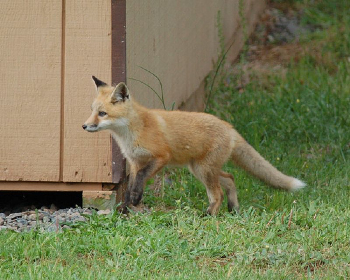
original image

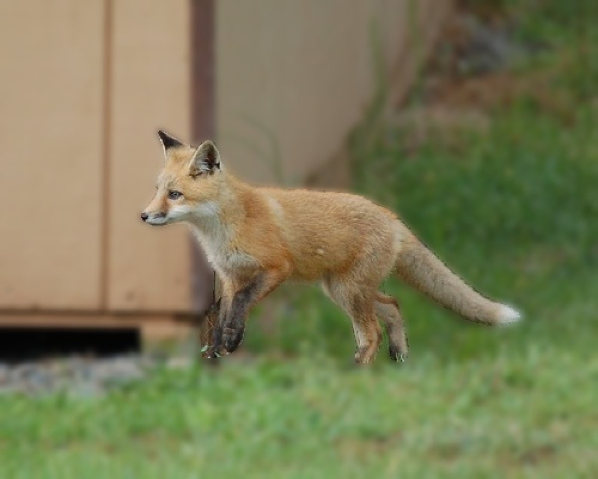
Blurred background

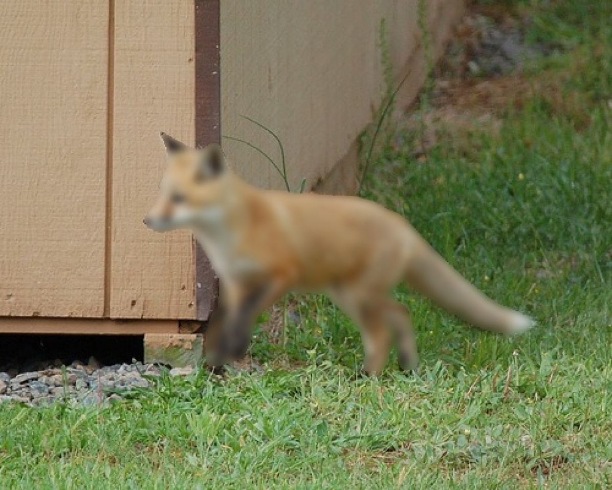
Blurred foreground

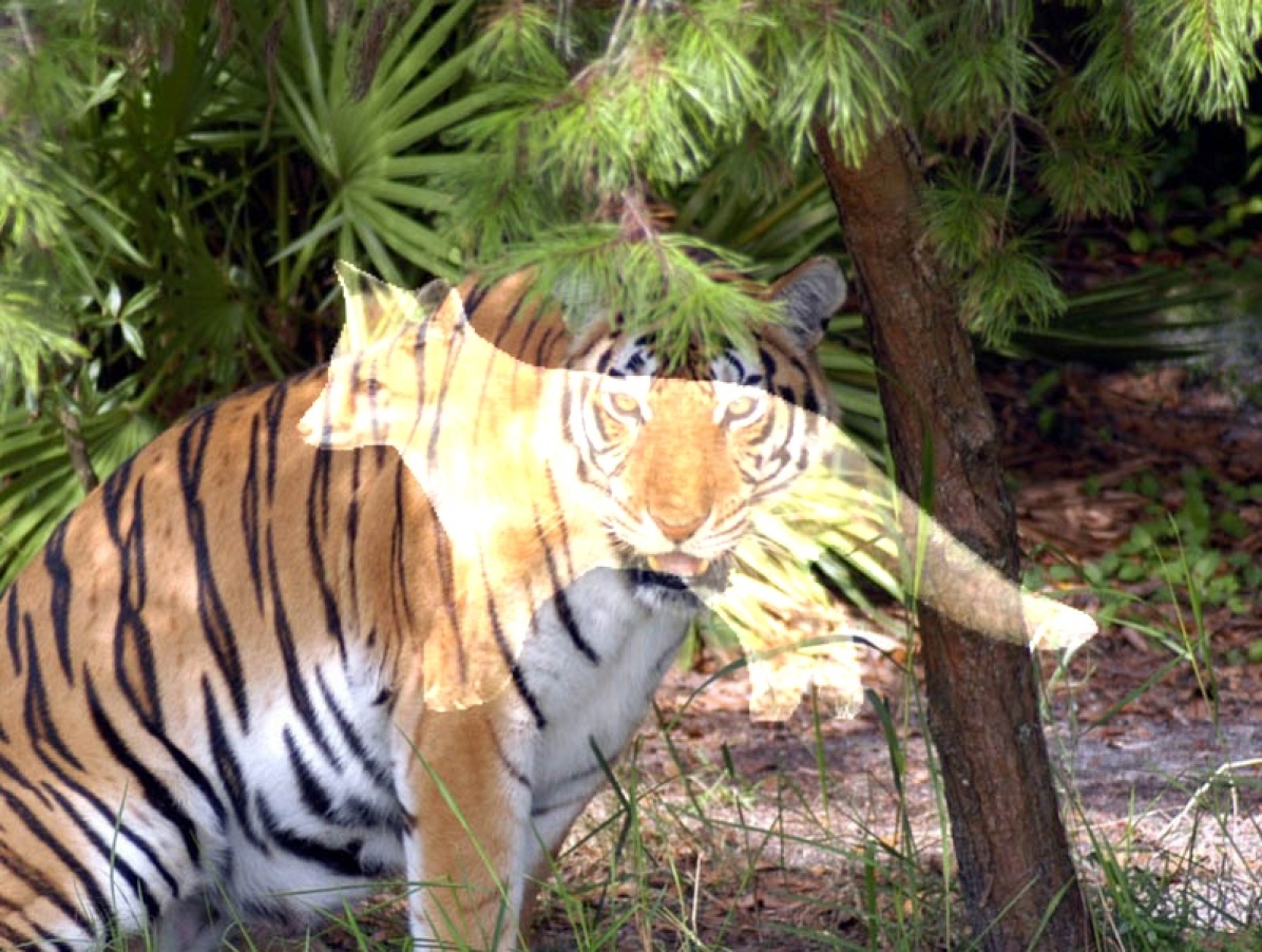
Random generated

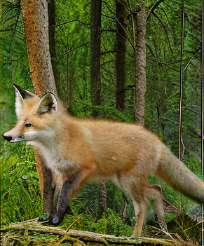
AI generated

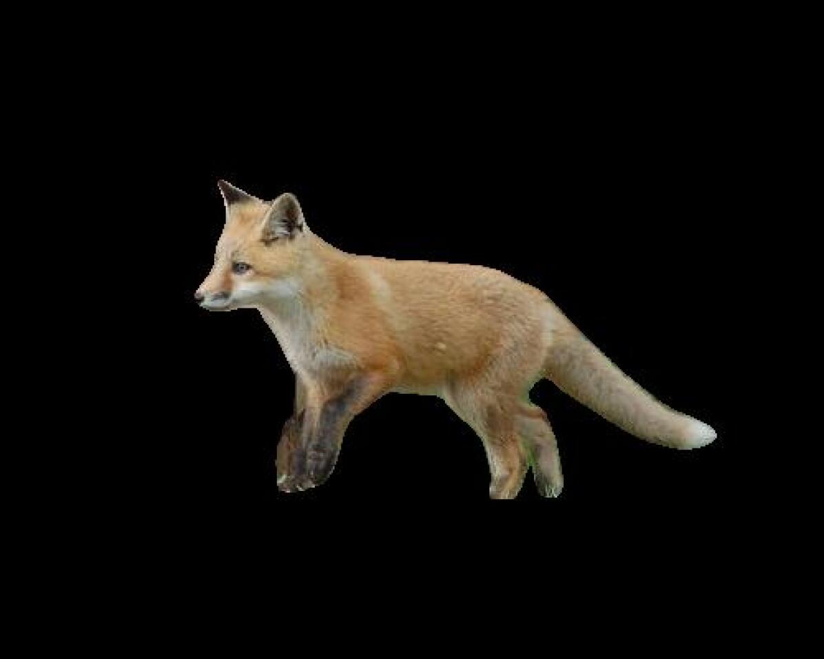
Segmented image

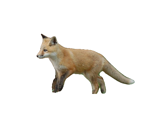
Transparent image

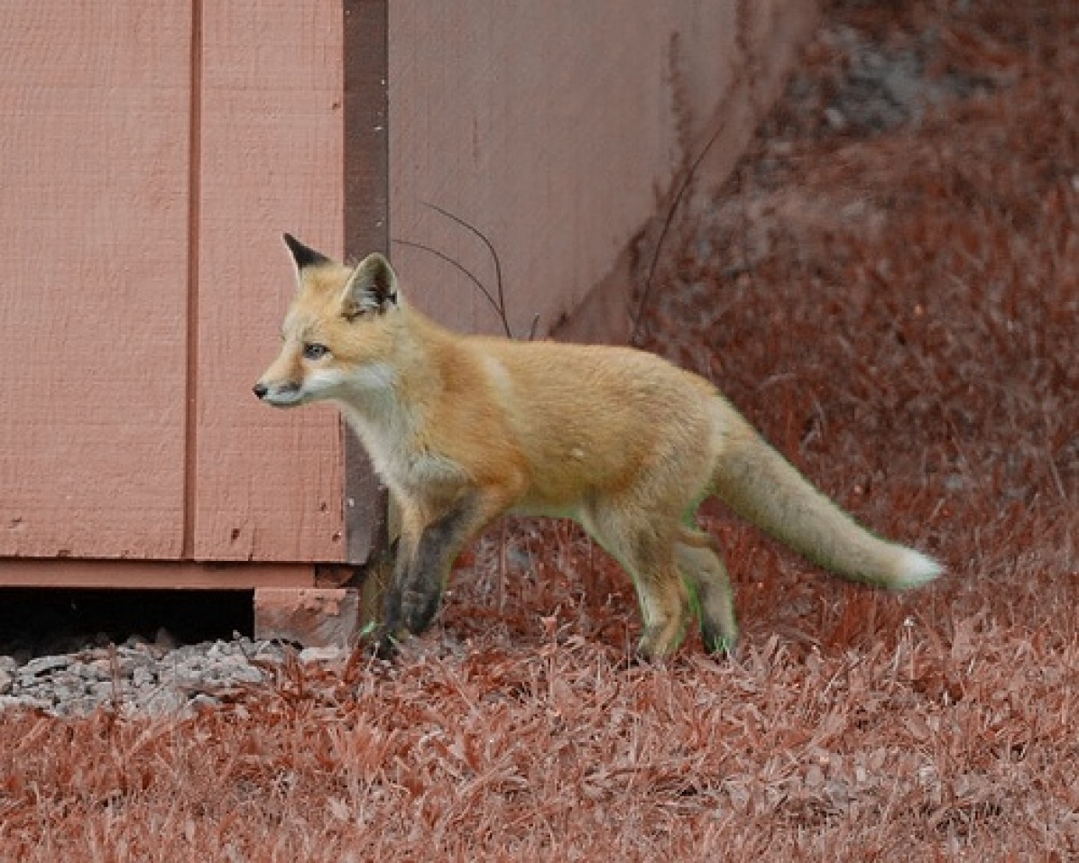
Color R-channel

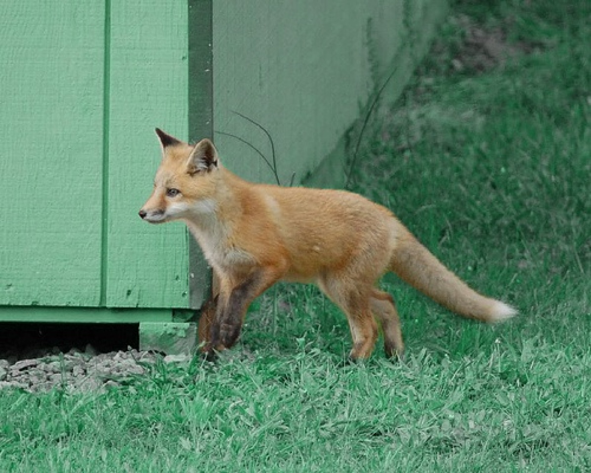
Color G-channel

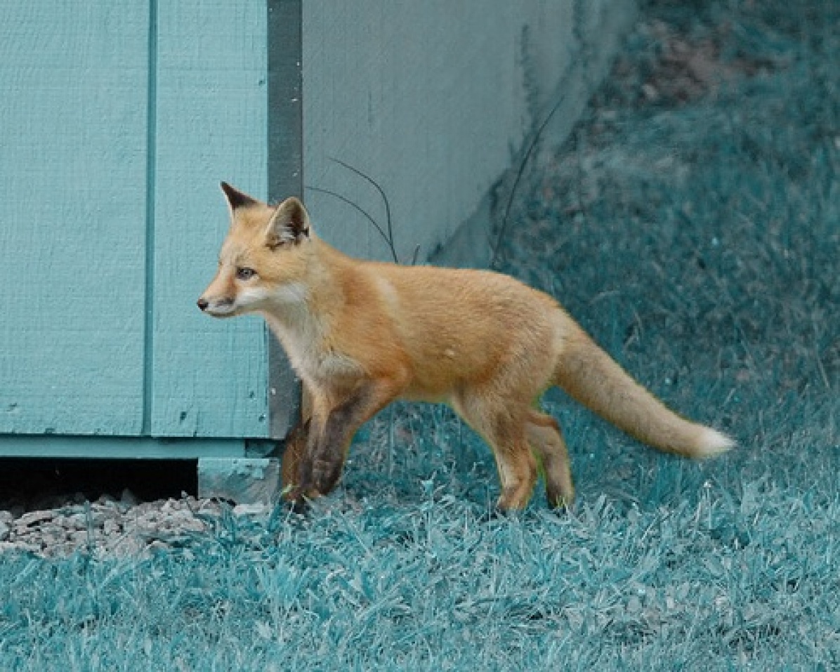
Color B-channel

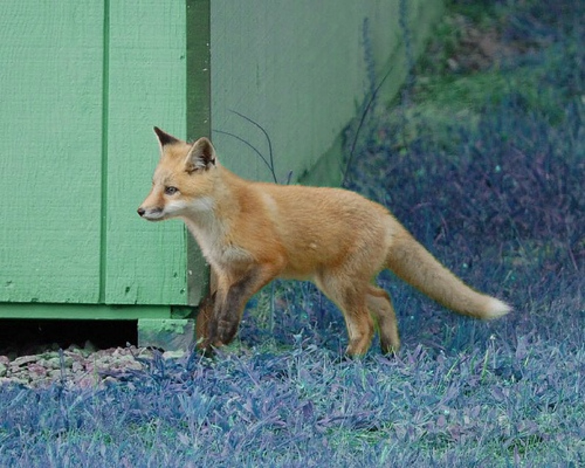
Color rainbow

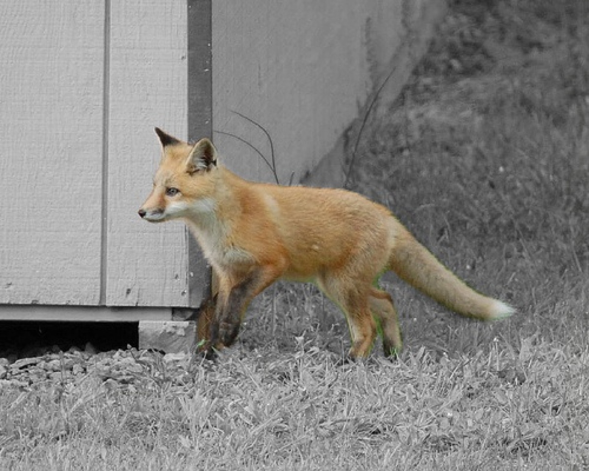
Color grayscale

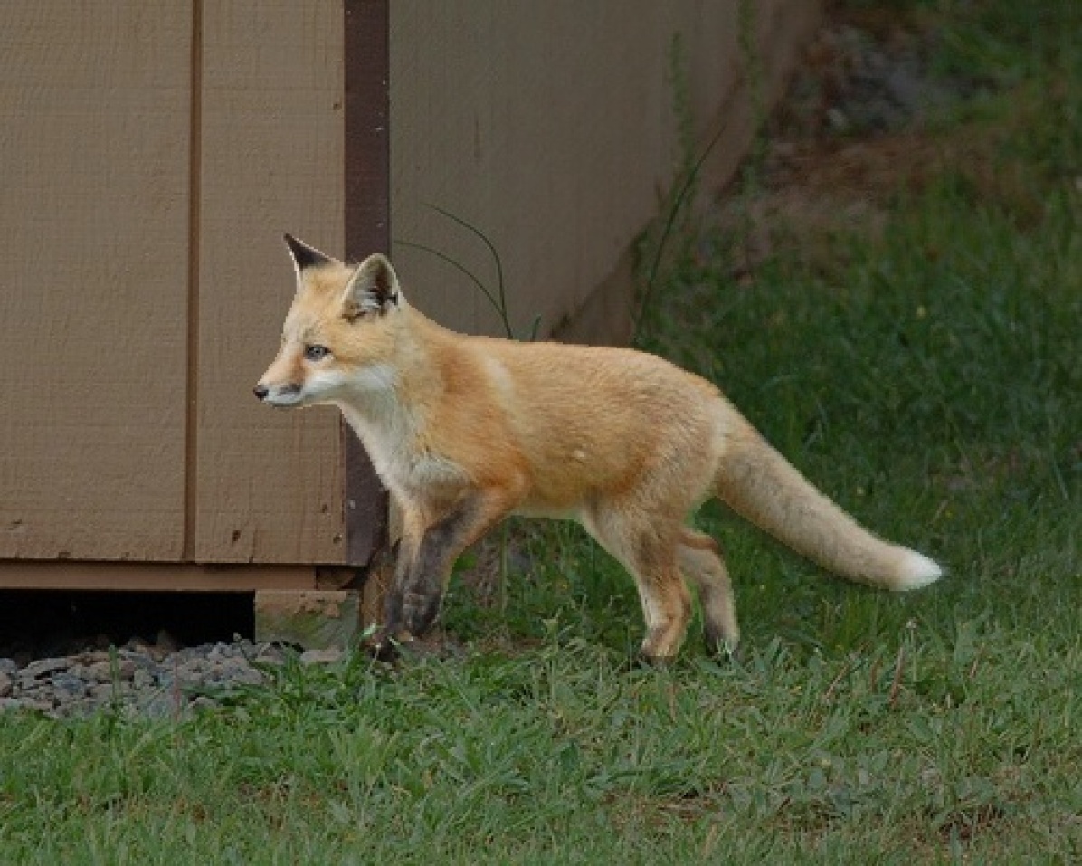
Bright background

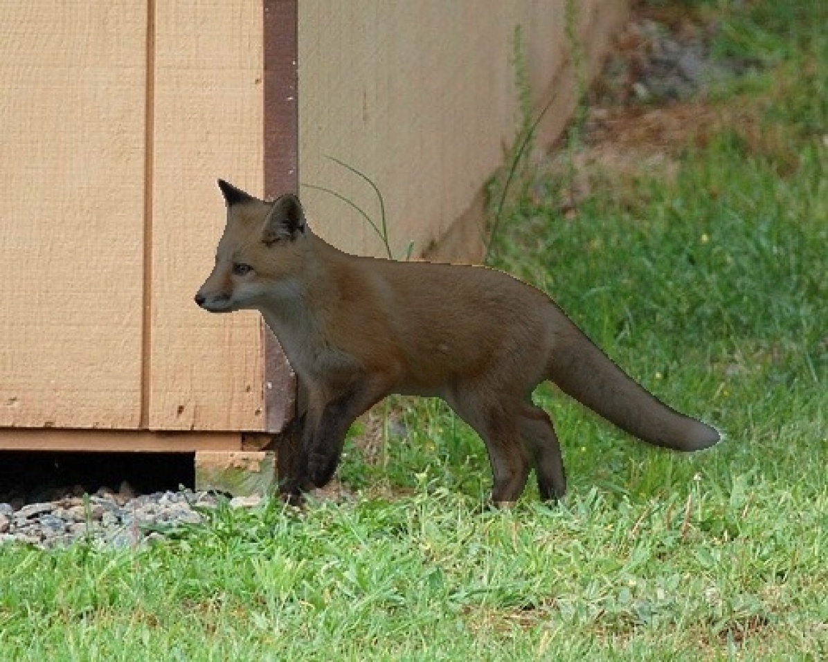
Bright foreground

Figure 1: XIMAGENET-12 sample for 6 scenarios: Blur, Random generated background, AI-generated background, Segmentated, Transparent and Color images. Over 200K Images in total.

In this section, we will introduce our dataset from three aspects: (1) the process of image capturing, (2) the overall properties of our dataset, and (3) the composition of our dataset.

2.1 Data Collection

12 categories are selected from the ImageNet dataset as the fundamental image, which represents objects frequently encountered in everyday life. Then we synthesize 6 scenarios (refer to Fig.1) to comprehensively evaluate model robustness. These scenarios include blurred images, colored images, segmented images, transparent images, images with randomly generated backgrounds, and images with AI-generated backgrounds.

Colored images: In this scenario, we enrich the diversity of dataset by generating images from grayscale, single-channel (R, G, B), rainbow images, and different brightness of both background and foreground. The process of grayscale and single-channel is to keep the object in a color image unchanged while altering the background to grayscale or individual RGB channels. The function addWeighted in OpenCV is used to apply Unsharp Masking (USM) to enhance brightness and sharpness. The rainbow image is generated by converting the image to HSV color space and changing the hue for the background. Color images can simulate the changes in lighting and color conditions in the real world. Keeping the object of interest unchanged allows for better analysis of the object’s characteristics and reduces distractions from the background.

Blurred images: By combining with mask information, we propose two ways of blurring images: blurring the image background and blurring the foreground object. The function GaussianBlur in OpenCV is used to apply the blur properties to the image. In real applications, blur often happens when a camera is small shifted, which leads to a loss of fine-grained details and compressed information. By weakening the background/foreground we have a preliminary understanding of the impact of background and foreground on model inference [21].

Segmented images: This scenario is composed of segmented objects only. To be specific, we create the new image with RGBA 4 channels, and the RGB channel pixel information will be unchanged for the foreground, and the alpha channel based on the binary mask. For example, if the pixel at (x, y) in the original image is (r, g, b), based on the binary mask, it will become (r, g, b, 255), if it is in the background then (0, 0, 0, 255). This scenario can enhance the interpretability of various computer vision tasks by highlighting objects of interest and separating them from the background [22].

Transparent images: There is a serious problem when using segmented images to generate AI background images, the Stable Diffusion XL model [23] will also take the alpha channel value into account [17], leading to lots of black spots surrounding the object. In order to overcome the problem, we create transparent images. Similar to the segmented scenario, we also create a new image with RGBA 4 channels, based on the binary mask, the background will be completely removed and the object will be kept the same. For example, if the pixel at (x, y) in the original image is (r,g,b), based on the binary mask, it will become (0, 0, 0, 0) if it is in the background, otherwise, it will be (r, g, b, 255).

Images with randomly generated backgrounds: In this scenario, images are generated with the photographer’s real image as a background and blended with the object from the original image. Specifically, When selecting background pictures, we deliberately choose pictures that are closely related to the natural environment. This scenario simulated the challenge of distorting the real environment. Because of addWeighted blending, resize, random Shuffle and position function, we can give different weights to different images, which can make the image transparent or translucent according to the weight added. As a result, the model becomes more robust and likely to generalize better to real-world scenarios where the background is unpredictable.

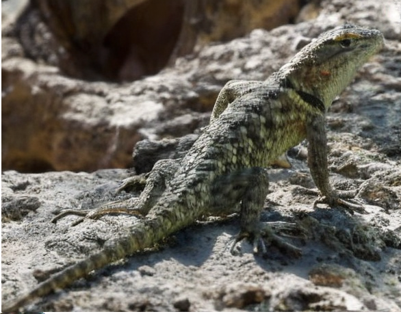
(a) Prompt: Generate high-definition pictures like those in the National Geographic magazine, keep the background unchanged.

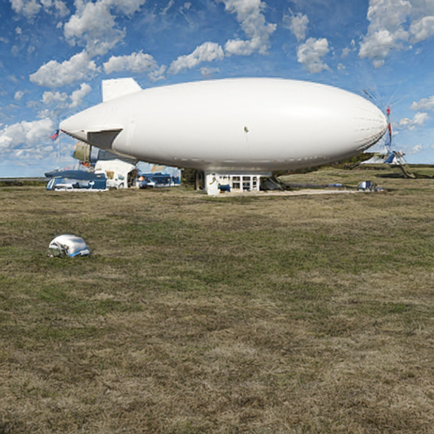
(b) Prompt: Generate a realistic blue sky, and clouds background and please do not change the foreground airship object.

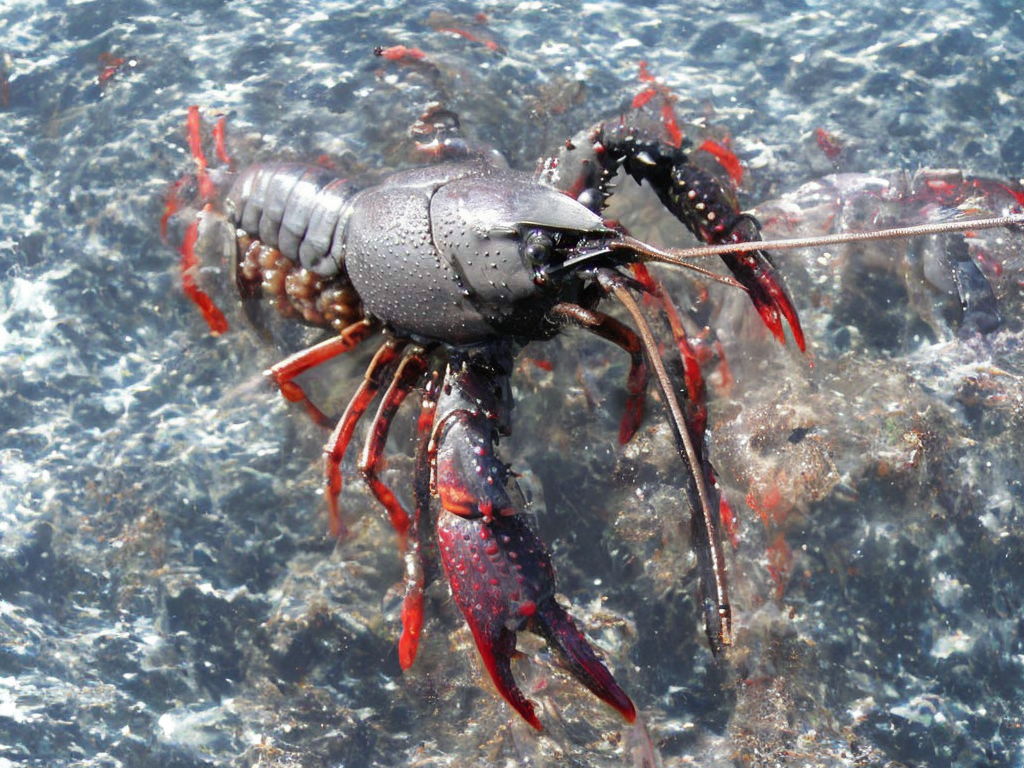
(c) Prompt: Generate high resolution images in sea water

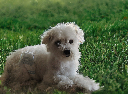
(d) Prompt: Generate a picture with a foreground and the green grass in the background, similar to the official HD picture released by the state.

(e) Prompt: Generate high-resolution pictures like fox in the lawn, National Geographic, keep the background and foreground more simple and real.

(f) Prompt: Generate a simple image more realistic in the style of ocean magazine.

(g) Prompt: Generate an image with the car in the background and similar to the HD image published by the state.

(h) Prompt: Generate high-resolution pictures like those in National Financial Magazine, and keep the background and foreground consistent and the environment more real!

(i) Prompt: Please generate high-resolution pictures like those in the National Music Magazine and keep the background unchanged.

(j) Prompt: Generate high-resolution pictures in the style of those in National Food Magazine, and keep the background and foreground consistent and the environment more real!

(k) Prompt: Generate high-definition pictures like those in the National Geographic magazine, keep the background unchanged.

(l) Prompt: Generate high-resolution pictures, such as National Marine Magazine’s oceans and whales, to keep the background real.

Figure 7: AI generated images with prompts.

Images with AI-generated backgrounds: Except randomly generating unrelated backgrounds, we also create a scenario where image backgrounds are generated by AI. Specifically, the backgrounds are created using Playground AI [24] by providing transparent images as input, following the Stable Diffusion XL model [23] for text-to-image generation with appropriate prompts. Different prompts are applied to different classes (See Fig.7), some very useful tips: Using keywords such as ‘National Geographic Magazine’ or ‘National Oceanic Magazine’ can increase the authenticity of the generated background; Adding specific and appropriate environmental information to the prompt can make the generated background and objects better integrated. By using a diffusion model and introducing unexpected or extreme background variations, we can assess whether the model is resilient against potential adversarial attacks involving background manipulation.

2.2 Dataset Properties

Aiming to show the properties of XIMAGENET-12 clearly, we illustrate the causality in the following perspectives:

Practicality: The 12 categories selected from ImageNet represent objects commonly encountered in practical life, and the scenarios we created accurately simulate problems that may be encountered in industry, such as brightness change, and background interference.

Scenarios: In addition to the fundamental images, XIMAGENET-12 is composed of 6 scenarios, which are colored images (gray, single-channel, rainbow, brightness change), blurred images (blurred background, blurred foreground), images with randomly generated backgrounds, images with AI-generated backgrounds, segmented images, and transparent images.

Foreground invariance: This invariance is relative to the variability of the background, through the whole XIMAGENET-12, the background is changed in each scenario, while most of the foreground object remains the same.

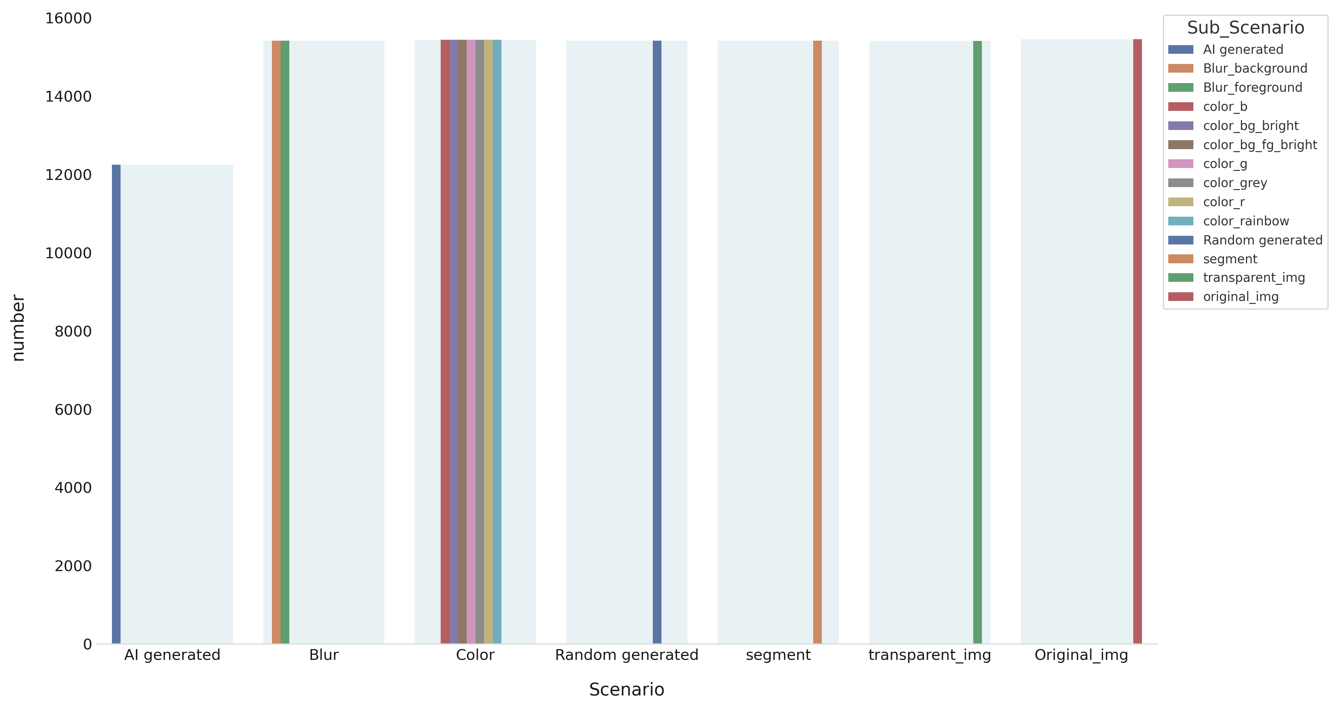
Figure 2: The scenario distribution of XIMAGENET-12.

2.3 Dataset Distribution

Fig.2 illustrates the distribution of our dataset across various scenarios, including fundamental images. We’ve curated 12 classes from ImageNet, each containing around 1,300 samples, resulting in a total selection of 15,450 images from ImageNet. As images from six scenarios are derived from fundamental images, each transformation within a scenario results in approximately 15,400 images. However, generating AI background images presented challenges, such as dealing with scenarios featuring multiple objects in a single image and the presence of small or incomplete objects. Nevertheless, through the collaborative efforts of our contributors, we successfully obtained 12,248 images for AI generated scenarios, with approximately 1,000 images for each class. In summary, XIMAGENET-12 includes 12 classes across six scenarios, encompassing a total of 212,787 images. We have also secured all intellectual property rights for these synthesized images.

3 experiment

3.1 Settings

We conducted benchmark tests on various SOTA object detection, classification, and segmentation models using XImageNet12 dataset. This encompassed a wide range of models from TensorFlow Keras, including the ResNet [25] series, MobileNet [26], EfficientNet [27] series, InceptionNet, DenseNet [28], and PyTorch framework models, including Transformer-based models like ViT [29]. In addition, we included nine models from the MMDetection framework [30], such as Deeplabv3plus R50-D8 [31] and Upernet models [32] with ViT-B16 and LN-MLN transformers.

To ensure the validity of our results, we meticulously reproduced all model accuracy claims as documented in official Keras library documentation (see Tab. 3 and Tab. 2). To mitigate random bias, we employed 12-fold cross-validation and reproduced the results over these folds.

We primarily conducted our experiments using TensorFlow and PyTorch, adhering to the standard hyperparameters provided in the official repositories. To quantitatively evaluate model robustness, we performed three distinct experiments: ’extra-scenarios’ (referred to as EX1), ’inter-scenarios’ (referred to as EX2), and ’AI-generated image segmentation’ (abbreviated as EX3 for simplicity on later sections of our paper). Each experiment involved multi-person verification to ensure reproducible results.

For EX1, namely extra-scenarios experiments, we used trained best weights from ImageNet original image and to test on our scenarios image to obtain the accuracy sensitivity for each scenario, because those scenarios were never learned by those visual models. For Tensorflow-based training, we adopted industry-recognized models such as ResNet-50 [25] and employed the SGD optimizer with (100 epochs) schedules, using a global batch size of 16 on a single T4 GPU, without data augmentation and input images had a resolution of 224×224 pixels. Transformer-based models, including ViT [29] models, utilized the Adam optimize under 0.0001 learning rate, with 200 epochs schedules and a global batch size of 16 distributed across 4 GPUs. Input images had a resolution of 224×224 pixels, with other settings mirroring those used in PyTorch-based experiments.

For EX2, namely inter-scenarios, we utilized representative models, including ResNet101 [25], MobileNetV3 [26], DenseNet121 [28] etc, alongside Transformer-based models like ViT [29]. Our goal was to assess model robustness explicitly for each subclass objects, such as instruments and animals, within the same scenarios. We conducted all 12-fold classifications within 6 scenarios. We also incorporated early stopping and multi-scale training, using standardized resizing input images to dimensions between 224 and 224 pixels. For Transformer-based models, settings remained consistent within inter-scenario experiments.

For EX3, namely segmentation experiments, we focused on evaluating the performance of top-performing models, such as Swin-Transformer [33], ViT series [29], PsPNet [34], FPN [35], UperNet [32] and DeepLabV3 [36] with ResNet50 [25] as the backbone on synthetically AI-generated background images and their accuracy in predicting masks for problematic pixels along edges and boundaries. Training occurred over 40,000 iterations, with a global batch size of 4 distributed across 2 GPUs. Train image comes from original ImageNet with crop size of 256×256 pixels, 2582 images, and testing on our XimageNet-12 background scenarios images, including 2,463 AI-generated background images.

All testing was performed using original resolution input images, without any augmentation or learned models applied. Later we performed all Multiple linear regression on collect test accuracy results on each scenarios or sub classes to quantitatively prove the hypothesise we made.

Table 1: Performance Evaluation of Multiple Linear Regression in Experiment 1: Modeling Scenarios. With ResNet50 model and original image as baseline intercept.

Variable	Estimate	Standard error	95% CI (asymptotic)	P value	P value summary
Intercept	0.8986	0.02238	0.8547 to 0.9426	$<0.0001$	****
Model Name[EfficientNetB0 [27] Best Weight]	-0.03444	0.01445	-0.06282 to -0.006065	0.0175	*
Model Name[EfficientNetB3 [27] Best Weight]	-0.04111	0.01445	-0.06949 to -0.01273	0.0046	**
Model Name[DenseNet121 [28] Best Weight]	0.01556	0.01445	-0.01282 to 0.04394	0.2821	ns
Model Name[MobileNetV2 [26] Best Weight]	0.005556	0.01445	-0.02282 to 0.03394	0.7007	ns
Image Scenario[blur_background]	-0.0425	0.01938	-0.08058 to -0.004424	0.0288	*
Image Scenario[blur_object]	-0.07	0.01938	-0.1081 to -0.03192	0.0003	***
Image Scenario[image_g]	-0.1257	0.01938	-0.1637 to -0.08759	$<0.0001$	****
Image Scenario[image_b]	-0.0985	0.01938	-0.1366 to -0.06042	$<0.0001$	****
Image Scenario[image_grey]	-0.06517	0.01938	-0.1032 to -0.02709	0.0008	***
Image Scenario[image_r]	-0.087	0.01938	-0.1251 to -0.04892	$<0.0001$	****
Image Scenario[Random Background with Real Environment]	-0.7078	0.01938	-0.7459 to -0.6698	$<0.0001$	****
Image Scenario[Segmented_image]	-0.3012	0.01938	-0.3392 to -0.2631	$<0.0001$	****
Image Class[1]	0.134	0.02238	0.09003 to 0.1780	$<0.0001$	****
Image Class[2]	-0.04867	0.02238	-0.09263 to -0.004701	0.0301	*
Image Class[3]	0.04	0.02238	-0.003966 to 0.08397	0.0745	ns
Image Class[4]	0.1004	0.02238	0.05648 to 0.1444	$<0.0001$	****
Image Class[5]	0.1333	0.02238	0.08937 to 0.1773	$<0.0001$	****
Image Class[6]	0.07667	0.02238	0.03270 to 0.1206	0.0007	***
Image Class[7]	0.01044	0.02238	-0.03352 to 0.05441	0.6409	ns
Image Class[8]	0.09067	0.02238	0.04670 to 0.1346	$<0.0001$	****
Image Class[9]	0.09933	0.02238	0.05537 to 0.1433	$<0.0001$	****
Image Class[10]	0.1651	0.02238	0.1211 to 0.2091	$<0.0001$	****
Image Class[11]	-0.02244	0.02238	-0.06641 to 0.02152	0.3164	ns

Table 2: EX1 and EX2 performance Comparison of SOTA Models on Different Test/Train Datasets.

Pretrained Dataset	Model Name	Parameters (M)	Test Dataset (Top-1 Acc.)
			Blur_bg	Blur_obj	Color_g	Color_b	Color_grey	Color_r	Rand_bg	Seg_img
ImageNet (Original images)	ResNet50 [25]	25.60	90.97%	88.17%	84.42%	86.98%	92.13%	89.03%	22.41%	68.55%
	VGG-16 [37]	138.4	89.92%	89.91%	78.64%	70.46%	81.48%	80.68%	24.58%	49.62%
	MobileNetV2 [26]	3.5	92.34%	88.52%	85.73%	88.67%	88.81%	89.33%	27.14%	66.43%
	EfficientNetB0 [27]	5.3	91.44%	90.86%	78.10%	82.45%	86.44%	83.65%	25.29%	53.56%
	EfficientNetB3 [27]	12.3	86.80%	84.53%	77.99%	81.22%	83.00%	83.85%	22.06%	69.67%
	DenseNet121 [28]	8.1	93.77%	88.92%	87.39%	87.33%	93.23%	88.21%	26.41%	69.67%
	ViT [29]	86.6	88.44%	90.77%	65.87%	62.82%	70.69%	66.53%	17.21%	49.01%
XImageNet-12 (*Scenarios)	ResNet50 [25]	25.60	83.52%	80.24%	83.61%	84.45%	84.71%	80.40%	53.91%	85.76%
	VGG-16 [37]	138.4	74.85%	71.54%	74.18%	76.26%	77.58%	69.91%	70.25%	73.27%
	AlexNet [38]	61.1	81.60%	79.95%	81.96%	81.89%	81.31%	78.07%	46.29%	82.00%
	MobileNetV3 [39]	3.50	67.36%	67.88%	72.04%	74.25%	69.48%	64.79%	43.33%	78.85%
	DenseNet121 [28]	8,1	90.79%	86.57%	88.92%	89.96%	90.44%	87.37%	69.58%	91.60%
	ViT [29]	86.56	71.51%	70.21%	74.77%	75.96%	75.80%	71.14%	38.01%	78.69%

3.2 Results And Finding: EX1

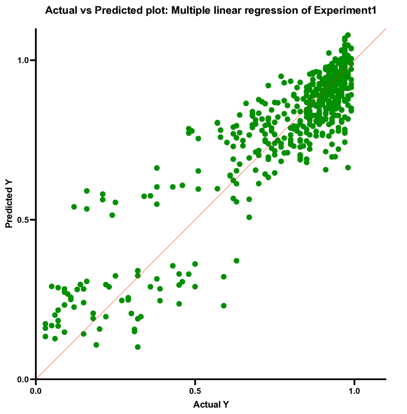
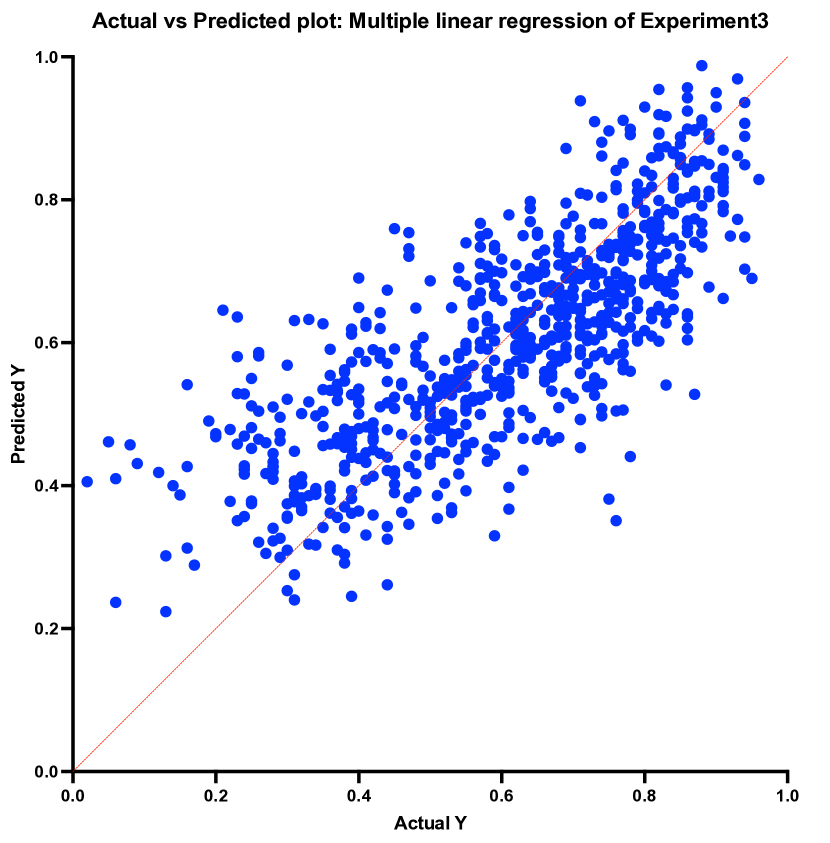
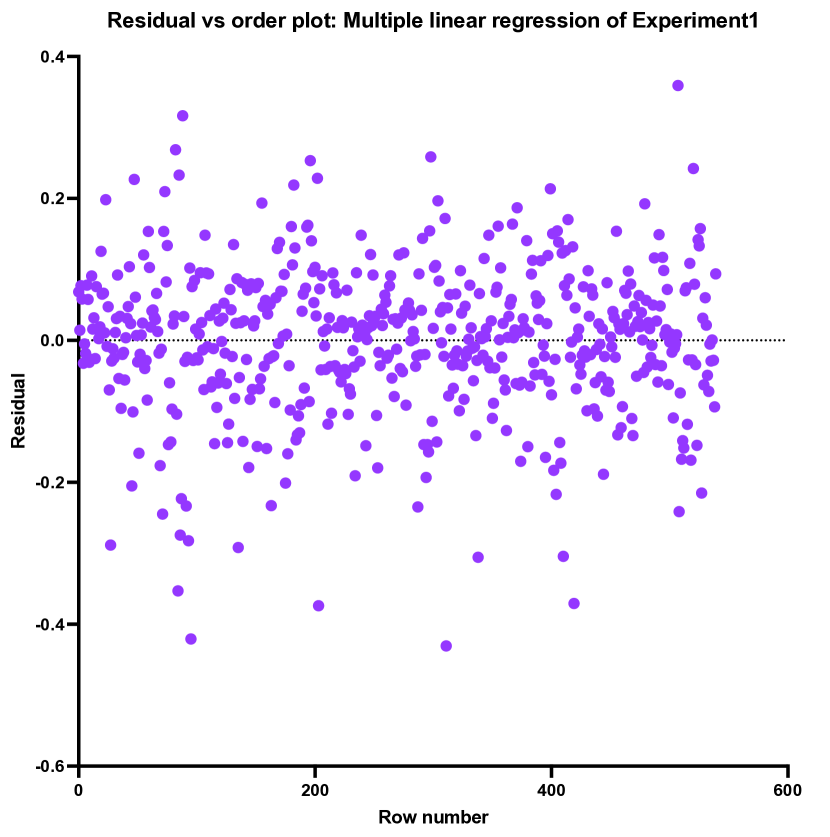
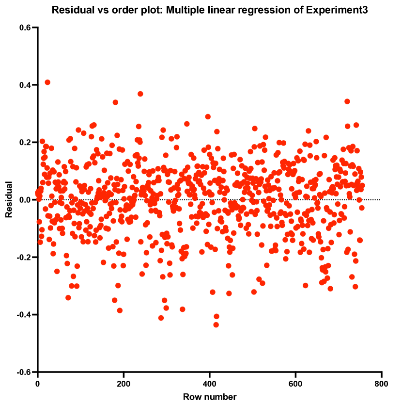
Figure 10: Multiple linear regression performance of Experiment 1 and Experiment 3.

Results on CNN-based methods. We conducted multiple linear regression analyses (Fig. 10) to examine our hypotheses using the accuracy drop data (Tab. 1, 5). This regression model aimed to predict ’Classification Accuracy’ based on three groups of predictor variables: ’Model Name,’ ’Image Scenarios,’ and ’Object Class.’ Our overall model yielded statistical significance with $F(23,516)=99.40$ and $P<0.0001$, indicating the relevance of at least one predictor variable in predicting the dependent variable. Specifically, ’Model Name’ exhibited statistical significance with $F(4,516)=6.125$ and $P<0.0001$. ’Image Scenarios’ also showed significance with $F(8,516)=257.2$ and $P<0.0001$. Lastly, ’Object Class’ demonstrated statistical significance with $F(11,516)=18.54$ and $P<0.0001$.

In our accuracy drop experiments, our experiments revealed a noticeable decline in accuracy, particularly when considering the accuracy density map Fig. 5 and variance Fig. 4. Notably, we observed that the presence of ’Random Background with Real Environment’ had the most substantial adverse impact on accuracy, resulting in a significant decrease of 0.7078. Furthermore, the ’Segmented Image’ scenario also exhibited a significant negative influence, leading to a decrease in accuracy by 0.3012 with a high level of statistical significance ($P<0.0001$). This observation reinforces the idea that models trained exclusively on backgrounds can significantly affect accuracy, highlighting the importance of background information in content reasoning. Our findings also support the hypothesis that more accurate models tend to be less reliant on background information. This is evident from the fact that the model with the highest top-1 accuracy during training exhibited less sensitivity to background scenarios [11].

Additionally, when considering specific model architectures, ’DenseNet121 [28] Best Weight’ demonstrated a small increase in accuracy by 0.015. Similarly, ’MobileNetV2 [26] Best Weight’ led to an accuracy increase of 0.005, which was less pronounced.

It is important to note that alterations to background color or image blurring had a negative impact on accuracy. However, this impact was less severe than the effect of introducing random backgrounds or complete background segmentation. Specifically, each of these modifications resulted in a noticeable difference of 0.1 to 0.2 percent, which remains statistically significant. Additionally, we found that ’Object Class 10’ and ’Object Class 5’ had the most positive impact on accuracy, leading to increases of 0.1651 and 0.1333, respectively. These effects were highly significant when compared to classes 6 and 7. This observation underscores the sensitivity of our explainable model to specific object classes, suggesting that the inherent attributes of objects play a significant role in content reasoning (see Tab.  2).

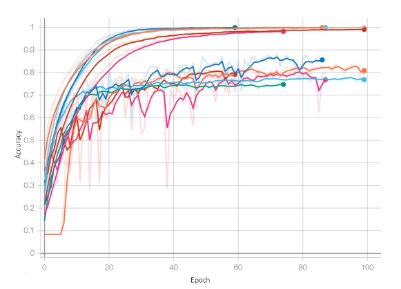
(a) Training accuracy for SOTA models for Experiment 1

(b) Training losses for SOTA models for Experiment 1

(c) Training details for SOTA models

Figure 3: Training details and loss plot for Experiment 1.

Top-1 Accuracy on EfficientNetB0

Top-1 Accuracy on EfficientNetB3

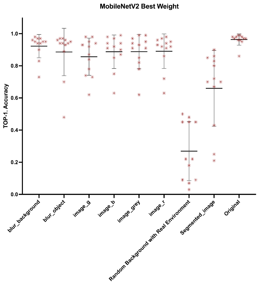
Top-1 Accuracy on MobileNetV2

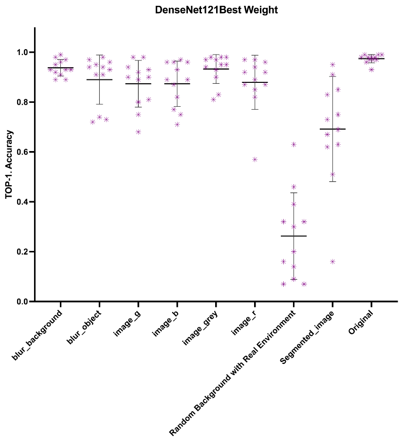
Top-1 Accuracy on DenseNet121

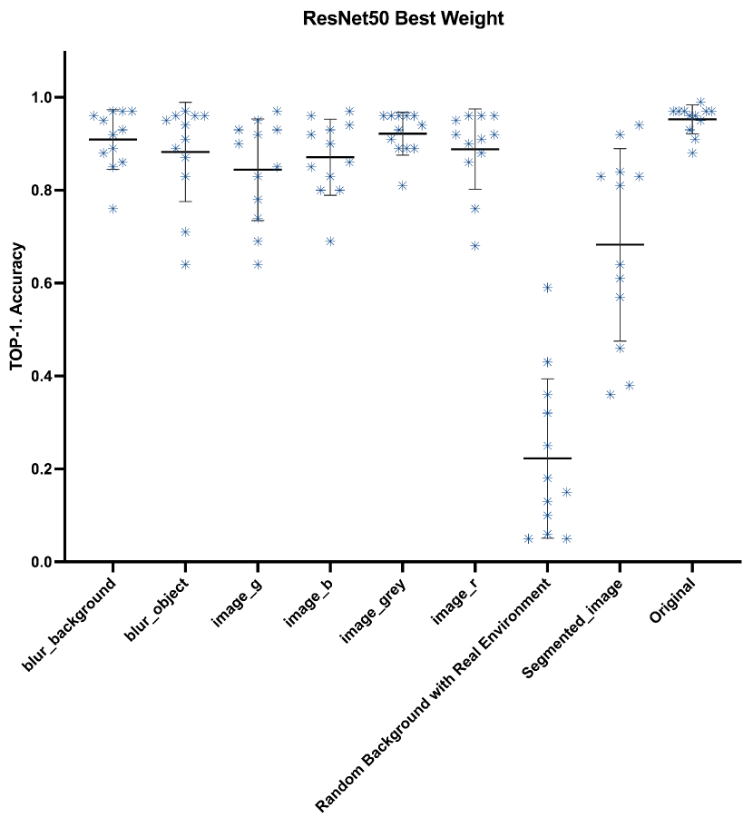
Top-1 Accuracy on ResNet50

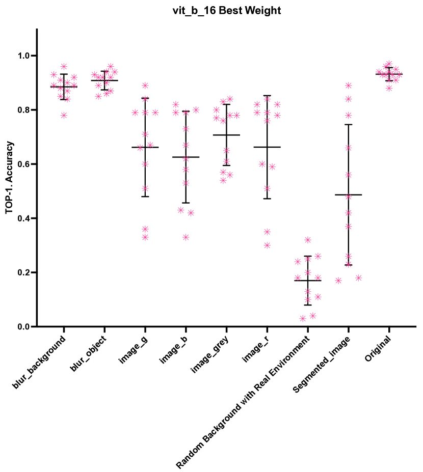
Top-1 Accuracy on ViT

Figure 4: TOP-1 Accuracy for SOTA models pre-trained on IMAGENET original images and tested on XIMAGENET-12.

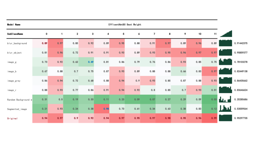
The EfficientNetB0 accuracy for each class

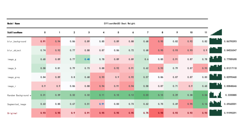
The EfficientNetB3 accuracy for each class

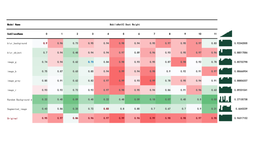
The MobileNetV2 accuracy for each class

The ViT accuracy for each class

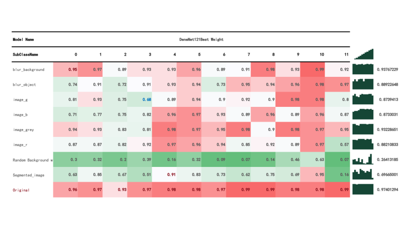
The DenseNet121 accuracy for each class

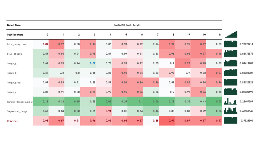
The ResNet50 accuracy for each class

Figure 5: The SOTA models accuracy density map for each class on Experiment 1.

Results on Transformer-based methods. We conducted an evaluation of the Vision Transformer (ViT) model [29] using the PyTorch framework on the XimageNet-12 dataset. Our results, presented in Tab. 2, showcase the model’s performance when pretrained on original images and tested on scenarios involving blurred backgrounds, with a mean Average Precision (mAP) of 88.43 for Blur Background and 90.76 for Blur Object images. Notably, ViT [29] demonstrates a substantial improvement in mAP, with a 26.4 increase when compared to Color Scenarios, for example, Image Green Channel (mAP 62.81)(see Tab. 2).

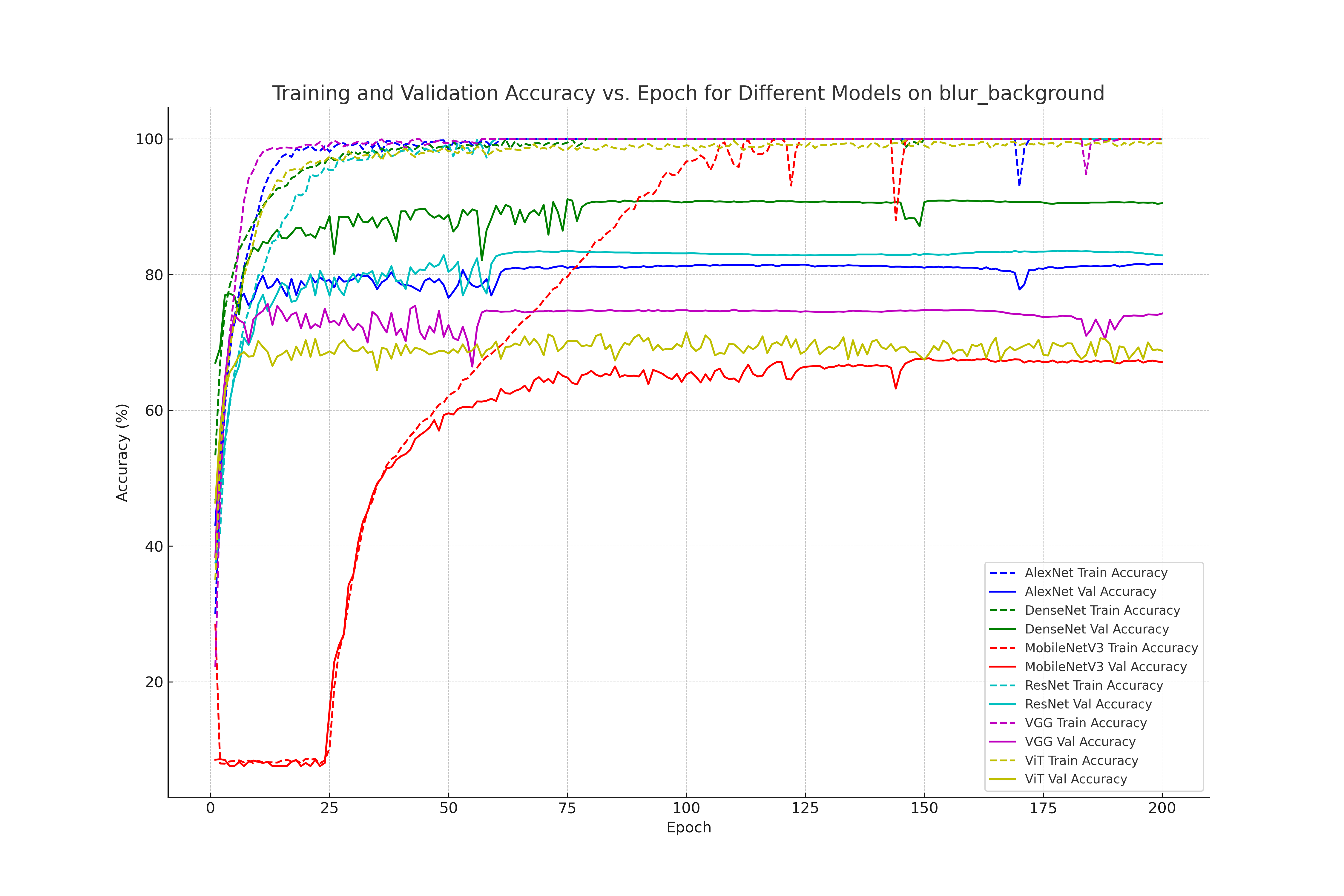
Top-1 training and validation accuracy on blurred background images

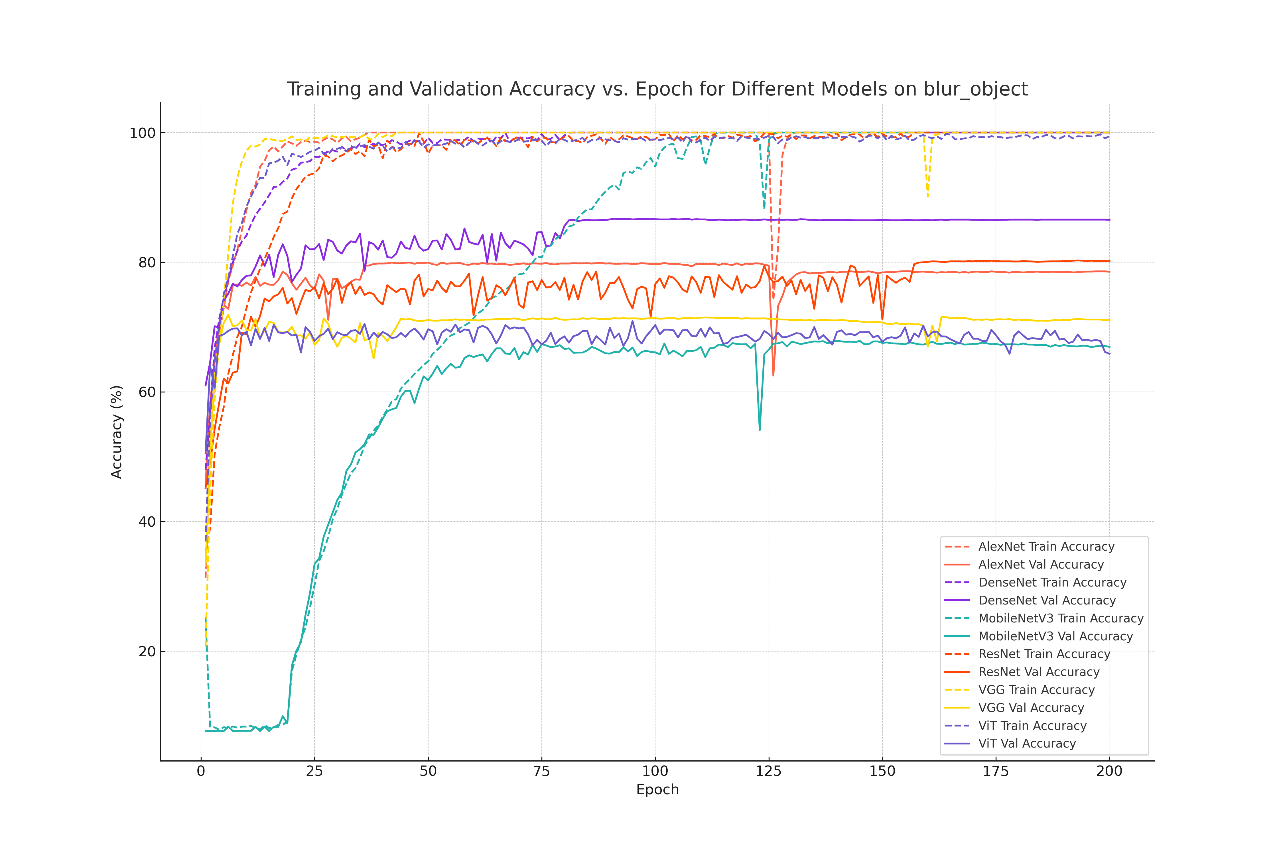
Top-1 training and validation accuracy on blurred object images

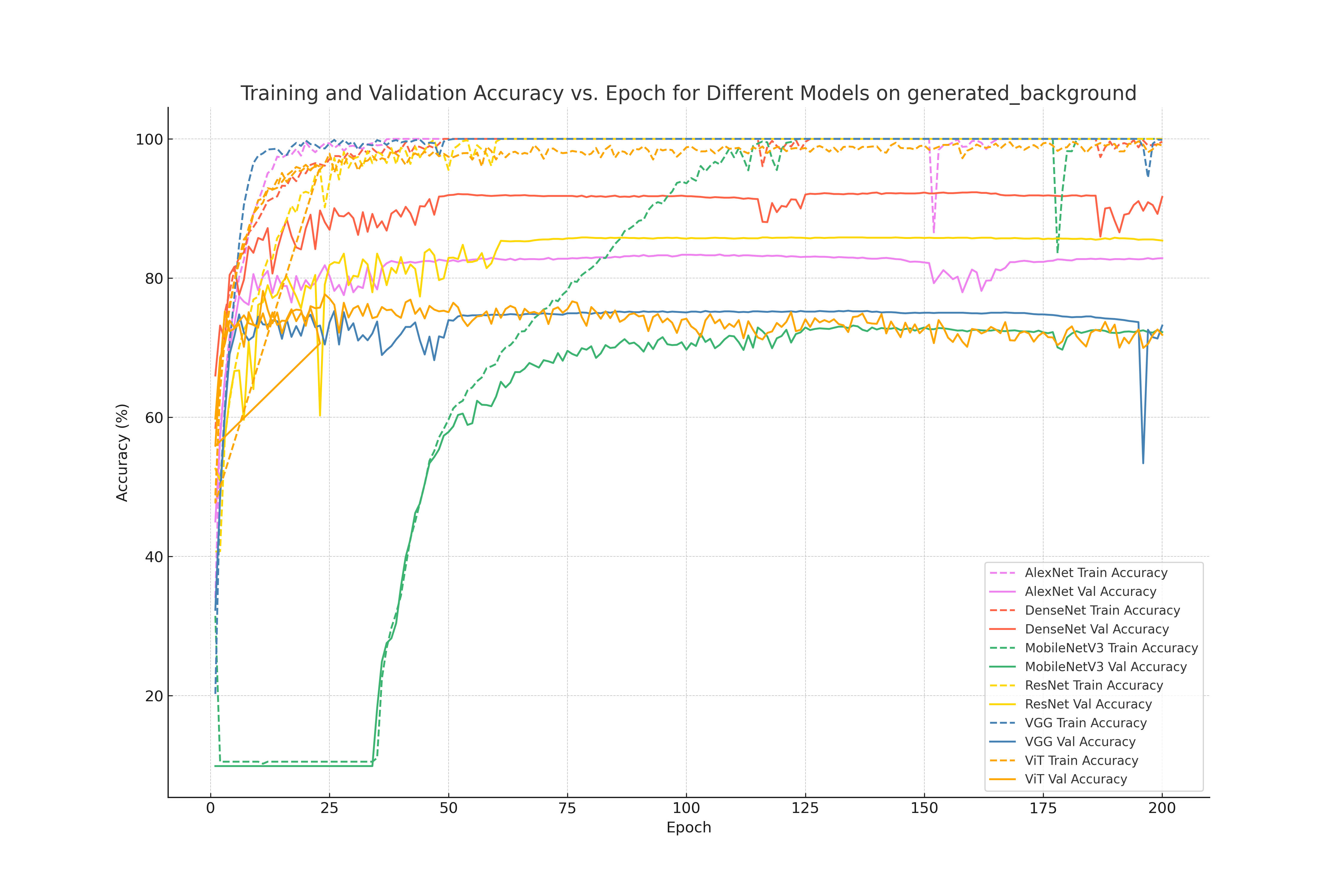
Top-1 training and validation accuracy on AI-generated background scenario

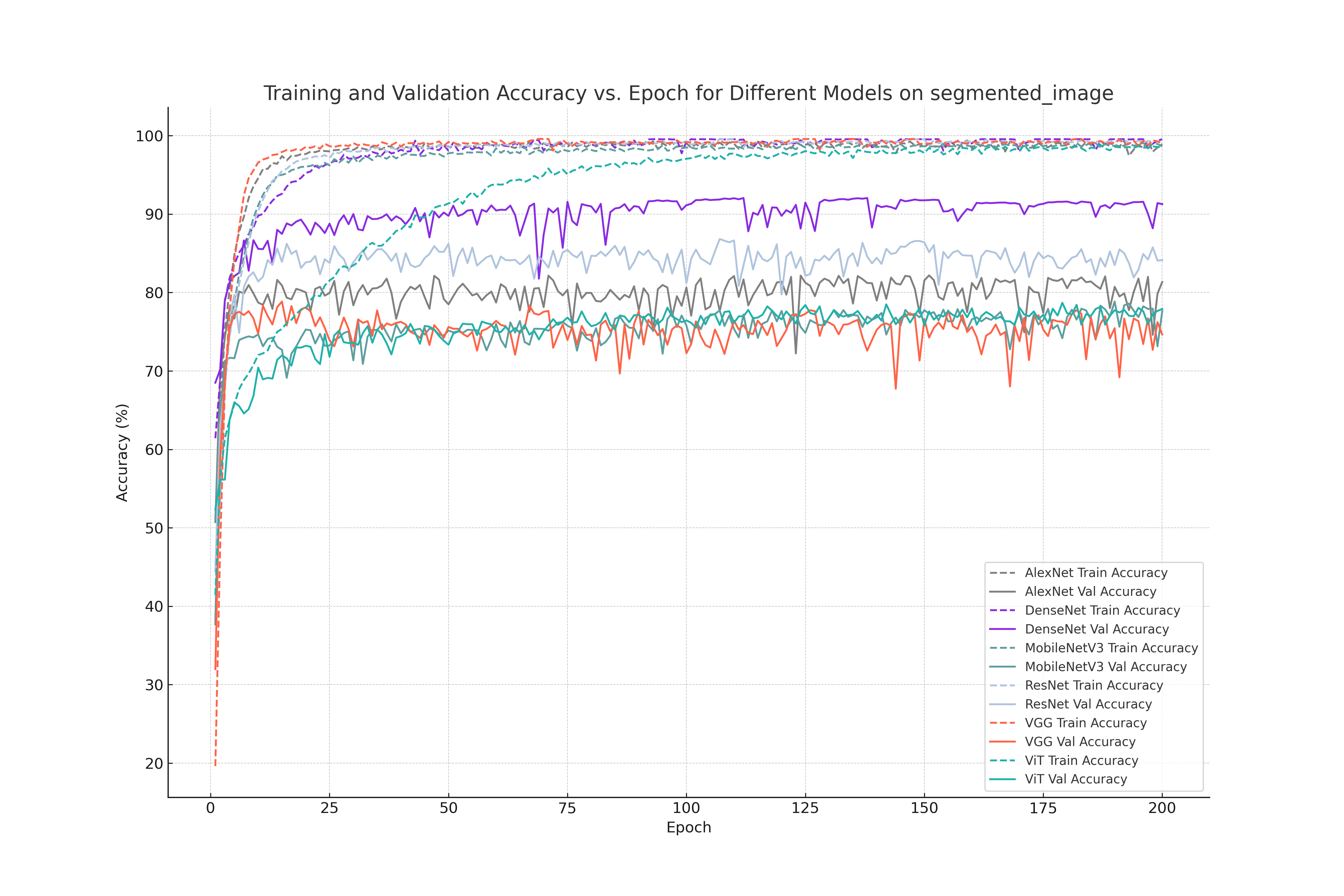
Top-1 training and validation accuracy on the segmented scenario

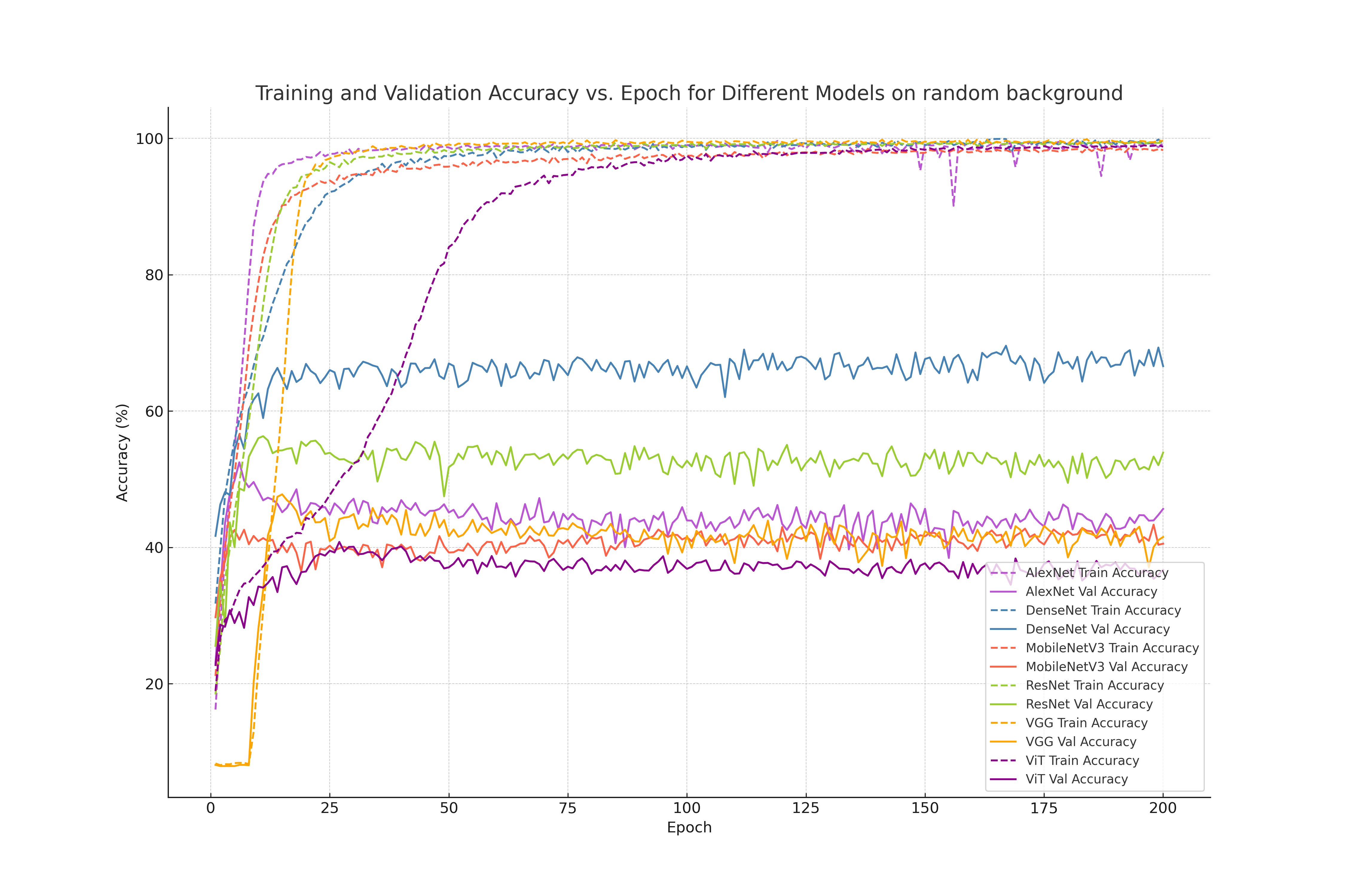
Top-1 training and validation accuracy on random background-generated scenario

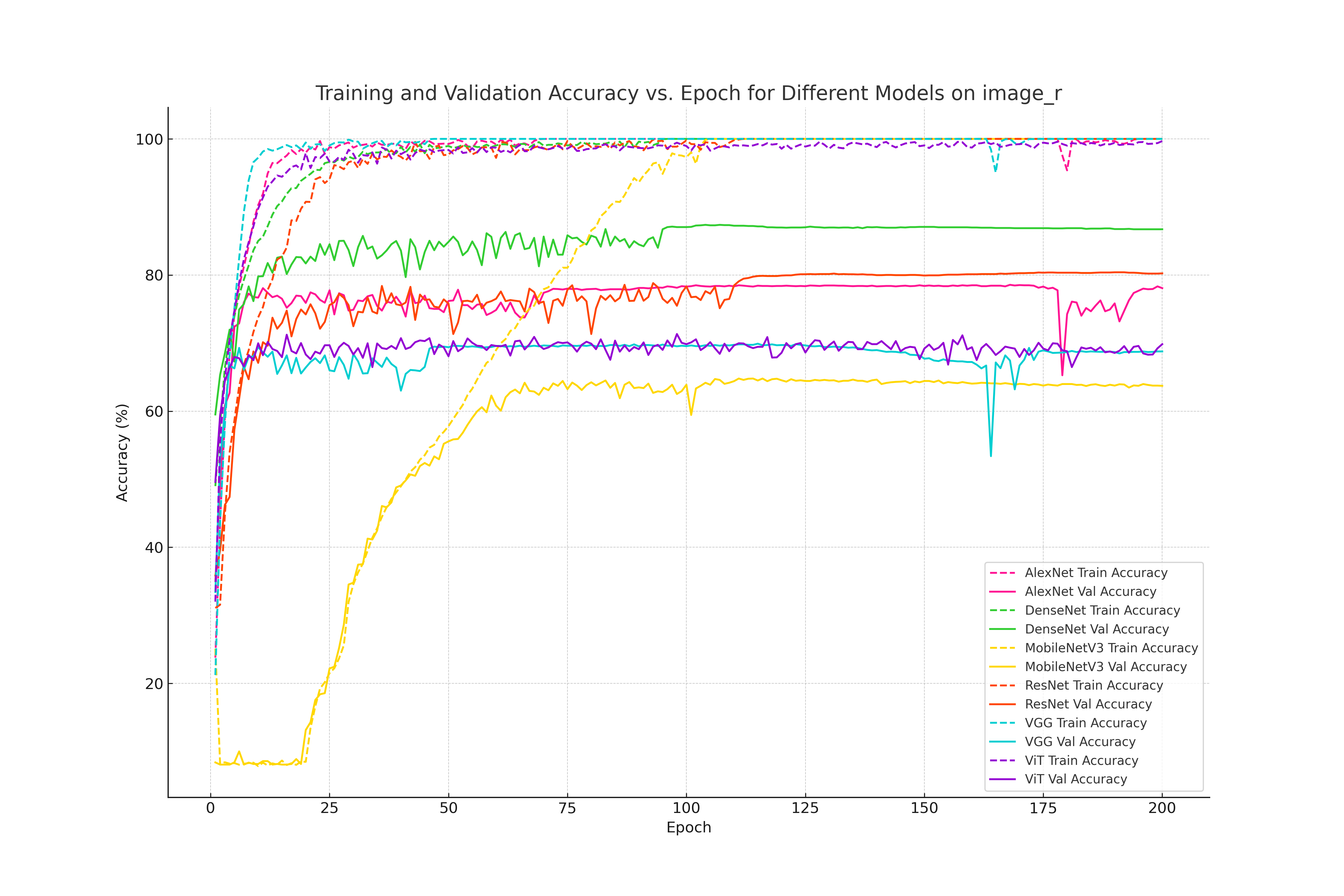
Top-1 training and validation accuracy on only one red channel generated scenario

Figure 8: Top-1 training and validation accuracy for SOTA models on Experiment 2.

However, it’s important to note that Transformer-based models, including ViT [29], have limitations in terms of speed and resource requirements. When processing images of the same resolution and batch size see Fig. 3 and Fig. 8, these models demand nearly twice the training time and GPU resources compared to other architectures. Consequently, there is a pressing need to develop Vision Transformers that are optimized for high-resolution images and industrial scenarios, striking a balance between accuracy and latency.

3.3 Results And Finding: EX2

We used mainstream classification models ResNet [25], VGG [37], AlexNet [38], MobileNet [26], and Vit [29] to train and test the within our scenarios. As shown in Fig.2, we can notice that after learning scenarios through fine-tuning, we observed a significant improvement in classification accuracy. Different models exhibit varying degrees of responsiveness to image transformations, with ViT [29] and DenseNet121 [28] demonstrating better robustness. An intriguing observation is that employing reasonable image segmentation masks does not significantly hinder image classification results; in fact, it might even enhance classification accuracy. This finding aligns with some prior research, such as [40], which noted that models trained and tested with well-segmented foregrounds tend to exhibit improved performance. Therefore, we propose that the assertion in the work of [11], regarding a decrease in classification accuracy due to segmentation may be contingent on the quality of the segmentation rather than an inherent negative impact of segmentation on classification performance, see Fig.6.

3.4 Results And Finding: EX3

Here, we conducted a regression analysis to assess segmentation accuracy. Our reference model was Deeplabv3plus [36] R50-D8, and the fundamental images served as the baseline. We ran seven segmentation experiments, including state-of-the-art models like Deeplabv3plus [36] R50-D8 and Upernet [32] models with ViT-B16 [29] and LN-MLN [30] transformers. For detailed segmentation accuracy data, refer to the Tab.6. Our regression analysis demonstrated a significant relationship between variables and segmentation accuracy, with highly significant F-statistics $P<0.0001$. Introducing a generated background scenario led to a 14.08% accuracy decrease compared to the original scenario. Specifically, the DPT ViT [29] B16 model had a 19.99% accuracy decrease, the Upernet Swin [32] model showed a 22.11% decrease, the Upernet ViT B16 LN MLN [32] model had a 16.95% decrease, the FPN [35] R50 model exhibited a 20.81% decrease compared to the reference model.

4 Our robustness Scores framework

In general, we face the challenge of lacking a standard reference for evaluating the robustness scores of visual models. Currently, most methods rely on testing these models on well-known benchmarks, often leading researchers to test on more and more datasets [18, 19]. However, testing on additional datasets doesn’t necessarily make a model more robust. Importantly, these methods can assess a model’s generalization performance but cannot verify its performance in different scenarios, such as changes in lighting, blurring, or background noise. Moreover, while precision and recall have clear mathematical formalizations, robustness lacks a similar formalization. Therefore, inspired by the mathematical definitions of variance and covariance, we have developed robustness scores based on our explainable benchmarks, as follows:

$$(\sigma_{e})^{2}=\frac{\sum_{i=1}^{n}(C(i)-\mu)^{2}}{n}$$

, where $\mu$ is Expect Best Weight Acc. namely, best test Accuracy on the original image with pre-trained under original scenarios, with respect to $n$ ( scenarios number, such as blur, color…).

$$(\sigma_{i})^{2}=\frac{\sum_{k=1}^{n}(C^{\prime}(k)-\mu)^{2}}{n}$$

where $\{0,1,\dots,n\}$ represents the set of all target object subclasses between $0$ and $n$, and $\mu$ denotes the Expected Best Weight Accuracy, i.e., the best test accuracy on the original image under original scenarios. In the end, Robustness can be categorized into two key aspects: Internal scenario object class robustness, which pertains to sensitivity to different classes of objects, such as animals and humans, etc. External scenario robustness signifies the ability to maintain stability amidst changing background conditions for the same objects:

$$S_{\text{robust}}=1-(\sigma_{i}+\sigma_{e})$$

In addition to its statistical usage, ”variance” is a term employed in the realm of for example finance. In finance, stock analysts and financial advisors employ variance to gauge a stock’s volatility or level of uncertainty. We also made significant comparisons for three types of classification models using our robustness score in Tab.3.

5 Ablation study: comparing on existing benchmark

There has been prior work on mitigating contextual bias in image classification [41], the influence of background signals on various datasets, and techniques like foreground segmentation that we leverage. In the realm of image backgrounds, prior studies have uncovered the predictive nature of background correlations [42]. These investigations have also shed light on the varying degrees to which backgrounds can impact model decisions [43, 44].

Our research shares commonalities with the work of Zhu, Xie, and Yuille [43], and Xiao Kai [11] who delved into ImageNet classification and segmentation, and background exploration. However, we’ve taken several significant steps forward: (a) we provide a comprehensive toolkit for measuring model robustness across six scenarios, (b) we’ve enhanced semantic labeling quality and introduced cross-validation to eliminate noise and inaccuracies, (c) we investigate model robustness against adversarial backgrounds, and (d) we consider a wider array of contemporary image classifiers. In essence, our study contributes to a deeper comprehension of content understanding by incorporating modern models and examining diverse factors influencing their predictions.

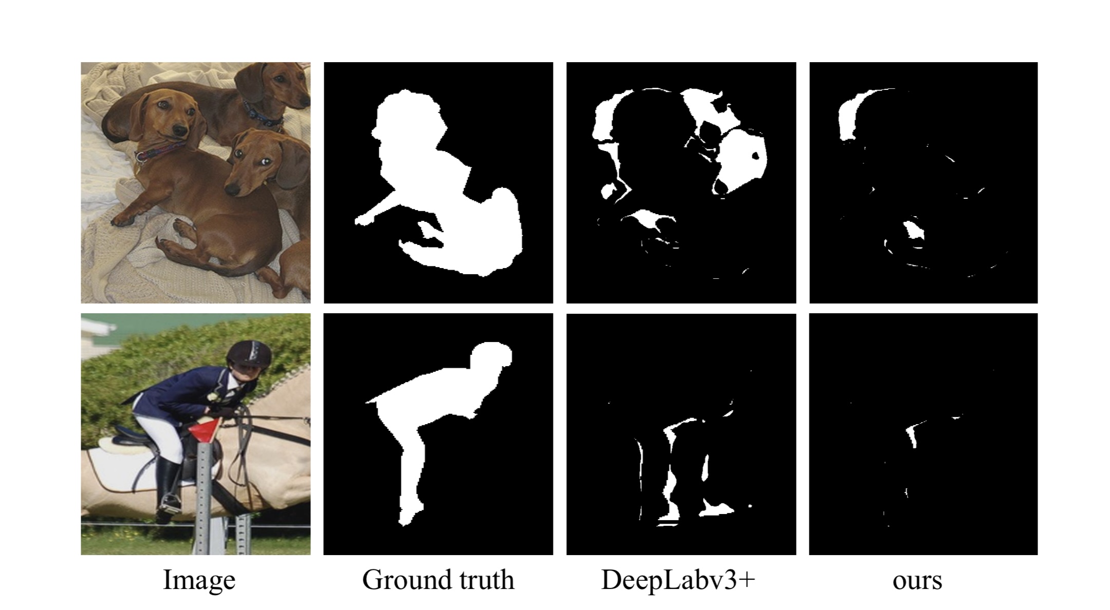
(a) IoG Benchmark Dataset

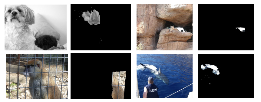
(b) ImageNet-9 Dataset

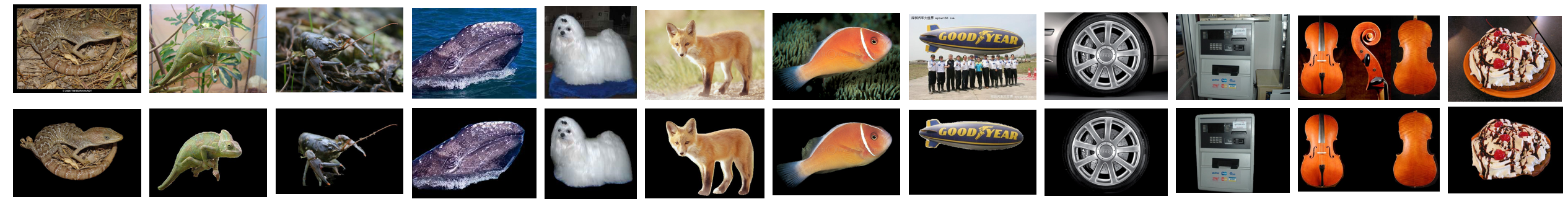
(c) Our XIMAGENET-12 mask samples

Figure 6: Additional Related Works and Explicit Comparisons.

6 DISCUSSION AND CONCLUSION

In conclusion, the motivation behind the creation of this dataset stems from our experiences with anomaly detection models deployed in industry projects. Through these deployments, we have encountered various unexpected scenarios where model performance was challenged. Our primary objective in developing this dataset was to bridge the gap between academia and industry. By offering an explainable AI dataset XIMAGENET-12 where the target object remains consistent while the background introduces noise or undergoes alterations, and an easily comprehensible robustness scoring mechanism, we enable researchers and practitioners to evaluate and enhance the true robustness of their models in context. In essence, this dataset serves as a critical tool to help the industry and academia collaborate effectively, ensuring that computer vision models are not only accurate in controlled settings but also capable of withstanding the complexities and uncertainties.

7 Appendix

Table 3: Variance of Model Accuracy Performance and Robustness Scores.

Model Acc. Drop Volatility	Scenarios								Variance	Robustness Score (Our* 0 - 1)	Offical Top-1 Acc. (On ImageNet)
	Blur_background	Blur_object	Image_g	Image_b	Image_grey	Image_r	Random_background	Segmented_image
ResNet50 [25]: external	0,18%	0,50%	1,17%	0,68%	0,10%	0,38%	53,04%	7,12%	0,0902	0,8985	74,90%
ResNet50 [25]: internal	0,10%	0,00%	0,11%	0,17%	0,20%	0,00%	6,96%	0,30%	0,0112
DenseNet121 [28]:external	0,13%	0,72%	1,00%	1,01%	0,17%	0,84%	50,39%	7,69%	0,0885	0,9062	75,00%
DenseNet121 [28]:internal	0,21%	0,00%	0,07%	0,14%	0,18%	0,01%	2,77%	0,29%	0,0052
VGG-16 [37]:external	0,15%	0,15%	2,30%	5,45%	1,52%	1,72%	47,93%	19,53%	0,1125	0,8845	71,30%
VGG-16 [37]:internal	0,33%	0,06%	0,26%	0,51%	0,72%	0,01%	0,01%	0,17%	0,0029
ViT [29]:external	0,25%	0,07%	7,60%	9,38%	5,18%	7,24%	58,11%	19,74%	0,1536	0,8196	81,07%
ViT [29]:internal	0,51%	0,72%	0,15%	0,07%	0,08%	0,57%	16,54%	0,00%	0,0266

Table 4: Analysis of Variance and Parameter Estimates.

Analysis of Variance	EX1				EX3
	SS	DF	MS	F (DFn, DFd) / P value	SS	DF	MS	F (DFn, DFd) / P value
Regression	25.76	23	1.12	F (23, 516) = 99.40 / $<0.0001$	17.47	25	0.6989	F (25, 730) = 41.95 / $<0.0001$
Model Name	0.2761	4	0.06903	F (4, 516) = 6.125 / $<0.0001$	5.418	6	0.9029	F (6, 730) = 54.20 / $<0.0001$
Image Scenario	23.19	8	2.899	F (8, 516) = 257.2 / $<0.0001$	2.4	8	0.3	F (8, 730) = 18.01 / $<0.0001$
Image Class	2.298	11	0.2089	F (11, 516) = 18.54 / $<0.0001$	9.655	11	0.8777	F (11, 730) = 52.68 / $<0.0001$
Residual	5.815	516	0.01127		12.16	730	0.01666
Total	31.58	539			29.63	755

Table 5: Classification Accuracy Density Map of DenseNet121 [28], pretrained on ImageNet, Test on XImageNet12. This table contains the content for the DenseNet121 [28] model results with the density map-like color scale for accuracy.

Model Name	Background Scenarios	Class Name
		0	1	2	3	4	5	6	7	8	9	10	11
DenseNet121 [28]	blur_background	0.95	0.97	0.89	0.93	0.93	0.96	0.89	0.91	0.98	0.93	0.99	0.92
	blur_object	0.74	0.91	0.72	0.91	0.93	0.94	0.73	0.95	0.94	0.96	0.98	0.97
	image_g	0.81	0.93	0.75	0.68	0.89	0.94	0.9	0.92	0.9	0.98	0.98	0.8
	image_b	0.71	0.77	0.75	0.82	0.96	0.97	0.93	0.89	0.96	0.89	0.96	0.87
	image_grey	0.94	0.93	0.83	0.81	0.98	0.97	0.95	0.98	0.9	0.98	0.97	0.95
	image_r	0.87	0.87	0.82	0.92	0.97	0.96	0.94	0.85	0.92	0.89	0.97	0.57
	Random Background with Real Environment	0.3	0.32	0.2	0.39	0.16	0.32	0.09	0.07	0.14	0.46	0.63	0.07
	Segmented_image	0.63	0.85	0.67	0.51	0.91	0.83	0.73	0.62	0.75	0.69	0.95	0.16
	Original	0.96	0.97	0.93	0.97	0.98	0.98	0.97	0.99	0.99	0.98	0.98	0.99

(a) ResNet50 74.9%

(b) DenseNet 78.8%

(c) MobileNet 70.9%

Figure 9: Model accuracy for classifying normal/AI-generated/random-generated images.

Table 6: Multiple linear regression performance of Experiment 3 on Model about Segmentation Tasks.

Variable	Estimate	Standard error	95% CI (asymptotic)	P value	P value summary
Intercept	0.6672	0.02394	0.6202 to 0.7142	$<0.0001$	****
Model Name[dpt_vit-b16 [29]]	-0.1999	0.01756	-0.2344 to -0.1654	$<0.0001$	****
Model Name[upernet_swin [32]]	-0.2211	0.01756	-0.2556 to -0.1866	$<0.0001$	****
Model Name[upernet_vit-b16 _ln_mln[32]]	-0.1695	0.01756	-0.2040 to -0.1351	$<0.0001$	****
Model Name[pspnet_r50-d8 [34]]	-0.045	0.01756	-0.07948 to -0.01052	0.0106	*
Model Name[fpn_r50 [35]]	-0.2081	0.01756	-0.2426 to -0.1737	$<0.0001$	****
Model Name[upernet_r50 [32]]	-0.05796	0.01756	-0.09245 to -0.02348	0.001	**
Image Scenario[blur_background]	0.01833	0.01992	-0.02077 to 0.05743	0.3576	ns
Image Scenario[blur_object]	-0.1571	0.01992	-0.1962 to -0.1180	$<0.0001$	****
Image Scenario[image_g]	-0.07131	0.01992	-0.1104 to -0.03221	0.0004	***
Image Scenario[image_b]	-0.03952	0.01992	-0.07862 to -0.0004243	0.0476	*
Image Scenario[image_grey]	-0.01929	0.01992	-0.05839 to 0.01981	0.3332	ns
Image Scenario[image_r]	-0.07702	0.01992	-0.1161 to -0.03792	$0.0001$	***
Image Scenario[segmented_image]	-0.08143	0.01992	-0.1205 to -0.04233	$<0.0001$	****
Image Scenario[generated_background]	-0.1408	0.01992	-0.1799 to -0.1017	$<0.0001$	****
Image Class[1]	0.07619	0.023	0.03104 to 0.1213	0.001	***
Image Class[2]	-0.06508	0.023	-0.1102 to -0.01993	0.0048	**
Image Class[3]	0.05222	0.023	0.007074 to 0.09737	0.0234	*
Image Class[4]	0.08127	0.023	0.03612 to 0.1264	0.0004	***
Image Class[5]	0.2713	0.023	0.2261 to 0.3164	$<0.0001$	****
Image Class[6]	0.3021	0.023	0.2569 to 0.3472	$<0.0001$	****
Image Class[7]	0.1641	0.023	0.1190 to 0.2093	$7.137$	****
Image Class[8]	0.1548	0.023	0.1096 to 0.1999	$6.73$	****
Image Class[9]	0.2216	0.023	0.1764 to 0.2667	$9.635$	****
Image Class[10]	0.2689	0.023	0.2237 to 0.3140	$11.69$	****
Image Class[11]	0.04079	0.023	-0.004355 to 0.08594	$1.774$	ns

References

- [1] Haonan Han, Rui Yang, Shuyan Li, Runze Hu, and Xiu Li. Ssgd: A smartphone screen glass dataset for defect detection. In ICASSP 2023 - 2023 IEEE International Conference on Acoustics, Speech and Signal Processing (ICASSP), pages 1–5, 2023.
- [2] Fangfang Zhou, Zhengming Fu, and Dan Zhang. High dynamic range imaging with context-aware transformer. In 2023 International Joint Conference on Neural Networks (IJCNN), pages 1–8. IEEE, 2023.
- [3] Evrim Ozmermer and Qiang Li. Self-supervised learning with temporary exact solutions: Linear projection. In 2023 IEEE 21st International Conference on Industrial Informatics (INDIN), pages 1–7. IEEE, 2023.
- [4] Qiang Li and Chongyu Zhang. Continual learning on deployment pipelines for machine learning systems. In In 36th Conference on Neural Information Processing Systems (NeurIPS 2022). DMML Workshop, 2022.
- [5] Jie Zhang, Masanori Suganuma, and Takayuki Okatani. Network pruning and fine-tuning for few-shot industrial image anomaly detection. In 2023 IEEE 21st International Conference on Industrial Informatics (INDIN), pages 1–6, 2023.
- [6] Ziyu Jia, Youfang Lin, Yuhan Zhou, Xiyang Cai, Peng Zheng, Qiang Li, and Jing Wang. Exploiting interactivity and heterogeneity for sleep stage classification via heterogeneous graph neural network. In IEEE International Conference on Acoustics, Speech and Signal Processing (ICASSP), 2023.
- [7] Dan Zhang, Fangfang Zhou, Yuwen Jiang, and Zhengming Fu. Mm-bsn: Self-supervised image denoising for real-world with multi-mask based on blind-spot network. In Proceedings of the IEEE/CVF Conference on Computer Vision and Pattern Recognition, pages 4188–4197, 2023.
- [8] Jia Deng, Wei Dong, Richard Socher, Li-Jia Li, Kai Li, and Li Fei-Fei. Imagenet: A large-scale hierarchical image database. In 2009 IEEE conference on computer vision and pattern recognition, pages 248–255. Ieee, 2009.
- [9] Andrew D Selbst and Solon Barocas. The intuitive appeal of explainable machines. Fordham L. Rev., 87:1085, 2018.
- [10] Shiyin Zhang, Jun Hao Liew, Yunchao Wei, Shikui Wei, and Yao Zhao. Interactive object segmentation with inside-outside guidance. In Proceedings of the IEEE/CVF conference on computer vision and pattern recognition, pages 12234–12244, 2020.
- [11] Kai Xiao, Logan Engstrom, Andrew Ilyas, and Aleksander Madry. Noise or signal: The role of image backgrounds in object recognition. arXiv preprint arXiv:2006.09994, 2020.
- [12] Ziniu Hu, Yuxiao Dong, Kuansan Wang, Kai-Wei Chang, and Yizhou Sun. Gpt-gnn: Generative pre-training of graph neural networks. In Proceedings of the 26th ACM SIGKDD International Conference on Knowledge Discovery & Data Mining, pages 1857–1867, 2020.
- [13] Dong-Hyun Lee et al. Pseudo-label: The simple and efficient semi-supervised learning method for deep neural networks. In Workshop on challenges in representation learning, ICML, volume 3, page 896. Atlanta, 2013.
- [14] Qizhe Xie, Minh-Thang Luong, Eduard Hovy, and Quoc V Le. Self-training with noisy student improves imagenet classification. In Proceedings of the IEEE/CVF conference on computer vision and pattern recognition, pages 10687–10698, 2020.
- [15] Xieyuanli Chen, Benedikt Mersch, Lucas Nunes, Rodrigo Marcuzzi, Ignacio Vizzo, Jens Behley, and Cyrill Stachniss. Automatic labeling to generate training data for online lidar-based moving object segmentation. IEEE Robotics and Automation Letters, 7(3):6107–6114, 2022.
- [16] Ziyang Wang and Irina Voiculescu. Weakly supervised medical image segmentation through dense combinations of dense pseudo-labels. In MICCAI Workshop on Data Engineering in Medical Imaging, pages 1–10. Springer, 2023.
- [17] Robin Rombach, Andreas Blattmann, Dominik Lorenz, Patrick Esser, and Björn Ommer. High-resolution image synthesis with latent diffusion models. In Proceedings of the IEEE/CVF conference on computer vision and pattern recognition, pages 10684–10695, 2022.
- [18] Norman Mu and Justin Gilmer. Mnist-c: A robustness benchmark for computer vision. arXiv preprint arXiv:1906.02337, 2019.
- [19] Oliver Zendel, Wolfgang Herzner, and Markus Murschitz. Vitro-model based vision testing for robustness. In IEEE ISR 2013. IEEE, 2013.
- [20] Antonio Torralba and Alexei A Efros. Unbiased look at dataset bias. In CVPR 2011, pages 1521–1528. IEEE, 2011.
- [21] Samuel Dodge and Lina Karam. Understanding how image quality affects deep neural networks. In 2016 eighth international conference on quality of multimedia experience (QoMEX), pages 1–6. IEEE, 2016.
- [22] Jifeng Dai, Yi Li, Kaiming He, and Jian Sun. R-fcn: Object detection via region-based fully convolutional networks. Advances in neural information processing systems, 29, 2016.
- [23] Dustin Podell, Zion English, Kyle Lacey, Andreas Blattmann, Tim Dockhorn, Jonas Müller, Joe Penna, and Robin Rombach. Sdxl: improving latent diffusion models for high-resolution image synthesis. arXiv preprint arXiv:2307.01952, 2023.
- [24] PlaygroundAI. playgroundai, 2023.
- [25] Kaiming He, Xiangyu Zhang, Shaoqing Ren, and Jian Sun. Deep residual learning for image recognition. In Proceedings of the IEEE conference on computer vision and pattern recognition, pages 770–778, 2016.
- [26] Mark Sandler, Andrew Howard, Menglong Zhu, Andrey Zhmoginov, and Liang-Chieh Chen. Mobilenetv2: Inverted residuals and linear bottlenecks. In Proceedings of the IEEE conference on computer vision and pattern recognition, pages 4510–4520, 2018.
- [27] Mingxing Tan and Quoc Le. Efficientnet: Rethinking model scaling for convolutional neural networks. In International conference on machine learning, pages 6105–6114. PMLR, 2019.
- [28] Gao Huang, Zhuang Liu, Laurens Van Der Maaten, and Kilian Q Weinberger. Densely connected convolutional networks. In Proceedings of the IEEE conference on computer vision and pattern recognition, pages 4700–4708, 2017.
- [29] Alexey Dosovitskiy, Lucas Beyer, Alexander Kolesnikov, Dirk Weissenborn, Xiaohua Zhai, Thomas Unterthiner, Mostafa Dehghani, Matthias Minderer, Georg Heigold, Sylvain Gelly, et al. An image is worth 16x16 words: Transformers for image recognition at scale. arXiv preprint arXiv:2010.11929, 2020.
- [30] Kai Chen, Jiaqi Wang, Jiangmiao Pang, Yuhang Cao, Yu Xiong, Xiaoxiao Li, Shuyang Sun, Wansen Feng, Ziwei Liu, Jiarui Xu, et al. Mmdetection: Open mmlab detection toolbox and benchmark. arXiv preprint arXiv:1906.07155, 2019.
- [31] Liang-Chieh Chen, Yukun Zhu, George Papandreou, Florian Schroff, and Hartwig Adam. Encoder-decoder with atrous separable convolution for semantic image segmentation. In Proceedings of the European conference on computer vision (ECCV), pages 801–818, 2018.
- [32] Tete Xiao, Yingcheng Liu, Bolei Zhou, Yuning Jiang, and Jian Sun. Unified perceptual parsing for scene understanding. In Proceedings of the European conference on computer vision (ECCV), pages 418–434, 2018.
- [33] Ze Liu, Yutong Lin, Yue Cao, Han Hu, Yixuan Wei, Zheng Zhang, Stephen Lin, and Baining Guo. Swin transformer: Hierarchical vision transformer using shifted windows. In Proceedings of the IEEE/CVF international conference on computer vision, pages 10012–10022, 2021.
- [34] Hengshuang Zhao, Jianping Shi, Xiaojuan Qi, Xiaogang Wang, and Jiaya Jia. Pyramid scene parsing network. In Proceedings of the IEEE conference on computer vision and pattern recognition, pages 2881–2890, 2017.
- [35] Tsung-Yi Lin, Piotr Dollár, Ross Girshick, Kaiming He, Bharath Hariharan, and Serge Belongie. Feature pyramid networks for object detection. In Proceedings of the IEEE conference on computer vision and pattern recognition, pages 2117–2125, 2017.
- [36] Liang-Chieh Chen, George Papandreou, Florian Schroff, and Hartwig Adam. Rethinking atrous convolution for semantic image segmentation. arXiv preprint arXiv:1706.05587, 2017.
- [37] Karen Simonyan and Andrew Zisserman. Very deep convolutional networks for large-scale image recognition. arXiv preprint arXiv:1409.1556, 2014.
- [38] Alex Krizhevsky, Ilya Sutskever, and Geoffrey E Hinton. Imagenet classification with deep convolutional neural networks. Advances in neural information processing systems, 25, 2012.
- [39] Andrew Howard, Mark Sandler, Grace Chu, Liang-Chieh Chen, Bo Chen, Mingxing Tan, Weijun Wang, Yukun Zhu, Ruoming Pang, Vijay Vasudevan, et al. Searching for mobilenetv3. In Proceedings of the IEEE/CVF international conference on computer vision, pages 1314–1324, 2019.
- [40] Otesteanu Corin and Qiang Li. All you need is cell attention: A cell annotation tool for single-cell morphology data. In The Ninth International Conference on Learning Representation (ICLR), AI for Public Health Workshop, 2021.
- [41] Ruohan Gao, Rogerio Feris, and Kristen Grauman. Learning to separate object sounds by watching unlabeled video. In Proceedings of the European Conference on Computer Vision (ECCV), pages 35–53, 2018.
- [42] Antonio Torralba. Contextual priming for object detection. International journal of computer vision, 53:169–191, 2003.
- [43] Zhuotun Zhu, Lingxi Xie, and Alan L Yuille. Object recognition with and without objects. arXiv preprint arXiv:1611.06596, 2016.
- [44] Marco Tulio Ribeiro, Sameer Singh, and Carlos Guestrin. ” why should i trust you?” explaining the predictions of any classifier. In Proceedings of the 22nd ACM SIGKDD international conference on knowledge discovery and data mining, pages 1135–1144, 2016.