Elimination of QCD Renormalization Scale and Scheme Ambiguities

Abstract

We present results for the thrust distribution in the electron positron annihilation to the three jet process at NNLO in the perturbative conformal window of QCD, as a function of the number of flavors $N_{f}$. Given the existence of an infrared interacting fixed point in this region, we can compare the Conventional Scale Setting (CSS) and the Principle of Maximum Conformality (PMC_∞) methods along the entire renormalization group flow from the highest energies to zero energy. We then consider also the QED thrust, obtained as the limit $N_{c}\rightarrow 0$ of the number of colors and we show analogous comparison. QED in the low energy regime develops an infrared non-interacting fixed point. Using these quantum field theory limits as theoretical laboratories, we arrive at interesting results showing new features of the PMC_∞.

1 Introduction

The renormalization scale and scheme ambiguities are important sources of errors, which greatly affect the results of the Conventional Scale Setting (CSS) in perturbative QCD calculations. Given the high precision reached by the experiments at LEP and SLAC [1, 2, 3, 4, 5] in the measurement of the event shape variables and accuracy achieved by higher order calculations from next-to-leading order (NLO) calculations [6, 7, 8, 9, 10, 11] to the next-to-next-to-leading order(NNLO) [12, 13, 14, 15, 16] and including resummation of the large logarithms [17, 18], the elimination of the uncertainties related to the scheme and scale ambiguities is crucial in order to improve the results and to test the Standard Model to the highest possible precision. In the particular case of the three-jet event-shape distributions the conventional practice of CSS leads to results which are in conflict with experimental data and the extracted values of $\alpha_{s}$ deviate from the world average [19]. A solution to the renormalization scale ambiguity problem is provided by the Principle of Maximum Conformality (PMC) [20, 21, 22, 23, 24, 25, 26, 27, 28]. This method provides a systematic way to eliminate renormalization scheme-and-scale ambiguities from first principles by absorbing the $\beta$ terms that govern the behavior of the running coupling via the renormalization group equation. This procedure is scheme-independent and leads to results free from divergent renormalon terms [29]. The PMC procedure is consistent with the standard Gell-Mann–Low method in the Abelian limit, $N_{c}\rightarrow 0$ [30] and can be considered the non-Abelian extension of the Serber–Uehling [31, 32] scale setting, which is essential for precision tests of QED and atomic physics. It should be emphasized that in a theory of unification of all forces, electromagnetic, weak and strong interactions, such as the Standard Model, or Grand Unification theories, one cannot simply apply a different scale-setting or analytic procedure to different sectors of the theory. The PMC offers the possibility to apply the same method in all sectors of a theory, starting from first principles, eliminating the renormalon growth, the scheme dependence, scale ambiguities while satisfying the QED Gell-Mann-Low scale-setting in the zero-color limit $N_{c}\to 0$. We remark that PMC leads to scheme invariant results. We refer to RS-scheme invariance as the invariance under the extended-renormalization group and its equations (xRGE). Any other relation among different quantities defined in different approximations or obtained using different approaches, that can have perturbative validity in QCD, can be improved using the PMC and the residual dependence on the particular definition of the "scheme" can be suppressed perturbatively by adding higher order calculations. It can be shown that also in this case the results obtained are scheme-independent (see Ref. [37]). We remark that in order to apply the PMC correctly, one should be able to distinguish among the nature of the different $n_{f}$-terms, whether they are related to the running of the coupling, to the running of masses or to UV-finite diagrams and in a deeper analysis also to the particular UV-divergent diagram (as discussed in Refs. [39, 40]). Once all $n_{f}$-terms have been associated with the correct diagram or parameter, conformal coefficients are RG invariant and match the coefficients of a conformal theory. Moreover, given that the PMC preserves the RG invariance, it is possible to define CSR - Commensurate Scale Relations[25] among the effective charges relating observables in different "schemes" preserving all the group properties. Applying the PMC and the CSRs, one can relate effective couplings, as also conformal coefficients, leading to scheme independent results for the observables. Applications of the PMC to different quantities (see Ref. [41, 42]) have recently shown a direct improvement of theoretical predictions. The recently developed Infinite-Order Scale-Setting using the Principle of Maximum Conformality (PMC_∞) has been shown to significantly reduce the theoretical errors in Event Shape Variable distributions, highly improving also the fit with the experimental data[39, 43, 44, 45]. An improved theoretical prediction on $\alpha_{s}$ with respect to the world average has also been shown in Refs.[46, 47]. In this article we consider the thrust distribution in the region of flavors and colors near the upper bound of the conformal window, i.e. $N_{f}\sim 11/2N_{c}$ , where the IR fixed point can be reliably accessed in perturbation theory and we compare the two renormalization scale setting methods, the CSS and the PMC_∞. In this region we are able to deduce the full solution at NNLO in the strong coupling. We also compare the two methods in the QED, $N_{c}\rightarrow 0$, limit of thrust.

2 Two-loop solution and the perturbative conformal window

The strong coupling dependence on the scale can be described introducing the $\beta$-function given by:

$$\frac{1}{4\pi}\frac{d\alpha_{s}(Q^{2})}{d\log Q^{2}}=\beta(\alpha_{s}),$$ (1)

and

$$\beta\left(\alpha_{s}\right)=-\left(\frac{\alpha_{s}}{4\pi}\right)^{2}\sum_{n=0}\left(\frac{\alpha_{s}}{4\pi}\right)^{n}\beta_{n}.$$ (2)

Neglecting quark masses, the first two $\beta$-terms are RS independent and they have been calculated in Refs. [48, 49, 50, 51, 52] for the $\overline{\rm MS}$ scheme:

$$\beta_{0} = \frac{11}{3}C_{A}-\frac{4}{3}T_{R}N_{f},$$ (3)

$$\beta_{1} = \frac{34}{3}C_{A}^{2}-4\left(\frac{5}{3}C_{A}+C_{F}\right)T_{R}N_{f},$$ (4)

where $C_{F}=\frac{\left(N_{c}^{2}-1\right)}{2N_{c}}$, $C_{A}=N_{c}$ and $T_{R}=1/2$ are the color factors for the ${\rm SU(3)}$ gauge group [53].
In order to determine the solution for the strong coupling $\alpha_{s}$ at NNLO, it is convenient to introduce the following notation: $x(\mu)\equiv\frac{\alpha_{s}(\mu)}{2\pi}$, $t=\log(\mu^{2}/\mu_{0}^{2})$, $B=\frac{1}{2}\beta_{0}$ and $C=\frac{1}{2}\frac{\beta_{1}}{\beta_{0}}$, $x^{*}\equiv-\frac{1}{C}$. The truncated NNLO approximation of the Eq. 1 leads to the differential equation:

$$\frac{dx}{dt}=-Bx^{2}(1+Cx).$$ (5)

An implicit solution of Eq. 5 is given by the Lambert $W(z)$ function:

$$We^{W}=z,$$ (6)

with: $W=\left(\frac{x^{*}}{x}-1\right)$. The general solution for the coupling is:

$$x = \frac{x^{*}}{1+W},$$ (7)

$$z = e^{\frac{x^{*}}{x_{0}}-1}\left(\frac{x^{*}}{x_{0}}-1\right)\left(\frac{\mu^{2}}{\mu_{0}^{2}}\right)^{x^{*}B}.$$ (8)

We shall discuss here the solutions to Eq. 5 with respect to the particular initial phenomenological value $x_{0}\equiv\alpha_{s}(M_{Z})/(2\pi)=0.01876\pm 0.00016$ given by the coupling determined at the $Z^{0}$ mass scale [19]. This value introduces an upper boundary on the number of flavors: $\bar{N}_{f}=x^{*-1}(x_{0})=15.222\pm 0.009$, which narrows the range for the IR fixed point discussed by Banks and Zaks [54]. The only physically accessible range is $N_{f}<\bar{N}_{f}$, since for $N_{f}>\bar{N}_{f}$ we no longer have the asymptotically free UV behavior. In the range $N_{f}<\bar{N_{f}^{1}}$ we have $B>0$, $C>0$ and the physical solution is given by the $W_{-1}$ branch, while for $\bar{N_{f}^{1}}<N_{f}<\bar{N_{f}}$ the solution for the strong coupling is given by the $W_{0}$ branch. Where the values $\bar{N_{f}^{0}}=\frac{11}{2}N_{c}$, $\bar{N_{f}^{1}}=\frac{34N_{c}^{3}}{13N_{c}^{2}-3}$, with $\bar{N_{f}^{0}}>\bar{N_{f}^{1}}$, are the zeros of $\beta_{0},\beta_{1}$ respectively. The two-dimensional region in the number of flavors and colors where asymptotically free QCD develops an IR interacting fixed point is colloquially known as the conformal window of pQCD. Different solutions for the NNLO equation can be achieved using different schemes, i.e. different definitions of the $\Lambda$ scale parameter, as shown in Ref. [55]. In general, IR and UV fixed points of the $\beta$-function can also be determined at different values of the number of colors $N_{c}$ (different gauge group $SU(N)$) and $N_{f}$ extending this analysis also to other gauge theories [56]. An extension of the perturbative QCD coupling and its $\beta$-function in the IR region can be found in Ref. [57].

3 The thrust distribution according to $N_{f}$

The thrust distribution and the event shape variables are a fundamental tool in order to probe the geometrical structure of a given process at colliders and for the measurement of the strong coupling $\alpha_{s}$ [58]. Thrust ($T$) is defined as

$$T=\max\limits_{\vec{n}}\left(\frac{\sum_{i}|\vec{p}_{i}\cdot\vec{n}|}{\sum_{i}|\vec{p}_{i}|}\right),$$ (9)

where the sum runs over all particles in the hadronic final state, and $\vec{p}_{i}$ denotes the three-momentum of particle $i$. The unit vector $\vec{n}$ is varied to maximize thrust $T$, and the corresponding $\vec{n}$ is called the thrust axis and denoted by $\vec{n}_{T}$. The variable $(1-T)$ is often used, which for the LO of 3-jet production is restricted to the range $(0<1-T<1/3)$. We have a back-to-back or a spherically symmetric event respectively at $T=1$ and at $T=2/3$ respectively.

In general, a normalized IR-safe single-variable observable, such as the thrust distribution for the $e^{+}e^{-}\rightarrow 3jets$ [59, 60], is the sum of pQCD contributions calculated up to NNLO at the initial renormalization scale $\mu_{0}=\sqrt{s}=M_{Z}$:

$$\frac{1}{\sigma_{tot}}\!\frac{Od\sigma(\mu_{0})}{dO}\! = \left\{x_{0}\cdot\frac{Od\overline{A}_{\mathit{O}}(\mu_{0})}{dO}+x_{0}^{2}\cdot\frac{Od\overline{B}_{\mathit{O}}(\mu_{0})}{dO}\right.$$ (10)

$$+\left.x_{0}^{3}\cdot\frac{Od\overline{C}_{\mathit{O}}(\mu_{0})}{dO}+{\cal O}(\alpha_{s}^{4})\right\}$$

where $x(\mu)\equiv\alpha_{s}(\mu)/(2\pi)$, $O$ is the selected event shape variable, $\sigma$ the cross section of the process,

$$\sigma_{tot}=\sigma_{0}\left(1+x_{0}A_{tot}+x_{0}^{2}B_{tot}+{\cal O}\left(\alpha_{s}^{3}\right)\right),$$ (11)

is the total hadronic cross section and $\overline{A}_{O},\overline{B}_{O},\overline{C}_{O}$ are respectively the normalized LO, NLO and NNLO coefficients:

$$\overline{A}_{O} = A_{O},$$

$$\overline{B}_{O} = B_{O}-A_{tot}A_{O},$$ (12)

$$\overline{C}_{O} = C_{O}-A_{tot}B_{O}-\left(B_{tot}-A_{tot}^{2}\right)A_{O},$$

where $A_{O},B_{O},C_{O}$ are the coefficients normalized to the tree-level cross section $\sigma_{0}$ calculated by MonteCarlo (see e.g. the EERAD and Event2 codes [12, 13, 14, 15, 16]) and $A_{\mathit{tot}},B_{\mathit{tot}}$ are:

$$A_{\mathit{tot}} = \frac{3}{2}C_{F},$$

$$B_{\mathit{tot}} = \frac{C_{F}}{4}N_{c}+\frac{3}{4}C_{F}\frac{\beta_{0}}{2}(11-8\zeta(3))-\frac{3}{8}C_{F}^{2},$$ (13)

where $\zeta$ is the Riemann zeta function. In the case of conventional scale setting, the renormalization scale is set to $\mu_{0}=\sqrt{s}=M_{Z}$ and theoretical uncertainties are evaluated using standard criteria. In this case, we have used the definition given in Ref. [13] of the parameter $\delta$; we define the average error for the event shape variable distributions as:

$$\bar{\delta}=\frac{1}{N}\sum_{i}^{N}\frac{{\rm max}_{\mu}(\sigma_{i}(\mu))-{\rm min}_{\mu}(\sigma_{i}(\mu))}{2\sigma_{i}(\mu=M_{Z})},$$ (14)

where $i$ is the index of the bin and $N$ is the total number of bins, the renormalization scale is varied in the range: $\mu\in[M_{Z}/2;2M_{Z}]$. We use here the two-loop solution for the running coupling $\alpha_{s}(Q)$. According to the PMC_∞ (for a detailed analysis see Ref. [39, 44, 45]), Eq. 10 becomes:

$$\frac{1}{\sigma_{tot}}\!\frac{Od\sigma(\mu_{\rm I},\tilde{\mu}_{\rm II},\mu_{0})}{dO}=\left\{\overline{\sigma}_{\rm I}+\overline{\sigma}_{\rm II}+\overline{\sigma}_{\rm III}+{\cal O}(\alpha_{s}^{4})\right\},$$ (15)

where the $\overline{\sigma}_{N}$ are normalized subsets given by:

$$\overline{\sigma}_{\rm I} = A_{\mathit{Conf}}\cdot x_{\rm I},$$

$$\overline{\sigma}_{\rm II} = \left(B_{\mathit{Conf}}+\eta A_{\mathit{tot}}A_{\mathit{Conf}}\right)\cdot x_{\rm II}^{2}-\eta A_{\textrm{tot}}A_{\mathit{Conf}}\cdot x_{0}^{2}$$

$$\hskip 65.44142pt-A_{\textrm{tot}}A_{\mathit{Conf}}\cdot x_{0}x_{\rm I},$$

$$\overline{\sigma}_{\rm III} = \!\!\left(C_{\mathit{Conf}}\!-\!A_{\textrm{tot}}\!B_{\mathit{Conf}}\!-\!(B_{\textrm{tot}}-A_{\textrm{tot}}^{2})A_{\mathit{Conf}}\right)\cdot x_{0}^{3},$$ (16)

where $A_{\mathit{Conf}},B_{\mathit{Conf}},C_{\mathit{Conf}}$ are the scale-invariant conformal coefficients (i.e. the coefficients of each perturbative order not depending on the scale $\mu_{R}$) while $x_{\rm I},x_{\rm II},x_{0}$ are the couplings determined at the PMC_∞ scales: $\mu_{\rm I},\tilde{\mu}_{\rm II},M_{Z}$ respectively. The PMC_∞ scales are given by:

$$\large{\mu}_{\rm I} = \sqrt{s}\cdot e^{f_{sc}-\frac{1}{2}B_{\beta_{0}}}\hskip 99.58464pt{\scriptstyle(1-T)<0.33},$$ (17)

$$\large{\tilde{\mu}}_{\rm II} = \left\{\begin{array}[]{lr}\sqrt{s}\cdot e^{f_{sc}-\frac{1}{2}C_{\beta_{0}}\cdot\frac{B_{\mathit{Conf}}}{B_{\mathit{Conf}}+\eta\cdot A_{\mathit{tot}}A_{\mathit{Conf}}}}&{\scriptstyle(1-T)<0.33},\\ \sqrt{s}\cdot e^{f_{sc}-\frac{1}{2}C_{\beta_{0}}},&{\scriptstyle(1-T)>0.33},\\ \end{array}\right.$$ (20)

where the $f_{sc}$ is a general scheme factor which is $f_{sc}\equiv 0$ for the QCD case in $\overline{\rm MS}$-scheme. Normalized subsets for the region $(1-T)>0.33$ can be simply achieved by setting $A_{\mathit{Conf}}\equiv 0$ in the Eq. 16. Results for the thrust distribution calculated using the NNLO solution for the coupling $\alpha_{s}(\mu)$, at different values of the number of flavors, $N_{f}$, is shown in Fig. 1.

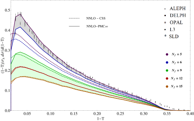
Figure 1: Thrust distributions for different values of $N_{f}$, using the PMC_∞ (solid line) and the CSS (dashed line) [45]. The Green shaded area is the results for the values of $N_{f}$ taken in the conformal window. The experimental data points are taken from the ALEPH, DELPHI,OPAL, L3, SLD experiments [1, 2, 3, 4, 5].

A direct comparison between PMC_∞ (solid line) and CSS (dashed line) is shown at different values of the number of flavors. We notice that, despite the phase transition (i.e. the transition from an infrared finite coupling to an infrared divergent coupling), the curves given by the PMC_∞ at different $N_{f}$, preserve with continuity the same characteristics of the conformal distribution setting $N_{f}$ out of the conformal window of pQCD. We notice that by decreasing $N_{f}$, the peak increases and this is mainly due to larger values of the $\beta_{0},\beta_{1}$ coefficients, obtaining a better match with the data for values in the range $5\leq N_{f}\leq 6$. The position of the peak of the thrust distribution is well preserved varying $N_{f}$ in and out of the conformal window using the PMC_∞, while there is constant shift towards lower values using the CSS. These trends are shown in Fig. 2. We notice that in the central range, $2<N_{f}<15$, the position of the peak is exactly preserved using the PMC_∞ and overlaps with the position of the peak shown by the experimental data. Theoretical uncertainties on the position of the peak have been calculated using standard criteria, i.e. varying the remaining initial scale value in the range $M_{Z}/2\leq\mu_{0}\leq 2M_{Z}$, and considering the lowest uncertainty given by the half of the spacing between two adjacent bins.

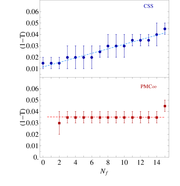
Figure 2: Comparison of the position of the peak for the thrust distribution using the CSS and the PMC_∞ vs the number of flavors, $N_{f}$. Dashed lines indicate the particular trend in each graph [45].

Using the definition given in Eq. 14, we have determined the average error, $\bar{\delta}$, calculated in the interval $0.005<(1-T)<0.4$ of thrust and results for CSS and PMC_∞ are shown in Fig. 3. We notice that the PMC_∞ in the perturbative and IR conformal window, i.e. $12<N_{f}<\bar{N}_{f}$, which is the region where $\alpha_{s}(\mu)<1$ in the whole range of the renormalization scale values, from $0$ up to $\infty$, the average error given by PMC_∞ tends to zero ($\sim 0.23-0.26\%$) while the error given by the CSS tends to remain constant ($0.85-0.89\%$). The comparison of the two methods shows that, out of the conformal window, $N_{f}<\frac{34N_{c}^{3}}{13N_{c}^{2}-3}$, the PMC_∞ leads to a higher precision.

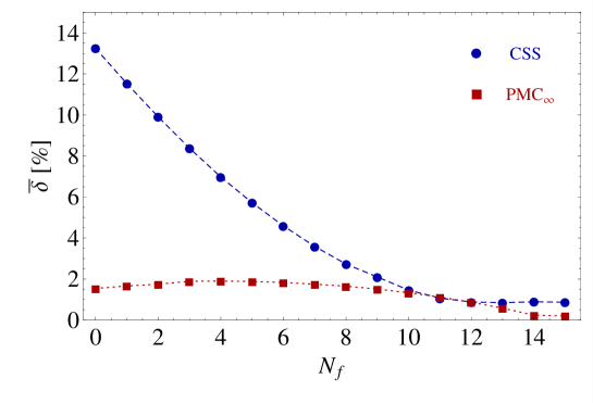
Figure 3: Comparison of the average theoretical error, $\bar{\delta}$, calculated using standard criteria in the range: $0.005<(1-T)<0.4$, using the CSS and the PMC_∞ for the thrust distribution vs the number of flavors, $N_{f}$ [45].

4 The thrust distribution in the Abelian limit $N_{c}\rightarrow 0$

We consider now the thrust distribution in U(1) Abelian QED, which rather than being infrared interacting is infrared free. We obtain the QED thrust distribution performing the $N_{c}\rightarrow 0$ limit of the QCD thrust at NNLO according to [30, 61]. In the zero number of colors limit the gauge group color factors are fixed by $N_{A}=1,$ $C_{F}=1,$ $T_{R}=1,$ $C_{A}=0,$ $N_{c}=0,$ $N_{f}=N_{l}$, where $N_{l}$ is the number of active leptons, while the $\beta$-terms and the coupling rescale as $\beta_{n}/C_{F}^{n+1}$ and $\alpha_{s}\cdot C_{F}$ respectively. In particular $\beta_{0}=-\frac{4}{3}N_{l}$ and $\beta_{1}=-4N_{l}$ using the normalization of Eq. 1. According to this rescaling of the color factors we have determined the QED thrust and the QED PMC_∞ scales. For the QED coupling, we have used the analytic formula for the effective fine structure constant in the $\overline{\textrm{MS}}$-scheme:

$${\alpha(Q^{2})}={\alpha\over{\left(1-\Re e\Pi^{\overline{\textrm{MS}}}(Q^{2})\right)}},$$ (21)

with $\alpha^{-1}\equiv\alpha(0)^{-1}=137.036$ and the vacuum polarization function ($\Pi$) calculated perturbatively at two loops including contributions from leptons, quarks and $W$ boson. The QED PMC_∞ scales have the same form of Eqs. 17 and LABEL:icfscale2 with the factor for the $\overline{\textrm{MS}}$-scheme set to $f_{sc}\equiv 5/6$ and the $\eta$ regularization parameter introduced to cancel singularities in the NLO PMC_∞ scale $\mu_{\rm II}$ in the $N_{c}\rightarrow 0$ limit tends to the same QCD value, $\eta=3.51$. A direct comparison between QED and QCD PMC_∞ scales is shown in Fig. 4.

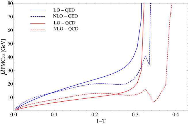
Figure 4: PMC_∞ scales for the thrust distribution: LO-QCD scale (solid red); LO-QED scale (solid blue);NLO-QCD scale (dashed red); NLO-QED scale (dashed blue) [45].

We note that in the QED limit the PMC_∞ scales have analogous dynamical behavior as those calculated in QCD, differences arise mainly owing to the $\overline{\textrm{MS}}$ scheme factor reabsorption, the effects of the $N_{c}$ number of colors at NLO are also negligible. Thus we notice that perfect consistency is shown from QCD to QED using the PMC_∞ method. The normalized QED thrust distribution is shown in Fig. 5. We note that the curve is peaked at the origin, $T=1$, which suggests that the three-jet event in QED occurs with a rather back-to-back symmetry. Results for the CSS and the PMC_∞ methods in QED are of the order of $O(\alpha)$ and show very small differences, given the good convergence of the theory.

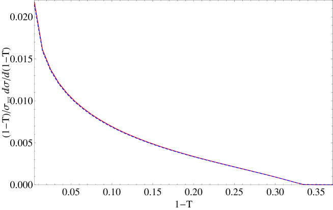
Figure 5: Thrust distributions in the QED limit at NNLO using the PMC_∞ (solid red) and the CSS (dashed blue) [45].

5 Conclusion

We have investigated for the first time the thrust distribution within the perturbative conformal window of QCD and in QED and we have compared results obtained using both the CSS and the PMC_∞ scale setting. In the latter case the results are in perfect agreement with the Gell-Man–Low scheme. Results for different values of the $N_{f}$ factor show that the PMC_∞ scale setting leads to higher precision and are in agreement with the data in a wide range of the selected event shape variable. Moreover the thrust distributions in the conformal window have similar shapes to those of the physical values of $N_{f}$ and the position of the peak is preserved when one applies the PMC_∞ method. Thus, even though the peak is a property directly related to the resummation of the large-logarithms in the low-energy region [62, 63, 64, 65, 66, 17], the correct position of the peak can be considered in fact a conformal property and it can be related to the use of the PMC_∞ scales.

References

- [1] A. Heister et al. [ALEPH], Eur. Phys. J. C 35, 457-486 (2004) doi:10.1140/epjc/s2004-01891-4
- [2] J. Abdallah et al. [DELPHI], Eur. Phys. J. C 29, 285-312 (2003) doi:10.1140/epjc/s2003-01198-0 [arXiv:hep-ex/0307048 [hep-ex]].
- [3] G. Abbiendi et al. [OPAL], Eur. Phys. J. C 40, 287-316 (2005) doi:10.1140/epjc/s2005-02120-6 [arXiv:hep-ex/0503051 [hep-ex]].
- [4] P. Achard et al. [L3], Phys. Rept. 399, 71-174 (2004) doi:10.1016/j.physrep.2004.07.002 [arXiv:hep-ex/0406049 [hep-ex]].
- [5] K. Abe et al. [SLD], Phys. Rev. D 51, 962-984 (1995) doi:10.1103/PhysRevD.51.962 [arXiv:hep-ex/9501003 [hep-ex]].
- [6] R. K. Ellis, D. A. Ross and A. E. Terrano, Nucl. Phys. B 178, 421-456 (1981) doi:10.1016/0550-3213(81)90165-6
- [7] Z. Kunszt, Phys. Lett. B 99, 429-432 (1981) doi:10.1016/0370-2693(81)90563-3
- [8] J. A. M. Vermaseren, K. J. F. Gaemers and S. J. Oldham, Nucl. Phys. B 187, 301-320 (1981) doi:10.1016/0550-3213(81)90276-5
- [9] K. Fabricius, I. Schmitt, G. Kramer and G. Schierholz, Z. Phys. C 11, 315 (1981) doi:10.1007/BF01578281
- [10] W. T. Giele and E. W. N. Glover, Phys. Rev. D 46, 1980-2010 (1992) doi:10.1103/PhysRevD.46.1980
- [11] S. Catani and M. H. Seymour, Phys. Lett. B 378, 287-301 (1996) doi:10.1016/0370-2693(96)00425-X [arXiv:hep-ph/9602277 [hep-ph]].
- [12] A. Gehrmann-De Ridder, T. Gehrmann, E. W. N. Glover and G. Heinrich, Comput. Phys. Commun. 185, 3331 (2014) doi:10.1016/j.cpc.2014.07.024 [arXiv:1402.4140 [hep-ph]].
- [13] A. Gehrmann-De Ridder, T. Gehrmann, E. W. N. Glover and G. Heinrich, Phys. Rev. Lett. 99, 132002 (2007) doi:10.1103/PhysRevLett.99.132002 [arXiv:0707.1285 [hep-ph]].
- [14] A. Gehrmann-De Ridder, T. Gehrmann, E. W. N. Glover and G. Heinrich, JHEP 12, 094 (2007) doi:10.1088/1126-6708/2007/12/094 [arXiv:0711.4711 [hep-ph]].
- [15] S. Weinzierl, Phys. Rev. Lett. 101, 162001 (2008) doi:10.1103/PhysRevLett.101.162001 [arXiv:0807.3241 [hep-ph]].
- [16] S. Weinzierl, JHEP 06, 041 (2009) doi:10.1088/1126-6708/2009/06/041 [arXiv:0904.1077 [hep-ph]].
- [17] R. Abbate, M. Fickinger, A. H. Hoang, V. Mateu and I. W. Stewart, Phys. Rev. D 83, 074021 (2011) doi:10.1103/PhysRevD.83.074021 [arXiv:1006.3080 [hep-ph]].
- [18] A. Banfi, H. McAslan, P. F. Monni and G. Zanderighi, JHEP 05, 102 (2015) doi:10.1007/JHEP05(2015)102 [arXiv:1412.2126 [hep-ph]].
- [19] R. L. Workman et al. [Particle Data Group], PTEP 2022, 083C01 (2022) doi:10.1093/ptep/ptac097
- [20] S. J. Brodsky, G. P. Lepage and P. B. Mackenzie, Phys. Rev. D 28, 228 (1983) doi:10.1103/PhysRevD.28.228
- [21] S. J. Brodsky and L. Di Giustino, Phys. Rev. D 86, 085026 (2012) doi:10.1103/PhysRevD.86.085026 [arXiv:1107.0338 [hep-ph]].
- [22] S. J. Brodsky and X. G. Wu, Phys. Rev. D 85, 034038 (2012) [erratum: Phys. Rev. D 86, 079903 (2012)] doi:10.1103/PhysRevD.85.034038 [arXiv:1111.6175 [hep-ph]].
- [23] S. J. Brodsky and X. G. Wu, Phys. Rev. Lett. 109, 042002 (2012) doi:10.1103/PhysRevLett.109.042002 [arXiv:1203.5312 [hep-ph]].
- [24] M. Mojaza, S. J. Brodsky and X. G. Wu, Phys. Rev. Lett. 110, 192001 (2013) doi:10.1103/PhysRevLett.110.192001 [arXiv:1212.0049 [hep-ph]].
- [25] S. J. Brodsky, M. Mojaza and X. G. Wu, Phys. Rev. D 89, 014027 (2014) doi:10.1103/PhysRevD.89.014027 [arXiv:1304.4631 [hep-ph]].
- [26] S. J. Brodsky and X. G. Wu, Phys. Rev. D 86, 054018 (2012) doi:10.1103/PhysRevD.86.054018 [arXiv:1208.0700 [hep-ph]].
- [27] X. G. Wu, Y. Ma, S. Q. Wang, H. B. Fu, H. H. Ma, S. J. Brodsky and M. Mojaza, Rept. Prog. Phys. 78, 126201 (2015) doi:10.1088/0034-4885/78/12/126201 [arXiv:1405.3196 [hep-ph]].
- [28] S. Q. Wang, S. J. Brodsky, X. G. Wu, J. M. Shen and L. Di Giustino, Universe 9, no.4, 193 (2023) doi:10.3390/universe9040193 [arXiv:2302.08153 [hep-ph]].
- [29] M. Beneke, Phys. Rept. 317, 1-142 (1999) doi:10.1016/S0370-1573(98)00130-6 [arXiv:hep-ph/9807443 [hep-ph]].
- [30] S. J. Brodsky and P. Huet, Phys. Lett. B 417, 145-153 (1998) doi:10.1016/S0370-2693(97)01209-4 [arXiv:hep-ph/9707543 [hep-ph]].
- [31] R. Serber, Phys. Rev. 48, 49 (1935) doi:10.1103/PhysRev.48.49
- [32] E. A. Uehling, Phys. Rev. 48, 55-63 (1935) doi:10.1103/PhysRev.48.55
- [33] P. M. Stevenson, [arXiv:2308.05072 [hep-ph]].
- [34] P. M. Stevenson, Phys. Rev. D 23, 2916 (1981) doi:10.1103/PhysRevD.23.2916
- [35] Y. Ma, X. G. Wu, H. H. Ma and H. Y. Han, Phys. Rev. D 91, no.3, 034006 (2015) doi:10.1103/PhysRevD.91.034006 [arXiv:1412.8514 [hep-ph]].
- [36] Y. Ma and X. G. Wu, Phys. Rev. D 97, no.3, 036024 (2018) doi:10.1103/PhysRevD.97.036024 [arXiv:1707.09886 [hep-ph]].
- [37] X. G. Wu, J. M. Shen, B. L. Du and S. J. Brodsky, Phys. Rev. D 97, no.9, 094030 (2018) doi:10.1103/PhysRevD.97.094030 [arXiv:1802.09154 [hep-ph]].
- [38] X. G. Wu, J. M. Shen, B. L. Du, X. D. Huang, S. Q. Wang and S. J. Brodsky, Prog. Part. Nucl. Phys. 108, 103706 (2019) doi:10.1016/j.ppnp.2019.05.003 [arXiv:1903.12177 [hep-ph]].
- [39] L. Di Giustino, S. J. Brodsky, P. G. Ratcliffe, X. G. Wu and S. Q. Wang, [arXiv:2307.03951 [hep-ph]].
- [40] L. Di Giustino, [arXiv:2205.03689 [hep-ph]].
- [41] X. D. Huang, J. Yan, H. H. Ma, L. Di Giustino, J. M. Shen, X. G. Wu and S. J. Brodsky, Nucl. Phys. B 989, 116150 (2023) doi:10.1016/j.nuclphysb.2023.116150 [arXiv:2109.12356 [hep-ph]].
- [42] S. Q. Wang, S. J. Brodsky, X. G. Wu, L. Di Giustino and J. M. Shen, Phys. Rev. D 102, no.1, 014005 (2020) doi:10.1103/PhysRevD.102.014005 [arXiv:2002.10993 [hep-ph]].
- [43] S. Q. Wang, C. Q. Luo, X. G. Wu, J. M. Shen and L. Di Giustino, JHEP 09, 137 (2022) doi:10.1007/JHEP09(2022)137 [arXiv:2112.06212 [hep-ph]].
- [44] L. Di Giustino, S. J. Brodsky, S. Q. Wang and X. G. Wu, Phys. Rev. D 102, no.1, 014015 (2020) doi:10.1103/PhysRevD.102.014015 [arXiv:2002.01789 [hep-ph]].
- [45] L. Di Giustino, F. Sannino, S. Q. Wang and X. G. Wu, Phys. Lett. B 823, 136728 (2021) doi:10.1016/j.physletb.2021.136728 [arXiv:2104.12132 [hep-ph]].
- [46] S. Q. Wang, S. J. Brodsky, X. G. Wu and L. Di Giustino, Phys. Rev. D 99, no.11, 114020 (2019) doi:10.1103/PhysRevD.99.114020 [arXiv:1902.01984 [hep-ph]].
- [47] S. Q. Wang, S. J. Brodsky, X. G. Wu, J. M. Shen and L. Di Giustino, Phys. Rev. D 100, no.9, 094010 (2019) doi:10.1103/PhysRevD.100.094010 [arXiv:1908.00060 [hep-ph]].
- [48] D. J. Gross and F. Wilczek, Phys. Rev. Lett. 30, 1343-1346 (1973) doi:10.1103/PhysRevLett.30.1343
- [49] H. D. Politzer, Phys. Rev. Lett. 30, 1346-1349 (1973) doi:10.1103/PhysRevLett.30.1346
- [50] W. E. Caswell, Phys. Rev. Lett. 33, 244 (1974) doi:10.1103/PhysRevLett.33.244
- [51] D. R. T. Jones, Nucl. Phys. B 75, 531 (1974) doi:10.1016/0550-3213(74)90093-5
- [52] E. Egorian and O. V. Tarasov, Teor. Mat. Fiz. 41, 26-32 (1979) JINR-E2-11757.
- [53] M. Mojaza, C. Pica and F. Sannino, Phys. Rev. D 82, 116009 (2010) doi:10.1103/PhysRevD.82.116009 [arXiv:1010.4798 [hep-ph]].
- [54] T. Banks and A. Zaks, Nucl. Phys. B 196, 189-204 (1982) doi:10.1016/0550-3213(82)90035-9
- [55] E. Gardi, G. Grunberg and M. Karliner, JHEP 07, 007 (1998) doi:10.1088/1126-6708/1998/07/007 [arXiv:hep-ph/9806462 [hep-ph]].
- [56] T. A. Ryttov and R. Shrock, Phys. Rev. D 96, no.10, 105018 (2017) doi:10.1103/PhysRevD.96.105018 [arXiv:1706.06422 [hep-th]].
- [57] S. J. Brodsky, G. F. de Teramond and A. Deur, Phys. Rev. D 81, 096010 (2010) doi:10.1103/PhysRevD.81.096010 [arXiv:1002.3948 [hep-ph]].
- [58] S. Kluth, Rept. Prog. Phys. 69, 1771-1846 (2006) doi:10.1088/0034-4885/69/6/R04 [arXiv:hep-ex/0603011 [hep-ex]].
- [59] V. Del Duca, C. Duhr, A. Kardos, G. Somogyi, Z. Szőr, Z. Trócsányi and Z. Tulipánt, Phys. Rev. D 94, no.7, 074019 (2016) doi:10.1103/PhysRevD.94.074019 [arXiv:1606.03453 [hep-ph]].
- [60] V. Del Duca, C. Duhr, A. Kardos, G. Somogyi and Z. Trócsányi, Phys. Rev. Lett. 117, no.15, 152004 (2016) doi:10.1103/PhysRevLett.117.152004 [arXiv:1603.08927 [hep-ph]].
- [61] A. L. Kataev and V. S. Molokoedov, Phys. Rev. D 92, no.5, 054008 (2015) doi:10.1103/PhysRevD.92.054008 [arXiv:1507.03547 [hep-ph]].
- [62] S. Catani, G. Turnock, B. R. Webber and L. Trentadue, Phys. Lett. B 263, 491-497 (1991) doi:10.1016/0370-2693(91)90494-B
- [63] S. Catani, L. Trentadue, G. Turnock and B. R. Webber, Nucl. Phys. B 407, 3-42 (1993) doi:10.1016/0550-3213(93)90271-P
- [64] S. Catani, M. L. Mangano, P. Nason and L. Trentadue, Nucl. Phys. B 478, 273-310 (1996) doi:10.1016/0550-3213(96)00399-9 [arXiv:hep-ph/9604351 [hep-ph]].
- [65] U. Aglietti, L. Di Giustino, G. Ferrera and L. Trentadue, Phys. Lett. B 651, 275-292 (2007) doi:10.1016/j.physletb.2007.06.034 [arXiv:hep-ph/0612073 [hep-ph]].
- [66] U. Aglietti, L. Di Giustino, G. Ferrera, A. Renzaglia, G. Ricciardi and L. Trentadue, Phys. Lett. B 653, 38-52 (2007) doi:10.1016/j.physletb.2007.07.041 [arXiv:0707.2010 [hep-ph]].