Structural Vector Autoregressions and Higher Moments: Challenges and Solutions in Small Samples.

Abstract

Generalized method of moments estimators based on higher-order moment conditions derived from independent shocks can be used to identify and estimate the simultaneous interaction in structural vector autoregressions. This study highlights two problems that arise when using these estimators in small samples. First, imprecise estimates of the asymptotically efficient weighting matrix and the asymptotic variance lead to volatile estimates and inaccurate inference. Second, many moment conditions lead to a small sample scaling bias towards innovations with a variance smaller than the normalizing unit variance assumption. To address the first problem, I propose utilizing the assumption of independent structural shocks to estimate the efficient weighting matrix and the variance of the estimator. For the second issue, I propose incorporating a continuously updated scaling term into the weighting matrix, eliminating the scaling bias. To demonstrate the effectiveness of these measures, I conducted a Monte Carlo simulation which shows a significant improvement in the performance of the estimator.

JEL Codes: C12, C32, C51
Keywords: structural vector autoregression, non-Gaussian, independent, GMM

1 Introduction

In non-Gaussian structural vector autoregressions (SVAR), higher-order moment conditions derived from mutually independent structural shocks can be used to identify the simultaneous relationship. These higher-order moment conditions can be used to estimate the SVAR with a generalized method of moments (GMM) estimator or similar moment-based estimators, see, e.g., Lanne and Luoto, (2021), Keweloh, (2021), Guay, (2021), Mesters and Zwiernik, (2022), Amengual et al., (2022), Karamysheva and Skrobotov, (2022), Lanne and Luoto, (2022), Lanne et al., (2022), Keweloh et al., (2023), or Drautzburg and Wright, (2023).

This study focuses on the small sample behavior of asymptotically efficient SVAR-GMM estimators based on higher-order moment conditions derived from mutually independent structural shocks. The results show that in small samples, standard implementations of GMM estimators lead to volatile and biased estimates with distorted coverage and Wald test statistics. To improve the small sample performance of the estimators, two extensions are proposed. First, the assumption of mutually independent structural shocks is used not only to derive moment conditions but also to estimate the asymptotically efficient weighting matrix and the asymptotic variance of the estimator. Second, a continuously updated scaling term is added to the weighting matrix to prevent the small sample scaling bias.

The small sample behavior of GMM estimators in general has been studied extensively and GMM estimators are known to exhibit a small sample bias, see, e.g., Han and Phillips, (2006) and Newey and Windmeijer, (2009). I prove that in the SVAR, the asymptotically efficient GMM estimator using higher-order moment conditions is biased towards solutions corresponding to innovations with a variance smaller than the normalizing unit variance assumption. This means that the normalizing unit variance moment conditions are systematically violated towards innovations with smaller variances. To address this scaling bias, I propose the continuous scale updating estimator (SVAR-CSUE), which eliminates the scaling bias by continuously updating the weighting matrix with a scaling term.

The estimation of the asymptotically efficient weighting matrix and the asymptotic variance of SVAR GMM estimators using higher-order moment conditions relies on estimates of the long-run covariance matrix of the sample average of the moment conditions, which is challenging to estimate due to the large number of higher-order moment conditions involved. For example, in an SVAR with two variables, independent shocks with unit variance imply eight moment conditions of order two to four and therefore, the covariance matrix of the moment conditions contains $35$ co-moments of order four to eight. However, in an SVAR with six variables, the number of moment conditions grows to $185$ and the covariance matrix explodes to $2919$ co-moments of order four to eight.

To solve the issue of the rapidly growing number of higher-order co-moments in the long-run covariance matrix, I propose leveraging the assumption of serially and mutually independent structural shocks, which is already used to derive the identifying moment conditions. This assumption enables the decomposition of higher-order co-moments of the covariance matrix into products of lower-order moments. For instance, in the SVAR with six variables and $185$ moment conditions of order two to four, the covariance matrix leveraging the assumption of serially and mutually independent shocks contains only $39$ moments of order one to six. Therefore, by leveraging this assumption to estimate the covariance matrix of the moment conditions, the researcher only needs to estimate moments up to order six instead of order eight, and the number of these moments increases linearly in the dimension of the SVAR, avoiding an explosion in the number of co-moments.

The study provides Monte Carlo simulations to demonstrate the effectiveness of the proposed measures. The simulations show that the proposed estimator of the efficient weighting matrix, leveraging the assumption of serially and mutually independent shocks, provides a substantially better approximation to the true asymptotically efficient weighting scheme than traditional approaches based on serially uncorrelated moment conditions. Moreover, the simulations show that the asymptotically efficient SVAR-GMM estimator exhibits a small sample scaling bias towards innovations with variances smaller than the normalizing unit variance assumption, which the proposed SVAR-CSUE, including a scale updating term, is shown to be effective in preventing. Additionally, the proposed SVAR-CSUE outperforms standard GMM implementations in terms of bias and volatility by correcting the scaling bias and additionally leveraging the assumption of serially and mutually independent shocks to estimate the efficient weighting matrix. Finally, leveraging the assumption of serially and mutually independent shocks to estimate the asymptotic variance of the estimator leads to substantially better coverage and rejection rates of Wald tests.

Hoesch et al., (2022) show that GMM-based Wald tests utilizing higher-order moment conditions tend to perform poorly and over-reject, particularly when dealing with weakly non-Gaussian shocks. To address this issue, Hoesch et al., (2022) and Drautzburg and Wright, (2023) propose Bonferroni-based approaches for hypothesis testing and constructing confidence sets, ensuring correct asymptotic coverage regardless of the level of non-Gaussianity. The simulations in this study show that GMM-based Wald tests relying on traditional approaches to estimate the asymptotic variance, i.e. based on serially uncorrelated moment conditions, may even severely over-reject in a setup with strongly non-Gaussian shocks featuring non-zero skewness and excess kurtosis. I demonstrate that a significant portion of the over-rejection issue stems from challenges in accurately estimating the asymptotic variance of the GMM estimator when employing higher-order moment conditions. Furthermore, the simulations reveal that by leveraging the assumption of serially and mutually independent shocks to estimate the asymptotic variance of the estimator, the issue can be alleviated, leading to considerably improved coverage and rejection rates for Wald tests. A notable advantage of the approach proposed in this study, compared to Bonferroni-based methods, is its computational efficiency, as it does not require inverting a test statistic. However, it is important to acknowledge that the proposed method may introduce potential distortions in setups with weak non-Gaussianity.

The remainder of this article is organized as follows. Section 2 contains an overview of SVAR identification and estimation using higher-order moment conditions implied by the assumption of independent structural shocks. Section 3 shows how the independence assumption can be leveraged to estimate the long-run covariance matrix of the moment conditions required for the asymptotically efficient weighting matrix and asymptotic variance of the SVAR-GMM estimator. Section 4 shows that the asymptotically efficient SVAR-GMM estimator using higher-order moment conditions exhibits a small sample scaling bias and proposes the SVAR-CSUE which prevents the scaling bias. Section 5 demonstrates the advantages of the two proposed measures in a Monte Carlo simulation. Section 6 concludes.

2 SVAR estimation using higher-order moment conditions

This section briefly summarizes how higher-order moment conditions derived from mutually independent structural shocks can be used to identify and estimate the SVAR. A detailed description can be found in Lanne and Luoto, (2021), Keweloh, (2021), Guay, (2021), or Lanne et al., (2022).

Consider the SVAR $y_{t}=\sum_{p=1}^{P}A_{p}y_{t-p}+u_{t}$ with an $n$-dimensional vector of observable variables $y_{t}=[y_{1,t},...,y_{n,t}]^{\prime}$, the reduced form shocks $u_{t}=[u_{1,t},...,u_{n,t}]^{\prime}$, and

$$u_{t} =B_{0}\varepsilon_{t}$$ (1)

describing the impact of an $n$-dimensional vector of unknown structural shocks $\varepsilon_{t}=[\varepsilon_{1,t},...,\varepsilon_{n,t}]^{\prime}$ with zero mean and unit variance. The matrix $B_{0}\in\mathbb{B}:=\{B\in\mathbb{R}^{n\times n}|det(B)\neq 0\}$ governs the simultaneous interaction and is assumed to be invertible. The reduced form shocks can be estimated consistently and this study focuses on the simultaneous interaction in Equation (1). The reduced form shocks are equal to an unknown mixture of the unknown structural shocks, $u_{t}=B_{0}\varepsilon_{t}$. Reversing this relationship yields the innovations $e(B)_{t}$, defined as the innovations obtained by unmixing the reduced form shocks with some invertible matrix $B$

$$e(B)_{t}:=B^{-1}u_{t}.$$ (2)

If $B$ is equal to the true mixing matrix $B_{0}$, the innovations are equal to the structural shocks.

Imposing structure on the (in-)dependencies of the structural form shocks allows deriving moment conditions. For example, if the structural shocks are mutually uncorrelated with unit variance, the unmixing matrix $B$ should yield uncorrelated innovations with unit variance and therefore, satisfy the second-order moment conditions in Table 1. However, there are not sufficiently many second-order moment conditions to identify the SVAR, which is the well-known identification problem. Imposing more structure on the (in-)dependencies of shocks allows for deriving additional higher-order moment conditions. In particular, if the structural form shocks are mutually independent, the innovations should additionally satisfy the third- and fourth-order moment conditions in Table 1.

Table 1: Illustration of moment conditions

covariance / second-order conditions	coskewness / third-order conditions
$\begin{matrix}E[\varepsilon_{1,t}^{2}]=1&\implies&E[e(B)_{1,t}^{2}]\overset{!}{=}1\\ &\vdots&\\ E[\varepsilon_{n,t}^{2}]=1&\implies&E[e(B)_{n,t}^{2}]\overset{!}{=}1\\ E[\varepsilon_{1,t}\varepsilon_{2,t}]=0&\implies&E[e(B)_{1,t}e(B)_{2,t}]\overset{!}{=}0\\ &\vdots&\end{matrix}$	$\begin{matrix}E[\varepsilon_{1,t}^{2}\varepsilon_{2,t}]=0&\implies&E[e(B)_{1,t}^{2}e(B)_{2,t}]\overset{!}{=}0\\ E[\varepsilon_{1,t}\varepsilon_{2,t}^{2}]=0&\implies&E[e(B)_{1,t}e(B)_{2,t}^{2}]\overset{!}{=}0\\ E[\varepsilon_{1,t}\varepsilon_{2,t}\varepsilon_{3,t}]=0&\implies&E[e(B)_{1,t}e(B)_{2,t}e(B)_{3,t}]\overset{!}{=}0\\ &\vdots&\end{matrix}$
cokurtosis / fourth-order conditions
$\begin{matrix}E[\varepsilon_{1,t}^{3}\varepsilon_{2,t}]=0&\implies&E[e(B)_{1,t}^{3}e(B)_{2,t}]\overset{!}{=}0\\ E[\varepsilon_{1,t}^{2}\varepsilon_{2,t}^{2}]=1&\implies&E[e(B)_{1,t}^{2}e(B)_{2,t}^{2}]\overset{!}{=}1\\ E[\varepsilon_{1,t}\varepsilon_{2,t}^{3}]=0&\implies&E[e(B)_{1,t}e(B)_{2,t}^{3}]\overset{!}{=}0\\ E[\varepsilon_{1,t}^{2}\varepsilon_{2,t}\varepsilon_{3,t}]=0&\implies&E[e(B)_{1,t}^{2}e(B)_{2,t}e(B)_{3,t}]\overset{!}{=}0\\ E[\varepsilon_{1,t}\varepsilon_{2,t}\varepsilon_{3,t}\varepsilon_{4,t}]=0&\implies&E[e(B)_{1,t}e(B)_{2,t}e(B)_{3,t}e(B)_{4,t}]\overset{!}{=}0\\ &\vdots&\end{matrix}$

In general, the moment conditions implied by mutually independent shocks with unit variance can be written as

$$E[f_{m}(B,u_{t})]=0\quad\text{with}\quad f_{m}(B,u_{t}):=\prod_{i=1}^{n}e(B)_{i,t}^{m_{i}}-c(m),$$ (3)

with variance and covariance conditions for $m\in\mathbf{2}$, coskewness conditions for $m\in\mathbf{3}$, and cokurtosis conditions for $m\in\mathbf{4}$ with

$$\mathbf{2}:=\{[ m_{1},....m_{n}]\in\{0,1,2\}^{n}|\sum_{i=1}^{n}m_{i}=2\},$$ (4)

$$\mathbf{3}:=\{[ m_{1},....m_{n}]\in\{0,1,2\}^{n}|\sum_{i=1}^{n}m_{i}=3\},$$ (5)

$$\mathbf{4}:=\{[ m_{1},....m_{n}]\in\{0,1,2,3\}^{n}|\sum_{i=1}^{n}m_{i}=4\},$$ (6)

and $c(m):=\begin{cases}0,&\text{if }1\in\{m_{1},....m_{n}\}\\ 1,&\text{else}\end{cases}$ .

In fact, all co-moment conditions except for the symmetric cokurtosis conditions $E[\varepsilon_{it}^{2}\varepsilon_{jt}^{2}]=1$ with $i\neq j$ can be derived under the weaker assumption of mutually mean independent shocks instead of the stronger assumption of mutually independent shocks. However, the weaker assumption may not be sufficient to ensure identification. For example, Lanne and Luoto, (2021), Keweloh, (2021), and Lanne and Luoto, (2022) propose different sets of identifying fourth-order moment conditions, nevertheless, all three identification results require the assumption that all cokurtosis conditions implied by independent shocks hold. Therefore, all three approaches are equally restrictive in terms of the structure imposed on the (in)dependencies of the shocks, and none of the proposed identification results using fourth-order moment conditions necessarily hold under the weaker assumption of mutually mean independent shocks.

Recently, several studies have made advancements in the identification of non-Gaussian SVAR models under the weaker assumption of mean independent shocks. Notably, Mesters and Zwiernik, (2022), Keweloh, (2023), and Anttonen et al., (2023) have provided identification results based on moment-based approaches. Keweloh, (2023) and Anttonen et al., (2023) employ third-order moment conditions, which enable the identification of SVAR models when the shocks exhibit sufficient skewness and zero co-skewness, a property derived from the assumption of mean independent shocks. On the other hand, Mesters and Zwiernik, (2022) present more general identification results that are not restricted to third-order moment conditions. However, despite these advancements, the simulations in Section 5 reveal that achieving efficient weighting of the higher-order moment conditions and accurate estimation of the asymptotic variances of the estimator can be challenging without relying on the assumption of independent structural shocks.

The remainder of the study uses the following assumptions:

Assumption 1.

1. The components of $\varepsilon_{t}$ are serially independent.

2. The components of $\varepsilon_{t}$ are mutually independent.

3. The components of $\varepsilon_{t}$ have zero mean, unit variance, and finite moments up to order eight.

The SVAR-GMM estimator is given by

$$\hat{B}_{T}:=\operatorname*{arg\,min}\limits_{B\in\mathbb{B}}g_{T}(B)^{\prime}Wg_{T}(B),$$ (7)

where $g_{T}(B)=\frac{1}{T}\sum_{t=1}^{T}f(B,u_{t})$, $W$ is a positive semi-definite weighting matrix, and $f(B,u_{t})$ contains all or a subset of the moment conditions $f_{m}(B,u_{t})$ implied by independence to ensure identification for sufficiently non-Gaussian shocks. Consistency and asymptotic normality of the estimator follow from standard assumptions, such that

$$\begin{matrix}\hat{\beta}_{T}\overset{p}{\rightarrow}\beta_{0}\\ \sqrt{T}(\hat{\beta}_{T}-\beta_{0})\overset{d}{\rightarrow}\mathcal{N}(0,MSM^{\prime})\end{matrix}\quad\text{with}\quad\begin{matrix}M:=\left(G^{\prime}S^{-1}G\right)^{-1}G^{\prime}W\\ G:=E\left[\frac{\partial f(B_{0},u_{t})}{\partial vec(B)^{\prime}}\right]\\ S:=\underset{T\rightarrow\infty}{lim}E\left[Tg_{T}(B_{0})g_{T}(B_{0})^{\prime}\right],\end{matrix}$$ (8)

with $\hat{\beta}_{T}=vec(\hat{B}_{T})$ and ${\beta}_{0}=vec({B}_{0})$, see Hall et al., (2005). In particular, asymptotic normality requires that the matrix $S$ exists and is finite. For the SVAR-GMM estimator based on second- to fourth-order moment conditions this requires that $\varepsilon_{t}$ has finite moments up to order eight. The weighting matrix $W^{*}:=S^{-1}$ leads to the estimator $\hat{B}_{T}^{*}$ with the asymptotic variance $\sqrt{T}(vec(\hat{B}_{T}^{*})-\beta_{0})\overset{d}{\rightarrow}\mathcal{N}(0,(G^{\prime}S^{-1}G)^{-1})$, which is the lowest possible asymptotic variance, see Hall et al., (2005).

3 Estimating $S$ and $G$

In practice, the long-run covariance matrix of the moment conditions $S$ and the expected value of the derivative of the moment conditions $G$ are unknown and need to be estimated for inference and asymptotically efficient weighting. However, estimating these matrices for higher-order moment conditions is difficult in small samples. In a GMM setup not related to SVAR models Burnside and Eichenbaum, (1996) propose to impose restrictions of the underlying economic model on the estimator of $S$ and $G$. In this section, I propose to exploit the assumption of serially and mutually independent shocks to improve the estimation of $S$ and $G$. This approach has also been used by Amengual et al., (2022) to derive a test for independent components.

In the SVAR, the long-run covariance of two arbitrary moment conditions $f_{m}(B,u_{t})=\prod_{i=1}^{n}e(B)_{i,t}^{m_{i}}-c$ and $f_{\tilde{m}}(B,u_{t})=\prod_{i=1}^{n}e(B)_{i,t}^{\tilde{m}_{i}}-\tilde{c}$ with $m,\tilde{m}\in\mathbf{2}\cup\mathbf{3}\cup\mathbf{4}$ , $c=c(m)$, and $\tilde{c}=c(\tilde{m})$ at $B=B_{0}$ is equal to

$$S_{m,\tilde{m}}:= \underset{T\rightarrow\infty}{lim}E\left[T\left(\frac{1}{T}\sum_{t=1}^{T}f_{m}(B_{0},u_{t})\right)\left(\frac{1}{T}\sum_{t=1}^{T}f_{\tilde{m}}(B_{0},u_{t})\right)\right]$$ (9)

$$= \underset{T\rightarrow\infty}{lim}E\left[T\left(\frac{1}{T}\sum_{t=1}^{T}\prod_{i=1}^{n}e(B_{0})_{i,t}^{m_{i}}-c\right)\left(\frac{1}{T}\sum_{t=1}^{T}\prod_{i=1}^{n}e(B_{0})_{i,t}^{\tilde{m}_{i}}-\tilde{c}\right)\right]$$ (10)

$$= E\left[\prod_{i=1}^{n}\varepsilon_{i,t}^{m_{i}+\tilde{m}_{i}}\right]-cE\left[\prod_{i=1}^{n}\varepsilon_{i,t}^{\tilde{m}_{i}}\right]-\tilde{c}E\left[\prod_{i=1}^{n}\varepsilon_{i,t}^{m_{i}}\right]+c\tilde{c}$$ (11)

$$+ \sum_{j=1}^{\infty}E\left[\prod_{i=1}^{n}\varepsilon_{i,t}^{m_{i}}\varepsilon_{i,t-j}^{\tilde{m}_{i}}\right]-cE\left[\prod_{i=1}^{n}\varepsilon_{i,t-j}^{\tilde{m}_{i}}\right]-\tilde{c}E\left[\prod_{i=1}^{n}\varepsilon_{i,t}^{m_{i}}\right]+c\tilde{c}$$

$$+ \sum_{j=1}^{\infty}E\left[\prod_{i=1}^{n}\varepsilon_{i,t-j}^{m_{i}}\varepsilon_{i,t}^{\tilde{m}_{i}}\right]-cE\left[\prod_{i=1}^{n}\varepsilon_{i,t}^{\tilde{m}_{i}}\right]-\tilde{c}E\left[\prod_{i=1}^{n}\varepsilon_{i,t-j}^{m_{i}}\right]+c\tilde{c},$$

where the last equality follows from identically distributed shocks and $e(B_{0})_{t}=\varepsilon_{t}$. Therefore, with fourth-order moments, i.e. $m,\tilde{m}\in\mathbf{4}$ such that $\sum_{i=1}^{n}m_{i}=\sum_{i=1}^{n}\tilde{m}_{i}=4$, the long-run covariance matrix $S_{m,\tilde{m}}$ contains co-moments of the structural shocks up to order eight. In practice, $S_{m,\tilde{m}}$ in Equation (11) can be estimated by replacing $\varepsilon_{t}$ with $e(B)_{t}$ and some initial estimate or guess $B$ of $B_{0}$ and a heteroscedasticity and autocorrelation consistent covariance (HAC) estimator, see Newey and West, (1994).

However, with serially independent structural shocks implied by Assumption 1 the expression of $S_{m,\tilde{m}}$ simplifies to

$$S_{m,\tilde{m}}^{SI}=E\left[\prod_{i=1}^{n}\varepsilon_{i,t}^{m_{i}+\tilde{m}_{i}}\right]-cE\left[\prod_{i=1}^{n}\varepsilon_{i,t}^{\tilde{m}_{i}}\right]-\tilde{c}E\left[\prod_{i=1}^{n}\varepsilon_{i,t}^{m_{i}}\right]+c\tilde{c},$$ (12)

where the superscript ${SI}$ indicates that the equality $S_{m,\tilde{m}}=S_{m,\tilde{m}}^{SI}$ only holds for serially independent shocks. The long-run covariance matrix under the assumption of serially independent shocks denoted by $S^{SI}$ can then be estimated based on Equation (12). For the SVAR-GMM estimator, serially independent structural shocks imply serially uncorrelated moment conditions and therefore, the estimator of the long-run covariance based on Equation (12) is equal to the frequently used estimator $\hat{S}(B)=\frac{1}{T}\sum_{t=1}^{T}f(B,u_{t})f(B,u_{t})^{\prime}$ which estimates the long-run covariance matrix based on the covariance of the moment conditions.

With serially independent structural shocks the expression of the long-run covariance matrix $S$ simplifies to the covariance matrix $S^{SI}$. Nevertheless, the covariance matrix $S_{m,\tilde{m}}^{SI}$ of two fourth-order moments is still of order eight and remains difficult to estimate in small samples. For instance, consider the two moment conditions $E[\varepsilon_{1,t}^{3}\varepsilon_{2,t}]=0$ and $E[\varepsilon_{3,t}^{3}\varepsilon_{4,t}]=0$, such that the covariance of both moments conditions is equal to $E[\varepsilon_{1,t}^{3}\varepsilon_{2,t}\varepsilon_{3,t}^{3}\varepsilon_{4,t}]$, a co-moment of order eight.

To further simplify the estimation of $S$, we can exploit the assumption of mutually independent shocks in addition to the assumption of serially independent shocks. This assumption is already used to derive the identifying moment conditions, and thus can also be used to simplify the estimation of $S$. Assuming serially and mutually independent shocks, as implied by Assumption 1, allows simplifying the expression of the long-run covariance matrix to

$$S_{m,\tilde{m}}^{SMI}=\prod_{i=1}^{n}E\left[\varepsilon_{i,t}^{m_{i}+\tilde{m}_{i}}\right]-c\prod_{i=1}^{n}E\left[\varepsilon_{i,t}^{\tilde{m}_{i}}\right]-\tilde{c}\prod_{i=1}^{n}E\left[\varepsilon_{i,t}^{m_{i}}\right]+c\tilde{c},$$ (13)

where the superscript ${SMI}$ indicates that the equality $S_{m,\tilde{m}}=S_{m,\tilde{m}}^{SMI}$ only holds for serially and mutually independent shocks. Therefore, the long-run covariance matrix under serially and mutually independent shocks denoted by $S^{SMI}$ can then be estimated based on Equation (13).

By exploiting mutually independent shocks, higher-order co-moments can be transformed into a product of lower-order moments. When the shocks are mutually independent, the eighth-order covariance $E[\varepsilon_{1,t}^{3}\varepsilon_{2,t}\varepsilon_{3,t}^{3}\varepsilon_{4,t}]$ of two moment conditions, $E[\varepsilon_{1,t}^{3}\varepsilon_{2,t}]=0$ and $E[\varepsilon_{3,t}^{3}\varepsilon_{4,t}]=0$, simplifies to $E[\varepsilon_{1,t}^{3}]E[\varepsilon_{2,t}]E[\varepsilon_{3,t}^{3}]E[\varepsilon_{4,t}]$, which is a product of moments of order one and three. In general, the covariance matrix under serially independent shocks $S^{SI}$ requires estimating co-moments of $\varepsilon_{t}$ of order four to eight, while the covariance matrix under serially and mutually independent shocks $S^{SMI}$ requires estimating moments of $\varepsilon_{t}$ of order one to six. Table 2 shows the number of co-moments of $\varepsilon_{t}$ contained in $S^{SI}$ and $S^{SMI}$ for an SVAR-GMM estimator using all second- to fourth-order moment conditions. The number of higher-order co-moments increases quickly with the dimension of $\varepsilon_{t}$. For instance, in an SVAR with $n=2$ variables $S^{SI}$ requires estimating nine co-moments of order eight, but in an SVAR with $n=4$, this number grows to $156$, and with $n=6$ variables, $S^{SI}$ requires estimating $1287$ co-moments of order eight. In contrast to that, the number of higher-order moments in $S^{SMI}$ grows linearly in $n$. Thus, using mutually independent shocks to estimate $S$ appears particularly advantageous in larger SVARs.

Table 2: Number of moments

		$n=2$	$n=3$	$n=4$	$n=5$	$n=6$
Number of GMM moment conditions:	second-order	$3$	$6$	$10$	$10$	$15$
	third-order	$2$	$7$	$16$	$30$	$50$
	fourth-order	$3$	$12$	$31$	$65$	$120$
	$S$ dimension	$8\times 8$	$25\times 25$	$57\times 57$	$105\times 105$	$185\times 185$
Number of co-moments in $S^{SI}$:	fourth-order	$5$	$15$	$35$	$70$	$126$
	fifth-order	$6$	$21$	$56$	$126$	$252$
	sixth-order	$7$	$28$	$84$	$210$	$462$
	seventh-order	$8$	$36$	$120$	$330$	$792$
	eighth-order	$9$	$45$	$156$	$495$	$1287$
Number of moments in $S^{SMI}$:	first-order	$2$	$3$	$4$	$5$	$6$
	second-order	$2$	$3$	$4$	$5$	$6$
	third-order	$2$	$3$	$4$	$5$	$6$
	fourth-order	$2$	$3$	$4$	$5$	$6$
	fifths-order	$2$	$3$	$4$	$5$	$6$
	sixth-order	$2$	$3$	$4$	$5$	$6$

The table shows the number of GMM moment conditions implied by mutually independent shocks and the number of co-moments of $\varepsilon_{t}$ contained in $S^{SI}$ and $S^{SMI}$ in an SVAR with two to six variables.

An alternative approach to reduce the number of co-moments in the covariance matrix $S$ is to reduce the number of moments of the GMM estimator as proposed in Lanne and Luoto, (2021) and Lanne and Luoto, (2022). However, omitting moment conditions may lead to a loss of efficiency. Lanne and Luoto, (2021) suggest a strategy involving the sequential application of an information criterion to select an appropriate set of moment conditions. However, this method becomes increasingly impractical in the context of large SVAR models, where the number of potential combinations of moment conditions escalates rapidly with the dimension of the SVAR. To circumvent the need to exhaustively explore all possible combinations of moment conditions, one could employ theoretical findings to identify redundant higher-order moment conditions. Unfortunately, such theoretical results are not available in the literature. An exception is Proposition 4.3 in Keweloh, (2022), which establishes that in the special case of a recursive SVAR with independent shocks, all non-bivariate coskewness and cokurtosis conditions, meaning moment conditions involving more than two shocks like for instance $E[\varepsilon_{1,t}\varepsilon_{2,t}\varepsilon_{3,t}]=0$, are redundant.

The assumption of mutually independent structural shocks can also be used to estimate the $G$ matrix required to estimate the asymptotic variance of the GMM estimator. For an arbitrary moment condition $f_{m}(B,u_{t})=\prod_{i=1}^{n}e(B)_{i,t}^{m_{i}}-c(m)$ with $m\in\mathbf{2}\cup\mathbf{3}\cup\mathbf{4}$ the derivative with respect to $b_{pq}$ the element at row $p$ and column $q$ of $B$ evaluated at $B=B_{0}$ corresponds to an element of $G$ and is equal to

$$G_{m,b_{ql}} :=E\left[\frac{\partial f_{m}(B_{0},u_{t})}{\partial b_{pq}}\right]$$ (14)

$$=\sum_{j=1,j\neq q}^{n}-m_{j}a_{jp}E\left[\varepsilon_{j,t}^{m_{j}-1}\varepsilon_{q,t}^{m_{q}+1}\prod_{i=1,i\neq j,q}^{n}\varepsilon_{i,t}^{m_{i}}\right]-m_{q}a_{qp}E\left[\prod_{i=1}^{n}\varepsilon_{i,t}^{m_{i}}\right],$$ (15)

with $A=B_{0}^{-1}$ and $a_{jp}$ are the elements of $A$. The equality follows from $e(B_{0})_{t}=\varepsilon_{t}$, the product rule, and $\frac{\partial e(B_{0})_{i,t}}{\partial b_{pq}}=-a_{ip}\varepsilon_{q,t}$. Using the assumption of mutually independent shocks allows to decompose higher-order co-moments in Equation (15) into a product of lower-order moments such that

$$G_{m,b_{ql}}^{SMI}=\sum_{j=1,j\neq q}^{n}-m_{j}a_{jp}E\left[\varepsilon_{j,t}^{m_{j}-1}\right]E\left[\varepsilon_{q,t}^{m_{q}+1}\right]\prod_{i=1,i\neq j,q}^{n}E\left[\varepsilon_{i,t}^{m_{i}}\right]-m_{q}a_{qp}\prod_{i=1}^{n}E\left[\varepsilon_{i,t}^{m_{i}}\right],$$ (16)

where the superscript $SMI$ indicates that the equality $G_{m,b_{ql}}=G_{m,b_{ql}}^{SMI}$ holds for mutually independent shocks.

The assumption of serially and mutually independent shocks can also be used to derive a guess for the optimal weighting matrix $W^{*}$ without requiring an initial guess or estimate of the unknown simultaneous interaction $B_{0}$. Instead, the researcher can guess the distribution of each structural shock $\varepsilon_{i,t}$ for $i=1,...,n$ and if the guess is correct Equation (13) directly yields the correct covariance matrix $S$, which can be used to calculate the optimal weighting matrix.

4 Small sample bias and the continuous scale updating estimator

This section shows that the asymptotically efficient SVAR-GMM estimator has a small sample bias towards innovations with a variance smaller than the imposed unit variance assumption. To address this, I propose the continuous scale updating estimator (SVAR-CSUE), which overcomes the scaling bias by incorporating a continuously updated scaling term into the weighting matrix. Notably, the SVAR-CSUE remains asymptotically efficient, exhibits no scaling bias, and does not require to continuously re-estimate the long-run covariance matrix required for the asymptotically efficient weighting matrix.

Han and Phillips, (2006) and Newey and Windmeijer, (2009) show that for i.i.d. observations and a nonrandom weighting matrix $W$ the expected value of a GMM objective function is equal to

$$E\left[g_{T}(B)^{\prime}Wg_{T}(B)\right]= E\left[\sum_{t\neq\tilde{t}}f(B,u_{t})^{\prime}Wf(B,u_{\tilde{t}})\right]/T^{2}+E\left[\sum_{t}f(B,u_{t})^{\prime}Wf(B,u_{t})\right]/T^{2}$$ (17)

$$= (1-T^{-1})E[f(B,u_{t})]^{\prime}WE[f(B,u_{t})]+trace(WS(B))/T,$$ (18)

with $S(B):=E[f(B,u_{t})f(B,u_{t})^{\prime}]$. Equation (18) decomposes the expected value into a signal and a noise term, with the former being minimized at the true parameter value $B_{0}$ since $E\left[f(B_{0},u_{t})\right]=0$. The noise term, however, is not minimized at $B_{0}$ and in small samples, the noise term can dominate the signal term and lead to a bias, especially in models with many moment conditions.

The following proposition shows that deviating from the normalizing unit variance moment conditions towards innovations with a variance smaller than one reduces the noise term of the asymptotically efficient SVAR-GMM estimator at $B_{0}$, which leads to a small sample bias towards solutions that correspond to innovations with variance smaller than one.

Proposition 1.

For serially independent shocks and $K$ moment conditions
$[f_{m_{1}}(B,u_{t}),...,f_{m_{K}}(B,u_{t})]^{\prime}$ with $m_{k}\in\mathbf{2}\cup\mathbf{3}\cup\mathbf{4}$ such that $f_{m_{k}}(B,u_{t})=\prod_{i=1}^{n}e(B)_{i,t}^{m_{k,i}}-c(m_{k})$ for $k=1,....,K$ the noise term is equal to

$$\frac{1}{T}trace(WS(B)) =\frac{1}{T}\sum_{k=1}^{k}\frac{1}{\prod_{i=1}^{n}d_{i}^{2m_{k,i}}}\left(WS(\tilde{B})\right)_{kk}$$

$$+\frac{2}{T}\sum_{k=1}^{k}c(m_{k})\frac{1-\prod_{i=1}^{n}d_{i}^{m_{k,i}}}{\prod_{i=1}^{n}d_{i}^{2m_{k,i}}}E\left[f_{m_{k}}(\tilde{B},u_{t})\right]W_{kk}$$ (19)

$$+\frac{1}{T}\sum_{k=1}^{k}c(m_{k})\left(\frac{1}{\prod_{i=1}^{n}d_{i}^{m_{k,i}}}-1\right)^{2}W_{kk},$$

with $\tilde{B}:=BD$ for a scaling matrix $D=diag(d_{1},...,d_{n})$ and where $W_{kk}$ and $\left(WS(\tilde{B})\right)_{kk}$ denote the $k$-th diagonal element of $W$ and $\left(WS(\tilde{B})\right)$ respectively.

Therefore, at $B=B_{0}D$ for a scaling matrix $D=diag(d_{1},...,d_{n})$ and with $W=W^{*}$ the noise term is equal to

$$\frac{1}{T}trace(W^{*}S(B_{0}D))= \sum_{k=1}^{k}\frac{1}{T}\frac{1}{\prod_{i=1}^{n}d_{i}^{2m_{k,i}}}+\sum_{k=1}^{k}\frac{c(m_{k})}{T}\left(\frac{1}{\prod_{i=1}^{n}d_{i}^{m_{k,i}}}-1\right)^{2}W^{*}_{kk}$$ (20)

and the partial derivative of the noise term in any scaling direction $d_{l}$ with $l\in\{1,...,n\}$ is negative:

$$\frac{\partial trace(W^{*}S(B_{0}D))/T}{\partial d_{l}}|_{D=I}=\frac{-2}{T}\sum_{k=1}^{K}m_{k,l}<0.$$ (21)

Proof.

The first statement follows from Lemma 1 in the appendix. The second statement follows from $E\left[f(B_{0},u_{t})\right]=0$, $W^{*}=S^{-1}$, and $S^{-1}S(B_{0})=I$. The derivative at $B=B_{0}D$ is equal to

$$\frac{\partial trace(W^{*}S(B_{0}D))}{\partial d_{l}} =\sum_{k=1}^{K}-2m_{k,l}\frac{1}{\left(\prod_{i=1}^{n}d_{i}^{m_{k,i}}\right)^{2}}\frac{1}{d_{l}}$$ (22)

$$+\sum_{k=1}^{K}-2m_{k,l}\left(\frac{1}{\prod_{i=1}^{n}d_{i}^{m_{k,i}}}-1\right)\frac{1}{\prod_{i=1}^{n}d_{i}^{m_{k,i}}}\frac{1}{d_{l}}$$ (23)

and therefore at $d_{1}=...=d_{n}=1$ it holds that

$$\frac{\partial trace(W^{*}S(B_{0}D))}{\partial d_{l}}|_{d_{1}=...d_{n}=1} =\sum_{k=1}^{K}-2m_{k,l}<0.$$ (24)

∎

A simple solution to reduce the scaling bias is to increase the weight of the variance conditions. Alternatively, one could impose the variance conditions as binding constraints, which corresponds to the situation where the weights of the variance conditions approach infinity and completely eliminate the scaling bias. However, these solutions put excessive weight on the variance conditions and no longer result in an asymptotically efficient estimator. An alternative solution to avoid the small sample bias without sacrificing asymptotic efficiency is the continuous updating estimator (CUE) proposed by Han and Phillips, (2006)

$$\hat{B}_{T}:=\operatorname*{arg\,min}\limits_{B\in\mathbb{B}}g_{T}(B)^{\prime}\hat{W}(B)g_{T}(B),$$ (25)

where $\hat{W}(B)=\hat{S}(B)^{-1}$ with an estimator $\hat{S}(B)$ for $S(B)$. With $W(B)=S(B)^{-1}$ the noise term in Equation (18) collapses to $K/T$, where $K$ is equal to the number of moment conditions. Therefore, the noise term no longer depends on $B$ and hence leads to no bias. The CUE is a feasible version of this approach and replaces $W(B)=S(B)^{-1}$ with an estimator $\hat{W}(B)=\hat{S}(B)^{-1}$ and thus, the CUE depends on the ability to precisely estimate the long-run covariance matrix $S(B)$ which is difficult if the GMM estimator contains higher-order moment conditions.

The specific form of the noise term in the SVAR-GMM setup allows for eliminating the scaling bias without updating the long-run covariance matrix. To achieve this, define the scale updating weighting matrix

$$W(B,\tilde{W}):=D(B)\tilde{W}D(B)$$ (26)

for a given weighting matrix $\tilde{W}$ and

$$D(B):=diag\left(\prod_{i=1}^{n}d(B)_{i}^{m_{1,i}},...,\prod_{i=1}^{n}d(B)_{i}^{m_{K,i}}\right)\quad\text{ and }\quad d(B)_{i}:=\frac{1}{\sqrt{E\left[e(B)_{i}^{2}\right]}}$$ (27)

for $i=1,...,n$. By construction, at $B=B_{0}D$ for a scaling matrix $D=diag(d_{1},...,d_{n})$ it holds that $d(B_{0}D)_{i}=d_{i}$. Therefore, a decrease of the variance of the $i$-th innovation, which is equivalent to an increase of the scaling coefficient $d_{i}$, leads to an increase of the weights of all moment conditions including the $i$-th innovation. The scale updating weighting matrix is chosen such that the noise term in Equation (19) at $B=B_{0}D$ for a scaling matrix $D=diag(d_{1},...,d_{n})$ and with $W=W(B,W^{*})$ collapses to

$$\frac{1}{T}trace(W(B,W^{*})S(B)) =\frac{K}{T}+\frac{1}{T}\sum_{k=1}^{k}c(m_{k})\left(\prod_{i=1}^{n}d_{i}^{m_{k,i}}-1\right)^{2}W^{*}_{kk},$$ (28)

which is minimized at $d_{1}=\cdots=d_{n}=1$. Thus, the scale updating weighting matrix eliminates the scaling bias without updating the long-run covariance matrix. In practice, the scaling matrix $D(B)$ can be estimated by $\hat{D}(B):=diag\left(\prod_{i=1}^{n}\hat{d}(B)_{i}^{m_{1,i}},...,\prod_{i=1}^{n}\hat{d}(B)_{i}^{m_{K,i}}\right)$ and $\hat{d}(B)_{i}:=\frac{1}{\sqrt{1/T\sum_{t=1}^{T}e(B)_{i,t}^{2}}}$ which leads to the SVAR continuous scale updating estimator (SVAR-CSUE)

$$\hat{B}_{T}:=\operatorname*{arg\,min}\limits_{B\in\mathbb{B}}g_{T}(B)^{\prime}\left(\hat{D}(B)W\hat{D}(B)\right)g_{T}(B).$$ (29)

The two-step SVAR-CSUE uses the weighting matrix $W(B,I)=\hat{D}(B)I\hat{D}(B)$ in the first step and $\hat{D}(B)\hat{W}^{*}\hat{D}(B)$ in the second step where $\hat{W}^{*}$ is an estimator of the asymptotically efficient weighting matrix based on the first step estimator. Consistency of the first step estimator and the normalizing unit variance conditions ensure that the SVAR-CSUE using the weighting matrix $\hat{D}(B)W^{*}\hat{D}(B)$ remains asymptotically efficient. In particular, it holds that $\hat{D}(\hat{B}_{T})\overset{p}{\rightarrow}I$ and $\hat{D}(\hat{B}_{T})W^{*}\hat{D}(\hat{B}_{T})\overset{p}{\rightarrow}W^{*}$ for a consistent first step estimator with $\hat{B}_{T}\overset{p}{\rightarrow}B_{0}$.

Alternatively, the SVAR-CSUE estimator can be seen as a transformation of the moment conditions into standardized moment conditions. Specifically, the SVAR-GMM estimator minimizes co-moments that measure the degree of dependency of the innovations. However, the covariance, coskewness, and asymmetric cokurtosis conditions can be reduced by decreasing the variance of the innovations. Therefore, to decrease the dependency measure, the SVAR-GMM may deviate from the normalizing unit variance assumption. The SVAR-CSUE transforms covariance conditions into correlation conditions, such that the dependency measure does not depend on the variance of the innovations. Specifically, for some weighting matrix $W$, the SVAR-CSUE can be written as

$$\operatorname*{arg\,min}\limits_{B\in\mathbb{B}}\tilde{g}_{T}(B)^{\prime}W\tilde{g}_{T}(B),$$ (30)

with standardized conditions $\tilde{g}_{T}(B):=g_{T}(B)^{\prime}\hat{D}(B)$. The standardization process transforms covariance conditions into correlation conditions. For example, let the $k$-th entry of $g_{T}(B)$ be the covariance condition for shock $i$ and $j$ such that

$$g_{k,T}(B)=\frac{1}{T}\sum_{t=1}^{T}e(B)_{i,t}e(B)_{j,t}\quad\text{ and }\quad\tilde{g}_{k,T}(B)=\frac{\frac{1}{T}\sum_{t=1}^{T}e(B)_{i,t}e(B)_{j,t}}{\hat{\sigma}(B)_{i}\hat{\sigma}(B)_{j}},$$ (31)

with $\hat{\sigma}(B)_{i}:=\sqrt{1/T\sum_{t=1}^{T}e(B)_{i,t}^{2}}$ and $\hat{\sigma}(B)_{j}:=\sqrt{1/T\sum_{t=1}^{T}e(B)_{j,t}^{2}}$ such that $\tilde{g}_{k,T}(B)$ measures the correlation of the $i$-th and $j$-th shock. The same transformation applies to coskewness and asymmetric cokurtosis conditions. For instance, let the $\tilde{k}$-th entry of $g_{T}(B)$ measure the coskewness of the $i$-th and squared $j$-th shock such that

$$g_{\tilde{k},T}(B)=\frac{1}{T}\sum_{t=1}^{T}e(B)_{i,t}e(B)_{j,t}^{2}\quad\text{ and }\quad\tilde{g}_{k,T}(B)=\frac{\frac{1}{T}\sum_{t=1}^{T}e(B)_{i,t}e(B)_{j,t}^{2}}{\hat{\sigma}(B)_{i}\hat{\sigma}(B)_{j}^{2}},$$ (32)

with $\tilde{g}_{k,T}(B)$ being a standardized coskewness measure not affected by re-scaling the shocks.

5 Monte Carlo Simulation

This section studies the impact of leveraging the assumption of serially and mutually independent shocks to estimate the long-run covariance matrix as proposed in Section 3 and adding the scale updating term to the weighting matrix as proposed in Section 4 on the finite sample performance of SVAR estimators based on higher-order moment conditions.

The Monte Carlo simulation consists of two SVAR models $u_{t}=B_{0}\varepsilon_{t}$ with two and four variables and structural impact matrices

$$B_{0}=\begin{bmatrix}10&0\\ 5&10\\ \end{bmatrix}\text{ and }B_{0}=\begin{bmatrix}10&0&0&0\\ 5&10&0&0\\ 5&5&10&0\\ 5&5&5&10\\ \end{bmatrix},$$ (33)

respectively. The structural shocks are drawn from a mixture of Gaussian distributions with mean zero, unit variance, skewness equal to $0.89$ and excess kurtosis of $2.35$. In particular, the shocks satisfy

$$\varepsilon_{i}=z\phi_{1}+(1-z)\phi_{2}\text{ with }\text{ }\phi_{1}\sim\mathcal{N}(-0.2,0.7),\text{ }\phi_{2}\sim\mathcal{N}(0.75,1.5),\text{ }z\sim\mathcal{B}(0.79),$$ (34)

where $\mathcal{B}(p)$ indicates a Bernoulli distribution and $\mathcal{N}(\mu,\sigma^{2})$ indicates a normal distribution.

5.1 The impact of weighting matrices on the GMM loss

This section examines the influence of the estimated asymptotically efficient weighting matrix on the GMM loss. Figure 1 compares the average and quantiles of the GMM objective function $g_{T}(B)^{\prime}Wg_{T}(B)$, where $g_{T}(B)$ contains all second-, to fourth-order moment conditions implied by mutually independent shocks with unit variance, and the objective function is evaluated at the true impact matrix $B_{0}$ for different weighting matrices $W$. The benchmark red loss employs the true but in practice unknown asymptotically efficient weighting matrix equal to the inverse of the long-run covariance matrix $S$. The blue loss uses the traditional estimator for the asymptotically efficient weighting matrix equal to the inverse of the sample covariance matrix of the moment conditions, which relies on the assumption of serially uncorrelated moment conditions or equivalently serially independent shocks. The green loss corresponds to the proposed estimator for the asymptotically efficient weighting matrix, which leverages the assumption of serially and mutually independent shocks, and estimates the long-run covariance matrix based on Equation (13).

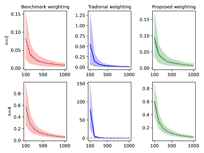
Figure 1: GMM loss at $B_{0}$ for different weighting schemes

Average, $10$%, and $90$% quantiles of the GMM loss $g_{T}(B)^{\prime}Wg_{T}(B)$ with all second-, to fourth-order moment conditions implied by mutually independent shocks, evaluated at $B=B_{0}$ using different weighting matrices with $2000$ simulations and sample sizes $T=100,...,1000$. The infeasible benchmark weighting in red uses $W=S^{-1}$, the traditional weighting in blue uses the weighting matrix equal to the inverse of the sample covariance matrix of the moment conditions, and the proposed weighting in green uses the the weighting matrix equal to the inverse of the the long-run covariance matrix based on Equation (13). The dotted gray line shows the expected value of the GMM objective function at $B_{0}$ with $W=S^{-1}$ which is equal to $K/T$ where $K$ denotes the number of moment conditions, see Han and Phillips, (2006) and Newey and Windmeijer, (2009).

The simulation results demonstrate that the traditional estimator for the asymptotically efficient weighting matrix is inadequate for approximating the true asymptotically efficient weighting matrix, particularly for large SVAR models. Specifically, in the SVAR model with four variables and small sample sizes, the average GMM loss using the traditional estimator for the asymptotically efficient weighting matrix substantially differs from the average GMM loss based on the true asymptotically efficient weighting matrix. In contrast, the proposed weighting scheme, which leverages the assumption of serially and mutually independent shocks, provides a close approximation to the infeasible asymptotically efficient weighting scheme, thus demonstrating its effectiveness.

5.2 Finite sample performance in medium-scaled SVAR models

The following section compares the performance of three asymptotically efficient estimators in the SVAR with four variables. The three estimators use all second-, third-, and fourth-order moment conditions implied by mutually independent shocks, including six covariance, $16$ coskewness, and $31$ cokurtosis conditions, as well as four additional moment conditions normalizing the variance of the shocks to one. The estimators analyzed are:

• GMM^∗: A one-step GMM estimator using the true but in practice unknown asymptotically efficient weighting matrix, which is equal to the inverse of the long-run covariance matrix.

• GMM: A two-step GMM estimator using an identity weighting matrix in the first step and the traditional estimator of the efficient weighting matrix in the second step, which is equal to the inverse of the sample covariance matrix of the moment conditions, assuming serially uncorrelated moment conditions or equivalently serially independent shocks.

• CSUE: The two-step continuous scale updating estimator using an identity weighting matrix in the first step and the proposed estimator of the efficient weighting matrix in the second step, which is equal to the inverse of the estimated long-run covariance matrix based on Equation (13), leveraging the assumption of serially and mutually independent shocks.

The first estimator GMM^∗ is the asymptotically efficient but infeasible estimator and serves as a benchmark. The second estimator GMM represents the standard implementation of a GMM estimator. The third estimator CSUE is the proposed GMM implementation tailored to address the SVAR specific GMM issues related to the difficulty of estimating the long-run covariance matrix and the small sample scaling bias.

Table 3 reports the mean, $10$% quantile, and $90$% quantile of the variance of the first innovation, i.e. the mean and quantiles of $v_{m}:=\frac{1}{T}\sum_{t=1}^{T}e(\hat{B})_{1t}^{2}$ for $m=1,...,2000$ simulations. The variance of the innovation is normalized to one by the unit variance moment conditions $\frac{1}{T}\sum_{t=1}^{T}e(B)_{1t}^{2}-1=0$ used by all three estimators. The infeasible, asymptotically efficient estimator, $\text{GMM}^{*}$, exhibits a downward variance scaling bias. Specifically, the mean of the variance of the first innovation is $0.88$, and even the upper $90$% quantile is $0.93$ and thus below the normalizing unit variance moment condition. This finding aligns with Proposition 1, which shows that the noise term of the asymptotically efficient estimator leads to a small sample bias towards solutions with a variance below the normalizing unit variance condition. Moreover, the innovations corresponding to the traditional GMM estimator exhibit a variance bias in the opposite direction, indicating that it poorly approximates the asymptotically efficient estimator. In contrast, the innovations corresponding to the proposed CSUE estimator are centered around the unit variance condition, demonstrating the effectiveness of the variance scaling correction.

Table 3: Mean and quantiles of the variance of the estimated structural shocks.

	$T=300$			$T=800$
	mean	Q$10$%	Q$90$%	mean	Q$10$%	Q$90$%
$\text{GMM}^{*}$	$0.88$	$0.82$	$0.93$	$0.93$	$0.9$	$0.97$
GMM	$1.04$	$0.76$	$1.3$	$1.08$	$0.99$	$1.17$
CSUE	$1.01$	$0.96$	$1.06$	$1.0$	$0.97$	$1.03$

Note: The table shows the mean, $10$% quantile, and $90$% quantile of the variance of the first innovation, i.e. the mean and quantiles of $v_{m}:=\frac{1}{T}\sum_{t=1}^{T}e(\hat{B})_{1t}^{2}$ for $m=1,...,2000$ simulations.

Table 4 displays the mean, median, interquartile range (IQR), and standard deviation (SD) of the estimates for three representative elements of $B_{0}$ in Equation (33): the lower left element $\hat{B}_{41}$, the first diagonal element $\hat{B}_{11}$, and the upper right element $\hat{B}_{14}$. The proposed CSUE exhibits the smallest mean bias, median bias, interquartile range, and standard deviation, and outperforms the alternative estimators. It is worth noting that the bias of the diagonal and lower triangular element is related to the variance scaling bias reported in Table 3. This also explains why the upper triangular element is unbiased, as it is zero and hence not affected by the variance scaling bias.

Table 4: Mean, median, interquartile range, and standard deviation of three representative estimates.

	$T=300$
	estimator $\hat{B}_{41}$ for $B_{41}=5$				estimator $\hat{B}_{11}$ for $B_{11}=10$				estimator $\hat{B}_{14}$ for $B_{14}=0$
	mean	med	IQR	sd	mean	med	IQR	sd	mean	med	IQR	sd
$\text{GMM}^{*}$	$5.24$	$5.3$	$1.9$	$2.55$	$10.45$	$10.53$	$1.61$	$1.86$	$-0.02$	$-0.03$	$1.41$	$1.49$
GMM	$4.55$	$4.63$	$2.68$	$8.17$	$9.26$	$9.32$	$2.17$	$6.23$	$0.03$	$-0.01$	$2.07$	$4.91$
CSUE	$4.89$	$4.93$	$1.73$	$1.99$	$9.8$	$9.89$	$1.42$	$1.32$	$0.02$	$-0.01$	$1.32$	$1.25$
	$T=800$
	estimator $\hat{B}_{41}$ for $B_{41}=5$				estimator $\hat{B}_{11}$ for $B_{11}=10$				estimator $\hat{B}_{14}$ for $B_{14}=0$
	mean	med	IQR	sd	mean	med	IQR	sd	mean	med	IQR	sd
$\text{GMM}^{*}$	$5.13$	$5.12$	$1.1$	$0.7$	$10.28$	$10.29$	$0.92$	$0.54$	$-0.01$	$-0.01$	$0.82$	$0.42$
GMM	$4.73$	$4.73$	$1.19$	$1.01$	$9.55$	$9.54$	$1.03$	$0.78$	$-0.01$	$-0.02$	$0.96$	$0.58$
CSUE	$4.96$	$4.94$	$1.02$	$0.58$	$9.94$	$9.95$	$0.82$	$0.39$	$-0.0$	$-0.01$	$0.78$	$0.36$

Note: The table shows the mean, median, interquartile range (IQR), and standard deviation (sd) of the lower left element $\hat{B}_{41}$, the first diagonal element $\hat{B}_{11}$, and the upper right element $\hat{B}_{14}$ in Equation (33) across $2000$ simulations.

The second part of the finite sample analysis focuses on the impact of the weighting scheme and the estimation of the asymptotic variance on the coverage of confidence bands and rejection frequencies for various Wald tests. The construction of these bands and tests requires estimates of $S$ and $G$, required for the asymptotic variance in Equation (8). To this end, I present results in two sets of columns: SMI and SI. The SMI columns estimate $S$ and $G$ by assuming serially and mutually independent shocks, as proposed in Section 3 and the SI columns follow the traditional approach and estimate $S$ and $G$ by only assuming serially independent shocks, which is equivalent to assuming serially uncorrelated moment conditions.

Table 5 presents the coverage of $90$% confidence bands for the three representative elements of the estimators. Notably, the traditional approach based on serially uncorrelated moment conditions exhibits a substantial shortfall in achieving the $90$% coverage level, with the coverage rate barely approaching $60$% even for the large sample case with $T=800$ observations. In contrast, the coverage rates of the bands of the CSUE, which are calculated based on the assumption of serially and mutually independent shocks, are substantially better and close to the $90$% level. The infeasible $\text{GMM}^{*}$ estimator does not rely on estimates of the asymptotically efficient weighting matrix and provides further insight into the effect of the estimated $S$ and $G$ matrices on the estimated asymptotic variance and its impact on the coverage of the confidence bands. The coverage of the $\text{GMM}^{*}$ bands using only serially independent shocks are worse than coverage rates using serially and mutually independent shocks. However, the $\text{GMM}^{*}$ bands using only serially independent shocks substantially improve compared to the GMM bands which are also constructed under the assumption of serially independent shocks, indicating that a large part of the poor coverage rate of the traditional GMM estimator can be attributed to unprecise estimates of the $B_{0}$ matrix.

Table 5: Coverage of three representative estimates.

	$T=300$						$T=800$
	$B_{41}$		$B_{11}$		$B_{14}$		$B_{41}$		$B_{11}$		$B_{14}$
	SMI	SI	SMI	SI	SMI	SI	SMI	SI	SMI	SI	SMI	SI
$\text{GMM}^{*}$	$85.0$	$71.0$	$81.0$	$74.0$	$86.0$	$73.0$	$87.0$	$81.0$	$83.0$	$81.0$	$88.0$	$82.0$
GMM	/	$29.0$	/	$32.0$	/	$30.0$	/	$55.0$	/	$54.0$	/	$55.0$
CSUE	$84.0$	/	$86.0$	/	$85.0$	/	$88.0$	/	$88.0$	/	$88.0$	/

Note: The table shows the coverage of the $90$% intervals in percent for the lower diagonal element $B_{41}$, the diagonal element $B_{11}$, and the upper diagonal element $B_{14}$ in Equation (33) across $2000$ simulations. The intervals depend on the estimated asymptotic variance $\hat{M}\hat{S}\hat{M}$ with $\hat{M}=(\hat{G}^{\prime}\hat{S}^{-1}\hat{G})^{-1}\hat{G}^{\prime}W$ where $W$ is equal to the weighing matrix used by the corresponding estimator and $\hat{S}$ and $\hat{G}$ are estimates of $S$ and $G$ depending on the label of a given column. For columns labeled SMI, elements of $\hat{S}$ and $\hat{G}$ are calculated based on Equation (13) and (16). For columns labeled SMI, the matrix $\hat{S}$ is calculated as the the sample covariance matrix of the moment conditions and the elements of $\hat{G}$ are calculated based on Equation (15).

Table 6 reports the rejection rates at the $10$% level for three different Wald tests. The first test examines the joint null hypothesis $B=B_{0}$, the second tests the joint null hypothesis that the SVAR is recursive, meaning the upper triangular of $B_{0}$ contains only zeros, and the last test examines if the $B_{14}$ element is equal to zero. The table illustrates that the test performance decreases with the number of jointly tested coefficients. Moreover, the rejection rates of the GMM estimator are again far from the $10$% level, even in the large sample with $T=800$ observations. In contrast, the proposed CSUE estimator displays substantially improved performance, although it still rejects too often in small samples when multiple coefficients are jointly tested.

Table 6: Rejection rates at $\alpha=10$% for different Wald tests.

	$T=300$						$T=800$
	$H_{0}$$:$$B$$=$$B_{0}$		$H_{0}$$:$$B$$=$$B_{rec}$		$H_{0}$$:$$B_{14}$$=$$0$		$H_{0}$$:$$B$$=$$B_{0}$		$H_{0}$$:$$B$$=$$B_{rec}$		$H_{0}$$:$$B_{14}$$=$$0$
	SMI	SI	SMI	SI	SMI	SI	SMI	SI	SMI	SI	SMI	SI
$\text{GMM}^{*}$	$42.0$	$77.0$	$25.0$	$66.0$	$14.0$	$27.0$	$32.0$	$44.0$	$19.0$	$40.0$	$12.0$	$18.0$
GMM	/	$100.0$	/	$100.0$	/	$70.0$	/	$99.0$	/	$90.0$	/	$45.0$
CSUE	$34.0$	/	$28.0$	/	$15.0$	/	$22.0$	/	$19.0$	/	$12.0$	/

Note: The table shows the rejection rates in percent at $\alpha=10$% for three different Wald tests. The first test with $H_{0}:B=B_{0}$ tests the null hypothesis that $B$ is equal to $B_{0}$ from Equation (33), the second test with $H_{0}:B=B_{rec}$ tests the null hypothesis of a recursive SVAR, and the third test with $H_{0}:B_{14}=0$ tests the null hypothesis that the impact of the fourth shock on the first variable is zero. All three null hypotheses are correct. The tests depend on the estimated asymptotic variance $\hat{M}\hat{S}\hat{M}$ with $\hat{M}=(\hat{G}^{\prime}\hat{S}^{-1}\hat{G})^{-1}\hat{G}^{\prime}W$ where $W$ is equal to the weighing matrix used by the corresponding estimator and $\hat{S}$ and $\hat{G}$ are estimates of $S$ and $G$ depending on the label of a given column. For columns labeled SMI, elements of $\hat{S}$ and $\hat{G}$ are calculated based on Equation (13) and (16). For columns labeled SMI, the matrix $\hat{S}$ is calculated as the the sample covariance matrix of the moment conditions and the elements of $\hat{G}$ are calculated based on Equation (15).

Lastly, Table 7 analyzes the impact of the different approaches on the power of a single coefficient Wald test. The table shows the rejection rates at the $10$% level for the Wald test with $H_{0}:B_{41}=b$ and $b=2,...,8$ where the true value of the $B_{41}$ element is five. Again, the GMM estimator rejects the correct null hypothesis $B_{41}=5$ too often with rejection in more than $60$% of the simulations. Moreover, the rejection rates increase only by around $30$ percentage points for the tests with $H_{0}:B_{41}=2$ and $H_{0}:B_{41}=8$ in the small sample. In contrast, the proposed CSUE estimator exhibits much better performance, with the rejection rate for the correct null hypothesis $B_{41}=5$ being closer to the $10$% level. Additionally, the rejection rate increases more strongly, by around $65$ percentage points, for the tests with $H_{0}:B_{41}=2$ and $H_{0}:B_{41}=8$ in the small sample.

Table 7: Rejection rates at $\alpha=10$% for the Wald test with $H_{0}:B_{41}=b$ and $b=2,...,8$.

	$T=300$
	SMI							SI
b	$2$	$3$	$4$	$5$	$6$	$7$	$8$	$2$	$3$	$4$	$5$	$6$	$7$	$8$
$\text{GMM}^{*}$	$77.0$	$55.0$	$30.0$	$15.0$	$18.0$	$40.0$	$66.0$	$87.0$	$70.0$	$46.0$	$29.0$	$33.0$	$56.0$	$79.0$
GMM	/	/	/	/	/	/	/	$89.0$	$80.0$	$72.0$	$71.0$	$78.0$	$86.0$	$92.0$
CSUE	$79.0$	$53.0$	$27.0$	$16.0$	$29.0$	$58.0$	$83.0$	/	/	/	/	/	/	/
	$T=800$
	SMI							SI
b	$2$	$3$	$4$	$5$	$6$	$7$	$8$	$2$	$3$	$4$	$5$	$6$	$7$	$8$
$\text{GMM}^{*}$	$98.0$	$86.0$	$45.0$	$13.0$	$33.0$	$78.0$	$97.0$	$99.0$	$89.0$	$52.0$	$19.0$	$40.0$	$82.0$	$98.0$
GMM	/	/	/	/	/	/	/	$98.0$	$87.0$	$58.0$	$45.0$	$74.0$	$94.0$	$100.0$
CSUE	$99.0$	$85.0$	$40.0$	$12.0$	$44.0$	$87.0$	$100.0$	/	/	/	/	/	/	/

Note: The table shows the rejection rates in percent at $\alpha=10$% for the Wald test with $H_{0}:B_{41}=b$ and $b=2,...,8$. The true value of $B_{41}$ is five. The tests depend on the estimated asymptotic variance $\hat{M}\hat{S}\hat{M}$ with $\hat{M}=(\hat{G}^{\prime}\hat{S}^{-1}\hat{G})^{-1}\hat{G}^{\prime}W$ where $W$ is equal to the weighing matrix used by the corresponding estimator and $\hat{S}$ and $\hat{G}$ are estimates of $S$ and $G$ depending on the label of a given column. For columns labeled SMI, elements of $\hat{S}$ and $\hat{G}$ are calculated based on Equation (13) and (16). For columns labeled SMI, the matrix $\hat{S}$ is calculated as the the sample covariance matrix of the moment conditions and the elements of $\hat{G}$ are calculated based on Equation (15).

5.3 Additional simulations

Appendix B.1 presents additional results for various asymptotically efficient moment-based estimators in the simulation discussed in the previous section. The simulations demonstrate that adding the scaling term proposed in Section 4 to the infeasible $\text{GMM}^{*}$ estimator using the true but in practice unknown efficient weighting matrix yields the infeasible $\text{CSUE}^{*}$, which successfully eliminates the scaling bias and performs similar to the proposed CSUE analyzed in the previous section that leverages the assumption of mutually and serially independent shocks to estimate the weighting matrix. Moreover, the continuous updating estimator that uses the assumption of mutually and serially independent shocks to estimate the weighting matrix performs similarly to the proposed CSUE estimator, while the continuous updating estimator that only uses the assumption of serially independent shocks performs worse than the two-step GMM estimator analyzed in the main text. Furthermore, adding the scaling term to the traditional two-step GMM estimator that does not use the assumption of mutually independent shocks to estimate the weighting matrix is not enough to eliminate the variance scaling bias, but it leads to less volatile estimates.

Appendix B.2, B.3, and B.4 present results for the estimators examined in the previous sections in SVAR models with structural shocks generated from different distributions, including a skewed normal distribution, a t-distribution, and a truncated normal distribution. The findings are consistent with those in the previous section. Specifically, the infeasible asymptotically efficient GMM estimator exhibits a scaling bias towards innovations with variances smaller than one and the CSUE eliminates the bias by including a continuously updated scaling term. Moreover, the CSUE outperforms the GMM estimator in terms of bias and volatility, highlighting the importance of utilizing the assumption of serially and mutually independent shocks to estimate the efficient weighting matrix and of incorporating the scaling term to avoid the scaling bias. Lastly, using the assumption of serially and mutually independent shocks to estimate the asymptotic variance of the estimator leads to a significant improvement in the rejection rates of the considered Wald tests.

While the focus of this study is on estimating the simulations interaction $u_{t}=B_{0}\varepsilon_{t}$, applications of SVAR models typically also involve estimating a VAR with a lag structure, $y_{t}=\sum_{p=1}^{P}A_{p}y_{t-p}+u_{t}$. This can be done in a two-step approach: first, the VAR is estimated, and then, in the second step, the simultaneous interaction is estimated using the reduced form shocks obtained from the initial estimation. Employing such a two-step approach affects the asymptotic variance of the GMM estimator in Equation (8), see Appendix Subsection 5.2 in Gouriéroux et al., (2020). In Appendix B.5, I present simulations for an SVAR with lags estimated using the two-step approach. The results reaffirm the core findings presented in this section. Specifically, even when employing the two-step approach, the $\text{GMM}^{*}$ estimator continues to display the same scaling bias and the CSUE eliminates the bias. Moreover, the CSUE outperforms the GMM estimator and using the assumption of serially and mutually independent shocks to estimate the asymptotic variance leads to a notable enhancement in the rejection rates of the Wald tests under consideration.

Finally, achieving more accurate estimates of the efficient weighting matrix and asymptotic variance hinges upon assuming mutually independent shocks. However, a commonly voiced concern regarding this assumption is that macroeconomic shocks may be influenced by a shared volatility process, as discussed in Montiel Olea et al., (2022) and others. In this scenario, estimates of $S$ relying on the assumption of mutually independent shocks are no longer consistent and may lead to inefficient weighting and distorted inference. Appendix B.6 analyzes the impact of a common volatility process on the estimators considered in the previous section. First, the findings concerning the scaling bias and the superior performance of the CSUE to the GMM estimator in terms of bias and variance remain unaltered. Secondly, the rejection frequencies of the considered Wald test relying on estimates of asymptotic variance under the assumption of mutually independent shocks deteriorates, however, they still outperform the Wald tests not relying on estimates of asymptotic variance by a large margin.

6 Conclusion

This study investigates the small sample performance of asymptotically efficient SVAR-GMM estimators based on higher-order moment conditions derived from independent shocks. The simulations reveal that standard implementations of GMM estimators lead to a poor small sample performance. I propose two measures that significantly improve estimator performance. First, I propose the contentious scale updating estimator, which adds a continuously updated scaling term to the weighting matrix, thereby avoiding the small sample variance scaling bias of the asymptotically efficient GMM estimator. Second, I simplify the estimation of the long-run covariance matrix of the moment conditions by leveraging the assumption of serially and mutually independent shocks. This leads to more precise estimates of the asymptotically efficient weighting matrix and of the asymptotic variance of the estimator. The Monte Carlo simulation demonstrates that these measures lead to substantial improvements in the finite sample performance of the estimator.

Appendix A Proof

The following lemma calculates the specific noise term of the SVAR-GMM estimator at $\tilde{B}=BD$ with a scaling matrix $D=diag(d_{1},...,d_{n})$.

Lemma 1.

For moment conditions $f(B,u_{t})=[f_{m_{1}}(B,u_{t}),...,f_{m_{K}}(B,u_{t})]^{\prime}$ with $f_{m_{k}}(B,u_{t}):=\prod_{i=1}^{n}e(B)_{i,t}^{m_{k,i}}-c(m_{k}))$ and serially independent shocks, the noise term $trace(WS(BD))/T$ is equal to

$$\frac{1}{T}\sum_{k=1}^{k}\frac{1}{\prod_{i=1}^{n}d_{i}^{2m_{k,i}}}\left(WS(\tilde{B})\right)_{kk}$$

$$+\frac{2}{T}\sum_{k=1}^{k}c(m_{k})\frac{1-\prod_{i=1}^{n}d_{i}^{m_{k,i}}}{\prod_{i=1}^{n}d_{i}^{2m_{k,i}}}E\left[f_{m_{k}}(\tilde{B},u_{t})\right]W_{kk}$$ (35)

$$+\frac{1}{T}\sum_{k=1}^{k}c(m_{k})\left(\frac{1}{\prod_{i=1}^{n}d_{i}^{m_{k,i}}}-1\right)^{2}W_{kk},$$

with $\tilde{B}:=BD$ for a scaling matrix $D=diag(d_{1},...,d_{n})$ and where $W_{kk}$ and $\left(WS(\tilde{B})\right)_{kk}$ denote the $k$-th diagonal element of $W$ and $\left(WS(\tilde{B})\right)$ respectively.

Proof of Lemma 1.

For a moment condition $E\left[f_{m}(B,u_{t})\right]$ and a diagonal scaling matrix $D=diag(d_{1},...,d_{n})$ it holds that

$$f_{m}(BD,u_{t}) =\prod_{i=1}^{n}e(BD)_{i,t}^{m_{i}}-c(m)$$ (36)

$$=\prod_{i=1}^{n}\frac{1}{d_{i}^{m_{i}}}e(B)_{i,t}^{m_{i}}-c(m)$$ (37)

$$=\prod_{i=1}^{n}\frac{1}{d_{i}^{m_{i}}}e(B)_{i,t}^{m_{i}}-c(m)+c(m)\left(\prod_{i=1}^{n}\frac{1}{d_{i}^{m_{i}}}-1\right)$$ (38)

$$=\frac{1}{d_{1}^{m_{1}}....d_{n}^{m_{n}}}f_{m}(B,u_{t})+c(m)\left(\frac{1}{d_{1}^{m_{1}}....d_{n}^{m_{n}}}-1\right).$$ (39)

Therefore, the vector of all moment conditions $f(B,u_{t})=[f_{m_{1}}(B,u_{t}),...,f_{m_{K}}(B,u_{t})]^{\prime}$ with $f_{m_{k}}(B,u_{t}):=\prod_{i=1}^{n}e(B)_{i,t}^{m_{k,i}}-c(m_{k}))$ can be written as

$$f(BD,u_{t})=\tilde{D}f(B,u_{t})+(\tilde{D}-I)C,$$ (40)

with $C:=[c(m_{1}),...,c(m_{K})]^{\prime}$ and $\tilde{D}=diag(\frac{1}{\prod_{i=1}^{n}d_{i}^{m_{1,i}}},...,\frac{1}{\prod_{i=1}^{n}d_{i}^{m_{K,i}}})$.

The variance covariance matrix $S(BD)$ is thus equal to

$$S(BD)=E \left[f(BD,u_{t})f(BD,u_{t})^{\prime}\right]$$ (41)

$$=E \left[\left(\tilde{D}f(B,u_{t})+(\tilde{D}-I)c\right)\left(\tilde{D}f(B,u_{t})+(\tilde{D}-I)c\right)^{\prime}\right]$$ (42)

$$=E \left[\left(\tilde{D}f(B,u_{t})+(\tilde{D}-I)C\right)\left(f(B,u_{t})^{\prime}\tilde{D}^{\prime}+C^{\prime}(\tilde{D}-I)^{\prime}\right)\right]$$ (43)

$$=E [\tilde{D}f(B,u_{t})f(B,u_{t})^{\prime}\tilde{D}$$ (44)

$$+\tilde{D}f(B,u_{t})C^{\prime}(\tilde{D}-I)$$

$$+(\tilde{D}-I)Cf(B,u_{t})^{\prime}\tilde{D}$$

$$+(\tilde{D}-I)CC^{\prime}(\tilde{D}-I)]$$

$$=\tilde{D} S(B)\tilde{D}+\tilde{D}E\left[f(B,u_{t})\right]C^{\prime}(\tilde{D}-I)$$ (45)

$$+ (\tilde{D}-I)CE\left[f(B,u_{t})\right]^{\prime}\tilde{D}+(\tilde{D}-I)CC^{\prime}(\tilde{D}-I).$$

Moreover, with diagonal matrices $\tilde{D}$ and $(\tilde{D}-I))$ and for a weighting matrix $W$ it holds that

$$trace(W\tilde{D}S(B)\tilde{D}) =\sum_{k=1}^{K}\left(\frac{1}{\prod_{i=1}^{n}d_{i}^{m_{k,i}}}\right)^{2}\left(WS(B)\right)_{kk}$$ (46)

and

$$trace(W\tilde{D}E\left[f(B,u_{t})\right]C^{\prime}(\tilde{D}-I)) =trace(WCE\left[f(B,u_{t})\right]^{\prime}\tilde{D}(\tilde{D}-I))$$ (47)

$$=\sum_{k=1}^{K}(WCE\left[f(B,u_{t})\right]^{\prime})_{kk}(\tilde{D}(\tilde{D}-I)))_{kk}$$ (48)

$$=\sum_{k=1}^{K}\frac{1}{\prod_{i=1}^{n}d_{i}^{m_{k,i}}}\left(\frac{1}{\prod_{i=1}^{n}d_{i}^{m_{k,i}}}-1\right)c(m_{k})E\left[f_{m_{k}}(B,u_{t})\right]W_{kk}$$ (49)

and

$$trace(W(\tilde{D}-I)CE\left[f(B,u_{t})\right]^{\prime}\tilde{D}) =trace(WE\left[f(B,u_{t})\right]C^{\prime}(\tilde{D}-I)\tilde{D})$$ (50)

$$=\sum_{k=1}^{K}(WE\left[f(B,u_{t})\right]C^{\prime})_{kk}((\tilde{D}-I)\tilde{D})_{kk}$$ (51)

$$=\sum_{k=1}^{K}\frac{1}{\prod_{i=1}^{n}d_{i}^{m_{k,i}}}\left(\frac{1}{\prod_{i=1}^{n}d_{i}^{m_{k,i}}}-1\right)C(m_{k})E\left[f_{m_{k}}(B,u_{t})\right]W_{kk}$$ (52)

and

$$trace(W(\tilde{D}-I)CC^{\prime}(\tilde{D}-I)) =trace(WCC^{\prime}(\tilde{D}-I)(\tilde{D}-I))$$ (53)

$$=\sum_{k=1}^{K}(WCC^{\prime})_{kk}((\tilde{D}-I)(\tilde{D}-I))_{kk}$$ (54)

$$=\sum_{k=1}^{K}\left(\frac{1}{\prod_{i=1}^{n}d_{i}^{m_{k,i}}}-1\right)^{2}c(m_{k})W_{kk}.$$ (55)

Therefore,

$$trace(WS(BD))= trace(W\tilde{D}S(B)\tilde{D})$$ (56)

$$+trace(W\tilde{D}E\left[f(B,u_{t})\right]C^{\prime}(\tilde{D}-I))$$ (57)

$$+trace(W(\tilde{D}-I)CE\left[f(B,u_{t})\right]^{\prime}\tilde{D})$$ (58)

$$+trace(W(\tilde{D}-I)CC^{\prime}(\tilde{D}-I))$$ (59)

$$= \sum_{k=1}^{K}\left(\frac{1}{\prod_{i=1}^{n}d_{i}^{m_{k,i}}}\right)^{2}\left(WS(B)\right)_{kk}$$ (60)

$$+2\sum_{k=1}^{K}\frac{1}{\prod_{i=1}^{n}d_{i}^{m_{k,i}}}\left(\frac{1}{\prod_{i=1}^{n}d_{i}^{m_{k,i}}}-1\right)W_{kk}c(m_{k})E\left[f_{m_{k}}(B,u_{t})\right]$$ (61)

$$+\sum_{k=1}^{K}\left(\frac{1}{\prod_{i=1}^{n}d_{i}^{m_{k,i}}}-1\right)^{2}W_{kk}c(m_{k}).$$ (62)

∎

Appendix B Additional Monte Carlo simulations

B.1 Results for additional estimators

This section contains results for additional estimators in the Monte Carlo simulation presented in Section 5. All considered estimators are implementations of asymptotically efficient GMM estimators using all second to fourth order moment conditions implied by mutually independent shocks with unit variance. The estimators analyzed are:

• $\text{GMM}_{\text{SMI}}$: Two-step GMM estimator using an identity weighting matrix in the first step and the proposed estimator of the efficient weighting matrix in the second step, which is equal to the inverse of the estimated long-run covariance matrix based on Equation (13), leveraging the assumption of serially and mutually independent shocks.

• $\text{CSUE}_{\text{SMI}}$: Two-step continuous scale updating estimator using an identity weighting matrix in the first step and the proposed estimator of the efficient weighting matrix in the second step, which is equal to the inverse of the estimated long-run covariance matrix based on Equation (13), leveraging the assumption of serially and mutually independent shocks.

• $\text{CUE}_{\text{SMI}}$: Continuous updating estimator where the weighting matrix is continuously updated and estimated using the proposed estimator of the efficient weighting matrix, which is equal to the inverse of the estimated long-run covariance matrix based on Equation (13), leveraging the assumption of serially and mutually independent shocks.

• $\text{GMM}_{\text{SI}}$: Two-step GMM estimator using an identity weighting matrix in the first step and the traditional estimator of the efficient weighting matrix in the second step, which is equal to the inverse of the sample covariance matrix of the moment conditions, assuming serially uncorrelated moment conditions or equivalently serially independent shocks.

• $\text{CSUE}_{\text{SI}}$: Two-step continuous scale updating estimator using an identity weighting matrix in the first step and the traditional estimator of the efficient weighting matrix in the second step, which is equal to the inverse of the sample covariance matrix of the moment conditions, assuming serially uncorrelated moment conditions or equivalently serially independent shocks.

• $\text{CUE}_{\text{SI}}$: Continuous updating estimator where the weighting matrix is continuously updated and estimated using the traditional estimator of the efficient weighting matrix, which is equal to the inverse of the sample covariance matrix of the moment conditions, assuming serially uncorrelated moment conditions or equivalently serially independent shocks.

• GMM^∗: One-step GMM estimator using the true but in practice unknown asymptotically efficient weighting matrix.

• CSUE^∗: One-step continuous scale updating estimator using the true but in practice unknown asymptotically efficient weighting matrix.

Table 8: Mean and quantiles of the variance of the estimated structural shocks.

	$T=300$			$T=800$
	mean	Q$10$%	Q$90$%	mean	Q$10$%	Q$90$%
$\text{GMM}_{\text{SMI}}$	$0.87$	$0.8$	$0.94$	$0.93$	$0.89$	$0.97$
$\text{CSUE}_{\text{SMI}}$	$1.01$	$0.96$	$1.06$	$1.0$	$0.97$	$1.03$
$\text{CUE}_{\text{SMI}}$	$1.01$	$0.97$	$1.07$	$1.01$	$0.98$	$1.04$
$\text{GMM}_{\text{SI}}$	$1.04$	$0.76$	$1.3$	$1.08$	$0.99$	$1.17$
$\text{CSUE}_{\text{SI}}$	$1.37$	$1.15$	$1.64$	$1.16$	$1.07$	$1.26$
$\text{CUE}_{\text{SI}}$	$1.42$	$1.21$	$1.64$	$1.19$	$1.09$	$1.31$
$\text{GMM}^{*}$	$0.88$	$0.82$	$0.93$	$0.93$	$0.9$	$0.97$
$\text{CSUE}^{*}$	$1.0$	$0.96$	$1.05$	$1.0$	$0.97$	$1.03$

Note: The table shows the mean, $10$% quantile, and $90$% quantile of the variance of the first innovation, i.e. the mean and quantiles of $v_{m}:=\frac{1}{T}\sum_{t=1}^{T}e(\hat{B})_{1t}^{2}$ for $m=1,...,2000$ simulations.

Table 9: Mean, median, interquartile range, and standard deviation of three representative estimates.

	$T=300$
	estimator $\hat{B}_{41}$ for $B_{41}=5$				estimator $\hat{B}_{11}$ for $B_{11}=10$				estimator $\hat{B}_{14}$ for $B_{14}=0$
	mean	med	IQ	sd	mean	med	IQ	sd	mean	med	IQ	sd
$\text{GMM}_{\text{SMI}}$	$5.23$	$5.27$	$1.88$	$2.7$	$10.5$	$10.54$	$1.59$	$1.94$	$0.03$	$-0.01$	$1.41$	$1.55$
$\text{CSUE}_{\text{SMI}}$	$4.89$	$4.93$	$1.73$	$1.99$	$9.8$	$9.89$	$1.42$	$1.32$	$0.02$	$-0.01$	$1.32$	$1.25$
$\text{CUE}_{\text{SMI}}$	$4.87$	$4.93$	$1.75$	$2.02$	$9.73$	$9.85$	$1.4$	$1.41$	$-0.0$	$-0.02$	$1.29$	$1.22$
$\text{GMM}_{\text{SI}}$	$4.55$	$4.63$	$2.68$	$8.17$	$9.26$	$9.32$	$2.17$	$6.23$	$0.03$	$-0.01$	$2.07$	$4.91$
$\text{CSUE}_{\text{SI}}$	$4.2$	$4.26$	$1.63$	$2.46$	$8.46$	$8.48$	$1.49$	$3.65$	$0.03$	$0.01$	$1.23$	$1.18$
$\text{CUE}_{\text{SI}}$	$3.61$	$3.76$	$3.75$	$12.19$	$7.16$	$7.76$	$3.21$	$15.33$	$-0.05$	$-0.05$	$2.55$	$5.6$
$\text{GMM}^{*}$	$5.24$	$5.3$	$1.9$	$2.55$	$10.45$	$10.53$	$1.61$	$1.86$	$-0.02$	$-0.03$	$1.41$	$1.49$
$\text{CSUE}^{*}$	$4.91$	$4.98$	$1.84$	$2.22$	$9.77$	$9.88$	$1.43$	$1.48$	$-0.01$	$-0.03$	$1.36$	$1.38$
	$T=800$
	estimator $\hat{B}_{41}$ for $B_{41}=5$				estimator $\hat{B}_{11}$ for $B_{11}=10$				estimator $\hat{B}_{14}$ for $B_{14}=0$
	mean	med	IQ	sd	mean	med	IQ	sd	mean	med	IQ	sd
$\text{GMM}_{\text{SMI}}$	$5.13$	$5.12$	$1.07$	$0.65$	$10.29$	$10.29$	$0.89$	$0.53$	$-0.01$	$-0.02$	$0.81$	$0.39$
$\text{CSUE}_{\text{SMI}}$	$4.96$	$4.94$	$1.02$	$0.58$	$9.94$	$9.95$	$0.82$	$0.39$	$-0.0$	$-0.01$	$0.78$	$0.36$
$\text{CUE}_{\text{SMI}}$	$4.95$	$4.94$	$1.03$	$0.58$	$9.92$	$9.94$	$0.81$	$0.39$	$-0.0$	$-0.01$	$0.79$	$0.36$
$\text{GMM}_{\text{SI}}$	$4.73$	$4.73$	$1.19$	$1.01$	$9.55$	$9.54$	$1.03$	$0.78$	$-0.01$	$-0.02$	$0.96$	$0.58$
$\text{CSUE}_{\text{SI}}$	$4.59$	$4.6$	$1.05$	$0.84$	$9.23$	$9.24$	$0.9$	$1.03$	$0.0$	$0.01$	$0.82$	$0.4$
$\text{CUE}_{\text{SI}}$	$4.55$	$4.51$	$1.44$	$2.26$	$8.98$	$9.13$	$1.14$	$2.51$	$-0.05$	$-0.04$	$1.05$	$1.2$
$\text{GMM}^{*}$	$5.13$	$5.12$	$1.1$	$0.7$	$10.28$	$10.29$	$0.92$	$0.54$	$-0.01$	$-0.01$	$0.82$	$0.42$
$\text{CSUE}^{*}$	$4.97$	$4.95$	$1.06$	$0.65$	$9.93$	$9.95$	$0.87$	$0.42$	$-0.0$	$-0.0$	$0.82$	$0.4$

Note: The table shows the mean, median, interquartile range (IQR), and standard deviation (sd) of the lower left element $\hat{B}_{41}$, the first diagonal element $\hat{B}_{11}$, and the upper right element $\hat{B}_{14}$ in Equation (33) across $2000$ simulations.

Table 10: Coverage of three representative estimates.

	$T=300$						$T=800$
	$B_{41}$		$B_{11}$		$B_{14}$		$B_{41}$		$B_{11}$		$B_{14}$
	SMI	SI	SMI	SI	SMI	SI	SMI	SI	SMI	SI	SMI	SI
$\text{GMM}_{\text{SMI}}$	$84.0$	/	$79.0$	/	$85.0$	/	$87.0$	/	$82.0$	/	$88.0$	/
$\text{CSUE}_{\text{SMI}}$	$84.0$	/	$86.0$	/	$85.0$	/	$88.0$	/	$88.0$	/	$88.0$	/
$\text{CUE}_{\text{SMI}}$	$84.0$	/	$86.0$	/	$84.0$	/	$88.0$	/	$88.0$	/	$88.0$	/
$\text{GMM}_{\text{SI}}$	/	$29.0$	/	$32.0$	/	$30.0$	/	$55.0$	/	$54.0$	/	$55.0$
$\text{CSUE}_{\text{SI}}$	/	$36.0$	/	$22.0$	/	$42.0$	/	$56.0$	/	$41.0$	/	$61.0$
$\text{CUE}_{\text{MI}}$	/	$17.0$	/	$16.0$	/	$22.0$	/	$42.0$	/	$35.0$	/	$50.0$
$\text{GMM}^{*}$	$85.0$	$71.0$	$81.0$	$74.0$	$86.0$	$73.0$	$87.0$	$81.0$	$83.0$	$81.0$	$88.0$	$82.0$
$\text{CSUE}^{*}$	$85.0$	$71.0$	$87.0$	$80.0$	$85.0$	$71.0$	$88.0$	$81.0$	$88.0$	$86.0$	$88.0$	$82.0$

Note: The table shows the coverage of the $90$% intervals in percent for the lower diagonal element $B_{41}$, the diagonal element $B_{11}$, and the upper diagonal element $B_{14}$ in Equation (33) across $2000$ simulations. The intervals depend on the estimated asymptotic variance $\hat{M}\hat{S}\hat{M}$ with $\hat{M}=(\hat{G}^{\prime}\hat{S}^{-1}\hat{G})^{-1}\hat{G}^{\prime}W$ where $W$ is equal to the weighing matrix used by the corresponding estimator and $\hat{S}$ and $\hat{G}$ are estimates of $S$ and $G$ depending on the label of a given column. For columns labeled SMI, elements of $\hat{S}$ and $\hat{G}$ are calculated based on Equation (13) and (16). For columns labeled SMI, the matrix $\hat{S}$ is calculated as the the sample covariance matrix of the moment conditions and the elements of $\hat{G}$ are calculated based on Equation (15).

Table 11: Rejection rates at $\alpha=10$% for different Wald tests.

	$T=300$						$T=800$
	$H_{0}$$:$$B$$=$$B_{0}$		$H_{0}$$:$$B$$=$$B_{rec}$		$H_{0}$$:$$B_{14}$$=$$0$		$H_{0}$$:$$B$$=$$B_{0}$		$H_{0}$$:$$B$$=$$B_{rec}$		$H_{0}$$:$$B_{14}$$=$$0$
	SMI	SI	SMI	SI	SMI	SI	SMI	SI	SMI	SI	SMI	SI
$\text{GMM}_{\text{SMI}}$	$50.0$	/	$29.0$	/	$15.0$	/	$36.0$	/	$19.0$	/	$12.0$	/
$\text{CSUE}_{\text{SMI}}$	$34.0$	/	$28.0$	/	$15.0$	/	$22.0$	/	$19.0$	/	$12.0$	/
$\text{CUE}_{\text{SMI}}$	$33.0$	/	$30.0$	/	$16.0$	/	$21.0$	/	$20.0$	/	$12.0$	/
$\text{GMM}_{\text{SI}}$	/	$100.0$	/	$100.0$	/	$70.0$	/	$99.0$	/	$90.0$	/	$45.0$
$\text{CSUE}_{\text{SI}}$	/	$100.0$	/	$98.0$	/	$58.0$	/	$100.0$	/	$84.0$	/	$39.0$
$\text{CUE}_{\text{SI}}$	/	$100.0$	/	$100.0$	/	$78.0$	/	$100.0$	/	$92.0$	/	$50.0$
$\text{GMM}^{*}$	$42.0$	$77.0$	$25.0$	$66.0$	$14.0$	$27.0$	$32.0$	$44.0$	$19.0$	$40.0$	$12.0$	$18.0$
$\text{CSUE}^{*}$	$30.0$	$77.0$	$27.0$	$70.0$	$15.0$	$29.0$	$20.0$	$42.0$	$20.0$	$41.0$	$12.0$	$18.0$

Note: The table shows the rejection rates in percent at $\alpha=10$% for three different Wald tests. The first test with $H_{0}:B=B_{0}$ tests the null hypothesis that $B$ is equal to $B_{0}$ from Equation (33), the second test with $H_{0}:B=B_{rec}$ tests the null hypothesis of a recursive SVAR, and the third test with $H_{0}:B_{14}=0$ tests the null hypothesis that the impact of the fourth shock on the first variable is zero. All three null hypotheses are correct. The tests depend on the estimated asymptotic variance $\hat{M}\hat{S}\hat{M}$ with $\hat{M}=(\hat{G}^{\prime}\hat{S}^{-1}\hat{G})^{-1}\hat{G}^{\prime}W$ where $W$ is equal to the weighing matrix used by the corresponding estimator and $\hat{S}$ and $\hat{G}$ are estimates of $S$ and $G$ depending on the label of a given column. For columns labeled SMI, elements of $\hat{S}$ and $\hat{G}$ are calculated based on Equation (13) and (16). For columns labeled SMI, the matrix $\hat{S}$ is calculated as the the sample covariance matrix of the moment conditions and the elements of $\hat{G}$ are calculated based on Equation (15).

Table 12: Rejection rates at $\alpha=10$% for the Wald test with $H_{0}:B_{41}=b$ and $b=2,...,8$.

	$T=300$
	SMI							SI
b	$2$	$3$	$4$	$5$	$6$	$7$	$8$	$2$	$3$	$4$	$5$	$6$	$7$	$8$
$\text{GMM}_{\text{SMI}}$	$81.0$	$58.0$	$32.0$	$16.0$	$22.0$	$44.0$	$71.0$	/	/	/	/	/	/	/
$\text{CSUE}_{\text{SMI}}$	$79.0$	$53.0$	$27.0$	$16.0$	$29.0$	$58.0$	$83.0$	/	/	/	/	/	/	/
$\text{CUE}_{\text{SMI}}$	$78.0$	$52.0$	$27.0$	$16.0$	$30.0$	$58.0$	$84.0$	/	/	/	/	/	/	/
$\text{GMM}_{\text{SI}}$	/	/	/	/	/	/	/	$89.0$	$80.0$	$72.0$	$71.0$	$78.0$	$86.0$	$92.0$
$\text{CSUE}_{\text{SI}}$	/	/	/	/	/	/	/	$90.0$	$76.0$	$59.0$	$64.0$	$84.0$	$95.0$	$99.0$
$\text{CUE}_{\text{SI}}$	/	/	/	/	/	/	/	$86.0$	$82.0$	$78.0$	$83.0$	$89.0$	$92.0$	$93.0$
$\text{GMM}^{*}$	$77.0$	$55.0$	$30.0$	$15.0$	$18.0$	$40.0$	$66.0$	$87.0$	$70.0$	$46.0$	$29.0$	$33.0$	$56.0$	$79.0$
$\text{CSUE}^{*}$	$75.0$	$50.0$	$25.0$	$15.0$	$25.0$	$51.0$	$77.0$	$85.0$	$66.0$	$42.0$	$29.0$	$42.0$	$67.0$	$88.0$
	$T=800$
	SMI							SI
b	$2$	$3$	$4$	$5$	$6$	$7$	$8$	$2$	$3$	$4$	$5$	$6$	$7$	$8$
$\text{GMM}_{\text{SMI}}$	$99.0$	$88.0$	$46.0$	$13.0$	$34.0$	$80.0$	$98.0$	/	/	/	/	/	/	/
$\text{CSUE}_{\text{SMI}}$	$99.0$	$85.0$	$40.0$	$12.0$	$44.0$	$87.0$	$100.0$	/	/	/	/	/	/	/
$\text{CUE}_{\text{SMI}}$	$98.0$	$85.0$	$40.0$	$12.0$	$45.0$	$88.0$	$100.0$	/	/	/	/	/	/	/
$\text{GMM}_{\text{SI}}$	/	/	/	/	/	/	/	$98.0$	$87.0$	$58.0$	$45.0$	$74.0$	$94.0$	$100.0$
$\text{CSUE}_{\text{SI}}$	/	/	/	/	/	/	/	$99.0$	$87.0$	$50.0$	$44.0$	$81.0$	$98.0$	$100.0$
$\text{CUE}_{\text{SI}}$	/	/	/	/	/	/	/	$95.0$	$81.0$	$56.0$	$58.0$	$82.0$	$95.0$	$98.0$
$\text{GMM}^{*}$	$98.0$	$86.0$	$45.0$	$13.0$	$33.0$	$78.0$	$97.0$	$99.0$	$89.0$	$52.0$	$19.0$	$40.0$	$82.0$	$98.0$
$\text{CSUE}^{*}$	$98.0$	$82.0$	$39.0$	$12.0$	$42.0$	$84.0$	$99.0$	$98.0$	$87.0$	$46.0$	$19.0$	$50.0$	$88.0$	$99.0$

Note: The table shows the rejection rates in percent at $\alpha=10$% for the Wald test with $H_{0}:B_{41}=b$ and $b=2,...,8$. The true value of $B_{41}$ is five. The tests depend on the estimated asymptotic variance $\hat{M}\hat{S}\hat{M}$ with $\hat{M}=(\hat{G}^{\prime}\hat{S}^{-1}\hat{G})^{-1}\hat{G}^{\prime}W$ where $W$ is equal to the weighing matrix used by the corresponding estimator and $\hat{S}$ and $\hat{G}$ are estimates of $S$ and $G$ depending on the label of a given column. For columns labeled SMI, elements of $\hat{S}$ and $\hat{G}$ are calculated based on Equation (13) and (16). For columns labeled SMI, the matrix $\hat{S}$ is calculated as the the sample covariance matrix of the moment conditions and the elements of $\hat{G}$ are calculated based on Equation (15).

B.2 Results for skew-normal distributed shocks

This section presents results for the estimators considered in Section 5 in the same SVAR with four variables, however, the structural shocks in the SVAR are now drawn from a skew-normal distribution with skewness parameter $\alpha=4$. The shocks are normalized to zero mean and unit variance such that the shocks have a skewness of $0.78$ and excess kurtosis of $0.63$.

Table 13: Mean and quantiles of the variance of the estimated structural shocks. Simulation with shocks from a skew normal distribution.

	$T=300$			$T=800$
	mean	Q$10$%	Q$90$%	mean	Q$10$%	Q$90$%
$\text{GMM}^{*}$	$0.91$	$0.86$	$0.96$	$0.96$	$0.93$	$0.99$
GMM	$1.03$	$0.87$	$1.18$	$1.04$	$0.99$	$1.09$
CSUE	$1.0$	$0.96$	$1.05$	$1.0$	$0.98$	$1.03$

Note: The table shows the mean, $10$% quantile, and $90$% quantile of the variance of the first innovation, i.e. the mean and quantiles of $v_{m}:=\frac{1}{T}\sum_{t=1}^{T}e(\hat{B})_{1t}^{2}$ for $m=1,...,2000$ simulations.

Table 14: Mean, median, interquartile range, and standard deviation of three representative estimates. Simulation with shocks from a skew normal distribution.

	$T=300$
	estimator $\hat{B}_{41}$ for $B_{41}=5$				estimator $\hat{B}_{11}$ for $B_{11}=10$				estimator $\hat{B}_{14}$ for $B_{14}=0$
	mean	med	IQ	sd	mean	med	IQ	sd	mean	med	IQ	sd
$\text{GMM}^{*}$	$5.19$	$5.16$	$1.58$	$1.54$	$10.36$	$10.41$	$1.22$	$1.01$	$0.0$	$0.0$	$1.18$	$0.8$
GMM	$4.48$	$4.56$	$2.58$	$6.18$	$9.36$	$9.49$	$1.92$	$3.86$	$-0.03$	$-0.03$	$1.82$	$3.07$
CSUE	$4.96$	$4.94$	$1.6$	$1.44$	$9.88$	$9.93$	$1.18$	$0.81$	$0.01$	$0.03$	$1.15$	$0.76$
	$T=800$
	estimator $\hat{B}_{41}$ for $B_{41}=5$				estimator $\hat{B}_{11}$ for $B_{11}=10$				estimator $\hat{B}_{14}$ for $B_{14}=0$
	mean	med	IQ	sd	mean	med	IQ	sd	mean	med	IQ	sd
$\text{GMM}^{*}$	$5.09$	$5.08$	$0.9$	$0.45$	$10.17$	$10.18$	$0.71$	$0.3$	$-0.0$	$0.0$	$0.65$	$0.24$
GMM	$4.84$	$4.85$	$1.09$	$0.72$	$9.71$	$9.73$	$0.87$	$0.5$	$-0.03$	$-0.03$	$0.78$	$0.37$
CSUE	$5.0$	$5.0$	$0.88$	$0.43$	$9.96$	$9.97$	$0.69$	$0.26$	$0.0$	$0.0$	$0.65$	$0.23$

Note: The table shows the mean, median, interquartile range (IQR), and standard deviation (sd) of the lower left element $\hat{B}_{41}$, the first diagonal element $\hat{B}_{11}$, and the upper right element $\hat{B}_{14}$ in Equation (33) across $2000$ simulations.

Table 15: Rejection rates at $\alpha=10$% for different Wald tests. Simulation with shocks from a skew normal distribution.

	$T=300$						$T=800$
	$H_{0}$$:$$B$$=$$B_{0}$		$H_{0}$$:$$B$$=$$B_{rec}$		$H_{0}$$:$$B_{14}$$=$$0$		$H_{0}$$:$$B$$=$$B_{0}$		$H_{0}$$:$$B$$=$$B_{rec}$		$H_{0}$$:$$B_{14}$$=$$0$
	SMI	SI	SMI	SI	SMI	SI	SMI	SI	SMI	SI	SMI	SI
$\text{GMM}^{*}$	$40.0$	$60.0$	$21.0$	$46.0$	$14.0$	$22.0$	$26.0$	$31.0$	$14.0$	$23.0$	$11.0$	$14.0$
GMM	/	$100.0$	/	$98.0$	/	$61.0$	/	$92.0$	/	$72.0$	/	$32.0$
CSUE	$36.0$	/	$29.0$	/	$16.0$	/	$18.0$	/	$16.0$	/	$12.0$	/

Note: The table shows the rejection rates in percent at $\alpha=10$% for three different Wald tests. The first test with $H_{0}:B=B_{0}$ tests the null hypothesis that $B$ is equal to $B_{0}$ from Equation (33), the second test with $H_{0}:B=B_{rec}$ tests the null hypothesis of a recursive SVAR, and the third test with $H_{0}:B_{14}=0$ tests the null hypothesis that the impact of the fourth shock on the first variable is zero. All three null hypotheses are correct. The tests depend on the estimated asymptotic variance $\hat{M}\hat{S}\hat{M}$ with $\hat{M}=(\hat{G}^{\prime}\hat{S}^{-1}\hat{G})^{-1}\hat{G}^{\prime}W$ where $W$ is equal to the weighing matrix used by the corresponding estimator and $\hat{S}$ and $\hat{G}$ are estimates of $S$ and $G$ depending on the label of a given column. For columns labeled SMI, elements of $\hat{S}$ and $\hat{G}$ are calculated based on Equation (13) and (16). For columns labeled SMI, the matrix $\hat{S}$ is calculated as the the sample covariance matrix of the moment conditions and the elements of $\hat{G}$ are calculated based on Equation (15).

B.3 Results for t distributed shocks

This section presents results for the estimators considered in Section 5 in the same SVAR with four variables, however, the structural shocks in the SVAR are now drawn from a t distribution with nine degrees of freedom. The shocks are normalized to zero mean and unit variance such that the shocks have a zero skewness and excess kurtosis of $1.2$.

Table 16: Mean and quantiles of the variance of the estimated structural shocks. Simulation with shocks from a t distribution.

	$T=300$			$T=800$
	mean	Q$10$%	Q$90$%	mean	Q$10$%	Q$90$%
$\text{GMM}^{*}$	$0.91$	$0.88$	$0.94$	$0.95$	$0.93$	$0.97$
GMM	$0.97$	$0.79$	$1.18$	$1.05$	$0.97$	$1.13$
CSUE	$1.0$	$0.99$	$1.02$	$1.0$	$0.99$	$1.01$

Note: The table shows the mean, $10$% quantile, and $90$% quantile of the variance of the first innovation, i.e. the mean and quantiles of $v_{m}:=\frac{1}{T}\sum_{t=1}^{T}e(\hat{B})_{1t}^{2}$ for $m=1,...,2000$ simulations.

Table 17: Mean, median, interquartile range, and standard deviation of three representative estimates. Simulation with shocks from a t distribution.

	$T=300$
	estimator $\hat{B}_{41}$ for $B_{41}=5$				estimator $\hat{B}_{11}$ for $B_{11}=10$				estimator $\hat{B}_{14}$ for $B_{14}=0$
	mean	med	IQ	sd	mean	med	IQ	sd	mean	med	IQ	sd
$\text{GMM}^{*}$	$4.86$	$5.09$	$3.78$	$9.31$	$9.42$	$9.81$	$3.05$	$6.4$	$-0.05$	$0.0$	$2.98$	$6.38$
GMM	$4.15$	$4.54$	$4.79$	$18.6$	$8.01$	$8.76$	$3.96$	$17.93$	$0.07$	$-0.01$	$3.74$	$12.73$
CSUE	$4.61$	$4.82$	$3.4$	$8.98$	$8.94$	$9.36$	$2.92$	$7.1$	$-0.03$	$0.0$	$2.71$	$5.94$
	$T=800$
	estimator $\hat{B}_{41}$ for $B_{41}=5$				estimator $\hat{B}_{11}$ for $B_{11}=10$				estimator $\hat{B}_{14}$ for $B_{14}=0$
	mean	med	IQ	sd	mean	med	IQ	sd	mean	med	IQ	sd
$\text{GMM}^{*}$	$4.95$	$5.05$	$2.49$	$3.96$	$9.88$	$10.04$	$1.75$	$2.17$	$-0.0$	$0.04$	$1.85$	$2.52$
GMM	$4.63$	$4.8$	$2.41$	$5.59$	$9.24$	$9.44$	$1.81$	$3.52$	$-0.03$	$-0.07$	$1.97$	$3.26$
CSUE	$4.83$	$4.9$	$2.2$	$3.33$	$9.7$	$9.86$	$1.5$	$1.91$	$-0.0$	$0.03$	$1.57$	$2.1$

Note: The table shows the mean, median, interquartile range (IQR), and standard deviation (sd) of the lower left element $\hat{B}_{41}$, the first diagonal element $\hat{B}_{11}$, and the upper right element $\hat{B}_{14}$ in Equation (33) across $2000$ simulations.

Table 18: Rejection rates at $\alpha=10$% for different Wald tests. Simulation with shocks from a t distribution.

	$T=300$						$T=800$
	$H_{0}$$:$$B$$=$$B_{0}$		$H_{0}$$:$$B$$=$$B_{rec}$		$H_{0}$$:$$B_{14}$$=$$0$		$H_{0}$$:$$B$$=$$B_{0}$		$H_{0}$$:$$B$$=$$B_{rec}$		$H_{0}$$:$$B_{14}$$=$$0$
	SMI	SI	SMI	SI	SMI	SI	SMI	SI	SMI	SI	SMI	SI
$\text{GMM}^{*}$	$81.0$	$99.0$	$51.0$	$98.0$	$21.0$	$53.0$	$69.0$	$89.0$	$40.0$	$89.0$	$18.0$	$42.0$
GMM	/	$100.0$	/	$100.0$	/	$79.0$	/	$100.0$	/	$97.0$	/	$61.0$
CSUE	$70.0$	/	$60.0$	/	$26.0$	/	$46.0$	/	$39.0$	/	$18.0$	/

Note: The table shows the rejection rates in percent at $\alpha=10$% for three different Wald tests. The first test with $H_{0}:B=B_{0}$ tests the null hypothesis that $B$ is equal to $B_{0}$ from Equation (33), the second test with $H_{0}:B=B_{rec}$ tests the null hypothesis of a recursive SVAR, and the third test with $H_{0}:B_{14}=0$ tests the null hypothesis that the impact of the fourth shock on the first variable is zero. All three null hypotheses are correct. The tests depend on the estimated asymptotic variance $\hat{M}\hat{S}\hat{M}$ with $\hat{M}=(\hat{G}^{\prime}\hat{S}^{-1}\hat{G})^{-1}\hat{G}^{\prime}W$ where $W$ is equal to the weighing matrix used by the corresponding estimator and $\hat{S}$ and $\hat{G}$ are estimates of $S$ and $G$ depending on the label of a given column. For columns labeled SMI, elements of $\hat{S}$ and $\hat{G}$ are calculated based on Equation (13) and (16). For columns labeled SMI, the matrix $\hat{S}$ is calculated as the the sample covariance matrix of the moment conditions and the elements of $\hat{G}$ are calculated based on Equation (15).

B.4 Results for truncated normal distributed shocks

This section presents results for the estimators considered in Section 5 in the same SVAR with four variables, however, the structural shocks in the SVAR are now drawn from a truncated normal distribution normalized to zero mean and unit variance and truncation at $-0.22$ and $-0.24$ such that the shocks have a zero skewness and excess kurtosis of $1.2$.

Table 19: Mean and quantiles of the variance of the estimated structural shocks. Simulation with shocks from a truncated normal distribution.

	$T=300$			$T=800$
	mean	Q$10$%	Q$90$%	mean	Q$10$%	Q$90$%
$\text{GMM}^{*}$	$0.93$	$0.9$	$0.95$	$0.96$	$0.95$	$0.98$
GMM	$0.99$	$0.89$	$1.07$	$1.02$	$0.97$	$1.05$
CSUE	$1.0$	$0.98$	$1.03$	$1.0$	$0.99$	$1.01$

Note: The table shows the mean, $10$% quantile, and $90$% quantile of the variance of the first innovation, i.e. the mean and quantiles of $v_{m}:=\frac{1}{T}\sum_{t=1}^{T}e(\hat{B})_{1t}^{2}$ for $m=1,...,2000$ simulations.

Table 20: Mean, median, interquartile range, and standard deviation of three representative estimates. Simulation with shocks from a truncated normal distribution.

	$T=300$
	estimator $\hat{B}_{41}$ for $B_{41}=5$				estimator $\hat{B}_{11}$ for $B_{11}=10$				estimator $\hat{B}_{14}$ for $B_{14}=0$
	mean	med	IQ	sd	mean	med	IQ	sd	mean	med	IQ	sd
$\text{GMM}^{*}$	$4.83$	$4.83$	$3.93$	$9.84$	$8.93$	$9.08$	$3.4$	$7.4$	$-0.26$	$-0.12$	$3.08$	$6.42$
GMM	$4.81$	$4.67$	$4.85$	$10.35$	$7.7$	$8.29$	$3.89$	$17.01$	$0.15$	$0.1$	$4.53$	$9.9$
CSUE	$4.64$	$5.01$	$3.86$	$12.02$	$8.53$	$8.78$	$2.87$	$7.31$	$-0.53$	$-0.67$	$2.96$	$6.09$
	$T=800$
	estimator $\hat{B}_{41}$ for $B_{41}=5$				estimator $\hat{B}_{11}$ for $B_{11}=10$				estimator $\hat{B}_{14}$ for $B_{14}=0$
	mean	med	IQ	sd	mean	med	IQ	sd	mean	med	IQ	sd
$\text{GMM}^{*}$	$5.0$	$5.04$	$2.33$	$4.05$	$9.67$	$9.68$	$1.48$	$1.73$	$-0.3$	$-0.22$	$1.78$	$1.99$
GMM	$4.39$	$4.89$	$2.69$	$8.18$	$9.12$	$9.27$	$2.0$	$5.82$	$-0.09$	$-0.22$	$2.0$	$3.44$
CSUE	$5.08$	$5.05$	$2.11$	$3.99$	$9.24$	$9.4$	$1.67$	$3.92$	$-0.34$	$-0.19$	$1.59$	$3.15$

Note: The table shows the mean, median, interquartile range (IQR), and standard deviation (sd) of the lower left element $\hat{B}_{41}$, the first diagonal element $\hat{B}_{11}$, and the upper right element $\hat{B}_{14}$ in Equation (33) across $2000$ simulations.

Table 21: Rejection rates at $\alpha=10$% for different Wald tests. Simulation with shocks from a truncated normal distribution.

	$T=300$						$T=800$
	$H_{0}$$:$$B$$=$$B_{0}$		$H_{0}$$:$$B$$=$$B_{rec}$		$H_{0}$$:$$B_{14}$$=$$0$		$H_{0}$$:$$B$$=$$B_{0}$		$H_{0}$$:$$B$$=$$B_{rec}$		$H_{0}$$:$$B_{14}$$=$$0$
	SMI	SI	SMI	SI	SMI	SI	SMI	SI	SMI	SI	SMI	SI
$\text{GMM}^{*}$	$90.0$	$100.0$	$72.0$	$93.0$	$32.0$	$51.0$	$65.0$	$83.0$	$40.0$	$78.0$	$22.0$	$33.0$
GMM	/	$100.0$	/	$100.0$	/	$74.0$	/	$94.0$	/	$94.0$	/	$56.0$
CSUE	$81.0$	/	$79.0$	/	$35.0$	/	$54.0$	/	$50.0$	/	$25.0$	/

Note: The table shows the rejection rates in percent at $\alpha=10$% for three different Wald tests. The first test with $H_{0}:B=B_{0}$ tests the null hypothesis that $B$ is equal to $B_{0}$ from Equation (33), the second test with $H_{0}:B=B_{rec}$ tests the null hypothesis of a recursive SVAR, and the third test with $H_{0}:B_{14}=0$ tests the null hypothesis that the impact of the fourth shock on the first variable is zero. All three null hypotheses are correct. The tests depend on the estimated asymptotic variance $\hat{M}\hat{S}\hat{M}$ with $\hat{M}=(\hat{G}^{\prime}\hat{S}^{-1}\hat{G})^{-1}\hat{G}^{\prime}W$ where $W$ is equal to the weighing matrix used by the corresponding estimator and $\hat{S}$ and $\hat{G}$ are estimates of $S$ and $G$ depending on the label of a given column. For columns labeled SMI, elements of $\hat{S}$ and $\hat{G}$ are calculated based on Equation (13) and (16). For columns labeled SMI, the matrix $\hat{S}$ is calculated as the the sample covariance matrix of the moment conditions and the elements of $\hat{G}$ are calculated based on Equation (15).

B.5 Results for an SVAR with lags

This section presents results for the estimators considered in Section 5 in the same SVAR with four variables, however, the SVAR now includes one lag with

$$\begin{bmatrix}y_{1t}\\ y_{2t}\\ y_{3t}\\ y_{4t}\\ \end{bmatrix}=\begin{bmatrix}0.5&0&0&0\\ 0.1&0.1&0&0\\ 0.1&0.1&0.5&0\\ 0.1&0.1&0.1&0.5\end{bmatrix}\begin{bmatrix}y_{1(t-1)}\\ y_{2(t-1)}\\ y_{3(t-1)}\\ y_{4(t-1)}\\ \end{bmatrix}+\begin{bmatrix}u_{1t}\\ u_{2t}\\ u_{3t}\\ u_{4t}\\ \end{bmatrix}\text{ and }\begin{bmatrix}u_{1t}\\ u_{2t}\\ u_{3t}\\ u_{4t}\\ \end{bmatrix}=\begin{bmatrix}10&0&0&0\\ 5&10&0&0\\ 5&5&10&0\\ 5&5&5&10\\ \end{bmatrix}\begin{bmatrix}\varepsilon_{1t}\\ \varepsilon_{2t}\\ \varepsilon_{3t}\\ \varepsilon_{4t}\\ \end{bmatrix}.$$

The SVAR is estimated using a two-step estimation approach, where the VAR is estimated in the first step and the simultaneous interaction is estimated in the second step using the estimated reduced form shocks from the first step.

Table 22: Mean and quantiles of the variance of the estimated structural shocks. Simulation with lags.

	$T=300$			$T=800$
	mean	Q$10$%	Q$90$%	mean	Q$10$%	Q$90$%
$\text{GMM}^{*}$	$0.88$	$0.82$	$0.93$	$0.93$	$0.9$	$0.97$
GMM	$1.04$	$0.77$	$1.29$	$1.07$	$0.99$	$1.16$
CSUE	$1.0$	$0.96$	$1.06$	$1.0$	$0.97$	$1.03$

Note: The table shows the mean, $10$% quantile, and $90$% quantile of the variance of the first innovation, i.e. the mean and quantiles of $v_{m}:=\frac{1}{T}\sum_{t=1}^{T}e(\hat{B})_{1t}^{2}$ for $m=1,...,2000$ simulations.

Table 23: Mean, median, interquartile range, and standard deviation of three representative estimates. Simulation with lags.

	$T=300$
	estimator $\hat{B}_{41}$ for $B_{41}=5$				estimator $\hat{B}_{11}$ for $B_{11}=10$				estimator $\hat{B}_{14}$ for $B_{14}=0$
	mean	med	IQ	sd	mean	med	IQ	sd	mean	med	IQ	sd
$\text{GMM}^{*}$	$5.19$	$5.2$	$1.89$	$2.6$	$10.36$	$10.42$	$1.65$	$1.82$	$-0.03$	$-0.04$	$1.44$	$1.52$
GMM	$4.53$	$4.63$	$2.53$	$7.95$	$9.11$	$9.26$	$2.14$	$7.15$	$-0.01$	$0.0$	$2.07$	$5.15$
CSUE	$4.88$	$4.9$	$1.71$	$1.84$	$9.77$	$9.84$	$1.39$	$1.22$	$0.03$	$-0.0$	$1.29$	$1.16$
	$T=800$
	estimator $\hat{B}_{41}$ for $B_{41}=5$				estimator $\hat{B}_{11}$ for $B_{11}=10$				estimator $\hat{B}_{14}$ for $B_{14}=0$
	mean	med	IQ	sd	mean	med	IQ	sd	mean	med	IQ	sd
$\text{GMM}^{*}$	$5.12$	$5.1$	$1.1$	$0.71$	$10.25$	$10.26$	$0.93$	$0.53$	$-0.01$	$-0.01$	$0.84$	$0.42$
GMM	$4.73$	$4.72$	$1.24$	$1.03$	$9.52$	$9.53$	$1.02$	$0.83$	$-0.03$	$-0.04$	$0.96$	$0.61$
CSUE	$4.95$	$4.94$	$1.01$	$0.56$	$9.93$	$9.94$	$0.8$	$0.38$	$0.01$	$0.01$	$0.78$	$0.35$

Note: The table shows the mean, median, interquartile range (IQR), and standard deviation (sd) of the lower left element $\hat{B}_{41}$, the first diagonal element $\hat{B}_{11}$, and the upper right element $\hat{B}_{14}$ in Equation (33) across $2000$ simulations.

Table 24: Rejection rates at $\alpha=10$% for different Wald tests. Simulation with lags.

	$T=300$						$T=800$
	$H_{0}$$:$$B$$=$$B_{0}$		$H_{0}$$:$$B$$=$$B_{rec}$		$H_{0}$$:$$B_{14}$$=$$0$		$H_{0}$$:$$B$$=$$B_{0}$		$H_{0}$$:$$B$$=$$B_{rec}$		$H_{0}$$:$$B_{14}$$=$$0$
	SMI	SI	SMI	SI	SMI	SI	SMI	SI	SMI	SI	SMI	SI
$\text{GMM}^{*}$	$41.0$	$77.0$	$26.0$	$67.0$	$14.0$	$28.0$	$30.0$	$44.0$	$19.0$	$40.0$	$12.0$	$18.0$
GMM	/	$100.0$	/	$99.0$	/	$70.0$	/	$99.0$	/	$90.0$	/	$44.0$
CSUE	$35.0$	/	$27.0$	/	$14.0$	/	$22.0$	/	$18.0$	/	$11.0$	/

Note: The table shows the rejection rates in percent at $\alpha=10$% for three different Wald tests. The first test with $H_{0}:B=B_{0}$ tests the null hypothesis that $B$ is equal to $B_{0}$ from Equation (33), the second test with $H_{0}:B=B_{rec}$ tests the null hypothesis of a recursive SVAR, and the third test with $H_{0}:B_{14}=0$ tests the null hypothesis that the impact of the fourth shock on the first variable is zero. All three null hypotheses are correct. The tests depend on the estimated asymptotic variance $\hat{M}\hat{S}\hat{M}$ with $\hat{M}=(\hat{G}^{\prime}\hat{S}^{-1}\hat{G})^{-1}\hat{G}^{\prime}W$ where $W$ is equal to the weighing matrix used by the corresponding estimator and $\hat{S}$ and $\hat{G}$ are estimates of $S$ and $G$ depending on the label of a given column. For columns labeled SMI, elements of $\hat{S}$ and $\hat{G}$ are calculated based on Equation (13) and (16). For columns labeled SMI, the matrix $\hat{S}$ is calculated as the the sample covariance matrix of the moment conditions and the elements of $\hat{G}$ are calculated based on Equation (15).

B.6 Results for an SVAR with common stochastic volatility

This section presents results for the estimators considered in Section 5 in the same SVAR with four variables, however, the structural shocks are now affected by a common volatility process. Specifically, I use shocks $\varepsilon_{i,t}$ from the same distribution considered in the main text and add a common volatility process using

$$\tilde{\varepsilon}_{i,t}:=\begin{cases}2\varepsilon_{i,t}&\text{, if }\psi=1\\ \varepsilon_{i,t}&\text{, if }\psi=0\\ \end{cases},$$ (63)

such that there are two volatility regimes depending on the Bernoulli distributed random variable $\psi\sim\mathcal{B}(0.5)$ affecting all $\tilde{\varepsilon}_{i,t}$ for $i=1,...,4$. The new structural shocks $\tilde{\varepsilon}_{i,t}$ are than normalized to unit variance and used to generate the reduced form shocks.

Table 25: Mean and quantiles of the variance of the estimated structural shocks. Simulation with common stochastic volatility.

	$T=300$			$T=800$
	mean	Q$10$%	Q$90$%	mean	Q$10$%	Q$90$%
$\text{GMM}^{*}$	$0.8$	$0.7$	$0.89$	$0.85$	$0.77$	$0.92$
GMM	$0.85$	$0.47$	$1.16$	$0.95$	$0.82$	$1.07$
CSUE	$0.97$	$0.89$	$1.04$	$0.94$	$0.89$	$0.99$

Note: The table shows the mean, $10$% quantile, and $90$% quantile of the variance of the first innovation, i.e. the mean and quantiles of $v_{m}:=\frac{1}{T}\sum_{t=1}^{T}e(\hat{B})_{1t}^{2}$ for $m=1,...,2000$ simulations.

Table 26: Mean, median, interquartile range, and standard deviation of three representative estimates. Simulation with common stochastic volatility.

	$T=300$
	estimator $\hat{B}_{41}$ for $B_{41}=5$				estimator $\hat{B}_{11}$ for $B_{11}=10$				estimator $\hat{B}_{14}$ for $B_{14}=0$
	mean	med	IQ	sd	mean	med	IQ	sd	mean	med	IQ	sd
$\text{GMM}^{*}$	$5.31$	$5.35$	$2.72$	$5.19$	$10.61$	$10.73$	$2.27$	$3.94$	$-0.1$	$-0.08$	$2.0$	$3.19$
GMM	$3.47$	$5.05$	$4.15$	$3667.78$	$9.21$	$9.77$	$3.53$	$25.57$	$-0.03$	$-0.1$	$3.13$	$15.04$
CSUE	$4.96$	$4.98$	$2.32$	$3.63$	$9.84$	$9.96$	$1.84$	$2.37$	$-0.02$	$-0.0$	$1.71$	$2.2$
	$T=800$
	estimator $\hat{B}_{41}$ for $B_{41}=5$				estimator $\hat{B}_{11}$ for $B_{11}=10$				estimator $\hat{B}_{14}$ for $B_{14}=0$
	mean	med	IQ	sd	mean	med	IQ	sd	mean	med	IQ	sd
$\text{GMM}^{*}$	$5.27$	$5.26$	$1.64$	$1.68$	$10.69$	$10.67$	$1.29$	$1.51$	$-0.07$	$-0.08$	$1.16$	$0.96$
GMM	$4.98$	$4.93$	$1.8$	$2.08$	$10.04$	$10.05$	$1.46$	$1.29$	$-0.09$	$-0.08$	$1.35$	$1.36$
CSUE	$5.05$	$5.05$	$1.41$	$1.21$	$10.2$	$10.21$	$1.1$	$0.8$	$-0.02$	$-0.04$	$1.08$	$0.73$

Note: The table shows the mean, median, interquartile range (IQR), and standard deviation (sd) of the lower left element $\hat{B}_{41}$, the first diagonal element $\hat{B}_{11}$, and the upper right element $\hat{B}_{14}$ in Equation (33) across $2000$ simulations.

Table 27: Rejection rates at $\alpha=10$% for different Wald tests. Simulation with common stochastic volatility.

	$T=300$						$T=800$
	$H_{0}$$:$$B$$=$$B_{0}$		$H_{0}$$:$$B$$=$$B_{rec}$		$H_{0}$$:$$B_{14}$$=$$0$		$H_{0}$$:$$B$$=$$B_{0}$		$H_{0}$$:$$B$$=$$B_{rec}$		$H_{0}$$:$$B_{14}$$=$$0$
	SMI	SI	SMI	SI	SMI	SI	SMI	SI	SMI	SI	SMI	SI
$\text{GMM}^{*}$	$82.0$	$94.0$	$61.0$	$84.0$	$27.0$	$39.0$	$90.0$	$79.0$	$57.0$	$58.0$	$27.0$	$24.0$
GMM	/	$100.0$	/	$100.0$	/	$81.0$	/	$100.0$	/	$97.0$	/	$57.0$
CSUE	$79.0$	/	$67.0$	/	$30.0$	/	$78.0$	/	$61.0$	/	$29.0$	/

Note: The table shows the rejection rates in percent at $\alpha=10$% for three different Wald tests. The first test with $H_{0}:B=B_{0}$ tests the null hypothesis that $B$ is equal to $B_{0}$ from Equation (33), the second test with $H_{0}:B=B_{rec}$ tests the null hypothesis of a recursive SVAR, and the third test with $H_{0}:B_{14}=0$ tests the null hypothesis that the impact of the fourth shock on the first variable is zero. All three null hypotheses are correct. The tests depend on the estimated asymptotic variance $\hat{M}\hat{S}\hat{M}$ with $\hat{M}=(\hat{G}^{\prime}\hat{S}^{-1}\hat{G})^{-1}\hat{G}^{\prime}W$ where $W$ is equal to the weighing matrix used by the corresponding estimator and $\hat{S}$ and $\hat{G}$ are estimates of $S$ and $G$ depending on the label of a given column. For columns labeled SMI, elements of $\hat{S}$ and $\hat{G}$ are calculated based on Equation (13) and (16). For columns labeled SMI, the matrix $\hat{S}$ is calculated as the the sample covariance matrix of the moment conditions and the elements of $\hat{G}$ are calculated based on Equation (15).

References

- Amengual et al., (2022) Amengual, D., Fiorentini, G., and Sentana, E. (2022). Moment tests of independent components. SERIEs, 13(1):429–474.
- Anttonen et al., (2023) Anttonen, J., Lanne, M., and Luoto, J. (2023). Bayesian inference on fully and partially identified structural vector autoregressions. Available at SSRN 4358059.
- Burnside and Eichenbaum, (1996) Burnside, C. and Eichenbaum, M. (1996). Small-sample properties of gmm-based wald tests. Journal of Business & Economic Statistics, 14(3):294–308.
- Drautzburg and Wright, (2023) Drautzburg, T. and Wright, J. H. (2023). Refining set-identification in vars through independence. Journal of Econometrics.
- Gouriéroux et al., (2020) Gouriéroux, C., Monfort, A., and Renne, J.-P. (2020). Identification and estimation in non-fundamental structural varma models. The Review of Economic Studies, 87(4):1915–1953.
- Guay, (2021) Guay, A. (2021). Identification of structural vector autoregressions through higher unconditional moments. Journal of Econometrics, 225(1):27–46.
- Hall et al., (2005) Hall, A. R. et al. (2005). Generalized method of moments. Oxford university press.
- Han and Phillips, (2006) Han, C. and Phillips, P. C. (2006). Gmm with many moment conditions. Econometrica, 74(1):147–192.
- Hoesch et al., (2022) Hoesch, L., Lee, A., Mesters, G., et al. (2022). Robust inference for non-Gaussian SVAR models. Universitat Pompeu Fabra, Department of Economics and Business.
- Karamysheva and Skrobotov, (2022) Karamysheva, M. and Skrobotov, A. (2022). Do we reject restrictions identifying fiscal shocks? identification based on non-gaussian innovations. Journal of Economic Dynamics and Control, 138:104358.
- Keweloh, (2021) Keweloh, S. A. (2021). A generalized method of moments estimator for structural vector autoregressions based on higher moments. Journal of Business & Economic Statistics, 39(3):772–782.
- Keweloh, (2022) Keweloh, S. A. (2022). Structural Vector Autoregressions and Information in Moments Beyond the Variance. PhD thesis, Dortmund, Technische Universität.
- Keweloh, (2023) Keweloh, S. A. (2023). Uncertain prior economic knowledge and statistically identified structural vector autoregressions. arXiv preprint arXiv:2303.13281.
- Keweloh et al., (2023) Keweloh, S. A., Hetzenecker, S., and Seepe, A. (2023). Monetary policy and information shocks in a block-recursive svar. Journal of International Money and Finance.
- Lanne et al., (2022) Lanne, M., Liu, K., and Luoto, J. (2022). Identifying structural vector autoregression via leptokurtic economic shocks. Journal of Business & Economic Statistics, pages 1–11.
- Lanne and Luoto, (2021) Lanne, M. and Luoto, J. (2021). Gmm estimation of non-gaussian structural vector autoregression. Journal of Business & Economic Statistics, 39(1):69–81.
- Lanne and Luoto, (2022) Lanne, M. and Luoto, J. (2022). Statistical identification of economic shocks by signs in structural vector autoregression. In Essays in Honour of Fabio Canova, volume 44, pages 165–175. Emerald Publishing Limited.
- Mesters and Zwiernik, (2022) Mesters, G. and Zwiernik, P. (2022). Non-independent components analysis. arXiv preprint arXiv:2206.13668.
- Montiel Olea et al., (2022) Montiel Olea, J. L., Plagborg-Møller, M., and Qian, E. (2022). Svar identification from higher moments: Has the simultaneous causality problem been solved? In AEA Papers and Proceedings, volume 112, pages 481–485. American Economic Association 2014 Broadway, Suite 305, Nashville, TN 37203.
- Newey and West, (1994) Newey, W. K. and West, K. D. (1994). Automatic lag selection in covariance matrix estimation. The Review of Economic Studies, 61(4):631–653.
- Newey and Windmeijer, (2009) Newey, W. K. and Windmeijer, F. (2009). Generalized method of moments with many weak moment conditions. Econometrica, 77(3):687–719.