The QCD Axion: Some Like It Hot

Abstract

We derive a robust bound on the QCD axion by confronting momentum-dependent Boltzmann equations against up-to-date measurements of the Cosmic Microwave Background – including ground-based telescopes – and abundances from Big Bang Nucleosynthesis. We compare the axion phase-space distribution obtained from unitarized next-to-leading order chiral perturbation theory with the phenomenological one based on pion-scattering data. Our bound is $\sim$30% stronger than what previously found: $m_{a}\leq\,0.16$ eV at 95% probability. We present forecasts using dedicated likelihoods for future cosmological surveys and the sphaleron rate from unquenched lattice QCD.

Introduction. The Peccei-Quinn (PQ) mechanism Peccei and Quinn (1977a, b) predicts the existence of a pseudo-Goldstone boson – the axion $a$ Weinberg (1978); Wilczek (1978) – which elegantly solves the strong CP problem Baker et al. (2006); Pendlebury et al. (2015); Abel et al. (2020) by dynamically relaxing QCD $\theta$ vacua to the minimum-energy state Vafa and Witten (1984); Dvali (2022). The axion may serve as cold dark matter, produced via the misalignment mechanism Preskill et al. (1983); Abbott and Sikivie (1983); Dine and Fischler (1983); Davis (1986). Furthermore, the minimal coupling of the axion to the gluon field strength $G$ opens up the possibility of generating an abundance of new light species decoupled from the thermal bath in the Early Universe Turner (1987); Kolb and Turner (1990); Berezhiani et al. (1992); Chang and Choi (1993); Baumann et al. (2016); D’Eramo et al. (2022a).

A reheating temperature well above the QCD crossover $T_{c}\sim 150$ MeV Aoki et al. (2006); Borsanyi et al. (2010); Bazavov et al. (2012) would imply an axion in thermal equilibrium with the Standard Model (SM), satisfying $\Gamma_{a}\sim T^{3}/f_{a}^{2}\gtrsim H$, with $f_{a}=5.7\times 10^{6}\,\mathrm{GeV}(\mathrm{eV}/m_{a})$ Grilli di Cortona et al. (2016); Gorghetto and Villadoro (2019) being the axion decay constant. As a consequence, a bound on the mass of the QCD axion can be simply extracted from the upper limit on the extra radiation $\Delta N_{\rm eff}\equiv\rho_{a}/\rho_{\nu}$ allowed in the Early Universe by the time of recombination Aghanim et al. (2020a):

$$\Delta N_{\rm eff}\big{|}_{T_{\rm CMB}}\simeq\frac{4}{7}\left(\frac{11}{4}\frac{g_{\star s}(T_{\rm CMB})}{g_{\star s}(T_{\rm dec})}\right)^{4/3}\lesssim 0.5\,~{}\text{}\,,$$ (1)

where $g_{\star s}$ are the entropic degrees of freedom of the SM thermal bath (see App. D of D’Eramo et al. (2021)), $T_{\rm CMB}~{}\simeq~{}0.26$ eV, and the decoupling temperature of the axion is $T_{\rm dec}~{}\sim~{}\mathcal{O}({\rm MeV})\times({\rm eV}/m_{a})^{2}$.

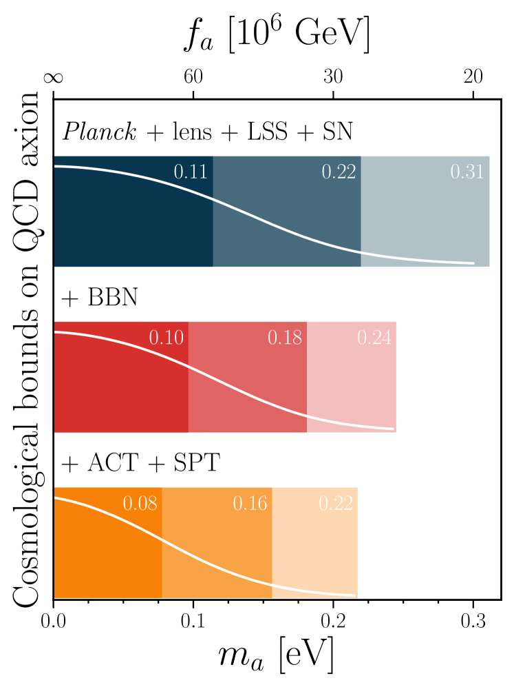
Figure 1: QCD axion mass posterior distribution from present cosmological data; 68%, 95%, 99.7% highest density probability intervals are shown from darker to lighter color shade.

According to Eq. (1), a QCD axion that decouples at high temperatures from the SM bath – say at $T_{\rm dec}\gtrsim T_{\rm EW}\sim\mathcal{O}(100)$ GeV – under quite general assumptions would leave an indelible cosmological imprint at the level of $\Delta N_{\rm eff}\sim\mathcal{O}(0.01)$ Baumann et al. (2016). This could potentially be within the reach of future surveys Abazajian et al. (2019a); Aiola et al. (2022). Most notably, an axion produced below $T_{c}$ is under the spotlight of current cosmological observations. It is then possible to rule out QCD axions with $f_{a}\lesssim\mathcal{O}(10^{7})$ GeV with a greater confidence than the one offered by astrophysical probes, often model dependent and mostly in the realm of stellar physics which is affected by large uncertainties Raffelt (2008); Miller Bertolami et al. (2014); Ayala et al. (2014); Chang et al. (2018); Bar et al. (2020); Carenza et al. (2021); Buschmann et al. (2022); Dolan et al. (2022); Lella et al. (2023).

Many cosmological analyses focusing on the QCD axion Hannestad et al. (2005); Melchiorri et al. (2007); Hannestad et al. (2007, 2008, 2010); Archidiacono et al. (2013); Giusarma et al. (2014); Di Valentino et al. (2015, 2016); Archidiacono et al. (2015); Ferreira et al. (2020); D’Eramo et al. (2022b); Di Valentino et al. (2023) primarily rely on two key ingredients: i) scattering amplitudes evaluated at leading order in a chiral expansion of the axion-pion effective Lagrangian Georgi et al. (1986); ii) a Bose-Einstein distribution for the axion in the SM bath assuming fully-established thermal equilibrium Masso et al. (2002).

Interestingly, the regime of validity of i) and ii) has been overlooked until recently. In Refs. Di Luzio et al. (2021, 2022), an explicit next-to-leading-order (NLO) computation of the axion-pion rate in chiral perturbation theory ($\chi$PT) invalidated previous results, raising questions about the robustness of the bound on the QCD axion from cosmology. Furthermore, Ref. Notari et al. (2022) developed a phenomenological analysis to constrain the QCD axion mass without relying on a thermal distribution for its phase space $\mathcal{F}_{a}(E,t)$, where $E=\sqrt{|\mathbf{k}|^{2}+m_{a}^{2}}$. In particular, in a Universe that reheats at a temperature around (or above) the QCD crossover with no initial axion abundance , the assumption $\mathcal{F}_{a}=\mathcal{F}_{a}^{\rm eq}=1/(\exp(E/T)-1)$ is indeed not justified. Departures from $\mathcal{F}_{a}^{\rm eq}$ should be investigated by solving the set of momentum-dependent Boltzmann equations with a collision term characterized by the imaginary part of the axion self-energy Graf and Steffen (2011); Salvio et al. (2014); Notari et al. (2022):

$$\frac{\partial\mathcal{F}_{a}}{\partial t} - H\,|\mathbf{k}|\frac{\partial\mathcal{F}_{a}}{\partial|\mathbf{k}|}=\,\Gamma_{a}\,(\mathcal{F}^{\rm\,eq}_{a}-\mathcal{F}_{a})\ ,$$ (2)

$$\Pi_{a}^{\rm R} = i\,\int d^{4}x\,e^{i\,xk}\,\langle\,[\,\mathcal{Q}(x),\,\mathcal{Q}(0)]\Theta(t)\,\rangle\ ,$$

where $\Gamma_{a}\equiv\textrm{Im}(\Pi_{a}^{\rm R})/(Ef_{a}^{2})$, $\mathcal{Q}\equiv\alpha_{s}/(8\pi)\,G\tilde{G}$, and $\langle\dots\rangle$ implies the trace over the thermal density matrix Laine and Vuorinen (2016).

In this Letter, we follow the approach of Ref. Notari et al. (2022). We improve upon their result by conservatively using information from the Big Bang Nucleosynthesis (BBN) era, complemented with high-resolution observations of the damping tail of the Cosmic Microwave Background (CMB) power spectra from ground-based surveys Aiola et al. (2020); Balkenhol and SPT-3G Collaboration (2023). Fig. 1 shows how these improvements yield an overall 30% tighter constraint on the QCD axion mass compared to the result obtained in Ref. Notari et al. (2022). We support our findings by quantifying the theoretical systematic uncertainties of our computation. For this reason, we compare for the first time the non-thermal distribution of hot axions as a function of its mass by solving Eq. (2) with NLO $\chi$PT unitarized rates Di Luzio and Piazza (2022), with the distribution obtained from the phenomenological approach of Notari et al. (2022). We conclude with dedicated forecasts on the QCD axion mass based on: i) recent progress on non-perturbative effects in $\Pi_{a}^{\rm R}$ at $T\gtrsim T_{c}$ from lattice QCD Bonanno et al. (2023a, b) and; ii) state-of-the-art likelihoods for the sensitivity of next-generation cosmological surveys like the Simons Observatory (SO) Ade et al. (2019), CMB-S4 Abazajian et al. (2019b, 2022), and the Dark Energy Spectroscopic Instrument (DESI) Aghamousa et al. (2016).

Hot axions from pions. While the model-building landscape related to the QCD axion is rather vast Di Luzio et al. (2020), in this work we conservatively take the model-independent interaction between $a$ and the QCD topological charge $\mathcal{Q}$ to be the main phenomenological driver. In such a minimal setup, with the extra requirement of a reheating temperature being $\gtrsim T_{c}$, the axion abundance can be efficiently built up in the thermal bath from $\pi\pi\to\pi a$ scatterings, which dominate the two-point function of Eq. (2) for $T\lesssim T_{c}$. Then, the optical theorem and the chiral Lagrangian allow one to evaluate the thermalization rate $\Gamma_{a}$, a task performed at LO in $\chi$PT already three decades ago Chang and Choi (1993). Such a LO result has been extensively adopted in the community, despite the breakdown of $\chi$PT can be estimated with the appearance of resonant structures around 500 MeV Aydemir et al. (2012). This becomes problematic when considering that the mean energy of a pion in the SM bath at a temperature where it can still be considered semi-relativistic is three times larger, namely $\langle E\rangle\simeq\rho_{\pi}/n_{\pi}=\pi^{4}T/(30\,\zeta_{3})$. This implies a center of mass energy $\sqrt{s}$ for $\pi\pi$ scattering outside the regime where $\chi$PT is reliable Schenk (1993). This reasoning recently inherited further credit from the computation of the axion production rate in Refs. Di Luzio et al. (2021, 2022), that pointed out $\Gamma^{\rm(NLO)}_{a}/\Gamma^{\rm(LO)}_{a}\sim\mathcal{O}(1)$ for the $\pi^{\pm}\pi^{0}$ channel already at $T\sim 70$ MeV. In order to overcome this limitation in the evaluation of $\Gamma_{a}$ at $T\lesssim T_{c}$, two different approaches have been recently explored:

• Ref. Di Luzio and Piazza (2022) applied the Inverse Amplitude Method (IAM) originally developed in Truong (1988) and recently reviewed in Salas-Bernárdez et al. (2021) to evaluate unitary corrections to axion-pion scattering at NLO in $\chi$PT via the phase shifts induced by pion final-state interactions Watson (1952);

• Ref. Notari et al. (2022) took advantage of the symmetries of the chiral Lagrangian to show that the amplitude for $a\pi\to\pi\pi$ can be directly related to the experimentally measured pion-pion scattering up to corrections $\mathcal{O}(m_{\pi}^{2}/s)$ at all orders in the chiral expansion.

A direct comparison of the two methods through the solution of Eq. (2) has been missing. We fill this gap in Fig. 2, where we show in the inset the axion phase-space distribution from approach (I) and (II) for three different mass values within the range allowed by current experiments.

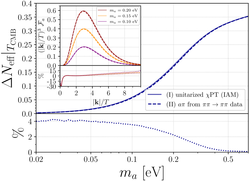
Figure 2: Extra relativistic degrees of freedom at recombination due to the hot QCD axion produced via pion scattering in the two different approaches described in the text. In the insert we compare the two methods also on the axion phase space.

In App. A we report the details to reproduce our computation of $\mathcal{F}_{a}$. The percentage difference between the two phase-space distributions for the same $m_{a}$ shows a mismatch above 10% only at the tails, suggesting a negligible impact on the cosmological data analysis. This is confirmed by examining Fig. 2, which shows $\Delta N_{\rm eff}$ as a function of the axion mass. For $m_{a}\gtrsim 0.1$ eV, the difference in terms of energy density is below 4%.

In App. B, we demonstrate that the effect of spectral distortions Ma and Bertschinger (1995); Lesgourgues and Tram (2011) in linear cosmological perturbations is minimal. This is because an analysis with the axion species described by a Bose-Einstein distribution and with the underlying $\Delta N_{\rm eff}(m_{a})$ of Fig. 2 leads to the same results. We conclude that as long as a precise evaluation of $\Delta N_{\rm eff}(m_{a})$ is considered, and axions are not treated merely as dark radiation, the cosmological bounds on $m_{a}$ in Fig. 1 remain unaffected by the choice of method (I) over (II) for the determination of $\Gamma_{a}$ .

The BBN-CMB bound. Similarly to massive neutrinos in cosmology Lesgourgues and Pastor (2006), axions manifest themselves as extra radiation in the Early Universe, altering the expansion rate and affecting the matter-radiation equality and Silk damping scales. Furthermore, they leave an important imprint on the large scale structures (LSS) when they become non-relativistic. For this reason, the QCD axion can be constrained by a set of cosmological data. These include measurements at low- and high-$\ell$ of the CMB temperature and polarization power spectra, exquisitely measured by the Planck Collaboration Aghanim et al. (2020b), as well as measurements of galaxy surveys like BOSS Alam et al. (2017), probing particularly well in the linear regime the amplitude of the matter-power spectrum at the frequencies of baryonic acoustic oscillation (BAO) peaks. In order to exploit the statistical power of the rich cosmological dataset of Refs. Aghanim et al. (2020c); Alam et al. (2017); Beutler et al. (2011); Ross et al. (2015); Alam et al. (2021); Scolnic et al. (2018); Qu et al. (2023); Carron et al. (2022), we implement the hot QCD axion as a non-cold dark-matter species in the CMB Boltzmann-solver code CLASS Lesgourgues (2011); Blas et al. (2011) using the set of phase-space distributions $\mathcal{F}_{a}$ at the core of Fig. 2. We compare theory predictions obtained in an extended $\Lambda$CDM cosmology with massive neutrinos (satisfying a lower bound of $\sum m_{\nu}>0.06~{}$eV as hinted by $\nu$-oscillation global fits Capozzi et al. (2017); de Salas et al. (2021); Gonzalez-Garcia et al. (2021)) and the QCD axion against CMB and LSS data via a Monte Carlo Markov Chain (MCMC) analysis, using the general-purpose Bayesian package Cobaya Torrado and Lewis (2021) (see App. B for more details).

In Fig. 1 we show the marginalized posterior distribution of $m_{a}$ constrained by CMB and LSS data (blue band): the 95% highest density interval (HDI) of the QCD axion mass reads $m_{a}\leq 0.22$ eV. This constraint aligns well with that from Ref. Notari et al. (2022), but is slightly stronger due to our additional inclusion of BAO measurements from luminous red galaxies observed by eBOSS Alam et al. (2021), as well as the recent combined analysis of ACT and Planck for CMB lensing Carron et al. (2022); Qu et al. (2023) . The bound does not significantly depend on the theoretical prior assumed for the mass fraction of helium-4, $Y_{P}$, despite the expected degeneracy with $N_{\rm eff}$ Schöneberg et al. (2019), which affects the free-electron fraction at recombination Lee and Ali-Haïmoud (2020) and hence Silk damping Steigman (2010). It is the inclusion of LSS data and the careful treatment of the axion as hot dark matter which breaks the degeneracy with $Y_{P}$. As we verified in App. B, allowing $Y_{P}$ to be a free parameter of the fit would only degrade the constraint by a few percent. For the combined Planck+lens+LSS+SN dataset, the $2\sigma$ upper bound on $m_{a}$ goes from 0.220 eV (when $Y_{P}$ is fixed to BBN predictions) to 0.236 eV (when $Y_{P}$ is free), a degradation of approximately 7%.

The primordial helium-4 mass fraction is not only relevant for CMB physics. It constitutes a key observable to learn about the Early Universe Sarkar (1996); Olive et al. (2000); Pospelov and Pradler (2010). It is measured at the percent level Hsyu et al. (2020) or more Kurichin et al. (2021) in metal-poor systems, while being predicted at the permil level in standard BBN as an outcome of weak interactions going out-of-equilibrium Pitrou et al. (2018). The relative number density of primordial deuterium, $D/H$, also features outstanding observational inference from fits to quasar absorption spectra Riemer-Sørensen et al. (2017); Cooke et al. (2018), and can be predicted conservatively if large systematics in the treatment of nuclear rates like $DD$ fusion Pitrou et al. (2021) are not dismissed a priori Burns et al. (2023a); Yeh et al. (2022).

In this work, we use the new publicly released package PRyMordial Burns et al. (2023b) – dedicated to the study of the physics of the Early Universe – to provide an up-to-date prediction of helium-4 and a conservative evaluation of the relative abundance of deuterium, where the key thermonuclear rates are extracted from Ref. Xu et al. (2013). We perform a set of 1300 Monte Carlo runs with PRyMordial to predict $X=\{Y_{P},D/H\}$ beyond $\Lambda$CDM as a function of $N_{\rm eff}=3.044+\Delta N_{\rm eff}$ and the cosmic baryon density $\Omega_{b}$. For each run, we extract the mean $X_{\rm th}$ and the standard deviation $\delta X_{\rm th}$ after marginalizing over thermonuclear-rate uncertainties and the neutron lifetime (whose most recent average includes only ultracold-neutron determinations Workman et al. (2022a)). Using the result in Fig. 2, we feed the updated $Y_{P}(\Omega_{b},m_{a})$ to CLASS for the computation of CMB power spectra and we implement in Cobaya a primordial element abundance Gaussian likelihood as:

$$-2\,\log\mathcal{L}_{\rm BBN}=\sum_{Y_{P},D/H}\frac{\big{(}X_{\rm exp}-X_{\rm th}(\Omega_{b},m_{a})\big{)}^{2}}{\delta X_{\rm exp}^{2}+\delta X^{2}_{\rm th}(\Omega_{b},m_{a})}\ ,$$ (3)

(see App. B for further details). Adopting the measurements on light primordial abundances recommended by the Particle Data Group Workman et al. (2022a), we obtain as a main result that BBN theory combined with observations are able to narrow the QCD axion bound at 95% HDI down to $m_{a}\leq 0.18$ eV, providing a 20% improvement from blue to red in Fig. 1.

We conclude our discussion on the current cosmological constraints on the hot QCD axion, emphasizing the importance of ground-based experiments. ACT Aiola et al. (2020) and SPT Balkenhol and SPT-3G Collaboration (2023) accurately map out the CMB temperature and polarization anisotropies at angular scales smaller than those measured by Planck. Including these datasets in our analysis, we obtain the marginalized posterior shown as the orange band in Fig. 1, ruling out axions with $m_{a}\geq 0.16$ eV at 95% HDI. Notice also that analyzing the cosmological setup without the constraint in Eq. (3) on BBN abundances would yield $m_{a}\leq 0.19$ eV at 95% probability.

In Fig. 3, we present a summary of our findings, illustrating the two-dimensional joint probability distribution of $m_{a}$ with the sum of neutrino masses.

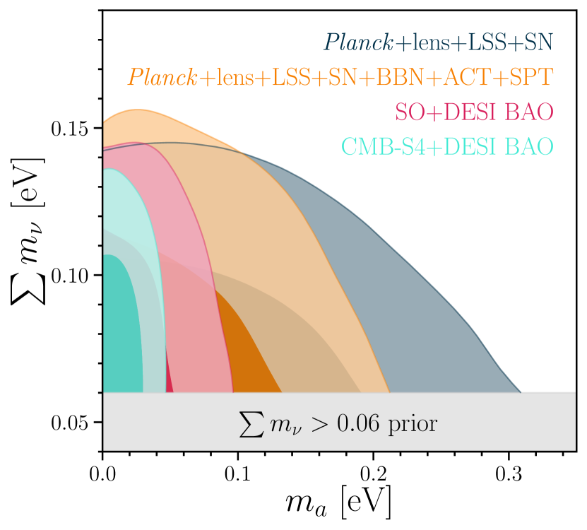
Figure 3: 68% and 95% joint HDI for the axion mass and the sum of neutrino masses from current cosmological data (blue and orange contours) and future CMB/LSS surveys (magenta and turquoise contours). See text for details on the forecast.

While the constraint on neutrinos is saturated by the statistical weight of LSS data, the bound on the QCD axion mass is improved by the addition of BBN + ACT + SPT. Figure 3 also shows that improving our knowledge on $\sum m_{\nu}$ would impact the cosmological constraint on the QCD axion .

Forecasting with sphalerons. As mentioned in the introduction, Eq. (1) provides a beacon for future searches: $\Delta N_{\rm eff}\sim\mathcal{O}(0.01)$ points to an axion decoupling temperature $T_{c}\lesssim T_{\mathrm{dec}}\lesssim\mathcal{O}(1\,\mathrm{GeV})$, i.e. in between the confined phase of QCD and the quark-gluon plasma. While the axion production rate from gluon-gluon scattering in Salvio et al. (2014) has been extended by Ref. D’Eramo et al. (2021) down to $\mathcal{O}$(GeV), Ref. Notari et al. (2022) observed that already at those temperatures, the main contribution to $\Pi_{a}^{R}$ should be of non-perturbative nature due to strong sphalerons, QCD topological configurations responsible of quark chirality-violating transitions at finite temperature McLerran et al. (1991); Giudice and Shaposhnikov (1994); Fukushima et al. (2008); Moore and Tassler (2011).

In this study, we forecast the sensitivity of future cosmological surveys to the QCD axion mass , taking advantage of the first-principle non-perturbative computation of the real-time correlator of $\mathcal{Q}$ in Eq. (2) beyond the pure Yang-Mills limit, as recently obtained by the 2+1 lattice QCD simulations above chiral crossover of Refs. Bonanno et al. (2023a, b). Adopting the best-fit results  on the sphaleron rate in Bonanno et al. (2023a), we derive the momentum-averaged one using the expected size of sphaleron configurations (see App. E of Notari et al. (2022)). In doing so, we obtain for $T_{c}\lesssim T\lesssim 600~{}$MeV a conservative estimate of the thermalization rate $\overline{\Gamma}_{a}$ governing the (integrated) Boltzmann equation of the yield $Y_{a}\equiv n_{a}/s_{\gamma}\,$:

$$\frac{dY_{a}}{dt} = \,\frac{\overline{\Gamma}_{a}}{H}\,(Y^{\rm eq}_{a}-Y_{a})\ ,$$ (4)

$$\overline{\Gamma}_{a} \simeq \kappa\,\left(\frac{T^{3}}{f_{a}^{2}}\right)\,\left(c_{0}+c_{1}\,\frac{T_{c}}{T}+c_{2}\,\frac{T_{c}^{2}}{T^{2}}\right)\,,$$

$s_{\gamma}$ being the total entropy density of the thermal bath, $\kappa=0.1$, and $c_{0,1,2}=\{0.04,-0.28,1.5\}$.

Trading time for temperature using entropy conservation, we solve Eq. (4) from 600 MeV down to $T_{c}$, and set the initial condition for the momentum-dependent Boltzmann equations in Eqs. (2) using the approximation: $\mathcal{F}_{a}(E,T_{c})\simeq\mathcal{F}^{\rm eq}_{a}(E,\overline{T})$ and determining $\overline{T}$ by $Y_{a}(T_{c})=Y^{\rm eq}_{a}(\overline{T})$. Considering an optimistic forecast, we assume that the Universe underwent reheating above the electroweak crossover, suggesting for the initial condition of Eq. (4) $Y_{a}(600\,{\rm MeV})\simeq Y^{\rm eq}_{a}(T_{\rm EW})$.

We produce our forecasts with state-of-the-art likelihoods using the dedicated routine in Cobaya for next-gen CMB/LSS experiments and adopting the expected sensitivities reported in Ade et al. (2019); Abazajian et al. (2022); Aghamousa et al. (2016) respectively for SO, CMB-S4 and DESI (BAO), as well as a fiducial $\Lambda$CDM cosmology with three degenerate neutrinos of $m_{\nu}=0.02$ eV. We forecast two different future scenarios: SO+DESI and CMB-S4+DESI. We perform an MCMC analysis for each of the cases assuming the same priors used in the real data analysis (see App. B). In the cosmological Boltzmann-solver we include the QCD axion as hot dark matter with phase-space distribution imprinted by: i) thermal equilibrium at high temperature; ii) strong-sphaleron transitions according to the averaged rate estimated for $T_{c}\lesssim T\lesssim 600~{}$MeV; iii) energy-dependent scattering with pions for $T\lesssim T_{c}$.

In Fig. 3 we show the joint $m_{a}$-$\sum m_{\nu}$ 68% and 95% HDI from our forecasts. At the 95% HDI level, SO+DESI will be sensitive to $m_{a}\lesssim 0.08$ eV, while CMB-S4+DESI could exclude axions with $m_{a}\geq 0.04~{}$eV, competitive with the current supernovae disfavoured region Lella et al. (2023). While futuristic CMB and LSS proposals like Schlegel et al. (2022); MacInnis et al. (2023) may further improve those projections, foreseeable progress in BBN physics might play a marginal role. Assuming a 50% refined inference for helium-4 and deuterium observations, and an order-of-magnitude more precise $D/H$ prediction – matching the present one for $Y_{P}$ – we added BBN to both forecasts via important sampling through Eq. (3) and improved of a few percent the bound on $m_{a}$ only for SO+DESI.

Conclusions. We determined a conservative bound on $m_{a}$ from up-to-date measurements of the CMB, including ground-based telescopes, and abundances from BBN. We treated the axion as hot dark matter evaluating its phase-space distribution beyond the thermal approximation – i.e. including spectral distortions from momentum-dependent scattering – finding $m_{a}\leq 0.16$ eV at 95% HDI, shown by the orange band in Fig. 1. We also reported the two dimensional joint posterior distributions of $m_{a}$ and $\sum m_{\nu}$ in Fig. 3 from current cosmological probes and provided a forecast for future cosmological surveys including the effect of the non-perturbative production rate expected from strong sphalerons extracted from 2+1 lattice QCD at the physical point.

While Fig. 3 captures an exciting prospect, we point out that the future for a cosmological detection of the QCD axion via primeval hot modes might be even brighter thanks to dedicated studies of the Lyman-$\alpha$ forest Iršič et al. (2023), advancements in the full-shape analysis of LSS Chudaykin et al. (2020); D’Amico et al. (2021), and progress in 21 cm intensity mapping Karkare et al. (2022).

Acknowledgements. We thank Luca Di Luzio, Peter Graham, Maxim Pospelov, Neelima Sehgal, Luca Silvestrini and Wei Xue for discussions. G.G.d.C. is grateful to SCGP, F.B. to INFN Rome and Sapienza, M.V. to SITP and SLAC, for the hospitality during the completion of the work. F.B. would like to thank Emmanuel Schaan and Kimmy Wu for stylistic suggestions on Fig. 1. F.B. acknowledges support by the Department of Energy, Contract DE-AC02-76SF00515.

Appendix A Axion thermalization rate

In this appendix we report more details about the numerical computation of the thermalization rate for hot axion production and the evaluation of the axion phase-space distribution. The momentum-dependent thermalization rate $\Gamma_{a}$ defined in Eq. (2) can be explicitly written for the process $\pi\pi\to\pi a$ as follows:

$$\mathcal{F}_{a}^{\rm eq}\,\Gamma_{a}=\frac{1}{2\,E}\int\biggl{(}\prod_{i=1}^{3}\frac{d^{3}\mathbf{k}_{i}}{(2\pi)^{3}\,2\,E_{i}}\biggr{)}\mathcal{F}_{1}^{\mathrm{eq}}\mathcal{F}_{2}^{\mathrm{eq}}(1+\mathcal{F}_{3}^{\mathrm{eq}})(2\pi)^{4}\delta^{(4)}(k_{1}^{\mu}+k_{2}^{\mu}-k_{3}^{\mu}-k^{\mu})\,|\mathcal{M}|^{2},$$ (5)

where $|\mathcal{M}|^{2}$ is the modulus squared of the scattering amplitude (summed over initial and final spins) and $k_{i}^{\mu}$ with $i=1,\,2,\,3$ are the 4-momenta of the incoming pions and the outgoing one, respectively, while $k$ is the 4-momentum of the axion. Following similar steps carried out in the literature for the collision term of the momentum-dependent Boltzmann equations of neutrinos Yueh and Buchler (1976); Hannestad and Madsen (1995), we can rewrite the above as:

$$\Gamma_{a}=\frac{\exp(E/T)-1}{16\pi^{4}\,E}\int_{0}^{\infty}\biggl{(}\prod_{i=1}^{2}\frac{d|\mathbf{k}_{i}||\mathbf{k_{i}}|^{2}}{E_{i}}\biggr{)}\int_{-1}^{1}dc_{\alpha}\int_{-1}^{1}dc_{\beta}\,\mathcal{F}_{1}^{\mathrm{eq}}\mathcal{F}_{2}^{\mathrm{eq}}(1+\mathcal{F}_{3}^{\mathrm{eq}})\frac{\Theta(E_{1}+E_{2}-E)\Theta(1-c_{\gamma_{0}}^{2})}{|h^{\prime}(\gamma_{0})|}|\mathcal{M}|^{2},$$ (6)

where $h(\gamma)=k_{3}^{2}-m_{3}^{2}$ and $\gamma_{0}$ are the zeros of $h(\gamma)$. The scattering angles $\alpha$, $\beta$ and $\gamma$ are defined as:

$$c_{\alpha}=\cos\alpha=\frac{\mathbf{k}_{1}\cdot\mathbf{k}_{2}}{|\mathbf{k}_{1}||\mathbf{k}_{2}|},\qquad c_{\beta}=\cos\beta=\frac{\mathbf{k}_{1}\cdot\mathbf{k}}{|\mathbf{k}_{1}||\mathbf{k}|},\qquad\frac{\mathbf{k}_{2}\cdot\mathbf{k}}{|\mathbf{k}_{2}||\mathbf{k}|}=\cos\alpha\cos\beta+\sin\alpha\sin\beta\cos\gamma\ ,$$ (7)

and $\mathcal{F}_{3}^{\mathrm{eq}}$ is now a function of $|\mathbf{{k}_{1}}|$ and $|\mathbf{k}_{2}|$ via energy conservation. Also the amplitude $|\mathcal{M}|^{2}$, which depends on the Mandelstam variables $s,t,u$ of the $2\to 2$ process, can be expressed as a function of the 3-momenta $|\mathbf{{k}_{1}}|$ and $|\mathbf{{k}_{2}}|$.

For the numerical analysis, we used $f_{\pi}=92.3$ MeV, an average pion mass $m_{\pi}=138$ MeV and the isospin-suppression factor: $(m_{d}-m_{u})/(m_{d}+m_{u})\simeq 0.47$ Workman et al. (2022b), where $m_{u}$ and $m_{d}$ are the up- and down-quark masses. The multi-dimensional integration was performed with use of the Python library vegas Lepage (2021). The missing ingredient of equation (7) – the modulus square of the amplitude – is described in the following for the two different methods outlined in the text, see also Notari et al. (2022); Di Luzio et al. (2022) for more details.

A.1 Inverse Amplitude Method

The amplitude $\mathcal{M}$ can be conveniently decomposed in a basis with definite total isospin $I$; in doing so, one can obtain the following relations involving Clebsch-Gordan weights Di Luzio et al. (2022):

$$\mathcal{M}_{+0} = -\frac{A_{1}+A_{2}^{\prime}}{\sqrt{2}}=-\mathcal{M}_{-0},\qquad\mathcal{M}_{\pm\mp}=-\frac{\sqrt{2}A_{0}+A_{2}}{\sqrt{6}},$$ (8)

$$\mathcal{M}_{0+} = \frac{A_{1}-A_{2}^{\prime}}{\sqrt{2}}=-\mathcal{M}_{0-},\qquad\quad\mathcal{M}_{00}=-\frac{A_{0}-\sqrt{2}A_{2}}{\sqrt{3}}.$$

Notice that the amplitudes in the defined total isospin basis $A_{2}$ and $A_{2}^{\prime}$ are different because the axion coupling to pions violates isospin, and $\mathcal{M}_{+-}=\mathcal{M}_{-+}$ because of charge-conjugation symmetry.

We can now further project the amplitudes with defined total isospin into a basis of states with well-defined total angular momentum $J$, obtaining

$$A_{I}(s,\cos\theta)=\sum_{J=0}^{\infty}(2J+1)P_{J}(\cos\theta)A_{IJ}(s),$$ (9)

where $\cos\theta$ is the scattering angle in the center of mass frame, and $P_{J}(\cos\theta)$ are Legendre polynomials. We can then apply the inverse amplitude method Salas-Bernárdez et al. (2021) at the next-to-leading-order expressing perturbatively $A_{IJ}$ as:

$$A_{IJ}(s)=\frac{A_{IJ}^{(2)}(s)}{1-A_{IJ}^{(4)}(s)/A_{IJ}^{(2)}(s)},$$ (10)

where by $A_{IJ}^{(2n)}$ we denote the amplitudes calculated in $\chi$PT up to $\mathcal{O}(p^{2n})$ from the partial-wave decomposition:

$$A_{IJ}^{(2n)}(s)=\frac{1}{2}\int_{-1}^{+1}d\cos\theta\,P_{J}(\cos\theta)A_{I}^{(2n)}(s,\cos\theta).$$ (11)

In our computation we include the contributions coming from S-wave ($J=0$, $I=0,\,2$) and P-wave ($J=1$, $I=1$), and adopt the analytical expression of the amplitudes for the $\pi\pi\to\pi a$ reported in Di Luzio et al. (2022). For our analysis we used the following low-energy constants: $\bar{\ell}_{1}=-0.525$ Dobado and Pelaez (1997), $\bar{\ell}_{2}=5.425$ Dobado and Pelaez (1997), $\bar{\ell}_{3}=3.53$ Aoki et al. (2022), $\bar{\ell}_{4}=4.73$ Aoki et al. (2022) and $\ell_{7}=0.007$ Grilli di Cortona et al. (2016).

A.2 Phenomenological Approach

The amplitude from the phenomenological partial-wave phases of $\pi\pi$ scattering is obtained by decomposing $\mathcal{M}$ in the charged basis into a basis with well-defined isospin, and then expanding each amplitude into partial waves. Following the notation of Gasser and Leutwyler (1984), the partial-wave amplitudes are related to the real phase shifts $\delta_{J}^{I}$ as:

$$t_{J}^{I}(s)=\sqrt{\frac{s}{s-4m_{\pi}^{2}}}\left(\frac{1}{\cot\delta_{J}^{I}(s)-i}\right)\ ,$$ (12)

where the $\delta_{J}^{I}(s)$ are parameterised as in Garcia-Martin et al. (2011). We include only the S- and P-wave phase shift, since other terms give a negligible contribution to the rates. We find the modulus squared of the total amplitude $\pi\pi\to\pi a$ to be given by:

$$|\mathcal{M}|^{2}=\frac{128\pi^{2}}{3}\left(\frac{m_{d}-m_{u}}{m_{d}+m_{u}}\right)^{2}\left(\frac{f_{\pi}}{f_{a}}\right)^{2}\left(|t_{0}^{0}|^{2}+27\,|\cos\theta\,t_{1}^{1}|^{2}+5\,|t_{0}^{2}|^{2}\right).$$ (13)

A.3 The Strong Sphaleron Rate

The axion thermalization rate at zero-momentum from strong-sphaleron transitions is taken from the results of the lattice QCD simulation at the physical point for 2+1 flavors of Ref.s Bonanno et al. (2023a, b), according to the Monte Carlo simulations performed in that work for five sampling temperatures: $T=$230, 300, 365, 430 and 570 MeV. We adopted the phenomenological parameterization given by the power-law fit:

$$\Gamma_{\rm sph}^{(0)}\equiv\Gamma_{\rm sph}(|\mathbf{k}|=0)=\Lambda_{0}^{4}\ (T/T_{c})^{\epsilon}\ ,$$ (14)

where $\Lambda_{0}\simeq 142.3~{}$MeV, $\epsilon\simeq 1.81$ , $T_{c}=155~{}$MeV.

We notice that the above parameterization (adopted in the range $150~{}{\rm MeV}\lesssim T\lesssim 600~{}$MeV) gives a slightly smaller $\Delta N_{\rm eff}(m_{a})$ in the final computation with respect to the one obtained from the semiclassically-inspired fit reported in the same Ref.s Bonanno et al. (2023a, b). To compute the axion phase-space distribution with the inclusion of non-perturbative effects, we conservatively estimated the momentum-averaged axion rate $\overline{\Gamma}_{a}$ using the fact that $\Gamma_{\rm sph}$ should be the same within a shell of momentum $|\mathbf{k}|<|\mathbf{k_{s}}|$, with $|\mathbf{k_{s}}|$ set by the expected sphaleron size, $\mathcal{O}(\alpha_{s}T)$; hence, we obtained:

$$n_{a}^{\rm eq}\,\overline{\Gamma}_{a}\simeq\frac{1}{8\pi^{2}f_{a}^{2}}\int_{0}^{1/(3\alpha_{s}T)}d|\mathbf{k}||\mathbf{k}|\frac{\mathcal{F}^{\rm eq}_{a}}{(1+\mathcal{F}^{\rm eq}_{a})}\,\Gamma_{\rm sph}^{(0)}\ ,$$ (15)

see also Appendix E of Ref. Notari et al. (2022) for more details. As described in the main text, the solution of the (integrated) Boltzmann equation governed by $\overline{\Gamma}_{a}$ allows one to estimate the temperature which sets the initial condition $\mathcal{F}_{a}>0$ at $T_{c}$ adopted for our forecasts.

Appendix B Cosmological Analysis

In this appendix, we detail the integration of hot axions into the Boltzmann-solver CLASS (Lesgourgues and Tram, 2011) and provide further details on our Markov Chain Monte Carlo (MCMC) analyses using Cobaya (Torrado and Lewis, 2021).

B.1 Axions As Hot Dark Matter

Our cosmological analysis treats the axion as an additional non-cold dark matter (ncdm) species. This is accomplished by coding a new phase-space distribution in the background.c source file. In our numerical analysis, for a grid of masses $m_{a}$ we have approximated the numerical phase-space distribution obtained from the solution to the momentum-Boltzmann equations with a Fermi-Dirac o Bose-Einstein distribution with non-zero chemical potential. We have verified the accuracy of this approximation over a range of scales $0.04\lesssim|\mathbf{k}|/T\lesssim 150$ and masses $0.01\lesssim m_{a}/\mathrm{eV}\lesssim 4$ and found very good agreement. Although the phase-space distribution above solely depends on $|\mathbf{k}|/T$ and $m_{a}$, CLASS requires us to assign a temperature $T_{\rm ncdm}$ to the non-cold dark matter species. This temperature essentially serves as an overall normalization of the phase-space distribution. We properly set this temperature to be: $T_{a}=(4/11)^{1/3}\left[g_{*s}(3\,\text{MeV})/g_{*s}(30\,\text{MeV})\right]^{1/3}$, where $g_{*s}$ is the number of entropic degrees of freedom of the thermal bath, similarly to what already highlighted in Ref. Notari et al. (2022).

When neglecting spectral distortions and modeling the QCD axion with a Bose-Einstein distribution, we set the species temperature to:

$$T_{a}(m_{a})=\left(\frac{4}{11}\right)^{1/3}\left[\frac{7}{4}\Delta N_{\rm eff}(m_{a})\right]^{1/4}\,\text{eV},$$ (16)

where $\Delta N_{\rm eff}(m_{a})$ is an analytical fit to the numerically evaluated contribution of the QCD axion to the effective number of relativistic degrees of freedom.

B.2 Cosmological Inference Framework

Our baseline cosmology extends the $\Lambda$CDM model to include neutrinos and the QCD axion, which are treated as hot dark matter species, and is built on purely adiabatic scalar fluctuations.

This baseline model comprises a total of eight cosmological parameters, including the physical density of cold dark matter ($\Omega_{\rm c}h^{2}$), the physical density of baryons ($\Omega_{\rm b}h^{2}$), the approximated angular size of the sound horizon at recombination ($100\,\theta_{\rm s}$), the optical depth at reionization ($\tau$), the amplitude of curvature perturbations at $\hat{k}=0.05$ Mpc^-1 ($A_{s}$), and the spectral index ($n_{s}$) of the power law power spectrum of primordial scalar fluctuations.

In addition to these six standard $\Lambda$CDM parameters, we include the axion mass $m_{a}$ and the sum of the active neutrino masses $\sum m_{\nu}$. We assume these to be a degenerate combination of three equally massive neutrinos, as done in the publications of the Planck Collaboration (Lesgourgues and Pastor, 2006; Aghanim et al., 2019). The lensed CMB and CMB lensing potential power spectra are computed using the CLASS Boltzmann code (v3.3.1). To infer cosmological parameter constraints, we sample the posterior space using the Metropolis-Hastings sampler with adaptive covariance learning, provided in the Markov Chain Monte Carlo (MCMC) Cobaya package Torrado and Lewis (2021). When sampling the parameter space, we adopt the priors listed in Tab. 1. Note, in particular, that we assume $m_{\nu}\geq 0.02$ eV for three degenerate neutrinos to enforce the lower bound on the sum of the neutrino masses $\sum m_{\nu}\geq 0.06$ eV from oscillation measurements Capozzi et al. (2017); de Salas et al. (2021); Gonzalez-Garcia et al. (2021). For each cosmological model and dataset combination, we run four MPI parallel chains (each one using four OpenMP processes) until the Gelman–Rubin statistic reaches a convergence threshold of $R-1\leq 0.02$.

Table 1: Cosmological parameters varied in this work and their respective priors. $\mathcal{U}(a,b)$ denotes a uniform distribution between $[a,b]$, while $\mathcal{N}(\mu,\sigma)$ indicates a Gaussian distribution with mean $\mu$ and variance $\sigma^{2}$. Note that when analyzing mock data from future CMB surveys, we adopt a Planck-based Gaussian prior on $\tau\sim\mathcal{N}(0.055,0.007)$.

Parameter	${\Omega_{b}h^{2}}$	$\Omega_{\rm c}h^{2}$	$100\,\theta_{s}$	$\tau$	$n_{s}$	$\ln(10^{10}A_{\rm s})$	$\sum m_{\rm\nu}$ [eV]	$m_{a}$ [eV]	$Y_{P}$
Prior	$\,\mathcal{U}(0.005,0.1)\,$	$\,\mathcal{U}(0.001,0.99)\,$	$\,\mathcal{U}(0.5,10)\,$	$\,\mathcal{U}(0.01,0.8)\,$	$\,\mathcal{U}(0.8,1.2)\,$	$\,\mathcal{U}(1.6,3.9)\,$	$\,\mathcal{U}(0.06,5)\,$	$\,\mathcal{U}(0,4)\,$	$\,\mathcal{U}(0.1,0.5)\,$

B.3 Cosmological Datasets

Our cosmological analysis incorporates seven distinct types of observations: primary CMB, CMB lensing, BAO, redshift space distortions (RSD), Type Ia supernova (SNeIa) distance moduli, and the observational inference of the primordial abundances of the mass fraction of helium-4, $Y_{P}$, and of the relative number density of deuterium, $D/H$.

For primary CMB, we utilize the CMB temperature and polarization anisotropies measurements as presented in the Planck 2018 data release Aghanim et al. (2020c). Specifically, we combine both the low- and high-$\ell$ temperature and polarization likelihoods derived from PR3 maps. This dataset is referred to as ‘Planck’ in our figures. We supplement Planck observations with high-resolution CMB temperature and polarization measurements at intermediate and small angular scales from ground-based experiments. Specifically, we incorporate the Atacama Cosmology Telescope (ACT) DR4 $TT/TE/EE$ results from Aiola et al. (2020) and the 2018 South Pole Telescope (SPT) SPT-3G $TT/TE/EE$ measurements from Balkenhol and SPT-3G Collaboration (2023). We denote the combination of these two datasets as ‘ACT+SPT’.

We utilize measurements of the CMB lensing power spectrum derived from a joint analysis of Planck PR4 Carron et al. (2022) and ACT DR6 data Qu et al. (2023). This data product is referred to as ‘lens’.

For BAO, we use likelihoods obtained from spectroscopic galaxy surveys, including the BOSS (Baryon Oscillation Spectroscopic Survey) DR12 Alam et al. (2017), SDSS MGS (Sloan Digital Sky Survey Main Galaxy Sample; Ross et al., 2015), 6dFGS (Six-degree Field Galaxy Survey; Beutler et al., 2011), and eBOSS DR16 Luminous Red Galaxy (LRG Alam et al., 2021) surveys. Additionally, we use measurements of the growth rate of structure $f\sigma_{8}$ from BOSS Alam et al. (2017). Together with BAO, we label this dataset combination as ‘LSS’.

The SNeIa distance moduli measurements are from the Pantheon sample Scolnic et al. (2018). We refer to this dataset as ‘SN’.

Finally, we use the measurements on light primordial abundances recommended by the Particle Data Group Workman et al. (2022a), namely: $Y_{P}=0.245\pm 0.003$ and $D/H\times 10^{5}=2.547\pm 0.025$. We refer to this dataset as ‘BBN’.

We also forecast the cosmological sensitivity of next-generation CMB and LSS surveys to the QCD axion mass. We consider the $TT/TE/EE/\phi\phi$ data vector from two representative upcoming ground-based CMB surveys, Simons Observatory (SO) Ade et al. (2019) and CMB-S4 (Abazajian et al., 2019b, 2022). The effective temperature and polarization noise curves are calculated after multi-frequency component-separation while CMB lensing is assumed to be reconstructed with a minimum-variance quadratic estimator . We assume a sky fraction of $f_{\rm sky}=0.4$ for both surveys and use CMB information between $30\leq\ell\leq 3000$ in temperature and between $30\leq\ell\leq 5000$ for polarization and lensing. The CMB power spectra likelihood is the one from Hamimeche and Lewis (2008) (specifically we use the CMBlikes likelihood class in Cobaya). Note that when producing forecasts using mock SO and CMB-S4 data, we add a Planck-based Gaussian prior on the optical depth $\tau\sim\mathcal{N}(0.055,0.007)$ to account for the missing large-scale ($\ell\lesssim 30$) polarization information from the ground.

We also include future BAO data in the form of $r_{s}/D_{V}$ measurements from DESI Aghamousa et al. (2016), where $D_{V}$ is the volume averaged distance and $r_{s}$ is the sound horizon at the drag epoch when photons and baryons decouple. Specifically, we consider the baseline DESI survey, covering 14000 deg² and targeting bright galaxies, luminous red galaxies, and emission-line galaxies in the redshift range $z\in[0.15,1.85]$ with 18 bins equally spaced redshift bin.

The fiducial cosmology used to generate the mock CMB/BAO data vectors assumes three equally massive neutrinos with total mass $\sum m_{\nu}=0.06$ eV and a vanishing axion mass, $m_{a}=0$ eV.

B.4 BBN Likelihood

The BBN likelihood reported in Eq. (3) is modeled as a Gaussian and is based on a set of 1300 Monte Carlo (MC) runs with the code PRyMordial to predict light abundances as a function of $N_{\rm eff}$ and $\Omega_{b}$. Each of the MC runs comprised $10^{4}$ events at fixed baryon density and relativistic number of degrees of freedom. We varied 12 nuisance parameters related to the key nuclear rates for helium and deuterium production, adopting log-normal distributions as detailed in Ref. Coc et al. (2014) and explicitly shown in one of the examples given in Ref. Burns et al. (2023b); we also assigned a Gaussian prior on the neutron lifetime according to what has been recently recommended by the Particle Data Group Workman et al. (2022a): $\tau_{n}=(878.4\pm 0.5$) s.

For each MC run we have computed mean and standard deviation from the posterior distribution of $Y_{P}$ and $D/H$. The corresponding numerical table has been publicly released for the general usage of the community and can be found at the repository of the code, https://github.com/vallima/PRyMordial.

B.5 Cosmological Tests

We mention here some robustness tests performed at the cosmological inference level. In particular, we have tested how including spectral distortions in our analysis only at the level of the background, but not at linear cosmological perturbations one, yields a very similar bound on the QCD axion. In the left panel of Fig. 4 we support this statement analyzing the baseline cosmological dataset Planck+lens+LSS+SN in the two cases, obtaining the following bounds on the axion mass: $m_{a}<0.220$ eV (full) vs $m_{a}<0.214$ eV (BE), i.e. a $\sim 3\%$ relative difference.

In addition, in the right panel of Fig. 4 we zoom on the role of the theoretical prior of helium-4 for the bound of the QCD axion. We note according to the triangle plot produced and cosmological setups shown that without the inclusion of LSS in the analysis (especially in the form of BAO data) it is not possible to constrain precisely any hot dark matter species unless the theoretical knowledge of helium-4 from BBN theory is exploited in the analysis.

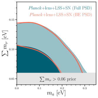
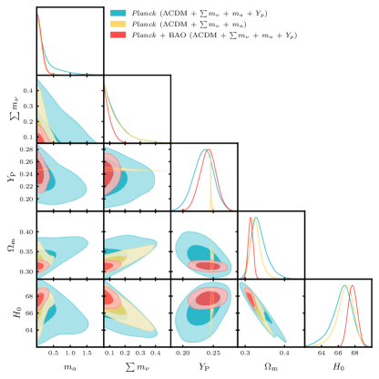
Figure 4: In the left pane we show the comparison between the 1 and $2\sigma$ contours inferred from the analysis of Planck + lens + LSS + SN data under the assumption of a Bose-Einstein thermal distribution for the axion (empty red contours) or using the full numerical phase-space distribution (filled blue contours). In the right panel we show an interesting subset of the triangle plot of different cosmological setups to highlight the importance of BAO in respect to the theoretical knowledge of the helium-4 in order to constrain hot dark matter species.

References

- Peccei and Quinn (1977a) R. D. Peccei and H. R. Quinn, Phys. Rev. Lett. 38, 1440 (1977a).
- Peccei and Quinn (1977b) R. D. Peccei and H. R. Quinn, Phys. Rev. D 16, 1791 (1977b).
- Weinberg (1978) S. Weinberg, Phys. Rev. Lett. 40, 223 (1978).
- Wilczek (1978) F. Wilczek, Phys. Rev. Lett. 40, 279 (1978).
- Baker et al. (2006) C. A. Baker et al., Phys. Rev. Lett. 97, 131801 (2006), arXiv:hep-ex/0602020 .
- Pendlebury et al. (2015) J. M. Pendlebury et al., Phys. Rev. D 92, 092003 (2015), arXiv:1509.04411 [hep-ex] .
- Abel et al. (2020) C. Abel et al., Phys. Rev. Lett. 124, 081803 (2020), arXiv:2001.11966 [hep-ex] .
- Vafa and Witten (1984) C. Vafa and E. Witten, Phys. Rev. Lett. 53, 535 (1984).
- Dvali (2022) G. Dvali, (2022), arXiv:2209.14219 [hep-ph] .
- Preskill et al. (1983) J. Preskill, M. B. Wise, and F. Wilczek, Phys. Lett. 120B, 127 (1983).
- Abbott and Sikivie (1983) L. F. Abbott and P. Sikivie, Phys. Lett. 120B, 133 (1983).
- Dine and Fischler (1983) M. Dine and W. Fischler, Phys. Lett. 120B, 137 (1983).
- Davis (1986) R. L. Davis, Phys. Lett. B 180, 225 (1986).
- Turner (1987) M. S. Turner, Phys. Rev. Lett. 59, 2489 (1987), [Erratum: Phys.Rev.Lett. 60, 1101 (1988)].
- Kolb and Turner (1990) E. W. Kolb and M. S. Turner, The Early Universe, Vol. 69 (1990).
- Berezhiani et al. (1992) Z. Berezhiani, A. Sakharov, and M. Khlopov, Sov. J. Nucl. Phys. 55, 1063 (1992).
- Chang and Choi (1993) S. Chang and K. Choi, Phys. Lett. B 316, 51 (1993), arXiv:hep-ph/9306216 .
- Baumann et al. (2016) D. Baumann, D. Green, and B. Wallisch, Phys. Rev. Lett. 117, 171301 (2016), arXiv:1604.08614 [astro-ph.CO] .
- D’Eramo et al. (2022a) F. D’Eramo, E. Di Valentino, W. Giarè, F. Hajkarim, A. Melchiorri, O. Mena, F. Renzi, and S. Yun, JCAP 09, 022 (2022a), arXiv:2205.07849 [astro-ph.CO] .
- Aoki et al. (2006) Y. Aoki, Z. Fodor, S. D. Katz, and K. K. Szabo, Phys. Lett. B 643, 46 (2006), arXiv:hep-lat/0609068 .
- Borsanyi et al. (2010) S. Borsanyi, Z. Fodor, C. Hoelbling, S. D. Katz, S. Krieg, C. Ratti, and K. K. Szabo (Wuppertal-Budapest), JHEP 09, 073 (2010), arXiv:1005.3508 [hep-lat] .
- Bazavov et al. (2012) A. Bazavov et al., Phys. Rev. D 85, 054503 (2012), arXiv:1111.1710 [hep-lat] .
- Grilli di Cortona et al. (2016) G. Grilli di Cortona, E. Hardy, J. Pardo Vega, and G. Villadoro, JHEP 01, 034 (2016), arXiv:1511.02867 [hep-ph] .
- Gorghetto and Villadoro (2019) M. Gorghetto and G. Villadoro, JHEP 03, 033 (2019), arXiv:1812.01008 [hep-ph] .
- Aghanim et al. (2020a) N. Aghanim et al. (Planck), Astron. Astrophys. 641, A6 (2020a), arXiv:1807.06209 [astro-ph.CO] .
- Note (1) The constraint corresponds to the 95% probability bound from the Planck Collaboration with no prior on helium-4.
- D’Eramo et al. (2021) F. D’Eramo, F. Hajkarim, and S. Yun, JHEP 10, 224 (2021), arXiv:2108.05371 [hep-ph] .
- Abazajian et al. (2019a) K. Abazajian et al., (2019a), arXiv:1907.04473 [astro-ph.IM] .
- Aiola et al. (2022) S. Aiola et al. (CMB-HD), (2022), arXiv:2203.05728 [astro-ph.CO] .
- Raffelt (2008) G. G. Raffelt, Lect. Notes Phys. 741, 51 (2008), arXiv:hep-ph/0611350 .
- Miller Bertolami et al. (2014) M. M. Miller Bertolami, B. E. Melendez, L. G. Althaus, and J. Isern, JCAP 10, 069 (2014), arXiv:1406.7712 [hep-ph] .
- Ayala et al. (2014) A. Ayala, I. Dominguez, M. Giannotti, A. Mirizzi, and O. Straniero, Phys. Rev. Lett. 113, 191302 (2014), arXiv:1406.6053 [astro-ph.SR] .
- Chang et al. (2018) J. H. Chang, R. Essig, and S. D. McDermott, JHEP 09, 051 (2018), arXiv:1803.00993 [hep-ph] .
- Bar et al. (2020) N. Bar, K. Blum, and G. D’Amico, Phys. Rev. D 101, 123025 (2020), arXiv:1907.05020 [hep-ph] .
- Carenza et al. (2021) P. Carenza, B. Fore, M. Giannotti, A. Mirizzi, and S. Reddy, Phys. Rev. Lett. 126, 071102 (2021), arXiv:2010.02943 [hep-ph] .
- Buschmann et al. (2022) M. Buschmann, C. Dessert, J. W. Foster, A. J. Long, and B. R. Safdi, Phys. Rev. Lett. 128, 091102 (2022), arXiv:2111.09892 [hep-ph] .
- Dolan et al. (2022) M. J. Dolan, F. J. Hiskens, and R. R. Volkas, JCAP 10, 096 (2022), arXiv:2207.03102 [hep-ph] .
- Lella et al. (2023) A. Lella, P. Carenza, G. Co’, G. Lucente, M. Giannotti, A. Mirizzi, and T. Rauscher, (2023), arXiv:2306.01048 [hep-ph] .
- Hannestad et al. (2005) S. Hannestad, A. Mirizzi, and G. Raffelt, JCAP 07, 002 (2005), arXiv:hep-ph/0504059 .
- Melchiorri et al. (2007) A. Melchiorri, O. Mena, and A. Slosar, Phys. Rev. D 76, 041303 (2007), arXiv:0705.2695 [astro-ph] .
- Hannestad et al. (2007) S. Hannestad, A. Mirizzi, G. G. Raffelt, and Y. Y. Y. Wong, JCAP 08, 015 (2007), arXiv:0706.4198 [astro-ph] .
- Hannestad et al. (2008) S. Hannestad, A. Mirizzi, G. G. Raffelt, and Y. Y. Y. Wong, JCAP 04, 019 (2008), arXiv:0803.1585 [astro-ph] .
- Hannestad et al. (2010) S. Hannestad, A. Mirizzi, G. G. Raffelt, and Y. Y. Y. Wong, JCAP 08, 001 (2010), arXiv:1004.0695 [astro-ph.CO] .
- Archidiacono et al. (2013) M. Archidiacono, S. Hannestad, A. Mirizzi, G. Raffelt, and Y. Y. Y. Wong, JCAP 10, 020 (2013), arXiv:1307.0615 [astro-ph.CO] .
- Giusarma et al. (2014) E. Giusarma, E. Di Valentino, M. Lattanzi, A. Melchiorri, and O. Mena, Phys. Rev. D 90, 043507 (2014), arXiv:1403.4852 [astro-ph.CO] .
- Di Valentino et al. (2015) E. Di Valentino, S. Gariazzo, E. Giusarma, and O. Mena, Phys. Rev. D 91, 123505 (2015), arXiv:1503.00911 [astro-ph.CO] .
- Di Valentino et al. (2016) E. Di Valentino, E. Giusarma, M. Lattanzi, O. Mena, A. Melchiorri, and J. Silk, Phys. Lett. B 752, 182 (2016), arXiv:1507.08665 [astro-ph.CO] .
- Archidiacono et al. (2015) M. Archidiacono, T. Basse, J. Hamann, S. Hannestad, G. Raffelt, and Y. Y. Y. Wong, JCAP 05, 050 (2015), arXiv:1502.03325 [astro-ph.CO] .
- Ferreira et al. (2020) R. Z. Ferreira, A. Notari, and F. Rompineve, (2020), arXiv:2012.06566 [hep-ph] .
- D’Eramo et al. (2022b) F. D’Eramo, F. Hajkarim, and S. Yun, Phys. Rev. Lett. 128, 152001 (2022b), arXiv:2108.04259 [hep-ph] .
- Di Valentino et al. (2023) E. Di Valentino, S. Gariazzo, W. Giarè, A. Melchiorri, O. Mena, and F. Renzi, Phys. Rev. D 107, 103528 (2023), arXiv:2212.11926 [astro-ph.CO] .
- Georgi et al. (1986) H. Georgi, D. B. Kaplan, and L. Randall, Phys. Lett. B 169, 73 (1986).
- Masso et al. (2002) E. Masso, F. Rota, and G. Zsembinszki, Phys. Rev. D 66, 023004 (2002), arXiv:hep-ph/0203221 .
- Di Luzio et al. (2021) L. Di Luzio, G. Martinelli, and G. Piazza, Phys. Rev. Lett. 126, 241801 (2021), arXiv:2101.10330 [hep-ph] .
- Di Luzio et al. (2022) L. Di Luzio, J. Martin Camalich, G. Martinelli, J. A. Oller, and G. Piazza, (2022), arXiv:2211.05073 [hep-ph] .
- Notari et al. (2022) A. Notari, F. Rompineve, and G. Villadoro, (2022), arXiv:2211.03799 [hep-ph] .
- Note (2) This is the proper initial condition to claim a conservative bound on in light of an experimental sensitivity to .
- Graf and Steffen (2011) P. Graf and F. D. Steffen, Phys. Rev. D 83, 075011 (2011), arXiv:1008.4528 [hep-ph] .
- Salvio et al. (2014) A. Salvio, A. Strumia, and W. Xue, JCAP 01, 011 (2014), arXiv:1310.6982 [hep-ph] .
- Laine and Vuorinen (2016) M. Laine and A. Vuorinen, Basics of Thermal Field Theory, Vol. 925 (Springer, 2016) arXiv:1701.01554 [hep-ph] .
- Aiola et al. (2020) S. Aiola et al. (ACT), JCAP 12, 047 (2020), arXiv:2007.07288 [astro-ph.CO] .
- Balkenhol and SPT-3G Collaboration (2023) L. Balkenhol and SPT-3G Collaboration, Phys. Rev. D 108, 023510 (2023), arXiv:2212.05642 [astro-ph.CO] .
- Di Luzio and Piazza (2022) L. Di Luzio and G. Piazza, (2022), arXiv:2206.04061 [hep-ph] .
- Bonanno et al. (2023a) C. Bonanno, F. D’Angelo, M. D’Elia, L. Maio, and M. Naviglio, (2023a), arXiv:2308.01287 [hep-lat] .
- Bonanno et al. (2023b) C. Bonanno, F. D’Angelo, M. D’Elia, L. Maio, and M. Naviglio, in 26th High-Energy Physics International Conference in QCD (2023) arXiv:2309.13327 [hep-lat] .
- Ade et al. (2019) P. Ade et al. (Simons Observatory), JCAP 02, 056 (2019), arXiv:1808.07445 [astro-ph.CO] .
- Abazajian et al. (2019b) K. N. Abazajian et al., “Cmb-s4 decadal survey apc white paper,” (2019b), arXiv:1908.01062 [astro-ph.IM] .
- Abazajian et al. (2022) K. Abazajian et al. (CMB-S4), (2022), arXiv:2203.08024 [astro-ph.CO] .
- Aghamousa et al. (2016) A. Aghamousa et al. (DESI), (2016), arXiv:1611.00036 [astro-ph.IM] .
- Di Luzio et al. (2020) L. Di Luzio, M. Giannotti, E. Nardi, and L. Visinelli, Phys. Rept. 870, 1 (2020), arXiv:2003.01100 [hep-ph] .
- Aydemir et al. (2012) U. Aydemir, M. M. Anber, and J. F. Donoghue, Phys. Rev. D 86, 014025 (2012), arXiv:1203.5153 [hep-ph] .
- Schenk (1993) A. Schenk, Phys. Rev. D 47, 5138 (1993).
- Truong (1988) T. N. Truong, Phys. Rev. Lett. 61, 2526 (1988).
- Salas-Bernárdez et al. (2021) A. Salas-Bernárdez, F. J. Llanes-Estrada, J. Escudero-Pedrosa, and J. A. Oller, SciPost Phys. 11, 020 (2021), arXiv:2010.13709 [hep-ph] .
- Watson (1952) K. M. Watson, Phys. Rev. 88, 1163 (1952).
- Ma and Bertschinger (1995) C.-P. Ma and E. Bertschinger, Astrophys. J. 455, 7 (1995), arXiv:astro-ph/9506072 .
- Lesgourgues and Tram (2011) J. Lesgourgues and T. Tram, JCAP 09, 032 (2011), arXiv:1104.2935 [astro-ph.CO] .
- Note (3) Nevertheless, for ease of comparison with previous work, we present cosmological constraints on based on extracted via approach (II).
- Lesgourgues and Pastor (2006) J. Lesgourgues and S. Pastor, Phys. Rept. 429, 307 (2006), arXiv:astro-ph/0603494 .
- Aghanim et al. (2020b) N. Aghanim et al. (Planck), Astron. Astrophys. 641, A6 (2020b), [Erratum: Astron.Astrophys. 652, C4 (2021)], arXiv:1807.06209 [astro-ph.CO] .
- Alam et al. (2017) S. Alam et al. (BOSS), Mon. Not. Roy. Astron. Soc. 470, 2617 (2017), arXiv:1607.03155 [astro-ph.CO] .
- Aghanim et al. (2020c) N. Aghanim et al. (Planck), Astron. Astrophys. 641, A5 (2020c), arXiv:1907.12875 [astro-ph.CO] .
- Beutler et al. (2011) F. Beutler, C. Blake, M. Colless, D. H. Jones, L. Staveley-Smith, et al., Mon. Not. Roy. Astron. Soc. 416, 3017 (2011), arXiv:1106.3366 [astro-ph.CO] .
- Ross et al. (2015) A. J. Ross, L. Samushia, C. Howlett, W. J. Percival, A. Burden, and M. Manera, Mon. Not. Roy. Astron. Soc. 449, 835 (2015), arXiv:1409.3242 [astro-ph.CO] .
- Alam et al. (2021) S. Alam et al. (eBOSS), Phys. Rev. D 103, 083533 (2021), arXiv:2007.08991 [astro-ph.CO] .
- Scolnic et al. (2018) D. M. Scolnic et al., Astrophys. J. 859, 101 (2018), arXiv:1710.00845 [astro-ph.CO] .
- Qu et al. (2023) F. J. Qu et al. (ACT), (2023), arXiv:2304.05202 [astro-ph.CO] .
- Carron et al. (2022) J. Carron, M. Mirmelstein, and A. Lewis, Journal of Cosmology and Astroparticle Physics 2022, 039 (2022).
- Lesgourgues (2011) J. Lesgourgues, arXiv e-prints , arXiv:1104.2932 (2011), arXiv:1104.2932 [astro-ph.IM] .
- Blas et al. (2011) D. Blas, J. Lesgourgues, and T. Tram, JCAP 2011, 034 (2011), arXiv:1104.2933 [astro-ph.CO] .
- Capozzi et al. (2017) F. Capozzi, E. Di Valentino, E. Lisi, A. Marrone, A. Melchiorri, and A. Palazzo, Phys. Rev. D 95, 096014 (2017), [Addendum: Phys.Rev.D 101, 116013 (2020)], arXiv:2003.08511 [hep-ph] .
- de Salas et al. (2021) P. F. de Salas, D. V. Forero, S. Gariazzo, P. Martínez-Miravé, O. Mena, C. A. Ternes, M. Tórtola, and J. W. F. Valle, JHEP 02, 071 (2021), arXiv:2006.11237 [hep-ph] .
- Gonzalez-Garcia et al. (2021) M. C. Gonzalez-Garcia, M. Maltoni, and T. Schwetz, Universe 7, 459 (2021), arXiv:2111.03086 [hep-ph] .
- Torrado and Lewis (2021) J. Torrado and A. Lewis, JCAP 05, 057 (2021), arXiv:2005.05290 [astro-ph.IM] .
- Note (4) We verified that restricting the exact dataset of Notari et al. (2022) we reproduce the 95% probability bound eV.
- Schöneberg et al. (2019) N. Schöneberg, J. Lesgourgues, and D. C. Hooper, JCAP 10, 029 (2019), arXiv:1907.11594 [astro-ph.CO] .
- Lee and Ali-Haïmoud (2020) N. Lee and Y. Ali-Haïmoud, Phys. Rev. D 102, 083517 (2020), arXiv:2007.14114 [astro-ph.CO] .
- Steigman (2010) G. Steigman, JCAP 04, 029 (2010), arXiv:1002.3604 [astro-ph.CO] .
- Sarkar (1996) S. Sarkar, Rept. Prog. Phys. 59, 1493 (1996), arXiv:hep-ph/9602260 .
- Olive et al. (2000) K. A. Olive, G. Steigman, and T. P. Walker, Phys. Rept. 333, 389 (2000), arXiv:https://arxiv.org/abs/astro-ph/9905320 .
- Pospelov and Pradler (2010) M. Pospelov and J. Pradler, Ann. Rev. Nucl. Part. Sci. 60, 539 (2010), arXiv:1011.1054 [hep-ph] .
- Hsyu et al. (2020) T. Hsyu, R. J. Cooke, J. X. Prochaska, and M. Bolte, Astrophys. J. 896, 77 (2020), arXiv:https://arxiv.org/abs/2005.12290 [astro-ph.GA] .
- Kurichin et al. (2021) O. A. Kurichin, P. A. Kislitsyn, V. V. Klimenko, S. A. Balashev, and A. V. Ivanchik, Mon. Not. Roy. Astron. Soc. 502, 3045 (2021), arXiv:2101.09127 [astro-ph.CO] .
- Pitrou et al. (2018) C. Pitrou, A. Coc, J.-P. Uzan, and E. Vangioni, Physics Reports 754, 1–66 (2018).
- Riemer-Sørensen et al. (2017) S. Riemer-Sørensen, S. Kotuš, J. K. Webb, K. Ali, V. Dumont, M. T. Murphy, and R. F. Carswell, Mon. Not. Roy. Astron. Soc. 468, 3239 (2017), arXiv:1703.06656 [astro-ph.CO] .
- Cooke et al. (2018) R. J. Cooke, M. Pettini, and C. C. Steidel, Astrophys. J. 855, 102 (2018), arXiv:1710.11129 [astro-ph.CO] .
- Pitrou et al. (2021) C. Pitrou, A. Coc, J.-P. Uzan, and E. Vangioni, Nature Rev. Phys. 3, 231 (2021), arXiv:2104.11148 [astro-ph.CO] .
- Burns et al. (2023a) A.-K. Burns, T. M. P. Tait, and M. Valli, Phys. Rev. Lett. 130, 131001 (2023a), arXiv:2206.00693 [hep-ph] .
- Yeh et al. (2022) T.-H. Yeh, J. Shelton, K. A. Olive, and B. D. Fields, JCAP 10, 046 (2022), arXiv:2207.13133 [astro-ph.CO] .
- Burns et al. (2023b) A.-K. Burns, T. M. P. Tait, and M. Valli, (2023b), arXiv:2307.07061 [hep-ph] .
- Xu et al. (2013) Y. Xu, K. Takahashi, S. Goriely, M. Arnould, M. Ohta, and H. Utsunomiya, Nucl. Phys. A 918, 61 (2013), arXiv:1310.7099 [nucl-th] .
- Workman et al. (2022a) R. L. Workman et al. (Particle Data Group), PTEP 2022, 083C01 (2022a).
- Note (5) It is well known that the amount of lensing inferred from the smoothing of the acoustic peaks in the Planck temperature and polarization power spectra, exceeds the CDM predictions by a 2 to 3 level (usually referred to as or tension in literature, Aghanim et al., 2020a; motloch20). As a direct consequence, constraints on the sum of the neutrino masses are artificially strengthened bianchini20a. Adding to the complexity, the magnitude and significance of this anomaly fluctuate across different Planck data releases and likelihood versions. The ground-based CMB surveys do not observe a similar excess of acoustic peaks smearing Aiola et al. (2020); Balkenhol and SPT-3G Collaboration (2023). Therefore, when ACT and SPT are combined with Planck, they slightly relax the bound on , bearing in mind that neutrinos decouple from the thermal bath later than the QCD axion.
- McLerran et al. (1991) L. D. McLerran, E. Mottola, and M. E. Shaposhnikov, Phys. Rev. D 43, 2027 (1991).
- Giudice and Shaposhnikov (1994) G. F. Giudice and M. E. Shaposhnikov, Phys. Lett. B 326, 118 (1994), arXiv:hep-ph/9311367 .
- Fukushima et al. (2008) K. Fukushima, D. E. Kharzeev, and H. J. Warringa, Phys. Rev. D 78, 074033 (2008), arXiv:0808.3382 [hep-ph] .
- Moore and Tassler (2011) G. D. Moore and M. Tassler, JHEP 02, 105 (2011), arXiv:1011.1167 [hep-ph] .
- Note (6) We checked that extrapolating the strong sphaleron rate down to 150 MeV with either of the two fits present in Bonanno et al. (2023a) leads to the same results in our study.
- Schlegel et al. (2022) D. J. Schlegel et al., (2022), arXiv:2209.04322 [astro-ph.IM] .
- MacInnis et al. (2023) A. MacInnis, N. Sehgal, and M. Rothermel, (2023), arXiv:2309.03021 [astro-ph.CO] .
- Iršič et al. (2023) V. Iršič et al., (2023), arXiv:2309.04533 [astro-ph.CO] .
- Chudaykin et al. (2020) A. Chudaykin, M. M. Ivanov, O. H. E. Philcox, and M. Simonović, Phys. Rev. D 102, 063533 (2020), arXiv:2004.10607 [astro-ph.CO] .
- D’Amico et al. (2021) G. D’Amico, L. Senatore, and P. Zhang, JCAP 01, 006 (2021), arXiv:2003.07956 [astro-ph.CO] .
- Karkare et al. (2022) K. S. Karkare, A. M. Dizgah, G. K. Keating, P. Breysse, and D. T. Chung (Snowmass Cosmic Frontier 5 Topical Group), in Snowmass 2021 (2022) arXiv:2203.07258 [astro-ph.CO] .
- Yueh and Buchler (1976) W. R. Yueh and J. R. Buchler, Astrophys. Space Sci. 39, 429 (1976).
- Hannestad and Madsen (1995) S. Hannestad and J. Madsen, Phys. Rev. D 52, 1764 (1995), arXiv:astro-ph/9506015 .
- Workman et al. (2022b) R. L. Workman et al. (Particle Data Group), PTEP 2022, 083C01 (2022b).
- Lepage (2021) G. P. Lepage, J. Comput. Phys. 439, 110386 (2021), arXiv:2009.05112 [physics.comp-ph] .
- Dobado and Pelaez (1997) A. Dobado and J. R. Pelaez, Phys. Rev. D 56, 3057 (1997), arXiv:hep-ph/9604416 .
- Aoki et al. (2022) Y. Aoki et al. (Flavour Lattice Averaging Group (FLAG)), Eur. Phys. J. C 82, 869 (2022), arXiv:2111.09849 [hep-lat] .
- Gasser and Leutwyler (1984) J. Gasser and H. Leutwyler, Annals Phys. 158, 142 (1984).
- Garcia-Martin et al. (2011) R. Garcia-Martin, R. Kaminski, J. R. Pelaez, J. Ruiz de Elvira, and F. J. Yndurain, Phys. Rev. D 83, 074004 (2011), arXiv:1102.2183 [hep-ph] .
- Aghanim et al. (2019) N. Aghanim et al. (Planck), https://wiki.cosmos.esa.int/planck-legacy-archive/images/4/43/Baseline_params_table_2018_68pc_v2.pdf (2019).
- Note (7) We use the sdss_dr12_consensus_final likelihood in Cobaya.
-
Note (8)
Available at https://github.com/simonsobs/so_noise_models. For temperature and
polarization we use the following LAT_comp_sep_noise/v3.1.0 curves: SO_LAT_Nell_T_atmv1_goal_fsky0p4_ILC_CMB.txt and SO_LAT_Nell_P_baseline_fsky0p4_ILC_CMB_E.txt.
For lensing we choose the nlkk_v3_1_0_deproj0_SENS2_fsky0p4_
it_lT30-3000_lP30-5000.dat in the LAT_lensing_noise/lensing_v3_1_1/ folder. - Note (9) The primary CMB noise curves are available at https://sns.ias.edu/~jch/S4_190604d_2LAT_Tpol_default_noisecurves.tgz, specifically we use S4_190604d_2LAT_T_default_noisecurves_deproj0_SENS0_mask_16000_ell_TT_yy.txt and S4_190604d_2LAT_pol_default_noisecurves_deproj0_SENS0_mask_16000_ell_EE_BB.txt for and respectively. For the CMB lensing reconstruction noise we use the kappa_deproj0_sens0_16000_lT30-3000_lP30-5000.dat curves from https://github.com/toshiyan/cmblensplus/tree/master/example/data.
- Hamimeche and Lewis (2008) S. Hamimeche and A. Lewis, Phys. Rev. D 77, 103013 (2008), arXiv:0801.0554 [astro-ph] .
- Coc et al. (2014) A. Coc, J.-P. Uzan, and E. Vangioni, JCAP 10, 050 (2014), arXiv:1403.6694 [astro-ph.CO] .