Manuscript Schuster&Shihang Physics-Informed, Inversion, Machine Learning

Overview of Physics-Informed Machine Learning Inversion of Geophysical Data

The second-best way to solve a problem is by knowing the physics that underlies the problem. The best way might be to understand the physics and use a strategy of physics-based machine learning.


We review four types of algorithms for physics-informed machine learning (PIML) inversion of geophysical data. The unifying equation is given by the joint objective function $\epsilon$:

$$\epsilon^{||-PIML} = \lambda_{1}\overbrace{||{\bf W}^{ML}({\bf H}_{{\bf w}}{\bf d}^{obs}-{\bf m})||^{2}}^{NN}+\lambda_{2}\overbrace{{||{\bf W}^{FWI}({\bf L}{\bf m}-{\bf d}^{obs})||^{2}}}^{FWI}\leavevmode\nobreak\ +$$ (1)

$$+\leavevmode\nobreak\ \leavevmode\nobreak\ Regularizer,$$

where the optimal model ${\bf m}^{*}$ and weights $\bf w^{*}$ minimize $\epsilon$. Here, The matrix weights are given by the boldface symbol $\bf W$, and full waveform inversion (FWI) is typically computed using a finite-difference solution of the wave equation, where $\bf L$ represents the forward modeling operation of the wave equation as a function of the model $\bf m$. Also, a fully-connected neural network (NN) is used to compute the model ${\bf H_{w}}{\bf d}^{obs}\approx\bf m$ from the observed input data ${\bf d}^{obs}$. The selection of weights $\lambda_{i}$ and the NN operations determine one of four different PIML algorithms.

PIML offers potential advantages over standard FWI through its enhanced ability to avoid local minima and the option to locally train the inversion operator, minimizing the requirement for extensive training data for global applicability. However, the effectiveness of PIML relies on the similarity between the test and trained data. Nevertheless, a possible strategy to overcome this limitation involves initial pretraining of a PIML architecture with data from a broader region, followed by fine-tuning for specific data—a method reminiscent of the way large language models are pretrained and adapted for various tasks.

1 Introduction

There are many examples of geophysical inversion, including full waveform inversion (FWI) of the velocity model $\mathbf{m}$ from seismic data $\mathbf{d}$ (Virieux and Operto,, 2009) or estimating the resistivity model from transient electromagnetic (TEM) data. These procedures use a physics-based modeling method with a gradient-descent algorithm, which requires expensive numerical solutions to the governing equations, such as the seismic wave equation or Maxwell’s equations. For FWI, the optimal velocity model $\mathbf{m}^{*}$ minimizes the regularized sum of the squared residuals $\epsilon^{FWI}$ in equation 1 for $\lambda_{1}=0$ and $\lambda_{2}=1$ to get:

$$\mathbf{m}^{*} = argmin_{\mathbf{m}}[\leavevmode\nobreak\ \overbrace{||{\bf W^{FWI}}(\mathbf{L}\mathbf{m}-\mathbf{d})||^{2}\leavevmode\nobreak\ \leavevmode\nobreak\ +\leavevmode\nobreak\ Regularizer}^{\epsilon^{FWI}}\leavevmode\nobreak\ ],$$ (2)

where the regularizer is designed, for example, to favor desirable models and ${\bf W}^{FWI}$ is a matrix that downweights unreliable parts of the data. For non-linear problems such as FWI, the forward modeling operator $\mathbf{L}$ is a forward modeling operator associated with the velocity model $\mathbf{m}$, e.g. a finite-difference solution to the wave equation, and the optimal model $\mathbf{m}^{*}$ is typically found by a non-linear gradient-descent algorithm.

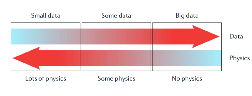
The computational schematic for the general FWI inversion algorithm is illustrated in Figure 1a. This deterministic algorithm is completely physics based and is typically applied to seismic data, as represented on the far left of the spectrum in Figure 2. Here, no data other than the shot gathers are typically used for inversion.

Figure 1: Schematics for data inversion by a) pure-physics FWI, b) pure-data ML, and c) skeletal-data ML where $F({\bf d})$ is a filtering operation that extracts skeletal data from the recorded data. The dashed rectangles indicate that the enclosed system trains on many examples to get the optimal parameters $\mathbf{w}$ that minimize $||{\bf H}_{{\bf w}}{{\bf d}}-{\bf m}^{ML}||^{2}$. The objective functions for each algorithm are on the right.

Figure 2: Diagram illustrating physics-related constraints as a function of data size (Karniadakis et al.,, 2021). Here, physics provides extra information that can make up for the lack of sufficient data in the training of an ML algorithm.

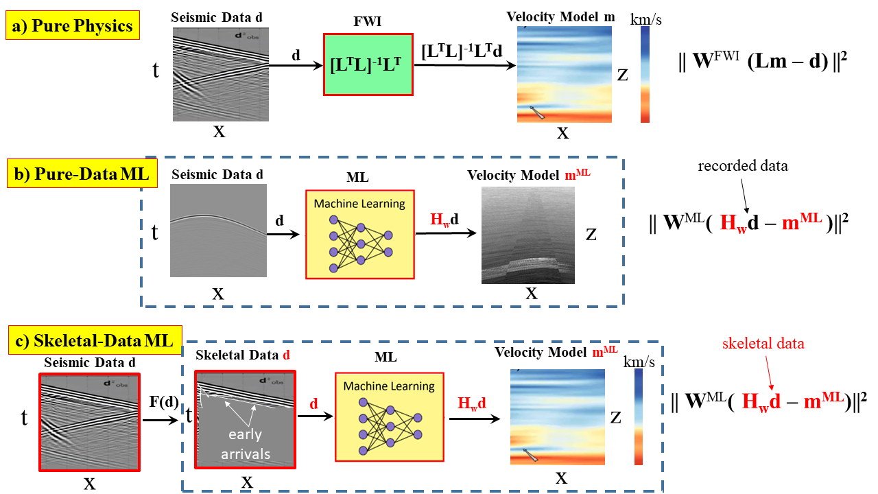
In contrast to FWI, the prediction of a model by a trained neural network (NN) is completely devoid of the explicit constraints of wave-propagation physics. It is an inversion in the sense that the NN parameters ${\bf w}$ are obtained by training to predict the given model ${\bf m}={\bf H}_{{\bf w}}{\bf d}$ from the training pairs $({\bf m},{\bf d})\in training\leavevmode\nobreak\ data$. Here, ${\bf H}_{{\bf w}}$ represents the non-linear operator of the NN, which is a function of the nodal parameters denoted by the vector ${\bf w}$. The ML goal is to find the optimal parameters ${\bf w}^{*}$ that minimize the NN objective function in equation 1 for $\lambda_{2}=0$ (see Figure 1b) s.t.

$${\bf w}^{*} = argmin_{{\bf w}}[\leavevmode\nobreak\ \overbrace{||{\bf W}^{ML}({\bf H}_{{\bf w}}{\bf d}-{\bf m})||^{2}\leavevmode\nobreak\ \leavevmode\nobreak\ +\leavevmode\nobreak\ Regularizer}^{\epsilon^{ML}}\leavevmode\nobreak\ ],$$ (3)

which is typically achieved by a gradient-descent algorithm. Here, ${\bf W}^{ML}$ is the matrix used to optimize convergence such as balancing the number of input classes (Shi et al.,, 2023). Once the network is accurately trained for a generalized set of training pairs, then ${\bf H}_{{\bf w}}$ can be applied to new data to get the associated model.

If the input traces are skeletonized by muting everything but first arrivals then Figure 1c depicts the schematic for skeletal-data ML. Some successful examples that use skeletonized data for training including the inversion of early arrivals in seismic data (Yu et al.,, 2021), recognition of different bird types in pictures of birds Mao et al., (2021) and rock cracks in images of a canyon wall (Shi et al.,, 2023). The case of pure-data NN is represented on the far right of the spectrum in Figure 2, where a huge number of diverse training pairs must be used to accurately estimate the ML model.

The problem with pure-data ML inversion is that it takes an enormous number of training examples to thoroughly train the NN to invert arbitrary test data. Incomplete training, where the training set is limited in its diversity and number of examples, is inevitable for high-dimensional data spaces: increasing the dimension of the data space leads to a shrinkage of the distance between the nearest and farthest data points (Durrant and Kabán,, 2009). This shrinkage can be fatal for inversion methods that use a limited number of diverse training examples. Thus, achieving a marginal improvement in generalizing an NN requires an exponential increase in the number of training examples. As Bishop and Nasrabadi, (2006) states: increasing the input space dimension without enhancing the quantity of available information reduces the model’s power and may give rise to the curse of dimensionality. Fortunately, the problem with incomplete data can be mitigated by using joint inversion to include the constraints of physics, which is a proxy for using new data.

1.1 Joint inversion

Joint geophysical inversion is an approach for simultaneously inverting different types of geophysical data (Vozoff and Jupp,, 1975; Gallardo and Meju,, 2004; Abubakar et al.,, 2012; Zhdanov et al.,, 2021), where the objective function is the summation of regularization terms and misfit functions for each type of data. Typically, the different data sets are recorded by different instruments such as a gravimeter that records the gravity data and geophones that record the seismic data. The density model reconstructed from the gravity data can have structural characteristics similar to the velocity tomogram reconstructed from the seismic data, so a regularization term is added to the misfit function that encourages structural similarities between the gravity and seismic models. As an example, Paulatto et al., (2019) utilized a joint interpretation of seismic and gravity data for characterizing a magma reservoir. Other examples include the inversion of resistivity and traveltime data by Gallardo and Meju, (2004) to image the near surface, and a more comprehensive inversion is by Colombo and De Stefano, (2007) who jointly inverted seismic, gravity, and electromagnetic data for velocity modeling. Juhojuntti and Kamm, (2015) inverted both seismic refraction and resistivity data for imaging the subsurface properties associated with groundwater.

If both a statistical ML method and a physics-based FWI are used to compute a velocity model, then these two methods can be considered different from one another but their final models should agree with one another. To encourage this agreement, their corresponding misfit functions can be added together along with a regularization term to give the joint objective function in equation 1. This joint objective function gives the unifying approach used by physics-informed machine learning (PIML) inversion of geophysical data.

1.2 PIML

To partially overcome the problem of incomplete ML training, Colombo et al., 2021a computed the optimal model $\bf m^{*}$ and weights $\bf w^{*}$ in equation 1 that minimized

$$({\mathbf{w}}^{*},{\bf m}^{*}) = argmin_{{\mathbf{w}},{\mathbf{m}}}[\lambda_{1}||{\bf W}^{ML}({\bf H}_{{\bf w}}{\bf d}^{obs}-{\bf m}^{ML})||^{2}+\lambda_{2}{||{\bf W}^{FWI}({\bf L}{\bf m}-{{\bf d}}^{obs})||^{2}}+$$ (4)

$$\lambda_{3}||{\bf W}^{joint}[{\bf m}-{\bf m}^{ML}]||^{2}+\leavevmode\nobreak\ \leavevmode\nobreak\ Regularizer],$$

where $||{\bf W}^{joint}[{\bf m}-{\bf m}^{ML}]||^{2}$ is a regularizer that softly constrains the FWI and NN models to agree with one another. The weighting matrices ${\bf W}^{ML}$, ${\bf W}^{FWI}$ and ${\bf W}^{joint}$ are selected to optimize convergence and account for noisy data. Here, ${\bf d}^{obs}$ represents the observed data, $\lambda_{i}\leavevmode\nobreak\ i\in[1,2,3]$ are regularization parameters and the optimal solution ${\bf m}^{*}$ can be found, for example, by a gradient-descent method that alternates between solving for the velocity model $\bf m$ and the ML weights ${\bf w}$. Table 1 summarizes four different PIML algorithms which are determined by the values of $\lambda_{i}$ and the selection of the deterministic and NN schemes.

Table 1: PIML algorithms from equation 4, where $(N_{AE},N_{FLI},N_{FWI},N_{it})$ are the number of iterations for the $(autoencoder,\leavevmode\nobreak\ FLI,\leavevmode\nobreak\ FWI,\leavevmode\nobreak\ FWI+ML)$ schemes. The ${\bf Lm}$ represents the finite-difference solution to the wave equation for the velocity model $\bf m$ and ${\bf d^{pred}}={\bf L_{v}}({\bf x},{\bf m^{ML}})$ is the NN solution to the wave equation for the ML velocity model ${\bf m}^{ML}$. The joint regularization function is given by $\epsilon^{const.}=\lambda_{3}||{\bf m}-{\bf m}^{ML}||^{2}$ and the weight matrices have been conveniently neglected.

PIML Type	Schedule	NN Architecture
Skeletal	$(\lambda_{1},\lambda_{2},\lambda_{3})=(1,0,0)$	${\bf H_{w}}$ = Autoencoder
PIML	$for\leavevmode\nobreak\ i=1:N_{AE}$
	$(\lambda_{1},\lambda_{2},\lambda_{3})=(0,1,0)$	$\epsilon^{ML}=\lambda_{1}||{\bf H_{w}}{\bf d^{obs}}-{\bf d^{obs}}||^{2}$;  $\epsilon^{FLI}=\lambda_{2}||{\bf z}^{pred}-{\bf z}^{obs}||^{2}$
	$for\leavevmode\nobreak\ i=1:N_{FLI}$
		${({\bf w^{*}},{\bf z^{*}})}=argmin_{\bf w}=\epsilon^{ML}$, then ${\bf m}^{*}=argmin_{\bf m}\epsilon^{FLI}$
Parallel	$(\lambda_{1},\lambda_{2},\lambda_{3})=(>0,>0,>0)$	${\bf H_{w}}$ = Encoder-Decoder
PIML	$for\leavevmode\nobreak\ i=1:N_{it}$
		$\epsilon^{ML}=\lambda_{1}||{\bf H_{w}}{\bf d^{obs}}-{\bf m^{ML}}||^{2};\epsilon^{FWI}=\lambda_{2}||\overbrace{{\bf d}^{pred}}^{{\bf Lm}}-{\bf d}^{obs}||^{2}$
		$\epsilon=\epsilon^{ML}+\epsilon^{FWI}+\epsilon^{const.}\rightarrow({\bf m}^{*},{\bf w}^{*})=argmin_{\bf m,w}\epsilon$
Iter. Seq.	$(\lambda_{1},\lambda_{2},\lambda_{3})=(0,>0,0)$	${\bf H_{w}}$ = Encoder-Decoder
PIML	$for\leavevmode\nobreak\ i=1:N_{it}$
		${\bf m^{ML}}={\bf H_{w}}{\bf d}^{obs}$; ${\bf d}^{pred}={\bf Lm^{ML}}=\bf{LH_{w}d^{obs}}$
		$\epsilon^{FWI}=\lambda_{2}||{\bf d}^{obs}-{\bf d}^{pred}||^{2}\rightarrow({\bf m}^{*},{\bf w}^{*})=argmin_{\bf w}\epsilon^{FWI}$
	$(\lambda_{1},\lambda_{2},\lambda_{3})=(0,>0,0)$	${\mathcal{L}}=$ PDE; ${\bf H_{w}}\leavevmode\nobreak\ \&\leavevmode\nobreak\ {\bf L_{v}}$ = Fully-Connected NNs
PINN	$for\leavevmode\nobreak\ i=1:N_{it}$
		$\epsilon^{physics}=\lambda_{2}||\mathcal{L}(\overbrace{{\bf L_{v}}({\bf x,m^{ML}})}^{\bf d^{pred}})-{\bf f}||^{2}$; ${{\bf m^{ML}}={\bf H_{w}}{\bf d^{pred}}}$
		$\epsilon^{FWI}=\lambda_{2}||{\bf d}^{pred}-{\bf d}^{obs}||^{2}\rightarrow({\bf m}^{*},{\bf v}^{*},{\bf w}^{*})=argmin_{{\bf v,w}}{\epsilon}^{FWI}$

The PIML algorithm falls in the middle part of the spectrum in Figure 2, where PIML combines physics constraints and training for a subset of the data. Once the ML operator ${\bf H_{w}}$ is trained on a small fraction of the recorded data, then it can be efficiently applied to the rest of the data to get the optimal velocity. This assumes that the test data are similar to the training data.

1.3 Benefits of PIML

There are several potential benefits of PIML compared to standard FWI computed by finite-difference solutions to the wave equation.

1. Empirical tests suggest that PIML algorithms constrained by the physics of wave propagation can sometimes resist getting stuck in a local minima compared to standard FWI.

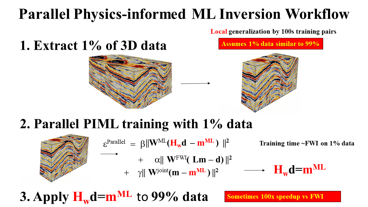
2. Compared to standard FWI, PIML can sometimes provide much faster model estimation of the models associated with the recording site. Instead of training the neural network operator ${\bf H}^{ML}$ on millions of training pairs, the training is only on a small portion, e.g. 1%, of the recorded data as illustrated in steps 1-2 of Figure 3. The velocity models in the training are computed by a traditional FWI code, with the misfit function $||{\bf W}^{FWI}({\bf Lm-d})||^{2}$ as illustrated in step 2 of Figure 3. This training is typically not much more expensive than applying FWI to this reduced data set. If the remaining 99% of the test data ${\bf d}^{test}$ are similar to the trained data, then the trained ${\bf H}^{ML}$ inversion operator can be used to efficiently invert ${\bf d}^{test}$ for the velocity model ${\bf m}\approx{\bf H}^{ML}{\bf d}^{test}$ everywhere below the recording site. This is efficient because applying ${\bf H}^{ML}$ to test data can be more than an order-of-magnitude more efficient than FWI. Training is only performed for a small portion of the recorded data, it is not a global generalization for all types of data. However, the limiting assumption is that the test data should be similar to the trained data, which is a challenge for complex environments.

3. To overcome this limiting assumption one can expensively pretrain a PIML architecture with data recorded over an entire region, and use the trained weights as the starting weights for PIML inversion of new data. This is similar to the strategy of training a large language model (LLM) with millions of training pairs, and then using the trained weights to produce output from new unseen queries. These trained weights can be transfer learned to quickly train the LLM from more detailed information as it becomes available.

Figure 3: Workflow for the parallel PIML inversion of seismic data. The key assumption is that the test data are similar to that of the training data. This approach will likely encounter difficulties when the geology model has rapid velocity changes between different shot locations, such as over salt bodies in the Gulf of Mexico.

1.4 Previous related work

For the geophysical inversion problems, Li et al., (2020) presented a physics-informed method for subsurface property estimation using seismic data, combining full-waveform inversion, subsurface flow processes, and rock physics models, and using automatic differentiation for superior accuracy and performance. Zhu et al., (2021) introduced ADSeismic, a seismic inversion framework that employs reverse-mode automatic differentiation to efficiently calculate gradients. Song and Alkhalifah, (2021) trained a neural network to provide flexible and continuous functional approximations of solutions without matrix inversions, and concludes that PIML’s data-constrained loss function allows it to sometimes reconstruct a wavefield that simultaneously fits recorded data and approximately satisfies the Helmholtz equation. Liu et al., (2023) proposed a differentiable physics model for large-scale joint inverse problems for geologic carbon sequestration monitoring, which utilizes neural networks for model variable reparameterization and forward model implementation. They claim that this approach accurately characterizes subsurface reservoirs, it identifies the migration of CO₂ plume, and it quantifies global parameters that are uncertain in the forward models. They state: … the model can be easily deployed to high-performance computing platforms, thereby providing a computationally efficient approach for large geophysical data. Another approach is by Zhang et al., (2023) who incorporated both seismic data and physical law through regularization of the loss function to estimate velocity and density fields for seismic inversion.

Karniadakis et al., (2021) review some methods where physics constraints are embedded in the ML architecture. In this case, training of the NN does not require modeling of the output by, for example, a standard finite-difference algorithm because the trained NN finds the field values that minimize a loss function that satisfies the associated PDE (Raissi et al.,, 2019). Rotskoff and Vanden-Eijnden, (2020) used a physics-loss function to examine transitions between two metastable states in a high-dimensional probability distribution, incorporating a variational formula for the committor function and a soft penalty on boundary conditions. Patel et al., (2022) developed the control volume physics-informed neural network that expands traditional finite-volume methods to deep learning environments, enabling the estimation of equations of state for shock hydrodynamics models suitable for materials like metals. PIML has also found applications in inverse and ill-posed problems in quantum chemistry (Pfau et al.,, 2020), material sciences (Shukla et al.,, 2020), and molecular simulation (Behler and Parrinello,, 2007).

This paper reviews several approaches to unsupervised PIML inversion of seismic data, where a traditional approach, such as a finite-difference or finite-element method, is used to model the data. We also review the PINN method described by  Karniadakis et al., (2021), where NN architectures are used for both forward and inverse modeling. The goal is to avoid the high computational expense of computing finite-difference solutions to the 3D wave equation. Thus far, this goal has not yet been fully realized and is one of the ongoing efforts in PINN research.

2 Four strategies for PIML

We now present four types of PIML algorithms: skeletal, parallel, iterative-sequential PIML, and the physics-informed neural network (PINN). In the first three cases, a traditional modeling method such as a finite-difference solution to the wave equation is used to estimate the modeled data. The fourth case of PINN, uses NN architectures to perform both forward modeling and inversion of the data. The theory for each method is described, and then numerical results are shown for inverting geophysical data.

2.1 Skeletal PIML inversion

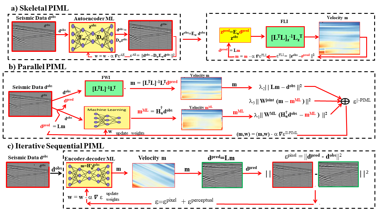
To reduce both the dimension and complexity of the input to a wave-equation inversion algorithm, Chen et al., (2020) and Chen and Schuster, (2020) introduced a hybrid ML and physics-based inversion strategy denoted as Newtonian Machine Learning (NML). Figure 4a illustrates their strategy, where an autoencoder (AE) is trained to condense important features of input seismic traces ${\bf d}_{i}\leavevmode\nobreak\ for\leavevmode\nobreak\ i\in[1,2,...,M]$ into small-dimensional latent vectors ${\bf z}_{i}\leavevmode\nobreak\ for\leavevmode\nobreak\ i\in[1,2,...,M]$. The latent vectors are then inverted for the velocity model by finite-difference solutions to the wave equation, as summarized by the top row of Table 1.

The weights for the AE are defined by

$${\bf w}^{*} = argmin_{{\bf w}}\sum_{i}^{M}||\leavevmode\nobreak\ \overbrace{{\bf H}_{\bf w}{\bf d}_{i}^{obs}}^{predicted\leavevmode\nobreak\ data\leavevmode\nobreak\ \leavevmode\nobreak\ {\bf d}_{i}^{pred}}-{\bf d}_{i}^{obs}\leavevmode\nobreak\ ||^{2},$$ (5)

where ${\bf H}_{\bf w}=\bf D_{\bf w}{\bf E}_{\bf w}$ represents the forward modeling operator of the AE, $\bf E_{\bf w}$ and $\bf D_{\bf w}$ are the respective encoder and decoder operators, and ${\bf w}^{*}$ represents the trained weights of the AE. After training, the $i^{th}$ observed latent vector ${\bf z}_{i}$ associated with ${\bf d}_{i}$ is obtained by

$${\bf z}_{i} = {\bf E}_{{\bf w}^{*}}{\bf d}_{i}\leavevmode\nobreak\ for\leavevmode\nobreak\ i=[1,2,...,M].$$ (6)

We then use forward modeling of the wave equation to produce $M$ predicted traces ${\bf d}_{i}^{pred}$ for a trial-velocity model, which are then used to compute the $M$ predicted latent vectors of low dimension:

$${\bf z}_{i}^{pred} = {\bf E}_{{\bf w}^{*}}{\bf d}_{i}^{pred}\leavevmode\nobreak\ for\leavevmode\nobreak\ i=[1,2,...,M].$$ (7)

The trial-velocity model $\bf m$ is adjusted until all the predicted latent vectors ${\bf z}_{i}^{pred}$ match the observed ones ${\bf z}_{i}$ in a least squares sense. That is,

$${\bf m}^{*} =argmin_{\bf m}\leavevmode\nobreak\ \sum_{i=1}^{M}\overbrace{||\underbrace{{{\bf z}_{i}^{pred}}-{\bf z}_{i}}||^{2}\leavevmode\nobreak\ +\leavevmode\nobreak\ regularization}^{\epsilon^{FLI}},$$ (8)

where ${\bf m}^{*}$ is the optimal velocity model that minimizes the regularized sum of the squared latent-space residuals $\epsilon^{FLI}$. Here, we define $\epsilon^{FLI}$ as the objective function for full latent-vector inversion (FLI). A gradient-descent formula with step-length $\alpha$ is used to iteratively find ${\bf m}^{*}$ s.t.

$${\bf m} \mathrel{\mathop{:}}= {\bf m}-\alpha\nabla_{\bf m}\epsilon^{FLI},$$ (9)

where $\nabla_{\bf m}\epsilon^{FLI}$ is computed using finite-difference solutions to the wave equation (Chen et al.,, 2020; Yu et al.,, 2021). The backpropagation of residuals can be performed by a code that honors the explicit equations of a gradient derived by Chen et al., (2020), or backpropagation of residuals can be computed by automatic differentiation.

Figure 4: a) Skeletal PIML strategy where the autoencoder is trained on a large data set to give the autoencoder parameters $\bf w$ and the low-dimensional vector ${\bf z}$ that skeletonizes the data. The full latent-vector inversion (FLI) algorithm uses solutions to the wave equation to find the optimal velocity model $\bf m$ that minimizes the sum of the squared latent-vector residuals $||{\bf z}^{obs}-{\bf z}^{pred}||^{2}$. b) Parallel PIML strategy where the regularization term $||{\bf W}^{joint}({\bf m}-{\bf m}^{ML})||^{2}$ encourages both the ML velocity model ${\bf m}^{ML}$ and FWI model $\bf m$ to agree in parallel with one another. c) IS-PIML where the ML ${\bf H}_{\bf w}{\bf d}^{obs}$ and wave equation $\bf Lm=d$ modeling operators are sequentially executed because, unlike the parallel PIML strategy, the ML model is equated to the actual velocity model for forward modeling.

In summary, skeletal PIML consists of the two sequential steps described in the top row of Table 1: training of the AE on the observed traces to get the latent-space vectors ${\bf z}_{i}$, then use wave-equation solutions to find the optimal velocity model $\bf m$ that minimizes the sum of the squared latent-vector residuals. The first step is unsupervised AE training and the second step uses the physics of wave propagation to invert for the velocity model. This is equivalent to setting $\lambda_{1}=1$ and $\lambda_{2}=0$ in equation 2 for all of the iterations until convergence. Then set $\lambda_{1}=0$ and $\lambda_{2}=1$ in equation 2, and use the latent variables as the observed data for the FWI objective function. An iterative gradient descent method is then used to find the velocity model that minimizes the z-domain misfit function in equation 9.

2.1.1 Numerical example

As an example, Yu et al., (2021) tested skeletal PIML on refraction data recorded next to the Gulf of Aqaba on the Saudi Arabian peninsula. A 12-lb hammer striking a plate on the ground is used as the seismic source, and each source excitation was recorded by 120 vertical-component receivers placed along a line. The source and receiver spacings are 2.5 m, where each source is excited next to a receiver position.

Yu et al., (2021) used an auotoencoder to reduce the dimension of the input seismic traces, and then inverted a small-dimension latent space vector for the velocity model. The inversion strategy was that of skeletonized inversion which used finite-difference solutions to the wave equation. For comparison, a variety of different methods are used to invert the first-arrival data for the velocity tomograms in Figure 5. The wave-equation traveltime inversion (WT) method is used to compute Figure 5a, where the input windowed data are bandpass filtered peaked at 50 Hz. The starting model is a linear gradient velocity model (Yu et al.,, 2021), and the same data are inverted by the NML method to give the tomogram in Figure 5b.

Figure 5: Top row are tomograms inverted by a) the 50-Hz wave equation traveltime (WT) inversion method (Luo and Schuster,, 1991), b) AE inversion with a 1D latent space and a 50-Hz bandpass filter applied to the data, c) envelope inversion, d) AE inversion with a 2D latent space and e) FWI. Figure from Yu et al., (2021). Below each tomogram are the corresponding first arrivals ${\bf d}^{pred.}$ generated from the tomogram’s velocity model and the associated residual traces ${\bf r}={\bf d}^{pred.}-{\bf d}$ where $\bf d$ represents the recorded trace. Figure adapted from Yu et al., (2021).

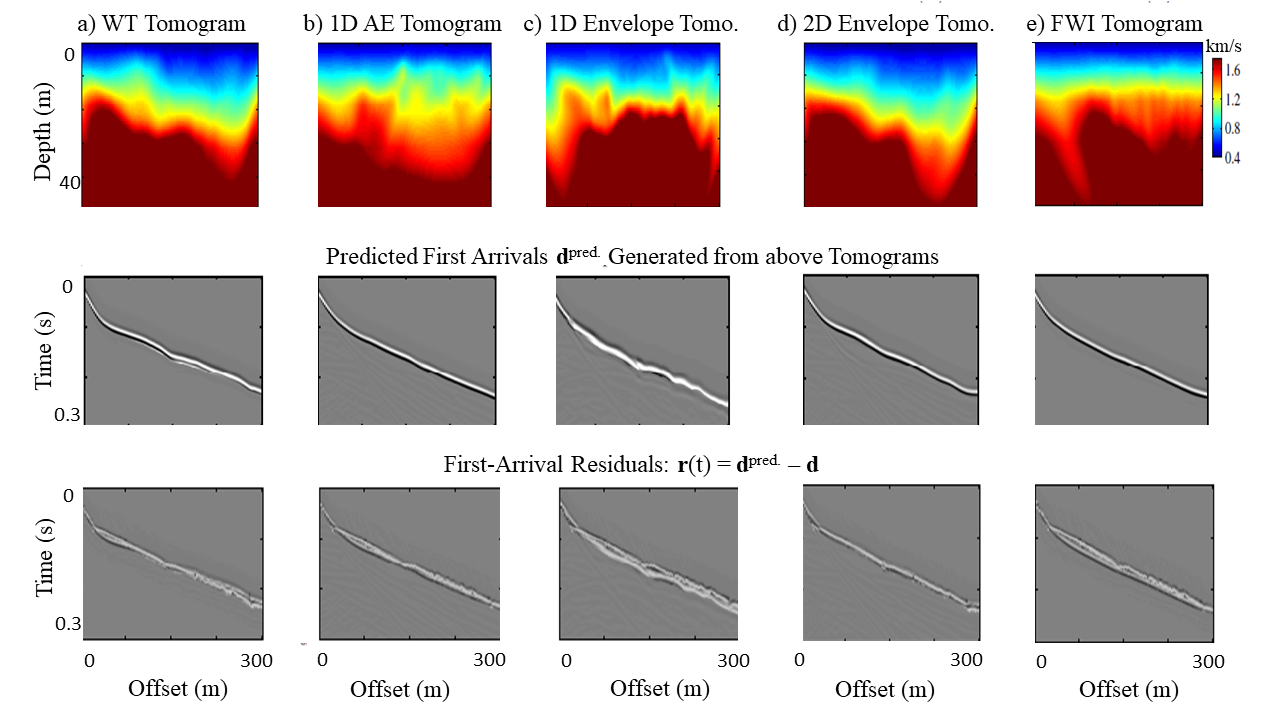
The envelope inversion results are shown in Figure 5c and the FWI tomogram is displayed in Figure 5e. These results were obtained after 20 iterations. The first four inverted tomograms, especially the first and the fourth tomograms in Figure 5a and Figure 5d, suggest the possible location of the Aqaba fault scarp (Hanafy et al.,, 2014) observed on the surface.

The reconstructed early arrivals ${\bf d}^{pred.}$ from each of the tomograms in Figure 5 are displayed in the second row of Figure 5 and are computed by a finite-difference modeling method. Here, the predicted arrivals are subtracted from the actual arrivals to get the residual CSGs in the third row of Figure 5. It is clear that the 2D NML residual in Figure 5 has the smallest residual compared to the other methods.

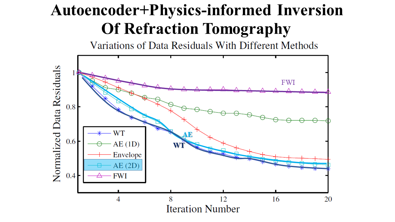
The data misfit curves with the five algorithms are presented in Figure 6. These curves show that the WT and 2D AE methods converge the quickest to a small data residual.

Figure 6: Iteration vs residual for the five algorithms presented in Figure 5. Figures adapted from Yu et al., (2021).

2.2 Parallel PIML inversion

Instead of the skeletal use of ML training followed by a physics-based inversion algorithm, equation 1 and Figure 4b illustrates the parallel minimization (Colombo et al., 2021a, ; Colombo et al., 2021b, ) of the ML and physics-based objective functions in equation 4. Here, the matrices $({\bf W}^{FWI},{\bf W}^{ML})$ are used to downweight unreliable parts of the data or model parameters, and the joint misfit term is used to encourage the ML and physics-driven models to be identical. The positive scalar variables $(\lambda_{1},\lambda_{2},\lambda_{3})$ in the second row of Table 1 moderate the relative importance of the three misfit functions.

A gradient-descent strategy with alternating updates of the ML parameters ${\bf m}^{ML}$ and velocity model ${\bf m}$ can be used to find the optimal velocity model ${\bf m}^{*}$. First, the model ${\bf m}$ is fixed and the parameters for the NN are computed to minimize the objective function $\epsilon^{||-PIML}$ in equation 1. The parameters for the ML algorithm can be initially trained offline on a training set consisting of seismic data and their associated velocity models. This is therefore classified as a supervised learning method. Then the updated ML parameters are fixed and the model ${\bf m}$ is found by gradient descent that minimizes $\epsilon^{||-PIML}$. The term $||{\bf W}^{joint}({\bf m}-{\bf m}^{ML})||^{2}$ encourages agreement between the ${\bf m}$ and ML ${\bf m}^{ML}$ models. This alternating use of the different objective functions is repeated until acceptable convergence. Examples of this procedure for geophysical inversion are presented in Colombo et al., 2021a ; Colombo et al., 2021b . Other physical information, such as seismic faces (Li et al.,, 2021; Zhang and Alkhalifah,, 2022), initial models (Zhang et al.,, 2021), spatial-temporal information (Yang et al.,, 2022), and migration images (Zhang et al.,, 2020), can be also used as the regularization term in the objective function to improve the inversion results. Colombo et al., (2023) also developed a physics-adaptive ML inversion scheme that shows good generalization properties for field applications. Their deterministic inversion scheme is regularized by a penalty term characterized by the difference between the inverted models and ML-predicted models. The resulting models and computed responses are used for augmenting the training data.

Colombo et al., 2021b used the parallel PIML method to invert TEM data. The reconstructed resistivity model is shown in the left column of Figure 7, where the resistivity model obtained by a standard pure-physics algorithm is shown just below it. Both models look similar. However, if the data generated by these models are synthetically computed then the residuals for the parallel PIML model are displayed in the right column of Figure 7 along with those from the standard pure-physics model. It is clear that the parallel PIML results are more accurate than that from standard inversion.

Figure 7: Left column of images compare the results for inverting the resistivity model $\rho({\bf x})$ from TEM data using the parallel PIML method and the standard pure-physics inversion. The residuals of the TEM data are plotted on the right. Figures adapted from Colombo et al., 2021b .

2.3 Iterative-sequential PIML inversion

The parallel PIML ican sometimes require offline training of the ML weights using data and model pairs generated by, for example, synthetic simulations. These simulations should be for models that resemble the actual model that is to be reconstructed from the recorded data. This can be tedious and time consuming for large training sets. To avoid this problem, Jin et al., (2021) developed the unsupervised physics-informed ML inversion method. In this case, the velocity models are obtained by an encoder-decoder network as shown in Figure 4c. Here,

$${\bf w}^{*} = argmin_{{\bf w}}[\overbrace{\sum_{i}^{M}||\leavevmode\nobreak\ {\bf d}_{i}^{obs}-{\bf d}_{i}^{pred}\leavevmode\nobreak\ ||^{2}}^{\epsilon^{pixel}}+\epsilon^{perceptual}\leavevmode\nobreak\ ],$$ (10)

where ${\bf d}_{i}^{obs}$ (${\bf d}_{i}^{pred}$) represents the $i^{th}$ observed (predicted) trace, ${\bf H}_{\bf w}={\bf D}_{\bf w}{\bf E}_{\bf w}$ represents the forward modeling operator of the encoder $\bf E_{\bf w}$ and decoder $\bf D_{\bf w}$ operations, and ${\bf w}^{*}$ represents the trained weights of the encoder-decoder architecture. The perceptual loss $\epsilon^{perceptual}$ objective function is

$$\epsilon^{perceptual} = \sum_{i}(F({\bf d}_{i}^{obs})-F({\bf d}_{i}^{pred}))^{2},$$ (11)

which is used to form the complete objective function

$$\epsilon = \epsilon^{pixel}+\epsilon^{perceptual}.$$ (12)

Here, $F({\bf d}_{i})={\mathbf{z}}_{i}$ is the latent-vector output ${\mathbf{z}}_{i}$ of an encoder network trained on a set of data. These data are those of images and the encoder associated with the training is that of a VGG network (Johnson et al.,, 2016).

Unlike the autoencoder where the input and output are the recorded traces, ${\bf H}_{\bf w}{\bf d}^{obs}=\bf m$ produces the velocity model $\bf m$ from the recorded data ${\bf d}^{obs}$. This velocity model then produces the predicted shot gather ${\mathbf{d}}^{pred}$ shown in Figure 4c, which is obviously in disagreement with the input shot gather ${\bf d}^{obs}$ at the far left. This is because the velocity model generated by the autoencoder is incorrect because its weights $\bf w$ at early iterations do not reproduce a velocity model that predicts the actual data.

A gradient-descent formula

$${\bf w}={\bf w}-\alpha\nabla\epsilon,$$ (13)

is then used to adjust the weights of the encoder-decoder so that a more accurate velocity model ${\bf m}$ is generated in Figure 4c. This computed velocity model is then forward modeled ${\bf d}^{pred}={\bf Lm}$ to get the predicted shot gathers ${\bf d}^{pred}$ by a numerical solution to the wave equation. Repeating these sequential series of steps until $\epsilon$ is minimized defines the IS-PIML method. Some benefits of this method are that it is unsupervised and once it is properly trained, new input data can be quickly inverted by the encoder-decoder to get the velocity model. The third row in Table 1 summarizes these procedures.

In practice, the gradient for small batches in each epoch leads to a lower computational cost than pure physics-based inversion. However, it calculates the data loss through physics-based forward modeling, which leads to a higher cost than the supervised methods (Deng et al.,, 2021).

2.3.1 Numerical example

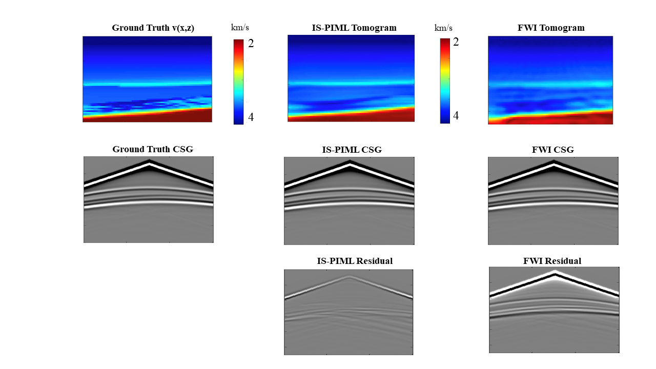
A synthetic data set is used to test the effectiveness of the IS-PIML method. A finite-difference method is used to generate synthetic data from the true velocity model in the left column of Figure 8. These data are inverted to give the IS-PIML and FWI tomograms in the middle and right columns, respectively. A finite-difference method is then used to generate the predicted CSGs using the velocity models from the tomograms, and these predictions are subtracted from the true traces to give the residual traces at the bottom row of Figure 8 (Feng et al.,, 2022). The IS-PIML residuals have noticeably less residual energy compared to the FWI result. In terms of computational cost, the IS-PIML algorithm costs several times more than the FWI for this example.

Figure 8: Comparisons of ground truth velocity model and tomograms (top row), predicted CSGs (middle row) and residuals (the last row) computed by the IS-PIML and FWI algorithms.

2.3.2 Multiphysics PIML

The PIML algorithms can be used to invert for multiple types of data, each governed by a different type of physics. This can be done by creating a joint objective function by regularizing and summing together weighted objective functions associated with each type of data. Typically, the regularization function enforces a soft constraint that equates one type of model with the other one.

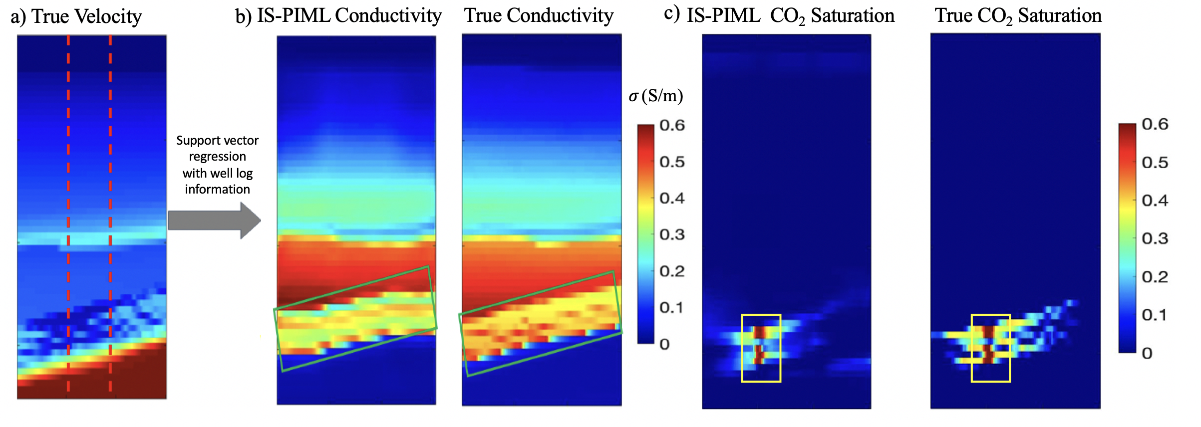
For example, consider the seismic velocity model in Figure 9a where the dashed red lines correspond to well locations. Conductivity logs $\sigma(z)$ and $CO_{2}$ saturation logs $s(z)$ are recorded and are correlated to the velocity tomogram at each depth using a support regression algorithm (Feng et al.,, 2022). This gives the mapping between the seismic velocity values and the conductivity $F(v(x_{well},z))=\sigma(z)$ and $CO_{2}$ saturation $G(v(x_{well},v(z))=s(z)$ values, where $v(x_{well},z)$ is the vertical velocity profile of the tomogram at the well offset $x_{well}$. These functions $F(v)$ and $G(v)$ are used to map the 2D tomogram velocity $v(x,z)$ to the pseudo-conductivity $\sigma(x,z)$ and the pseudo-CO₂ saturation. With the pseudo labels, the iterative sequential-PIML methodology gives predicted conductivity and CO₂ saturation in Figure 9band 9c. Both images compare well to the true conductivity and CO₂ saturation images.

Figure 9: a) Well logs denoted by red dashed lines, b) IS-PIML predicted and true conductivity. c) IS-PIML predicted and true CO₂ saturation.

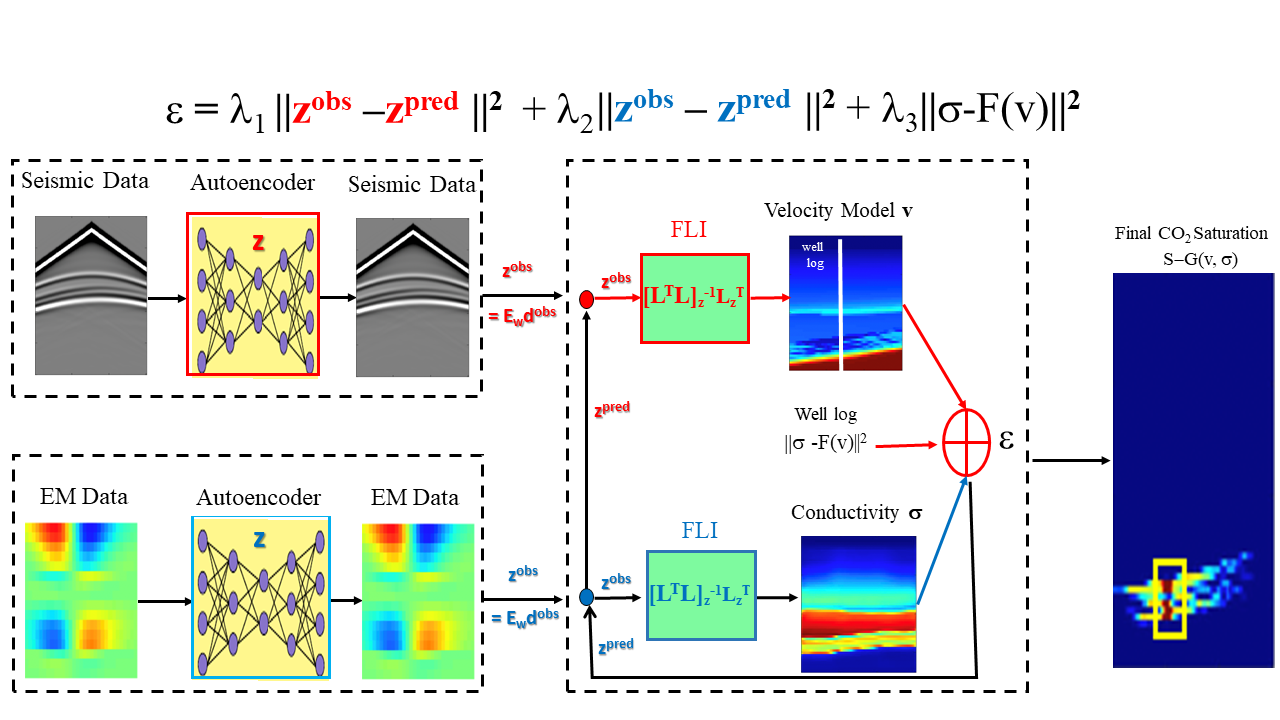
The sequential PIML can also be used to combine models from different types of data and well-log information to obtain models constrained by well-log information. Figure 10 provides an example of this for electromagnetic (EM) and seismic data to estimate the pseudo-saturation image. The joint objective function at the top is a combination of FLI misfit functions and the well-log constraint.

Figure 10: Hypothetical schematic for multiphysics sequential PIML where electromagnetic (EM) and seismic are skeletalized to latent vectors $\bf z$, and the output consists of conductivity and velocity images inverted by FLI. These images are constrained by the mapping $\sigma=F(v)$ between conductivity and velocity obtained from well-log information. The saturation mapping from conductivity and velocity values is also obtained from well logs to get $S=F(c,\sigma)$, which is used to get the CO2 saturation image on the right.

2.4 Physics-informed neural network

The previous sections showed different ways of combining an objective function computed by a NN and one computed using a finite difference solution to the wave equation. Now we introduce a physics-informed neural network (PINN) that only uses NN architectures to compute both the forward modeling solution to the wave equation as well as its inverse solution (Raissi et al.,, 2019; Karniadakis et al.,, 2021). The hypothetical advantage is that PINN can hopefully avoid the large computational expense of finite-difference modeling of 3D data, with the possible penalty of reduced accuracy. This goal has not yet been fully met, and it is too early to judge the practical benefits of PINN compared to FWI in inverting seismic data (Gholaminejad,, 2022). The PINN schematic for inverting data can be represented by the IS-PIML schematic in Figure 4c, except the forward modeling operator $\bf L$ is now computed by a trained NN rather than a FD solution to the wave equation.

Appendix I describes how PINN solves the forward problem by an NN, and then explains the strategy for inverting for model parameters from recorded data. Examples for modeling and inverting synthetic data by a NN are described in the next section, and the PINN algorithm is summarized in the last row of Table 1.

2.4.1 Examples of inverting seismic data by PINN

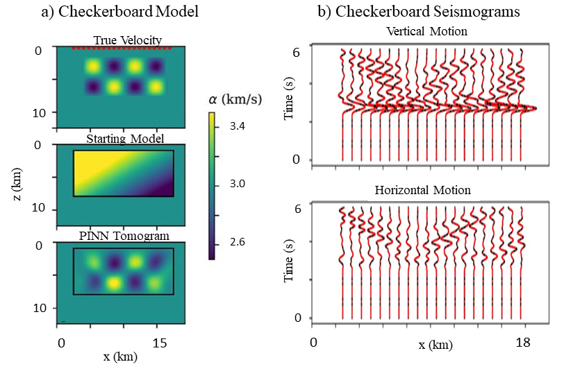
The checkerboard velocity model in Figure 11 is used to demonstrate PINN inversion of acoustic data for the velocity model. Here, the true velocity model is shown at the top of (a), the starting model is in the middle of (a) and the bottom image is the tomogram inverted by PINN (Rasht-Behesht et al.,, 2022). The tomogram and the actual model largely agree with one another.

In this example, there are 20 evenly-spaced seismometers (red squares) along the top of the model and there are nine-point sources evenly distributed at a depth of 10 km, each having a Gaussian wavelet with a dominant frequency of 20 Hz and the recording time is 5 s. Therefore, this example resembles that for a crosswell experiment with horizontal source and receiver wells. The free surface boundary condition for this simulation was not enforced.

The NN consists of 10 layers, each with 100 neurons per layer. There are 11600 total samples in all of the recorded seismograms, and the training data for the PDE and early-arrival snapshots consist of 60,000 and 3,600 points respectively. There are two early time snapshots (at $t=0$ and $t=0.05\leavevmode\nobreak\ s$) in the training data, and they are used as enforced data constraints that get information about the background velocity. There is a typo in the Rasht-Behesht et al., (2022) paper, and the author (Huber, pers. comm.) states that the data residual in the loss function is actuated and the sources are at a depth of 10 km.

The actual and predicted seismograms in Figure 11b) mostly agree with one another. The physics loss term is computed on a set of randomly selected training points $(x_{1},x_{2},t)$, and the loss term associated with two early snapshots is weighted by a factor that is 10 times more than the physics loss term.  Rasht-Behesht et al., (2022) state that the current state-of-the-art PINNs provide good results for the forward model, even though spectral element or finite-difference methods are more efficient and accurate.

Figure 11: (a) True velocity, starting velocity and inverted velocity models (aka tomogram), and (b) corresponding predicted and true seismograms recorded along the top of the model. The blue lines are the true seismograms computed by a type of a finite-element method and the red dashed lines are computed by the PINN.

Some recent improvements that improve the performance of PINN include the following.

1. Adaptive activation function. The $\tanh(x)$ activation sometimes fails to capture high-frequency solution modes, so it is replaced by an adaptive activation function such as $\tanh(\alpha x)$ or $max(0,\alpha x)$, where $\alpha$ is a learnable parameter for each layer. This can help capture finer details in the predicted data and the model. Empirical results suggest that the siren function $\sin(x)$ can sometimes be even more effective in capturing finer details. Employing periodic activation functions also increased the effectiveness in predicting pressure and solute concentration fields in heterogeneous porous media (Faroughi et al.,, 2022).

2. Dynamic weighting of the loss functions.  Wang et al., (2021) observed that the NN gradient for the gradient tends to favor satisfying the physics equations at the expense of largely ignoring the data and boundary constraints. Thus, the loss functions should be weighted to better balance the data terms for unbalanced constraints. For example, the scalar weight $\lambda_{boundary}$ for the boundary loss term $\lambda_{boundary}\epsilon^{BC}$ should be much greater than that for the physics term $\lambda_{physics}\epsilon^{physics}$ if it is weighted as

   $$\lambda_{boundary} = \frac{|\nabla_{\theta}\epsilon^{physics}|}{|\nabla_{\theta}\epsilon^{BC}|},$$ (14)

   because $|\nabla_{\theta}\epsilon^{BC}|$ is often much smaller than $|\nabla_{\theta}\epsilon^{physics}|$ for most inputs into an NN layer; here, $\theta$ represents the NN parameters. Another approach is to identify which types of training data are harder to train and force the NN to focus on those data before training the next step Li and Feng, (2022).

3. Random distributions of points in time and space are more effective than a uniform gridding. The density of points should be increased where the physics loss is high (Yu et al.,, 2021).

4. A quasi-Newton L-BFGS is more effective than an SGD approach.

5. Huang and Alkhalifah, (2022) claim that, compared to the commonly used PINN with random initialization, their frequency upscaling approach exhibits notable superiority in terms of convergence and accuracy with a two-hidden-layer model.

6. Sun et al., (2023) used the PIML approach to invert synthetic seismic data. Instead of using a ML method for their forward modeling, they used a standard finite-difference solver so that their scheme can be described by the IS-PIML schematic in Figure 4c. Their empirical results showed that the PIML inversions were largely resistant to getting stuck in a local minimum compared to the standard FWI approach for poor starting models. See Figure 12. They also found that replacing the ReLu functions with sine-based activation functions speeded up convergence by more than an order of magnitude. However, the reconstructed models from PIML appeared to be less accurate compared to FWI tomograms when significant amounts of random noise were added to the data (see Figure 13). They claimed that their approach ”exhibits a strong capacity for generalization, and is likely well-suited for multi-scale joint geophysical inversion.”.

   

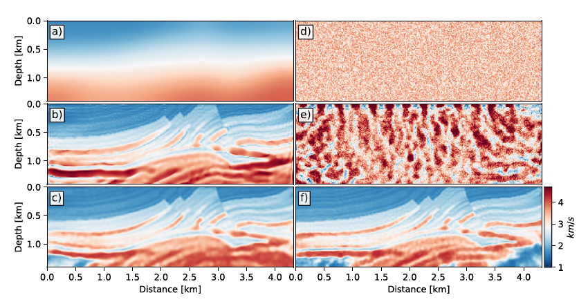
   Figure 12: The first row of images depicts the a) smooth and d) random initial-velocity models. From left to right, the second row depicts the tomograms obtained by FWI for the smooth and random starting models. The third row is the same except these tomograms are computed by the PIML inversion in Sun et al., (2023) These images from Sun et al., (2023) suggest that PIML inversion is somewhat resilient to poor starting models.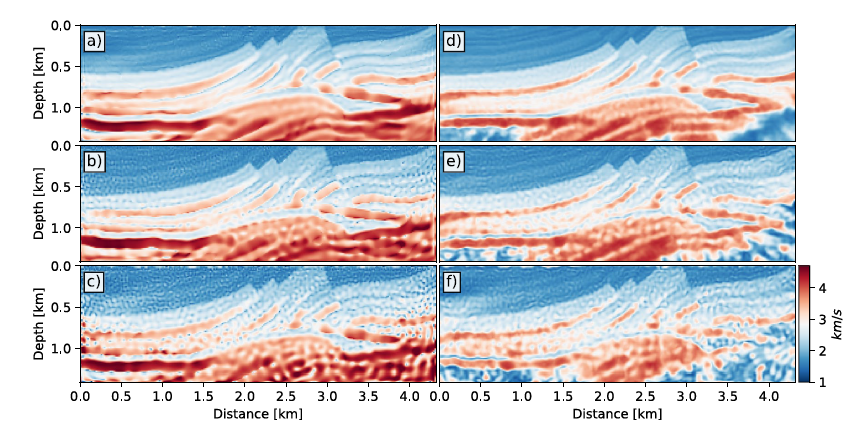

   

   Figure 13: The first row of images depict the tomograms inverted by a) FWI and d) PINN from the noise-free data and a good starting model. From left to right, the second row depicts the tomograms computed by the b) FWI and e) PINN methods where the input data have additive random noise with $\sigma=2\sigma_{0}$. The third row is the same except the input data are twice as noisy with $\sigma=4\sigma_{0}$. These images from Sun et al., (2023) suggest that PIML inversion is somewhat more sensitive to noisy data than FWI.

3 Summary

We overviewed four types of PIML strategies that combine an ML algorithm with a physics-based inversion strategy. The first three require solutions to the wave equation using a standard solver such as the finite-difference or finite-element methods. The last one, denoted as PINN, only requires a neural network to find the solutions to the governing equations and the model parameters.

1. Skeletal PIML is an unsupervised method that reduces the dimension of the data to the latent-space variables, and then a physics-based inversion inverts them to estimate the optimal model. Dimensional reduction of the data often reduces the chances of getting stuck in a local minimum, but at the possible cost of losing some resolution. There is no need for supervision or for estimating the regularization values because of the sequential one-and-done nature of each algorithm. The unsupervised autoencoder of Ladjal et al., (2019) is a non-linear generalization of the linear principal component transform (PCT), where the singular vectors with the largest singular values are similar to the latent vectors from an autoencoder. Their PCT autoencoder projects data to and from the lower-dimensional subspace so that the latent-space components (axes) are ordered in terms of decreasing importance and each component of a code is statistically independent from the other components.

2. The parallel PIML strategy is to train the ML algorithm and the physics-based algorithms in parallel reconstruct both ${\bf m}^{ML}$ and $\bf m$, and use the penalty term $||{\bf m}-{\bf m}^{ML}||^{2}$ to bring the models into agreement with one another. The starting weights for the ML architecture can be trained with labeled data, and then retrained with the parallel PIML procedure for new data. Once the ML algorithm is sufficiently trained then using ${\bf m}^{new}={\bf H_{w}}{\bf d}^{new}$ to get the new model ${\bf m}^{new}$ from new data ${\bf d}^{new}$ is typically much less costly than that from a physics-based inversion algorithm. The assumption is that ${\bf m}^{ML}$ is close enough to the global minima so that its neighborhood can be explored by the physics-based gradient algorithm to quickly find the global minimum. Determining the optimal values of the regularization parameters is an active area of research.

3. Iterative-sequential PIML is an unsupervised method where the output of the ML model ${\bf m}^{ML}$ model is used to generate the input data ${\bf d}^{pred}$. This $k^{th}$ iterate data is used to generate a data misfit function $||{\bf d}-{\bf d}^{pred}||^{2}$, which is then minimized by updating the ML weights by a gradient-descent method. Once the IS-PIML is trained, then the trained ML portion of the algorithm can be used to efficiently predict models from new data.

   Empirical tests suggest that constraining the ML algorithm to honor the physics of the data can sometimes yield more efficient and accurate reconstructions of earth models compared to pure ML-based inversion. Another benefit is that the PIML training time for the ML algorithm can sometimes require less computational effort compared to standard ML that only uses data for training. This trained ML architecture can then be used to economically invert for models from new data ${\bf d}$ compared to standard FWI. Such data can be recorded over geology similar to that of the training data or include many more unused seismic lines from the same survey. Another benefit is that some PIML algorithms do not require labeling of the training data, which can be a big advantage for large data sets. Improving the robustness, convergence speed, and accuracy of these hybrid PIML strategies is an active area of research.

4. The PINN strategy does not require a standard finite-element or finite-difference solver to compute solutions to the wave equation, or its inverse. It only requires a neural network, where the optimal loss function satisfies the PDE, boundary+initial conditions, and recorded data. Results so far suggest that PINNs can accurately find solutions to the wave equation for smooth velocity models. However, many more epochs are needed to find wavefield solutions for complex velocity models. Thus far, PINNs are not more efficient than standard solvers for general velocity models. However, if the solutions to a large number of velocity models are needed, then solutions by a trained PINN are claimed to be more efficient than those from a standard solver. This assumes that the models are similar to one another. One strategy is to use the trained weights from a modest number of models to be the initial weights for training the NN for other models.

   It is too early in its development to state that inversion of the velocity model by PINNs is more effective and efficient than standard FWI. Nobody has come close to demonstrating this claim. There are many problems to overcome, including the low accuracy and slow convergence with complex velocity models, optimal selection of the network size, the weighting of the misfit functions, choice of network architecture, data size, step length, type of gradient descent method, and many other issues.

If the PIML approach is ever to replace standard FWI then it must be an order-of-magnitude faster, be just as accurate, and be just as robust with noisy and incomplete data as FWI. Thus far, this goal has not yet been achieved. However, if the NN modeling and inverse operators are expensively pretrained to be generalized for data recorded over a large geographic region, then the trained weights can be transfer learned to expedite the PIML inversion of new data collected in the trained region. For example, a general PIML can be pretrained with 3D data over many data examples recorded in the Ghawar region of Saudi Arabia. These weights can then be used for PIML inversion of time-lapse data or new data recorded in that region. This assumes that the NN operations are much more efficient than that of standard FWI, which is almost always the case.

This goal of pretraining a PIML architecture with data recorded over an entire region is similar to the strategy of training a large language model (LLM), and then using the trained weights to produce output from new unseen queries. These weights can be transfer learned to quickly train the LLM from more detailed information as it becomes available.

4 Appendix I: Forward and Inverse Modeling by PINN

This appendix first explains forward modeling by PINN. The next section describes both the forward modeling and inversion methods using PINN.

4.1 Forward modeling by PINN

To avoid the finite-difference modeling of the velocity model, Raissi et al., (2019) and Karniadakis et al., (2021) introduced the PINN approach that uses the partial differential equations of the governing equations as a constraint to the NN system. If $\mathcal{L}u=f$ represents the PDE applied to the scalar field $u$ and $f$ is the localized source function, then the loss function is defined as the sum of the squared residuals

$$\epsilon^{PINN} = \sum_{i\in{\mathcal{D}}}(\mathcal{L}u_{i}-f_{i})^{2}+{regularization},$$ (15)

where the summation is over the points in the entire computational domain $\mathcal{D}$ and the regularization term includes the constraints imposed by the recorded data, the boundary conditions and the initial conditions.

Let us use a simple example to demonstrate the PINN method. Here we use the 2D elliptic equation

$$\overbrace{-\nabla\cdot a({\bf x};\nu)\nabla u({\bf x};\nu)+c({\bf x})u({\bf x};\nu)}^{\mathcal{L}} = f({\bf x}),$$

$$u=0,\leavevmode\nobreak\ \forall x_{1}=1;\leavevmode\nobreak\ u=1,\leavevmode\nobreak\ \forall x_{1}=0;\leavevmode\nobreak\ \frac{\partial u}{\partial n}=0,\leavevmode\nobreak\ \leavevmode\nobreak\ \forall x_{2}=0,$$ (16)

where $\nu$ is a random variable associated with the model parameter function $a({\bf x};\nu)$. Figure 14a depicts the computational domain as a 2D unit box where $0\leq x_{1}\leq 1$, $0\leq x_{2}\leq 1$, where the boundary conditions on the left and right sides are $u(0,x2)=0$ and $u(1,x2)=1$, respectively. The boundary condition on the bottom of the box at $x_{2}=0$ is $\partial u/\partial n=0$ and the source function is imposed upon the top of the box at $x_{2}=1$. Each selection of $\nu$ leads to a different parameter model as depicted by the colored images in Figure 14a.

Figure 14: a) Random distribution of parameter models, b) input of boundary conditions along the sides of the model and the source distribution $f({\bf x})$ along the top, c) the neural network architecture and loss function $\epsilon^{physics}$, and d) output field values $u({\bf x};\nu)$ in the interior of the model are used to form the loss function $\epsilon$ as the single scalar output. The gradient $\nabla_{\bf w}\epsilon^{physics}$ can be computed by automatic differentiation of the NN.

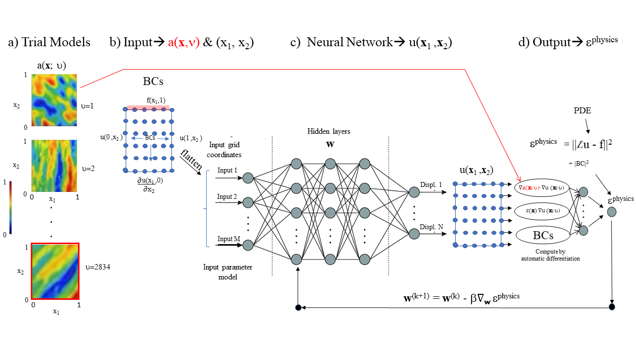
The NN architecture is depicted in Figure 14, where the loss function $\epsilon^{physics}$ is given by

$$\epsilon^{physics} = \overbrace{<\sum_{{\bf x}_{i}\in V}\{-\nabla\cdot a({\bf x}_{i};\nu)\nabla u({\bf x}_{i};\nu)+c({\bf x}_{i})u({\bf x}_{i};\nu)-f({\bf x}_{i})\}^{2}>_{\nu}}^{PDE}$$ (17)

$$+\overbrace{<\sum_{{\bf x}_{i}\in\Omega_{1}}u({\bf x}_{i})^{2}+\sum_{{\bf x}_{i}\in\Omega_{2}}\{\frac{\partial u({\bf x}_{i})}{\partial n}\}^{2}>_{\nu}}^{BC},$$

where the term $<\leavevmode\nobreak\ \leavevmode\nobreak\ >_{\nu}$ indicates averaging over the distribution of random parameter models as a function of the random variable $\nu$. Here, ${\bf x}_{i}\in V$ denotes the set of points in the interior of the model, ${\bf x}_{i}\in\Omega_{1}$ denotes the set of boundary points with Dirichlet boundary conditions, and ${\bf x}_{i}\in\Omega_{2}$ denotes the set of boundary points with Neumann boundary conditions. The NN produces output field values throughout the 2D domain in Figure 14c, where the NN is trained on batches of different input parameter models until the loss function is minimized. The remarkable property here is that the ground truth field values $u({\bf x};\nu)$ do not need to be computed by a finite-difference algorithm, they are computed by the NN. An automatic differentiation method can be used to compute their spatial derivatives $\nabla u$ in the loss function of equation 17; alternatively, a finite-difference approximation can be applied to the $u({\bf x};\nu)$ computed by the NN to get the spatial derivatives. The weights and biases of the NN are computed by, typically, an Adam gradient descent method where the residual is back-propagated by automatic differentiation. Minimizing the loss function ensures that the PDE is satisfied to some specified tolerance.

Minimizing the loss function does not always guarantee convergence to a global minimum, so the Dirichlet principle (Karumuri et al.,, 2020) can be used to provide a robust loss function given by

$${\mathcal{L}}(\theta) = <\sum_{i\in D}\{\frac{1}{2}a({\bf x}_{i})\nabla\tilde{u}({\bf x}_{i};\nu,\theta)+c({\bf x}_{i})\tilde{u}^{2}({\bf x}_{i};\nu,\theta)-f({\bf x}_{i})\tilde{u}({\bf x}_{i};\nu,\theta)\}+\sum_{j\in\Omega_{1}+\Omega_{2}}g_{N}\tilde{u}({\bf x}_{j};\nu,\theta)>_{\nu},$$

where the last summation is over the boundary points of the parameter model and $g$ denotes the appropriate operation for the boundary condition. We now include a tilde over the displacement function $u$ to indicate that it is computed by the NN with the unknown NN parameters $\theta$.

Karumuri et al., (2020) used equation LABEL:Inv.FWI.ML.eq4 to train an NN by the PINN procedure using several hundred input parameter models. After training, an input parameter model is shown in Figure 15a, and the ground truth displacement field computed by a finite-volume method (FVM) is depicted in Figure 15b. The output displacement field computed by the trained NN is shown in Figure 15c where there are some discrepancies between it and the ground truth image in Figure 15b. The low-wavenumber features are accurately computed, but the fine details of the NN solution are in error. There are at least two causes for these errors: spectral bias and vanishing gradients.

Figure 15: (a) Input parameter model, (b) output $u(x_{1},x_{2})$ of finite-volume modeling (FVM), and (c) output $u(x_{1},x_{2})$ of the neural network. Images adapted from Karumuri et al., (2020).

The spectral bias problem (Rahaman et al.,, 2019) is similar to the multiscale problem in FWI: low-wavenumber features converge more quickly with iterative FWI, while it takes many more iterations for the solution to converge to the high-wavenumber features of the model. The partial solution to this problem is to use Fourier features (Rahaman et al.,, 2019; Tancik et al.,, 2020), which transforms the effective neural tangent kernel into a stationary kernel with a tunable bandwidth.

There is debate as to the advantages of PINNs for forward modeling compared to the standard modeling methods of finite elements or finite differences. For modeling in solid mechanics, Haghighat et al., (2021) state that their experience so far suggests that PINN as a forward solver does not lead to advantages in either accuracy or performance.

However, Haghighat et al., (2021) point out the advantage of PINNs when the PINN is expensively trained on data and known models, but new data associated with similar models need to be simulated by PINNs. In this case, the weights of the previously trained models are used with transfer training as the initial weights for the PINNs, and the new data are efficiently modeled by PINNs. The authors state that the advantage of deep learning and PINNs is that a trained PINN is much less costly to execute than classical methods that rely on forward simulations. They demonstrate this advantage by making small perturbations of the model parameters, i.e. changing $\lambda$ and $\mu$ values, to assess the sensitivity of the data to changes in the model parameters. Recycling trained weights to act as initial weights for new models is similar to the frequency-upscaling approach by Huang and Alkhalifah, (2022) for forward modeling of the Helmholtz equation. Here, they used the NN weights trained for low-frequency sources as initial NN weights for modeling the wavefields initiated by high-frequency sources. This frequency-scaling is similar to the multiscale approach used for FWI (Bunks et al.,, 1995) where low-pass filtered data are first inverted for a velocity model, which is then used as the starting model for data with higher frequencies.

Training of the elastic data is tested with a number of different approaches. In this regard, Haghighat et al., (2021) state the following. There are three ways to train the network: (1) generate a sufficiently large number of datasets and perform a one-epoch training on each dataset, (2) work on one dataset over many epochs by reshuffling the data, and (3) a combination of these. When dealing with synthetic data, all approaches are feasible to pursue. However, strategy (1) above is usually impossible to apply in practice, especially in space, where sensors are installed at fixed and limited locations. In the original work on PINN (Raissi et al.,, 2019), approach (1) was used to train the model, where datasets are generated on random space discretizations at each epoch. Here, we follow approach (2) to use training data that we could realistically have in practice.

4.2 Inverse problem by PINN

The seismic inverse problem in the marine case is defined as finding the velocity model that is forward modeled to compute the predicted pressure field $p({\bf x},t)$ that honors the acoustic wave equation

$$[\nabla^{2}-\frac{1}{c({\bf x})^{2}}\frac{\partial^{2}}{\partial t^{2}}]p({\bf x},t) = f({\bf x},t),$$ (19)

and agrees with the observed seismograms $p({\bf x}_{h},t;{\bf x}_{s})^{obs}$ recorded along an evenly sampled line of hydrophone locations ${\bf x}_{h}$ denoted by the set of points ${\bf x}_{h}\in{\mathcal{D}}_{data}$. We will assume a 2D model and hydrophones that are fixed either along the ocean floor or just below the free surface. Here, $c({\bf x})$ is the acoustic velocity in the ocean-earth model and $f({\bf x}_{s},t)$ represents a point source at ${\bf x}_{s}$ excited along an evenly spaced line of points ${\bf x}_{s}\in\mathcal{D}_{src}$, where each source is excited by a bandlimited wavelet $w(t)$. The hydrophone line records the pressure fields excited by each source and is below and parallel to the line of source locations at ${\bf x}_{s}\in{\mathcal{D}}_{src}$. The boundary condition on the ocean’s surface is $p(x_{1},x_{2}=0,t)=0\leavevmode\nobreak\ \leavevmode\nobreak\ \forall x_{1}$ and all-time samples $0\leq t\leq T$. The bottom and sides of the model have absorbing boundary conditions (Yilmaz,, 2001).

Agreement between the observed $p({\bf x}_{i},t_{k};{\bf x}_{j})^{obs}$ and NN predicted $p({\bf x}_{i},t_{k};{\bf x}_{j})$ seismograms is defined as the velocity model that minimizes the sum of the squared residuals:

$$\epsilon^{data} = \frac{1}{M_{D}}\sum_{{\bf x}_{i}\in{\mathcal{D}}_{data}}\sum_{{\bf x}_{j}\in{\mathcal{D}}_{src}}\sum_{t_{k}\in{\mathcal{D}}_{time}}(p({\bf x}_{i},t_{k};{\bf x}_{j})-p({\bf x}_{i},t_{k};{\bf x}_{j})^{obs})^{2},$$ (20)

where ${\mathcal{D}}_{data}$ represents the set of hydrophone locations just below the free surface, ${\mathcal{D}}_{time}$ is the set of time samples, and $M_{D}$ is the total number of sampled points in the summand. The objective function for computing the pressure field that satisfies the acoustic wave equation by an NN is defined as

$$\mathcal{\epsilon}^{physics} = \frac{1}{M_{p}}\sum_{{\bf x}_{j}\in{\mathcal{D}}_{src}}\sum_{{\bf x}_{l}\in{\mathcal{D}}_{model}}\sum_{t_{k}\in{\mathcal{D}}_{time}}\{\overbrace{[\nabla^{2}-\frac{1}{c({\bf x}_{l})^{2}}\frac{\partial^{2}}{\partial t^{2}}]}^{{\mathcal{L}}}p({\bf x}_{l},t_{k};{\bf x}_{j})-f({\bf x}_{j},t_{k})\}^{2};$$

where ${\mathcal{D}}_{model}$ is the set of sampled points in the velocity model and $M_{p}$ is the total number of sampled points in the summand.

The boundary conditions on the free surface and the absorbing boundary conditions, are included in

$$\epsilon^{BC} = \frac{1}{M_{BC}}\sum_{i\in{\mathcal{D}}_{boundary}}|A_{i}|^{2},$$ (22)

where $A_{i}$ represents the boundary conditions associated with all the points on the boundary and all the time samples, ${\mathcal{D}}_{boundary}$ represents the set of indices associated with these samples, and $M_{BC}$ is the total number of boundary samples in both time and space. For example, the boundary conditions might take on the following form:

$$Left\leavevmode\nobreak\ ABC: \leavevmode\nobreak\ \leavevmode\nobreak\ \frac{\partial p({\bf x},t)}{\partial t}-\frac{1}{c({\bf x})}\frac{\partial p({\bf x},t)}{\partial x_{1}}=0,\leavevmode\nobreak\ {\bf x}=(x_{1}=0,x_{2})\leavevmode\nobreak\ for\leavevmode\nobreak\ 0\leq x_{2}\leq 1,$$

$$Right\leavevmode\nobreak\ ABC: \leavevmode\nobreak\ \leavevmode\nobreak\ \frac{\partial p({\bf x},t)}{\partial t}+\frac{1}{c({\bf x})}\frac{\partial p({\bf x},t)}{\partial x_{1}}=0,\leavevmode\nobreak\ {\bf x}=(x_{1}=1,x_{2})\leavevmode\nobreak\ for\leavevmode\nobreak\ 0\leq x_{2}\leq 1,$$

$$Bottom\leavevmode\nobreak\ ABC: \leavevmode\nobreak\ \leavevmode\nobreak\ \frac{\partial p({\bf x},t)}{\partial t}+\frac{1}{c({\bf x})}\frac{\partial p({\bf x},t)}{\partial x_{2}}=0,\leavevmode\nobreak\ {\bf x}=(x_{1},x_{2}=1)\leavevmode\nobreak\ for\leavevmode\nobreak\ 0\leq x_{1}\leq 1,$$

$$Free\leavevmode\nobreak\ Surface: \leavevmode\nobreak\ \leavevmode\nobreak\ p({\bf x},t)=0,\leavevmode\nobreak\ {\bf x}=(x_{1},x_{2}=0)\leavevmode\nobreak\ \leavevmode\nobreak\ for\leavevmode\nobreak\ 0\leq x_{1}\leq 1,$$ (23)

where $c$ takes on the velocity near the boundary point of interest. The source wavelet $w(t)$ turns on shortly after $t=0$ to excite the model. The initial conditions can be enforced by setting $p({\bf x},t)$ and $\frac{\partial p({\bf x},t)}{\partial t}=0$ at $t=0$ $\forall{\bf x}$ with the loss function denoted as $\epsilon^{IC}$.

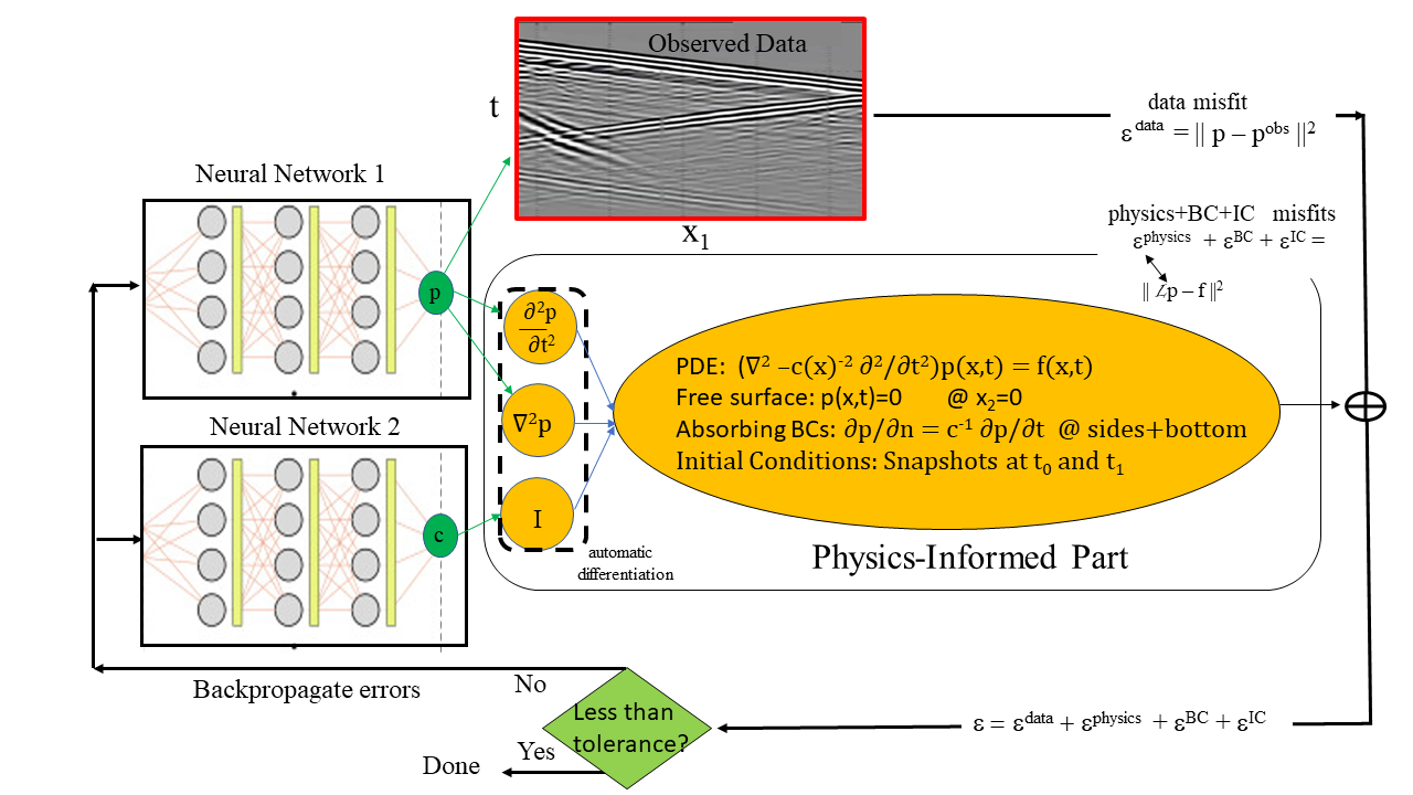
Therefore, the inverse PINN objective function $\epsilon$ is the combination of the objective functions in equations 20-22 and $\epsilon^{IC}$:

$$\epsilon^{PINNi} = \epsilon^{data}+\epsilon^{physics}+\epsilon^{BC}+\epsilon^{IC}+regularization,$$ (24)

where the schematic description is in Figure 16.

Figure 16: Workflow for inversion of seismic data by PINN using the objective function in equation 24. A pass through the data loss term is carried out with a batch of data, and then its output is used to carry out a pass through the physics loss term. Adapted from Rasht-Behesht et al., (2022).

The spatial and temporal grids do not have to be evenly sampled, and are often sampled at random points both in space and time. This suggests that some cost savings can be made by reducing the number of points at which the PDE must be solved. However, the low-frequency details appear to lead to faster convergence than the higher-frequency details. This suggests that a multiscale approach should be useful, where low-frequency data is first inverted, and the low-wavenumber model and PINN weights (via transfer learning) are used as the starting model for the next higher-frequency data. Another possibility is to use the low-wavenumber inverted model as the starting model for standard FWI (Song and Alkhalifah,, 2021). Muller et al., (2022) use transfer training from low-wavenumber models and simple data to capture the main velocity trend of the actual model. They used PINN to stabilize the inversion, acting like a regularizer and avoiding local minima-related problems.

References

- Abubakar et al., (2012) Abubakar, A., G. Gao, T. M. Habashy, and J. Liu, 2012, Joint inversion approaches for geophysical electromagnetic and elastic full-waveform data: Inverse problems, 28, 055016.
- Behler and Parrinello, (2007) Behler, J., and M. Parrinello, 2007, Generalized neural-network representation of high-dimensional potential-energy surfaces: Physical review letters, 98, 146401.
- Bishop and Nasrabadi, (2006) Bishop, C. M., and N. M. Nasrabadi, 2006, Pattern recognition and machine learning: Springer.
- Bunks et al., (1995) Bunks, C., F. M. Saleck, S. Zaleski, and G. Chavent, 1995, Multiscale seismic waveform inversion: Geophysics, 60, 1457–1473.
- Chen et al., (2020) Chen, Y., E. Saygin, and G. T. Schuster, 2020, Seismic inversion by multi-dimensional newtonian machine learning, in SEG Technical Program Expanded Abstracts 2020: Society of Exploration Geophysicists, 1691–1694.
- Chen and Schuster, (2020) Chen, Y., and G. T. Schuster, 2020, Seismic inversion by newtonian machine learning: Geophysics, 85, WA185–WA200.
- Colombo and De Stefano, (2007) Colombo, D., and M. De Stefano, 2007, Geophysical modeling via simultaneous joint inversion of seismic, gravity, and electromagnetic data: Application to prestack depth imaging: The Leading Edge, 26, 326–331.
- (8) Colombo, D., E. Turkoglu, W. Li, and D. Rovetta, 2021a, A framework for coupled physics-deep learning inversion and multiparameter joint inversion: Presented at the SEG/AAPG/SEPM First International Meeting for Applied Geoscience & Energy, OnePetro.
- (9) Colombo, D., E. Turkoglu, W. Li, E. Sandoval-Curiel, and D. Rovetta, 2021b, Physics-driven deep-learning inversion with application to transient electromagnetics: Geophysics, 86, E209–E224.
- Colombo et al., (2023) Colombo, D., E. Turkoglu, E. Sandoval-Curiel, D. Rovetta, and W. Li, 2023, Machine-learning inversion via adaptive learning and statistical sampling: Application to airborne micro-tem for seismic sand corrections: Geophysics, 88, K51–K68.
- Deng et al., (2021) Deng, C., S. Feng, H. Wang, X. Zhang, P. Jin, Y. Feng, Q. Zeng, Y. Chen, and Y. Lin, 2021, Openfwi: Large-scale multi-structural benchmark datasets for seismic full waveform inversion: arXiv preprint arXiv:2111.02926.
- Durrant and Kabán, (2009) Durrant, R. J., and A. Kabán, 2009, When is ‘nearest neighbour’meaningful: A converse theorem and implications: Journal of Complexity, 25, 385–397.
- Faroughi et al., (2022) Faroughi, S. A., P. Datta, S. K. Mahjour, and S. Faroughi, 2022, Physics-informed neural networks with periodic activation functions for solute transport in heterogeneous porous media: arXiv preprint arXiv:2212.08965.
- Feng et al., (2022) Feng, S., P. Jin, Y. Chen, X. Zhang, Z. Liu, and Y. Lin, 2022, Exploring multi-physics with extremely weak supervision: arXiv preprint arXiv:2202.01770.
- Gallardo and Meju, (2004) Gallardo, L. A., and M. A. Meju, 2004, Joint two-dimensional dc resistivity and seismic travel time inversion with cross-gradients constraints: Journal of Geophysical Research: Solid Earth, 109.
- Gholaminejad, (2022) Gholaminejad, A., 2022, Rethinking physics informed neural networks [neurips’21].
- Haghighat et al., (2021) Haghighat, E., M. Raissi, A. Moure, H. Gomez, and R. Juanes, 2021, A physics-informed deep learning framework for inversion and surrogate modeling in solid mechanics: Computer Methods in Applied Mechanics and Engineering, 379, 113741.
- Hanafy et al., (2014) Hanafy, S. M., M. Sherif, S. Sigurjon Jonsson, and Y. Yann Klinger, 2014, Imaging normal faults in alluvial fans using geophysical techniques: Field example from the coast of gulf of aqaba, saudi arabia: Presented at the 2014 SEG Annual Meeting, OnePetro.
- Huang and Alkhalifah, (2022) Huang, X., and T. Alkhalifah, 2022, Pinnup: Robust neural network wavefield solutions using frequency upscaling and neuron splitting: Journal of Geophysical Research: Solid Earth, 127, e2021JB023703.
- Jin et al., (2021) Jin, P., X. Zhang, Y. Chen, S. X. Huang, Z. Liu, and Y. Lin, 2021, Unsupervised learning of full-waveform inversion: Connecting cnn and partial differential equation in a loop: arXiv preprint arXiv:2110.07584.
- Johnson et al., (2016) Johnson, J., A. Alahi, and L. Fei-Fei, 2016, Perceptual losses for real-time style transfer and super-resolution: European conference on computer vision, Springer, 694–711.
- Juhojuntti and Kamm, (2015) Juhojuntti, N., and J. Kamm, 2015, Joint inversion of seismic refraction and resistivity data using layered models—applications to groundwater investigation: Geophysics, 80, EN43–EN55.
- Karniadakis et al., (2021) Karniadakis, G. E., I. G. Kevrekidis, L. Lu, P. Perdikaris, S. Wang, and L. Yang, 2021, Physics-informed machine learning: Nature Reviews Physics, 3, 422–440.
- Karumuri et al., (2020) Karumuri, S., R. Tripathy, I. Bilionis, and J. Panchal, 2020, Simulator-free solution of high-dimensional stochastic elliptic partial differential equations using deep neural networks: Journal of Computational Physics, 404, 109120.
- Ladjal et al., (2019) Ladjal, S., A. Newson, and C.-H. Pham, 2019, A pca-like autoencoder: arXiv preprint arXiv:1904.01277.
- Li et al., (2020) Li, D., K. Xu, J. M. Harris, and E. Darve, 2020, Coupled time-lapse full-waveform inversion for subsurface flow problems using intrusive automatic differentiation: Water Resources Research, 56, e2019WR027032.
- Li and Feng, (2022) Li, S., and X. Feng, 2022, Dynamic weight strategy of physics-informed neural networks for the 2d navier–stokes equations: Entropy, 24, 1254.
- Li et al., (2021) Li, Y., T. Alkhalifah, and Z. Zhang, 2021, Deep-learning assisted regularized elastic full waveform inversion using the velocity distribution information from wells: Geophysical Journal International, 226, 1322–1335.
- Liu et al., (2023) Liu, M., D. Vashisth, D. Grana, and T. Mukerji, 2023, Joint inversion of geophysical data for geologic carbon sequestration monitoring: A differentiable physics-informed neural network model: Journal of Geophysical Research: Solid Earth, 128, e2022JB025372.
- Luo and Schuster, (1991) Luo, Y., and G. T. Schuster, 1991, Wave-equation traveltime inversion: Geophysics, 56, 645–653.
- Mao et al., (2021) Mao, X., J. K. Chow, P. S. Tan, K.-f. Liu, J. Wu, Z. Su, Y. H. Cheong, G. L. Ooi, C. C. Pang, and Y.-H. Wang, 2021, Domain randomization-enhanced deep learning models for bird detection: Scientific reports, 11, 639.
- Muller et al., (2022) Muller, A. P. O., C. R. Bom, J. C. Costa, M. Klatt, E. L. Faria, M. P. de Albuquerque, and M. P. de Albuquerque, 2022, Deep-pretrained-fwi: combining supervised learning with physics-informed neural network: arXiv preprint arXiv:2212.02338.
- Patel et al., (2022) Patel, R. G., I. Manickam, N. A. Trask, M. A. Wood, M. Lee, I. Tomas, and E. C. Cyr, 2022, Thermodynamically consistent physics-informed neural networks for hyperbolic systems: Journal of Computational Physics, 449, 110754.
- Paulatto et al., (2019) Paulatto, M., M. Moorkamp, S. Hautmann, E. Hooft, J. V. Morgan, and R. S. J. Sparks, 2019, Vertically extensive magma reservoir revealed from joint inversion and quantitative interpretation of seismic and gravity data: Journal of Geophysical Research: Solid Earth, 124, 11170–11191.
- Pfau et al., (2020) Pfau, D., J. S. Spencer, A. G. Matthews, and W. M. C. Foulkes, 2020, Ab initio solution of the many-electron schrödinger equation with deep neural networks: Physical Review Research, 2, 033429.
- Rahaman et al., (2019) Rahaman, N., A. Baratin, D. Arpit, F. Draxler, M. Lin, F. Hamprecht, Y. Bengio, and A. Courville, 2019, On the spectral bias of neural networks: International Conference on Machine Learning, PMLR, 5301–5310.
- Raissi et al., (2019) Raissi, M., P. Perdikaris, and G. E. Karniadakis, 2019, Physics-informed neural networks: A deep learning framework for solving forward and inverse problems involving nonlinear partial differential equations: Journal of Computational physics, 378, 686–707.
- Rasht-Behesht et al., (2022) Rasht-Behesht, M., C. Huber, K. Shukla, and G. E. Karniadakis, 2022, Physics-informed neural networks (pinns) for wave propagation and full waveform inversions: Journal of Geophysical Research: Solid Earth, 127, e2021JB023120.
- Rotskoff and Vanden-Eijnden, (2020) Rotskoff, G. M., and E. Vanden-Eijnden, 2020, Learning with rare data: using active importance sampling to optimize objectives dominated by rare events: arXiv preprint arXiv:2008.06334.
- Shi et al., (2023) Shi, Y., M. Ballesio, K. Johansen, D. Trentman, Y. Huang, M. F. McCabe, R. Bruhn, and G. Schuster, 2023, Semi-universal geo-crack detection by machine learning: Frontiers in Earth Science, 11, 1073211.
- Shukla et al., (2020) Shukla, K., P. C. Di Leoni, J. Blackshire, D. Sparkman, and G. E. Karniadakis, 2020, Physics-informed neural network for ultrasound nondestructive quantification of surface breaking cracks: Journal of Nondestructive Evaluation, 39, 1–20.
- Song and Alkhalifah, (2021) Song, C., and T. A. Alkhalifah, 2021, Wavefield reconstruction inversion via physics-informed neural networks: IEEE Transactions on Geoscience and Remote Sensing, 60, 1–12.
- Sun et al., (2023) Sun, J., K. Innanen, T. Zhang, and D. Trad, 2023, Implicit seismic full waveform inversion with deep neural representation: Journal of Geophysical Research: Solid Earth, 128, e2022JB025964.
- Tancik et al., (2020) Tancik, M., P. Srinivasan, B. Mildenhall, S. Fridovich-Keil, N. Raghavan, U. Singhal, R. Ramamoorthi, J. Barron, and R. Ng, 2020, Fourier features let networks learn high frequency functions in low dimensional domains: Advances in Neural Information Processing Systems, 33, 7537–7547.
- Virieux and Operto, (2009) Virieux, J., and S. Operto, 2009, An overview of full-waveform inversion in exploration geophysics: Geophysics, 74, WCC1–WCC26.
- Vozoff and Jupp, (1975) Vozoff, K., and D. Jupp, 1975, Joint inversion of geophysical data: Geophysical Journal International, 42, 977–991.
- Wang et al., (2021) Wang, S., Y. Teng, and P. Perdikaris, 2021, Understanding and mitigating gradient flow pathologies in physics-informed neural networks: SIAM Journal on Scientific Computing, 43, A3055–A3081.
- Yang et al., (2022) Yang, Y., X. Zhang, Q. Guan, and Y. Lin, 2022, Making invisible visible: Data-driven seismic inversion with spatio-temporally constrained data augmentation: IEEE Transactions on Geoscience and Remote Sensing, 60, 1–16.
- Yilmaz, (2001) Yilmaz, Ö., 2001, Seismic data analysis: Society of exploration geophysicists Tulsa.
- Yu et al., (2021) Yu, H., Y. Chen, S. M. Hanafy, and G. T. Schuster, 2021, Skeletonized wave-equation refraction inversion with autoencoded waveforms: IEEE Transactions on Geoscience and Remote Sensing, 59, 8210–8227.
- Zhang et al., (2021) Zhang, J., J. Li, X. Chen, Y. Li, G. Huang, and Y. Chen, 2021, Robust deep learning seismic inversion with a priori initial model constraint: Geophysical Journal International, 225, 2001–2019.
- Zhang et al., (2020) Zhang, W., J. Gao, Z. Gao, and H. Chen, 2020, Adjoint-driven deep-learning seismic full-waveform inversion: IEEE Transactions on Geoscience and Remote Sensing, 59, 8913–8932.
- Zhang et al., (2023) Zhang, Y., X. Zhu, and J. Gao, 2023, Seismic inversion based on acoustic wave equations using physics-informed neural network: IEEE Transactions on Geoscience and Remote Sensing.
- Zhang and Alkhalifah, (2022) Zhang, Z., and T. Alkhalifah, 2022, Regularized elastic full-waveform inversion using deep learning, in Advances in Subsurface Data Analytics: Elsevier, 219–250.
- Zhdanov et al., (2021) Zhdanov, M. S., M. Jorgensen, and L. Cox, 2021, Advanced methods of joint inversion of multiphysics data for mineral exploration: Geosciences, 11, 262.
- Zhu et al., (2021) Zhu, W., K. Xu, E. Darve, and G. C. Beroza, 2021, A general approach to seismic inversion with automatic differentiation: Computers & Geosciences, 151, 104751.